An Algorithm Unrolling Approach to Deep Image Deblurring

Abstract

While neural networks have achieved vastly enhanced performance over traditional iterative methods in many cases, they are generally empirically designed and the underlying structures are difficult to interpret. The algorithm unrolling approach has helped connect iterative algorithms to neural network architectures. However, such connections have not been made yet for blind image deblurring. In this paper, we propose a neural network architecture that advances this idea. We first present an iterative algorithm that may be considered a generalization of the traditional total-variation regularization method on the gradient domain, and subsequently unroll the half-quadratic splitting algorithm to construct a neural network. Our proposed deep network achieves significant practical performance gains while enjoying interpretability at the same time. Experimental results show that our approach outperforms many state-of-the-art methods.

1 Introduction

Blind image deblurring refers to the process of recovering a sharp image from its blurred observation. Among various deblurring problems, motion deblurring is an important topic because camera shaking is common during photography. Assuming a planar scene and translational camera motion, the blurring process is typically modeled as [1]: ${\bf y}={\bf k}\ast{\bf x}+{\bf n}$ where ${\bf y}$ is the observed blur image, ${\bf x}$ is the latent sharp image, ${\bf k}$ is the blur kernel, and ${\bf n}$ is noise which is often modelled as Gaussian. When ${\bf k}$ is unknown the corresponding estimation problem is commonly called blind deconvolution.

The majority of existing blind motion deblurring methods rely on iterative optimization. These methods usually hinge on sparsity-inducing regularizers, either in the gradient domain [2, 3, 4, 5, 6, 7, 8, 9] or more general sparsifying transformation domains [10, 11, 12, 13]. Variants of such methods may arise indirectly from a statistical estimation perspective, such as [14, 15, 16]. While these methods are typically physically interpretable, their performance depends heavily on appropriate selection of parameters and careful design of regularizers/priors, which are difficult to determine analytically. Furthermore, hundreds of iterations are usually required to achieve an acceptable performance level, and thus these algorithms can be computationally expensive.

Complementary to the aforementioned approaches, learning based methods for determining a non-linear mapping that deblurs the image while adapting parameter choices to an underlying training image set have been developed. Principally important in this class are techniques that employ deep neural networks, including [17, 18, 19, 20]. Although they offer practical promises in certain scenarios such as video deblurring and achieves substantial performance gains in some cases, these works commonly regard neural networks as abstract function approximators. The structures of the networks are typically empirically determined and the actual functionality of the neural networks is hard to interpret.

In the seminal work of Gregor et al. [21], a novel technique called algorithm unrolling was proposed that provides a neural network interpretation of iterative sparse coding algorithms. Passing through the network is equivalent to executing the iterative algorithm a finite number of times, and the trained network can be naturally interpreted as a parameter optimized algorithm. In blind deblurring, Schuler et al. [22] employ neural networks as feature extraction modules and integrate it into a trainable deblurring system. However, the network portions are still empirical and the whole system remains hard to interpret. The link between traditional iterative algorithms and neural networks remains largely unexplored for the problem of blind deblurring.

In this paper, we develop a neural network approach for blind motion deblurring in the spirit of algorithm unrolling, called Deblurring via Algorithm Unrolling (DAU). Parameters of the algorithm are optimized by training the network and performance gains are achieved without sacrificing interpretability. We experimentally verify its superior performance, both over best-known iterative algorithms and more recent neural network approaches.

2 Deblurring Via Algorithm Unrolling

The total-variation regularization approach in the gradient domain [23] solves the following optimization problem:

$$\min_{{\bf k},{\bf g}_{1},{\bf g}_{2}} \frac{1}{2}\left(\left\|D_{x}{\bf y}-{\bf k}\ast{\bf g}_{1}\right\|_{2}^{2}+\left\|D_{y}{\bf y}-{\bf k}\ast{\bf g}_{2}\right\|_{2}^{2}\right)$$

$$+\lambda_{1}\|{\bf g}_{1}\|_{1}+\lambda_{2}\|{\bf g}_{2}\|_{1}+\frac{\epsilon}{2}\|{\bf k}\|_{2}^{2},$$

subject to $${\bf 1}^{T}{\bf k}=1,\quad{\bf k}\geq 0,$$ (1)

where $D_{x}{\bf y},D_{y}{\bf y}$ are the partial derivates of ${\bf y}$ in horizontal and vertical directions respectively, ${\bf 1}$ is a vector whose entries are all ones, and $\|\cdot\|_{p}$ denotes the $\ell^{p}$ vector norm. The parameters $\lambda_{1},\lambda_{2},\varepsilon$ are positive constants which balance the contributions of each term. The $\geq$ sign acts elementwise.

In practice, $D_{x}{\bf y}$ and $D_{y}{\bf y}$ are usually computed using discrete filters, such as the Prewitt and Sobel filters. From this viewpoint, a straightforward generalization of (1) is to use more than two filters. We formulate the generalized optimization problem as the following:

$$\min_{{\bf k},{\{{\bf g}_{i}\}}_{i}} \sum_{i=1}^{C}\left(\frac{1}{2}\left\|\mathbf{f}_{i}\ast{\bf y}-{\bf k}\ast{\bf g}_{i}\right\|_{2}^{2}+\lambda_{i}\|{\bf g}_{i}\|_{1}\right)+\frac{\epsilon}{2}{\|{\bf k}\|}_{2}^{2},$$

subject to $$\|{\bf k}\|_{1}=1,\quad{\bf k}\geq 0,$$ (2)

where ${\{\mathbf{f}_{i}\}}_{i=1}^{C}$ is a collection of $C$ filters that will be determined subsequently through learning.

Algorithm 1 Half-quadratic Splitting Algorithm

0:  Blurred image ${\bf y}$, filter banks ${\{\mathbf{f}^{l}_{i}\}}_{i,l}$, positive constant parameters ${\{\zeta^{l}_{i},\lambda^{l}_{i}\}}_{i,l},\varepsilon$, number of iterations $L$.

0:  Estimated kernel $\widetilde{{\bf k}}$, feature maps ${\{\widetilde{{\bf g}_{i}}\}}_{i=1}^{C}$.

1:  Initialize ${\bf k}\leftarrow\delta$; ${\bf z}_{i}\leftarrow 0,i=1,\dots,C$.

2:  for $l=1$ to $L$ do

3:     for $i=1$ to $C$ do

4:        ${\bf y}_{i}^{l}\leftarrow\mathbf{f}^{l}_{i}\ast{\bf y}$,

5:        ${\bf g}_{i}^{l+1}\leftarrow{\mathcal{F}}^{-1}\left\{\frac{\zeta^{l}_{i}\widehat{{\bf k}^{l}}^{\ast}\odot\widehat{{\bf y}^{l}_{i}}+\widehat{{\bf z}_{i}^{l}}}{\zeta^{l}_{i}\left|\widehat{{\bf k}^{l}}\right|^{2}+1}\right\}$,

6:        ${\bf z}_{i}^{l+1}\leftarrow{\mathcal{S}}_{\lambda^{l}_{i}\zeta^{l}_{i}}\left\{{\bf g}_{i}^{l+1}\right\}$,

7:     end for

8:     ${\bf k}^{l+\frac{1}{3}}\leftarrow{\mathcal{F}}^{-1}\left\{\frac{\sum_{i=1}^{C}\widehat{{\bf z}_{i}^{l+1}}^{\ast}\odot\widehat{{\bf y}^{l}_{i}}}{\sum_{i=1}^{C}\left|\widehat{{\bf z}_{i}^{l+1}}\right|^{2}+\epsilon}\right\}$,

9:     ${\bf k}^{l+\frac{2}{3}}\leftarrow{\left[{\bf k}^{l+\frac{1}{3}}\right]}_{+}$, ${\bf k}^{l+1}\leftarrow\frac{{\bf k}^{l+\frac{2}{3}}}{\left\|{\bf k}^{l+\frac{2}{3}}\right\|_{1}}$,

10:  end for

2.1 Efficient Minimization via Half-quadratic Splitting

A common approach to solve (1) and more generally (2) is the half-quadratic splitting algorithm [24]. The basic idea is to perform variable-splitting and then alternating minimization on the penalty function. To this end, we first cast (2) into the following approximation model:

$$\min_{{\bf k},{\{{\bf g}_{i},{\bf z}_{i}\}}_{i}} \sum_{i=1}^{C}\left(\frac{1}{2}{\left\|\mathbf{f}_{i}\ast{\bf y}-{\bf k}\ast{\bf g}_{i}\right\|}_{2}^{2}\right.$$

$$+ \left.\lambda_{i}{\|{\bf z}_{i}\|}_{1}+\frac{1}{2\zeta_{i}}{\|{\bf g}_{i}-{\bf z}_{i}\|}_{2}^{2}\right)+\frac{\epsilon}{2}{\|{\bf k}\|}_{2}^{2},$$

subject to $$\|{\bf k}\|_{1}=1,\quad{\bf k}\geq 0,$$ (3)

by introducing auxiliary variables ${\{{\bf z}_{i}\}}_{i=1}^{C}$ and constant parameters $\zeta_{i},i=1,\dots,C$. We then alternately minimize over ${\{{\bf x}_{i}\}}_{i},{\{{\bf z}_{i}\}}_{i}$ and ${\bf k}$ and iterate until convergence.

In practice, a common strategy is to alter the parameters per iteration [24, 7, 23, 9]. In numerical analysis and optimization, this strategy is formally called continuation method. By adopting this strategy, we choose different parameters ${\{\zeta_{i}^{l},\lambda_{i}^{l}\}}_{i,l}$ across the iterations $l$. We take this idea one step further by varying the filters ${\{\mathbf{f}_{i}\}}_{i}$ as well. The complete algorithm is summarized in Algorithm 1. We let $\widehat{\cdot}$ denote the Discrete Fourier Transform (DFT) and ${\mathcal{F}}^{-1}$ be the inverse DFT. We define ${[x]}_{+}=\max\{x,0\}$, $\delta$ is the unit impulse function, $\cdot^{\ast}$ is the complex conjugation and $\odot$ is the Hadamard product operator. Finally, ${\mathcal{S}}_{\lambda}(\cdot)$ is the soft-thresholding operator: ${\mathcal{S}}_{\lambda}(x)=\operatorname*{sgn}(x)\cdot\max\{|x|-\lambda,0\}$. Operations matrices and vectors act elementwise.

After algorithm 1 converges, we obtain the estimated feature maps ${\{\widetilde{{\bf g}_{i}}\}}_{i}$ and the estimated kernel $\widetilde{{\bf k}}$. When $\widetilde{{\bf k}}$ approximates ${\bf k}$, $\widetilde{{\bf g}_{i}}$ should approximate $\mathbf{f}_{i}\ast{\bf x}$. Therefore, we retrieve the image ${\bf x}$ by solving the following optimization problem:

$$\widetilde{{\bf x}} \leftarrow\operatorname*{arg\,min}_{{\bf x}}\frac{1}{2}\left\|{\bf y}-\widetilde{{\bf k}}\ast{\bf x}\right\|_{2}^{2}+\sum_{i=1}^{C}\frac{\eta_{i}}{2}\left\|\mathbf{f}_{i}\ast{\bf x}-\widetilde{{\bf g}_{i}}\right\|_{2}^{2}$$

$$={\mathcal{F}}^{-1}\left\{\frac{\widehat{\widetilde{{\bf k}}}^{\ast}\odot\widehat{{\bf y}}+\sum_{i=1}^{C}\eta_{i}\widehat{\mathbf{f}_{i}}^{\ast}\odot\widehat{\widetilde{{\bf g}_{i}}}}{\left|\widehat{\widetilde{{\bf k}}}\right|^{2}+\sum_{i=1}^{C}\eta_{i}\left|\widehat{\mathbf{f}_{i}}\right|^{2}}\right\},$$ (4)

where $\eta_{i}$’s are positive constant parameters.

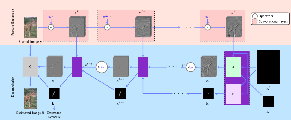
Fig. 1: Structure of the deep network constructed by algorithm unrolling and cascaded filtering. Block $A$ and $B$ implements Step 5 and Step 8 in Algorithm 1 respectively, while block $C$ implements (4). A diagram representation can be found at http://signal.ee.psu.edu/diagram.pdf. Intermediate data (hidden layers) on the trained network are also shown. It can be observed that, as $l$ increases, more details are extracted in ${\bf g}^{l}$ and finer kernel coefficients are recovered. The parameters that will be learned from real datasets are colored in blue.

2.2 Network Construction via Algorithm Unrolling

Each step of Algorithm 1 is in analytic form and can be implemented using a series of basic functional operations. Therefore, each iteration of Algorithm 1 admits a layered representation, and repeating it $L$ times yields an $L$-layer neural network (assuming $L$ iterations). For notational brevity, we concatenate the parameters in each layer and let $\mathbf{f}^{l}={(\mathbf{f}_{i}^{l})}_{i=1}^{C},\zeta^{l}={(\zeta_{i}^{l})}_{i=1}^{C},\lambda^{l}={(\lambda_{i}^{l})}_{i=1}^{C}$ and $\eta={(\eta_{i})}_{i=1}^{C}$. We also concatenate ${\bf y}_{i}^{l}$’s, ${\bf z}_{i}^{l}$’s and ${\bf g}_{i}^{l}$’s by letting ${\bf y}^{l}={({\bf y}_{i}^{l})}_{i=1}^{C}$, ${\bf z}^{l}={({\bf z}_{i}^{l})}_{i=1}^{C}$ and ${\bf g}^{l}={({\bf g}_{i}^{l})}_{i=1}^{C}$, respectively.

To handle large blur kernels, we alter the size of the filter banks ${\{\mathbf{f}_{i}\}}_{i}$ in different layers in the following way:

$$\text{size of }\mathbf{f}_{i}^{1}>\text{ size of }\mathbf{f}_{i}^{2}>\text{ size of }\mathbf{f}_{i}^{3}>\dots.$$

so that high-level representations features are captured first, and fine details emerge in later iterations. To facilitate training, we produce large filters by cascading small $3\times 3$ filters, following the same principle as [25]. Formally speaking, we set $\mathbf{f}_{i}^{L}={\bf w}_{i1}^{L}$ where ${\{{\bf w}_{i1}^{L}\}}_{i=1}^{C}$ is a collection of $3\times 3$ filters, and recursively obtain $\mathbf{f}_{i}^{l}$ by: $\mathbf{f}_{i}^{l}\leftarrow\sum_{j=1}^{C}{\bf w}_{ij}^{l}\ast\mathbf{f}_{j}^{l+1}.$ Using this representation, we obtain the network structure in Fig. 1. The parameters ${\{{\bf w}^{l},b^{l},\lambda^{l}\}}_{l=1}^{L}$ will be learned from the training data, as explained in the next Section.

(a) Groundtruth

(b) Perrone et al. [23]

(c) Nah et al. [26]

(d) DAU

Fig. 2: Qualitative comparisons on the BSDS500 dataset [27]. The blur kernels are placed at the right below corner. DAU recovers the kernel at higher accuracy and therefore the estimated images are more faithful to the groundtruth.

(a) Groundtruth

(b) Perrone et al. [23]

(c) Nah et al. [26]

(d) Chakrabarti [19]

(e) Xu et al. [20]

(f) DAU

Fig. 3: Qualitative comparisons on the dataset from [28]. The blur kernels are placed at the right below corner. DAU generates fewer artifacts and preserves more details than competing state of the art methods.

3 Experiments

Table 1: Quantitative comparison averaged over 200 images from the BSDS500 [27] set and 4 linear kernels. The RMSE values are computed over kernels. Best scores are in bold.

Metrics	DAU	[23]	[26]
PSNR (dB)	$\mathbf{27.21}$	$22.23$	$25.23$
ISNR (dB)	$\mathbf{4.36}$	$2.06$	$1.88$
SSIM	$\mathbf{0.88}$	$0.76$	$0.81$
RMSE ($\times 10^{-3}$)	$\mathbf{2.21}$	$5.21$	$-$

Table 2: Quantitative comparison on nonlinear motion (average over 4 images and 8 kernels from [28]). The RMSE values are computed over kernels. Best scores are in bold.

	DAU	[23]	[26]	[19]	[20]
PSNR (dB)	$\mathbf{27.15}$	$26.79$	$24.51$	$23.18$	$26.75$
ISNR (dB)	$\mathbf{3.79}$	$3.63$	$1.35$	$0.02$	$3.59$
SSIM	$0.88$	$\mathbf{0.89}$	$0.81$	$0.81$	$\mathbf{0.89}$
RMSE ($\times 10^{-3}$)	$3.87$	$\mathbf{3.83}$	$-$	$-$	$3.98$

Training: We use the training and validation portions from the Berkeley Segmentation Dataset (BSDS500) [27] as training images. The linear motion kernels are generated by uniformly sampling $16$ angles in $[0,\pi]$ and $16$ lengths in $[5,20]$. The images are convolved with each kernel and white Gaussian noise with standard deviation $0.01$ (suppose the image intensity is in $[0,1]$) is added. For each blurred image ${\bf y}_{t}^{\mathrm{train}}(t=1,\dots,T)$, we let the corresponding sharp image and kernel be ${\bf x}_{t}^{\mathrm{train}}$ and ${\bf k}_{t}^{\mathrm{train}}$, respectively. We re-parametrize $\lambda_{i}^{l}$ in step 6 of Algorithm 1 by letting $b_{i}^{l}=\lambda_{i}^{l}\zeta_{i}^{l}$ and let $b^{l}={(b_{i}^{l})}_{i=1}^{C},l=1,\dots,L$. The network outputs $\widetilde{{\bf x}}_{t},\widetilde{{\bf k}}_{t}$ corresponding to ${\bf y}^{\mathrm{train}}_{t}$ depend on the network parameters ${\bf w}^{l}$, $b^{l},\lambda^{l}$, $l=1,2,\dots,L$, and $\widetilde{{\bf x}}_{t}$ further depends on $\eta$. We train the network to determine those parameters by minimizing:

$$\min_{{\{{\bf w}^{l},b^{l},\lambda^{l}\}}_{l=1}^{L},\eta} \sum_{t=1}^{T}\operatorname*{MSE}\left({\bf x}_{t}^{\mathrm{train}}-\widetilde{{\bf x}}_{t}\left({\{{\bf w}^{l},b^{l},\lambda^{l}\}}_{l=1}^{L},\eta\right)\right)$$

$$+ \kappa\operatorname*{MSE}\left({\bf k}_{t}^{\mathrm{train}}-\widetilde{{\bf k}}_{t}\left({\left\{{\bf w}^{l},b^{l},\lambda^{l}\right\}}_{l=1}^{L}\right)\right),$$

subject to $$b_{i}^{l}\geq 0,\,\lambda_{i}^{l}\geq 0,\quad l=1,\dots,L,i=1,\dots,C,$$

where $\kappa>0$ is a constant parameter which is fixed to $10^{5}$ and $\operatorname*{MSE}$ is the Mean Squared Error. We choose $L=10$ and $C=16$ by cross-validation. The minimization is performed by stochastic gradient descent, followed by a gradient projection step to enforce the non-negative constraints. We use the Adam [29] solver for faster training. The learning rate is set to $1\times 10^{-3}$ initially and decayed by a factor of $0.9$ per epoch. We terminate training after $20$ epochs. The parameters ${\{\lambda_{i}^{l}\}}_{i,l}$ are initialized to zeros, ${\{b_{i}^{l}\}}_{i,l}$ to $1$, and ${\{\eta_{i}\}}_{i}$ to $20$, respectively. The weights are initialized according to [30].

Evaluation: We use $200$ images from the test portion from the BSDS500 dataset [27] as test images. We randomly choose angles from $[0,\pi]$ and lengths from $[5,20]$ to generate $4$ test kernels. We compare with state-of-the art algorithms, Perrone et al. [23] and Nah et al. [26], which are representatives of iterative algorithms and deep-learning approaches. We assess the performance using four commonly used evaluation metrics: Peak Signal-to-Noise-Ratio (PSNR), Improvement in Signal-to-Noise-Ratio (ISNR), Structural Similarity Index (SSIM) [31], and Root-Mean-Square Error (RMSE) between the estimated kernel and the groundtruth kernel. The average scores are in Table 1. Clearly, DAU outperforms state-of-the art algorithms by a significant margin.

Fig. 2 shows example images and kernels for a qualitative comparison. Although Perrone et al.’s method can roughly infer the directions of the blur kernels, the recovered coefficients are unsatisfactory. As a result, the recovered image contains clearly visible artifacts. Nah et al.’s method effectively removes most of the blurs, but blurring artifacts still remain locally and the details are not faithfully preserved. In contrast, the kernel recovered by DAU is closer to the ground truth and hence leads to a more accurate estimated image.

Additionally, we compare the performance of various methods on deblurring under non-linear motion kernels, which is a more realistic scenario as discussed in [28]. We collect training kernels by interpolating the paths provided by [32] and created by ourselves in the same manner. We further augment these kernels by scaling and rotations. We use the standard image set from [28] (comprising 4 images and 8 kernels) as the test set. The average scores are presented in Table 2. Again DAU outperforms state-of-the-art methods. A visual example is shown in Fig. 3,

4 Conclusion

We propose a neural network deblurring architecture built by unrolling an iterative algorithm. We show how a generalized TV-regularized algorithm can be recast into a neural network, and train it to optimize the parameters. Unlike most existing deblurring networks, our work has the benefit of interpretability, while exhibiting performance benefits that are shared with modern deep-nets and exceed state of the art performance.

References

- [1] D. Kundur and D. Hatzinakos, “Blind image deconvolution,” IEEE Signal Process. Mag., vol. 13, no. 3, pp. 43–64, May 1996.
- [2] N. Joshi, R. Szeliski, and D. J. Kriegman, “PSF estimation using sharp edge prediction,” in Proc. IEEE Conf. CVPR, June 2008.
- [3] Qi Shan, Jiaya Jia, and Aseem Agarwala, “High-quality Motion Deblurring from a Single Image,” in Proc. ACM SIGGRAPH, 2008.
- [4] Sunghyun Cho and Seungyong Lee, “Fast Motion Deblurring,” in Proc. ACM SIGGRAPH Asia, 2009.
- [5] Li Xu and Jiaya Jia, “Two-phase kernel estimation for robust motion deblurring,” in Proc. ECCV, 2010.
- [6] Dilip Krishnan, Terence Tay, and Rob Fergus, “Blind deconvolution using a normalized sparsity measure,” in Proc. IEEE Conf. CVPR, 2011.
- [7] L. Xu, S. Zheng, and J. Jia, “Unnatural L0 Sparse Representation for Natural Image Deblurring,” in Proc. IEEE Conf. CVPR, June 2013.
- [8] L. Sun, S. Cho, J. Wang, and J. Hays, “Edge-based blur kernel estimation using patch priors,” in Proc. IEEE ICCP, Apr. 2013.
- [9] J. Pan, Z. Hu, Z. Su, and M. H. Yang, “$L_0$ -Regularized Intensity and Gradient Prior for Deblurring Text Images and Beyond,” IEEE Trans. Pattern Anal. Mach. Intell., vol. 39, no. 2, pp. 342–355, Feb. 2017.
- [10] Jian-Feng Cai, Hui Ji, Chaoqiang Liu, and Zuowei Shen, “Framelet-Based Blind Motion Deblurring From a Single Image,” IEEE Trans. Image Process., vol. 21, no. 2, pp. 562–572, Feb. 2012.
- [11] Shiming Xiang, Gaofeng Meng, Ying Wang, Chunhong Pan, and Changshui Zhang, “Image Deblurring with Coupled Dictionary Learning,” Int. J. Comput. Vis., vol. 114, no. 2-3, pp. 248–271, Sept. 2015.
- [12] J. Pan, D. Sun, H. Pfister, and M. H. Yang, “Deblurring Images via Dark Channel Prior,” IEEE Trans. Pattern Anal. Mach. Intell., vol. PP, no. 99, pp. 1–1, 2018.
- [13] M. Tofighi, Y. Li, and V. Monga, “Blind image deblurring using row–column sparse representations,” IEEE Signal Processing Letters, vol. 25, no. 2, pp. 273–277, 2018.
- [14] Rob Fergus, Barun Singh, Aaron Hertzmann, Sam T. Roweis, and William T. Freeman, “Removing Camera Shake from a Single Photograph,” in Proc. ACM SIGGRAPH, New York, NY, USA, 2006.
- [15] A. Levin, Y. Weiss, F. Durand, and W. T. Freeman, “Efficient marginal likelihood optimization in blind deconvolution,” in Proc. IEEE Conf. CVPR, June 2011.
- [16] S. Derin Babacan, Rafael Molina, Minh N. Do, and Aggelos K. Katsaggelos, “Bayesian Blind Deconvolution with General Sparse Image Priors,” in Proc. ECCV, Oct. 2012.
- [17] Li Xu, Jimmy SJ Ren, Ce Liu, and Jiaya Jia, “Deep convolutional neural network for image deconvolution,” in Proc. NIPS, 2014.
- [18] R. Yan and L. Shao, “Blind Image Blur Estimation via Deep Learning,” IEEE Trans. Image Process., vol. 25, no. 4, pp. 1910–1921, Apr. 2016.
- [19] Ayan Chakrabarti, “A Neural Approach to Blind Motion Deblurring,” in Proc. ECCV, Oct. 2016.
- [20] X. Xu, J. Pan, Y. J. Zhang, and M. H. Yang, “Motion Blur Kernel Estimation via Deep Learning,” IEEE Trans. Image Process., vol. 27, no. 1, pp. 194–205, Jan. 2018.
- [21] Karol Gregor and Yann LeCun, “Learning fast approximations of sparse coding,” in Proc. ICML, 2010.
- [22] Christian J. Schuler, Michael Hirsch, Stefan Harmeling, and Bernhard Scholkopf, “Learning to Deblur,” IEEE Trans. Pattern Anal. Mach. Intell., vol. 38, no. 7, pp. 1439–1451, July 2016.
- [23] Daniele Perrone and Paolo Favaro, “A Clearer Picture of Total Variation Blind Deconvolution,” IEEE Trans. Pattern Anal. Mach. Intell., vol. 38, no. 6, pp. 1041–1055, June 2016.
- [24] Y. Wang, J. Yang, W. Yin, and Y. Zhang, “A New Alternating Minimization Algorithm for Total Variation Image Reconstruction,” SIAM J. Imaging Sci., vol. 1, no. 3, pp. 248–272, Jan. 2008.
- [25] Karen Simonyan and Andrew Zisserman, “Very deep convolutional networks for large-scale image recognition,” in Proc. ICLR, 2015.
- [26] Seungjun Nah, Tae Hyun Kim, and Kyoung Mu Lee, “Deep multi-scale convolutional neural network for dynamic scene deblurring,” in Proc. IEEE Conf. CVPR, 2017, vol. 1, p. 3.
- [27] D. Martin, C. Fowlkes, D. Tal, and J. Malik, “A database of human segmented natural images and its application to evaluating segmentation algorithms and measuring ecological statistics,” in Proc. IEEE ICCV, July 2001.
- [28] Anat Levin, Yair Weiss, Fredo Durand, and William T. Freeman, “Understanding and evaluating blind deconvolution algorithms,” in Computer Vision and Pattern Recognition, 2009. CVPR 2009. IEEE Conference on. 2009, pp. 1964–1971, IEEE.
- [29] Diederik P. Kingma and Jimmy Ba, “Adam: A method for stochastic optimization,” in Proc. ICLR, 2015.
- [30] Xavier Glorot and Yoshua Bengio, “Understanding the difficulty of training deep feedforward neural networks,” in Proc. ICAIS, Mar. 2010.
- [31] Zhou Wang, A.C. Bovik, H.R. Sheikh, and E.P. Simoncelli, “Image quality assessment: from error visibility to structural similarity,” IEEE Trans. Image Process., vol. 13, no. 4, pp. 600–612, Apr. 2004.
- [32] Rolf Köhler, Michael Hirsch, Betty Mohler, Bernhard Schölkopf, and Stefan Harmeling, “Recording and playback of camera shake: Benchmarking blind deconvolution with a real-world database,” in European Conference on Computer Vision. 2012, pp. 27–40, Springer.