Cross-correlated shot noise in three-terminal superconducting hybrid nanostructures

Abstract

We work out a unified theory describing both non-local electron transport and cross-correlated shot noise in a three-terminal normal-superconducting-normal (NSN) hybrid nanostructure. We describe noise cross correlations both for subgap and overgap bias voltages and for arbitrary distribution of channel transmissions in NS contacts. We specifically address a physically important situation of diffusive contacts and demonstrate a non-trivial behavior of non-local shot noise exhibiting both positive and negative cross correlations depending on the bias voltages. For this case, we derive a relatively simple analytical expression for cross-correlated noise power which contains only experimentally accessible parameters.

I Introduction

It is well known that a normal metal attached to a superconductor also acquires superconducting properties. At low enough temperatures proximity induced superconducting correlations may spread at long distances inside the normal metal leading to a wealth of interesting phenomena Bel . Furthermore, electrons in two different normal metals may become coherent provided these metals are connected through a superconducting island with effective thickness $d$ shorter than the superconducting coherence length $\xi$. This effect has to do with the phenomenon of the so-called crossed Andreev reflection (CAR), in which a Cooper pair may split into two electrons going in two different normal leads DF , see Fig. 1d. This Cooper pair splitting process may be used to generate pairs of entangled electrons in different metallic electrodes Lesovik ; Buttiker ; Brange , i.e. to experimentally realize a quantum phenomenon that could be of crucial importance for developing quantum communication technologies.

Crossed Andreev reflection is a quantum coherent process, which strongly affects electron transport in three-terminal normal metal - superconductor - normal metal (NSN) hybrid structures at sufficiently low temperatures. This issue triggered a substantial theoretical FFH ; BG ; KZ1 ; KZ2 ; Belzig ; GZ07 ; LY ; GKZ (see also further references therein) and experimental Beck1 ; Teun ; Venkat1 ; Hof ; Saclay ; Basel3 ; Basel ; Beck2 ; Beck3 interest over past years and is presently quite well understood.

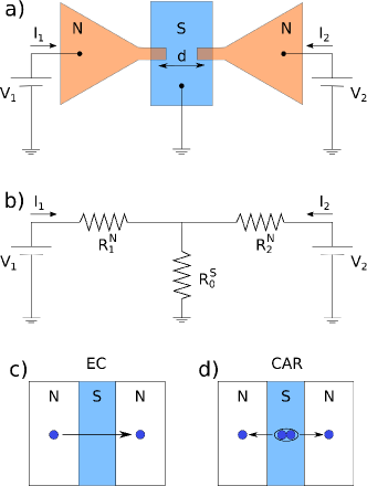
Figure 1: (a) Schematics of an NSN structure under consideration. The contacts between the normal leads and the superconductor (located at a distance $d$ from each other) may be described by an arbitrary distribution of channel transmissions or, else, may have a shape of short diffusive wires. (b) Equivalent circuit of the same system in the normal state. Here $R_{1}^{N}$ and $R_{2}^{N}$ are the junction resistances and $R_{0}^{S}$ is the normal state resistance of the superconducting lead. (c) Schematics of elastic cotunneling (EC) process in which an electron is transferred from one normal terminal to another one through an effective barrier formed by a superconductor. (d) Schematics of crossed Andreev reflection (CAR) process corresponding to splitting of a Cooper pair into two entangled electrons located in two normal terminals.

Consider, e.g., an NSN structure depicted in Fig. 1a. Applying bias voltages $V_{1}$ ad $V_{2}$ to two normal metallic electrodes and measuring electric currents $I_{1}$ and $I_{2}$ (depending on both voltages $V_{1}$ ad $V_{2}$) it becomes possible to identify the contribution of CAR to non-local electron transport in such a structure. In fact, CAR is not the only process which contributes to the non-local transport in this case. It competes with the so-called elastic cotunneling (EC), which does not produce entangled electrons. In the course of the latter process an electron is being transferred from one normal metal to another overcoming the effective barrier created by the energy gap inside the superconductor (see Fig. 1c). In the zero temperature limit EC and CAR contributions to the low bias non-local conductance $\partial I_{1}/\partial V_{2}$ cancel each other in NSN structures with low transparency contactsFFH .

One possible way to discriminate between CAR and EC processes is to investigate fluctuations of the currents $I_{1}$ and $I_{2}$. It is well known that in normal (i.e. non-superconducting) multiterminal structures cross correlations of current noise in different terminals are always negative due to the Pauli exclusion principle for electrons BB . In the presence of superconductivity such cross correlations may become positive due to CAR. Hence, by measuring cross-correlated current noise in a system like the one depicted in Fig. 1a it is possible to provide a clear experimental evidence for the presence of CAR in the system.

A theoretical treatment of cross-correlated non-local current noise in NSN structures was pioneered in the works Belzig3 ; Hekking for the case of tunnel barriers at NS interfaces, and in the work Samuelsson for a chaotic cavity coupled to normal and superconducting electrodes. This treatment indeed demonstrated that at certain voltage bias values CAR can dominate non-local shot noise giving rise to positive cross correlations. Later on theoretical analysis of noise cross correlations was extended to the case of arbitrary barrier transmissions Melin2 ; Belzig2 ; GZ ; Melin ; Melin3 ; Ostrove . In particular, for fully open barriers and at low enough temperature positive cross correlations were predicted to occur at any non-zero voltage bias values GZ . Positively cross-correlated non-local shot noise was also observed in several experiments Ch ; Das .

In this work we extend the existing theory of non-local shot noise in NSN hybridsGZ , developed for non-interacting electrons, in at least two important aspects. Firstly, here we relax the assumption GZ restricting the energy to subgap values and develop the analysis of both non-local electron transport and non-local shot noise at any voltage bias values $V_{1,2}$ and temperature $T$ both below and above the superconducting gap $\Delta$. Secondly, we do not anymore assume (unlike it was done in GZ ) that transmission probabilities for all conducting channels in the junction are equal and allow for an arbitrary transmission distribution. Following the analysis GZ , we perform the lowest order expansion in the small ratio between the normal state resistance of the superconducting lead $R_{0}^{S}$ and the interface resistances $R_{1,2}^{N}$ (see Fig. 1b), which allows us to perform disorder averaging in a superconducting terminal exactly. In this way, we derive a general analytical expression for the cross-correlated non-local noise in the two contacts (86). We specifically address an important case of diffusive contacts, where the expression for the noise (83) greatly simplifies and contains only experimentally accessible parameters.

The structure of the paper is as follows. In Sec. II we derive a general expression for the cumulant generating function in an NSN structure with arbitrary distribution of conducting channel transmissions. In Sec. III we briefly recollect the results for both local electron transport and local shot noise in a single NS contact thereby preparing our subsequent consideration of non-local effects. Non-local transport and non-local shot noise are addressed in details in Sec. IV paying special attention to an important physical situation of diffusive NS junctions. A couple of general and rather lengthy results are relegated to Appendix.

II Cumulant generating function

In what follows we will consider an NSN structure depicted in Fig. 1a. Normal metallic leads are connected to a bulk superconductor by two junctions characterized by a set of transmission probabilities $\tau_{1,n}$ and $\tau_{2,n}$, where $n$ is the integer number enumerating all conducting channels. The two junctions are located at a distance $d$ from each other which is assumed to be shorter that the superconducting coherence length $\xi$.

Let $P_{t}(N_{1},N_{2})$ be the probability for $N_{1}$ and $N_{2}$ electrons to be transferred respectively through the junctions 1 and 2 during the observation time $t$. It is instructive to introduce the so-called cumulant generating function (CGF) ${\cal F}(\chi_{1},\chi_{2})$ by means of the relation

$$e^{{\cal F}(\chi_{1},\chi_{2})}=\sum_{N_{1},N_{2}}e^{-iN_{1}\chi_{1}-iN_{2}\chi_{2}}P_{t}(N_{1},N_{2}).$$ (1)

The parameters $\chi_{1}$ and $\chi_{2}$ are denoted as counting fields. The average currents through the junctions $I_{r}=\langle\hat{I}_{r}(t)\rangle$, and the correlation functions of the currents,

$$S_{rr^{\prime}} = \frac{1}{2}\int dt\big{[}\big{\langle}\hat{I}_{r}(t_{0}+t)\hat{I}_{r^{\prime}}(t_{0})+\hat{I}_{r^{\prime}}(t_{0})\hat{I}_{r}(t_{0}+t)\big{\rangle}$$ (2)

$$-\,2\langle I_{r}(t_{0})\big{\rangle}\langle I_{r^{\prime}}(t_{0})\big{\rangle}\big{]}$$

are expressed via the CGF as follows

$$I_{r} = \lim_{t\to 0}\frac{ie}{t}\frac{\partial{\cal F}}{\partial\chi_{r}}\bigg{|}_{\chi_{r}=0},$$

$$S_{rr^{\prime}} = -\lim_{t\to 0}\frac{e^{2}}{t}\frac{\partial^{2}{\cal F}}{\partial\chi_{r}\partial\chi_{r^{\prime}}}\bigg{|}_{\chi_{r}=0}.$$ (3)

In order to evaluate the CGF for the system depicted in Fig. 1 we will make use of the effective action approach GZ . The Hamiltonian of our system is expressed in the form

$$H=H_{1}+H_{2}+H_{S}+H_{T,1}+H_{T,2},$$ (4)

where $H_{1,2}$ are the Hamiltonians of the normal leads,

$$H_{r}=\sum_{\alpha=\uparrow,\downarrow}\int d{\bm{x}}\ \hat{\psi}^{\dagger}_{r,\alpha}({\bm{x}})\left(-\frac{\nabla^{2}}{2m}-\mu-eV_{r}\right)\hat{\psi}_{r,\alpha}({\bm{x}}),$$ (5)

$\hat{\psi}^{\dagger}_{r,\alpha}({\bm{x}}),\hat{\psi}_{r,\alpha}({\bm{x}})$ are the creation and annihilation operators for an electron with a spin projection $\alpha$ at a point ${\bm{x}}$, $m$ is the electron mass, $\mu$ is the chemical potential, $V_{r}$ is the electric potential applied to the lead $r$,

$$H_{S} = \int d{\bm{x}}\bigg{[}\sum_{\alpha}\hat{\psi}^{\dagger}_{S,\alpha}({\bm{x}})\left(-\frac{\nabla^{2}}{2m}-\mu+U_{\rm dis}({\bm{x}})\right)\hat{\psi}_{S,\alpha}({\bm{x}})$$ (6)

$$+\,\Delta\hat{\psi}^{\dagger}_{S,\uparrow}({\bm{x}})\hat{\psi}^{\dagger}_{S,\downarrow}({\bm{x}})+\Delta^{*}\hat{\psi}_{S,\downarrow}({\bm{x}})\hat{\psi}_{S,\uparrow}({\bm{x}})\bigg{]}$$

is the Hamiltonian of a superconducting electrode with the order parameter $\Delta$ and disorder potential $U_{\rm dis}({\bm{x}})$, and the terms

$$H_{T,r} = \int_{{\cal A}_{r}}d^{2}{\bm{x}}\sum_{\alpha=\uparrow,\downarrow}\big{[}t_{r}({\bm{x}})\hat{\psi}^{\dagger}_{r,\alpha}({\bm{x}})\hat{\psi}_{S,\alpha}({\bm{x}})$$ (7)

$$+\,t_{r}^{*}({\bm{x}})\hat{\psi}_{S,\alpha}^{\dagger}({\bm{x}})\hat{\psi}_{r,\alpha}({\bm{x}})\big{]}$$

describe electron transfer through the contacts between the superconductor and the normal leads. In Eq. (7) the surface integrals run over the contact areas ${\cal A}_{r}$, and $t_{r}({\bm{x}})$ are the coordinate dependent tunneling amplitudes. Note that here we do not consider the case of spin active interfaces KZ2 , hence the amplitudes $t_{r}({\bm{x}})$ do not depend on the spin projection.

One can introduce the wave functions in the leads corresponding to incoming and outgoing scattering states in the $n-$th conducting channel of the $r-$th junction, $\psi_{r,n}({\bm{x}})$, and expand the electronic operators as

$$\hat{\psi}_{r,\alpha}({\bm{x}}) = \sum_{n}\psi_{r,n}({\bm{x}})\hat{a}_{n,\alpha},$$

$$\hat{\psi}_{S,\alpha}({\bm{x}}) = \sum_{n}\psi_{S,n}({\bm{x}})\hat{c}_{n,\alpha}.$$ (8)

The Hamiltonians (7) then acquire the form

$$H_{T,r}=\sum_{\alpha=\uparrow,\downarrow}\sum_{n}[t_{r,n}\hat{a}^{\dagger}_{n,\alpha}\hat{c}_{n,\alpha}+t_{r,n}^{*}\hat{c}^{\dagger}_{n,\alpha}\hat{a}_{n,\alpha}],$$ (9)

where $t_{r,n}=\int_{{\cal A}_{r}}d^{2}{\bm{x}}\psi_{S,n}^{*}({\bm{x}})t_{r}({\bm{x}})\psi_{r,n}({\bm{x}})$ are the matrix elements of the tunneling amplitude. These matrix elements are related to the channel transmission probabilities $\tau_{r,n}$ by means of the standard relation Carlos

$$\tau_{r,n}={4\alpha_{r,n}}/{(1+\alpha_{r,n})^{2}},$$ (10)

with $\alpha_{r,n}=\pi^{2}\nu_{r}\nu_{S}|t_{r,n}|^{2}$ and $\nu_{j}$ being the density of states in the corresponding electrode (here $j=1,2,S$).

The CGF (1) can formally be expressed as

$${\cal F}=\ln\left[{\rm tr}\left(e^{-i\chi_{1}\hat{N}_{1}-i\chi_{2}\hat{N}_{2}}e^{-iHt}e^{i\chi_{1}\hat{N}_{1}+i\chi_{2}\hat{N}_{2}}\hat{\rho}_{0}e^{iHt}\right)\right],$$

(11)

where $\hat{N}_{r}=\sum_{\alpha=\uparrow,\downarrow}\sum_{n}\hat{a}_{\alpha,n}^{\dagger}\hat{a}_{\alpha,n}$ are the electron number operators in the normal leads and $\hat{\rho}_{0}=\exp(-H/T)/{\rm tr}[\exp(-H/T)]$ is the equilibrium density matrix of the system. The above expression can identically be transformed to

$${\cal F}=\ln\left[{\rm tr}\left(e^{-iH(\chi_{1},\chi_{2})t}\hat{\rho}_{0}e^{iH(-\chi_{1},-\chi_{2})t}\right)\right],$$ (12)

where

$$H(\chi_{1},\chi_{2})=e^{-i(\chi_{1}\hat{N}_{1}+\chi_{2}\hat{N}_{2})/2}He^{i(\chi_{1}\hat{N}_{1}+\chi_{2}\hat{N}_{2})/2}$$

$$=\,H_{1}+H_{2}+H_{S}+H_{T,1}(\chi_{1})+H_{T,2}(\chi_{2})$$ (13)

and

$$H_{T,r}(\chi)=e^{-i\chi_{r}\hat{N}_{r}/2}H_{T,r}e^{i\chi_{r}\hat{N}_{r}/2}$$

$$=\,\sum_{\alpha=\uparrow,\downarrow}\sum_{n}[t_{r,n}e^{i\chi_{r}/2}\hat{c}^{\dagger}_{n,\alpha}\hat{a}_{n,\alpha}+t_{r,n}^{*}e^{-i\chi_{r}/2}\hat{a}^{\dagger}_{n,\alpha}\hat{c}_{n,\alpha}].$$

The CGF (12) can be evaluated in a straightforward manner with the aid of the path integral technique GZ which yields

$${\cal F}(\chi_{1},\chi_{2})={\rm tr}\,[\ln\hat{\cal G}^{-1}(\chi_{1},\chi_{2})],$$ (14)

where $\hat{\cal G}^{-1}$ is the Keldysh Green function of our system

$${\cal G}^{-1}(\chi_{1},\chi_{2})=\left(\begin{array}[]{ccc}\check{G}_{1}^{-1}&\check{t}_{1}(\chi_{1})&0\\ \check{t}_{1}^{\dagger}(\chi_{1})&\check{G}_{S}^{-1}&\check{t}_{2}(\chi_{2})\\ 0&\check{t}_{2}^{\dagger}(\chi_{2})&\check{G}_{2}^{-1}\end{array}\right),$$ (18)

the $4\times 4$ matrices $\check{G}_{j}^{-1}$ represent the inverse Keldysh Green functions of isolated normal and superconducting leads and $\check{t}_{r}$ is the diagonal $4\times 4$ matrix in the Nambu - Keldysh space describing tunneling between the leads,

$$\check{t}_{r}(\chi_{r})=\left(\begin{array}[]{cccc}-t_{r}e^{-i\frac{\chi_{r}}{2}}&0&0&0\\ 0&t_{r}e^{i\frac{\chi_{r}}{2}}&0&0\\ 0&0&t_{r}e^{i\frac{\chi_{r}}{2}}&0\\ 0&0&0&-t_{r}e^{-i\frac{\chi_{r}}{2}}\end{array}\right).$$ (23)

The CGF (14) can be cast to the form

$${\cal F}={\rm tr}\ln\big{[}\check{I}-\check{t}_{1}^{\dagger}\check{G}_{1}\check{t}_{1}\check{G}_{S}-\check{t}_{2}^{\dagger}\check{G}_{2}\check{t}_{2}\check{G}_{S}\big{]}.$$ (24)

where $\check{I}$ is the unity operator.

The Fourier transformed Green function of a superconducting island, $\check{G}_{S}(E)=\int dt\,e^{iE(t-t^{\prime})}\check{G}_{S}(t-t^{\prime},{\bm{x}},{\bm{x}}^{\prime})$, reads

$$\check{G}_{S}(E) = \frac{\hat{G}_{R}(E)+\hat{G}_{A}(E)}{2}\otimes\hat{\sigma}_{z}$$ (25)

$$+\,\frac{\hat{G}_{R}(E)-\hat{G}_{A}(E)}{2}\otimes\hat{Q}_{S}(E)\hat{\sigma}_{z}.$$

Here

$$\hat{G}_{R,A}(E)=\left(\begin{array}[]{cc}G_{R,A}(E,{\bm{x}},{\bm{x}}^{\prime})&F^{+}_{R,A}(E,{\bm{x}},{\bm{x}}^{\prime})\\ F_{R,A}(E,{\bm{x}},{\bm{x}}^{\prime})&G^{+}_{R,A}(E,{\bm{x}},{\bm{x}}^{\prime})\end{array}\right)$$ (31)

$$=\,\sum_{n}\frac{\varphi_{n}({\bm{x}})\varphi_{n}^{*}({\bm{x}}^{\prime})}{(E\pm i0)^{2}-\xi_{n}^{2}-|\Delta|^{2}}\left(\begin{array}[]{cc}E+\xi_{n}&\Delta^{*}\\ \Delta&E-\xi_{n}\end{array}\right),$$

(32)

are retarded and advanced Green functions and the matrix

$$\hat{Q}_{S}(E)=\left(\begin{array}[]{cc}1-2n_{S}(E)&2n_{S}(E)\\ 2-2n_{S}(E)&2n_{S}(E)-1\end{array}\right)$$ (35)

depends on the quasiparticle distribution function $n_{S}(E)$ in a superconductor and has the property $\hat{Q}^{2}(E)=1$. The wave functions $\varphi_{n}({\bm{x}})$, appearing in Eq. (32) are the eigenfunctions of a single electron Hamiltonian of the superconducting lead with eigenenergies $\xi_{n}$, i.e. they are the solutions of the Schrödinger equation

$$\left(-\frac{\nabla^{2}}{2m}-\mu+U_{\rm dis}({\bm{x}})\right)\varphi_{n}({\bm{x}})=\xi_{n}\varphi_{n}({\bm{x}}).$$ (36)

Note that the wave functions $\varphi_{n}({\bm{x}})$ differ from the functions $\psi_{r,n}({\bm{x}})$ introduced earlier in Eqs. (8). The expressions for the Green functions in the normal leads are recovered from Eqs. (25)-(35) by replacing $S\to r=1,2$ and setting $\Delta=0$.

Following the analysis GZ let us define the self-energies $\check{\Sigma}_{r}(\chi_{r})=\check{t}^{\dagger}_{r}\check{G}_{r}\check{t}_{r}$ and derive their matrix elements in the basis of the scattering states wave functions in the corresponding contact. We obtain

$$\check{\Sigma}_{r}^{mn}(\chi_{r},E)=\int_{{\cal A}_{r}}d^{2}{\bm{x}}d^{2}{\bm{x}}^{\prime}\,\psi_{S,m}^{*}({\bm{x}})\check{t}^{\dagger}_{r}(\chi_{r},{\bm{x}})$$

$$\times\,\check{G}_{r}(E,{\bm{x}},{\bm{x}}^{\prime})\check{t}_{r}(\chi_{r},{\bm{x}}^{\prime})\psi_{S,n}({\bm{x}}^{\prime})$$

$$=\,\frac{\alpha_{r,n}}{\pi i\nu_{S}}\delta_{mn}\left(\begin{array}[]{c}\hat{\sigma}_{z}e^{-i\frac{\hat{\sigma}_{z}\chi}{2}}\hat{Q}(E-eV_{r})e^{i\frac{\hat{\sigma}_{z}\chi}{2}}\qquad 0\\ 0\qquad\hat{\sigma}_{z}e^{i\frac{\hat{\sigma}_{z}\chi}{2}}\hat{Q}(E+eV_{r})e^{-i\frac{\hat{\sigma}_{z}\chi}{2}}\end{array}\right),$$ (39)

(40)

where the matrices $\hat{Q}_{r}(E)$ are defined in the same way as in Eq. (35), i.e.

$$\hat{Q}_{r}(E)=\left(\begin{array}[]{cc}1-2n_{r}(E)&2n_{r}(E)\\ 2-2n_{r}(E)&2n_{r}(E)-1\end{array}\right),$$ (43)

and $n_{r}(E)$ are the distribution functions of electrons in the normal leads. Note that by performing a proper rotation in the basis of the scattering wave functions in the superconductor one can always diagonalize the self-energies $\check{\Sigma}_{r}^{mn}\propto\delta_{mn}$. Hence, the CGF (24) can be expressed in the form

$${\cal F}(\chi_{1},\chi_{2})={\rm tr}\,\ln\big{[}\check{I}-\check{\Sigma}_{1}(\chi_{1})\check{G}_{S}-\check{\Sigma}_{2}(\chi_{2})\check{G}_{S}\big{]}.$$ (44)

Unfortunately, the CGF (44) cannot be evaluated exactly. In order to proceed and to account for the effects of CAR we carry out a perturbative expansion of the CGF (44) in powers of the ”off-diagonal” component of the superconductor Green function $\check{G}_{S}({\bm{x}},{\bm{x}}^{\prime})$, in which the points ${\bm{x}}$ and ${\bm{x}}^{\prime}$ belong to different junctions. This expansion is justified provided the normal state resistance of the superconducting lead $R_{0}^{S}$ remains small as compared to the contact resistances $R_{1}^{N},R_{2}^{N}$, and it is essentially equivalent to linearizing the Usadel equation. The latter simplification is routinely performed Volkov1 in order to fully analytically describe various non-trivial non-equilibrium effects in superconducting hybrid structures, such as, e.g., the sign inversion of the Josephson critical current in SNS-like junctions Morpurgo ; Volkov2 . To this end, we define the operator $\check{A}=\check{\Sigma}_{1}(\chi_{1})\check{G}_{S}+\check{\Sigma}_{2}(\chi_{2})\check{G}_{S}$ and formally rewrite the expression (44) in the form

$${\cal F}(\chi_{1},\chi_{2})={\rm tr}\,\ln\left[\left(\begin{array}[]{cc}\check{I}_{11}-\check{A}_{11}&-\check{A}_{12}\\ -\check{A}_{21}&\check{I}_{22}-\check{A}_{22}\end{array}\right)\right],$$ (47)

where the subscripts indicate the contact at which the coordinates ${\bm{x}}$ (first index) or ${\bm{x}}^{\prime}$ (second index) are located. Expanding in the small ”off-diagonal” components $\check{A}_{12},\check{A}_{21}$ to the lowest non-vanishing order, we arrive at the result

$${\cal F}(\chi_{1},\chi_{2})={\cal F}_{1}(\chi_{1})+{\cal F}_{2}(\chi_{2})+{\cal F}_{12}(\chi_{1},\chi_{2}),$$ (48)

where

$${\cal F}_{r}(\chi_{r})={\rm tr}\,\ln\big{[}\check{I}-\check{\Sigma}_{r}(\chi_{r})\check{G}_{S,rr}\big{]},\;\;r=1,2$$ (49)

are the local contributions and the term

$${\cal F}_{12}(\chi_{1},\chi_{2}) = -t\int\frac{dE}{2\pi}{\rm tr}\left[(\check{I}_{11}-\check{\Sigma}_{1}(\chi_{1})\check{G}_{S,11})^{-1}\check{A}_{12}\right.$$ (50)

$$\times\,\left.(\check{I}_{22}-\check{\Sigma}_{2}(\chi_{2})\check{G}_{S,22})^{-1}\check{A}_{21}\right]$$

accounts for non-local effects. Note that in Eq. (50) we replaced the double time integration by a single integral over energy which is appropriate in the long time limit.

The expressions (49) and (50) contain the Green functions of the superconductor $G_{R,A}$, which oscillate at the scale of the Fermi wavelength. One can simplify these expressions by averaging over disorder. Such averaging can be handled with the aid of the following relations Brouwer :

$$\sum_{n}\langle\varphi_{n}({\bm{x}})\varphi_{n}^{*}({\bm{x}}^{\prime})\rangle\delta(\xi-\xi_{n})=\nu_{S}w(|{\bm{x}}-{\bm{x}}^{\prime}|),$$ (51)

$$\sum_{mn}\langle\varphi_{n}({\bm{x}})\varphi_{n}^{*}({\bm{x}}^{\prime})\varphi_{m}({\bm{x}}^{\prime})\varphi_{m}^{*}({\bm{x}})\rangle\delta(\xi-\xi_{n})\delta(\xi^{\prime}-\xi_{m})$$

$$=\,\nu_{S}^{2}w^{2}(|{\bm{x}}-{\bm{x}}^{\prime}|)+\frac{\nu_{S}}{\pi}\,{\rm Re}\,D(\xi-\xi^{\prime},{\bm{x}},{\bm{x}}^{\prime})$$

$$+\,\frac{\nu_{S}}{\pi}w^{2}(|{\bm{x}}-{\bm{x}}^{\prime}|)\,{\rm Re}\,C\left(\xi-\xi^{\prime},\frac{{\bm{x}}+{\bm{x}}^{\prime}}{2},\frac{{\bm{x}}+{\bm{x}}^{\prime}}{2}\right).$$ (52)

Here $w(r)=e^{-r/2l_{e}}\sin(k_{F}r)/k_{F}r$, $l_{e}$ is the mean free path of electrons, and $D(\omega,{\bm{x}},{\bm{x}}^{\prime})$, $C(\omega,{\bm{x}},{\bm{x}}^{\prime})$ are, respectively, the diffuson and the Cooperon.

In what follows we will assume that the distance between the two junctions is shorter than the effective dephasing length for electrons, in which case the diffuson and the Cooperon coincide with each other, $D(\omega,{\bm{x}},{\bm{x}}^{\prime})=C(\omega,{\bm{x}},{\bm{x}}^{\prime})$, being determined by the fundamental solution of the diffusion equation

$$(-i\omega-D_{S}\nabla_{{\bm{x}}}^{2})D(\omega,{\bm{x}},{\bm{x}}^{\prime})=\delta({\bm{x}}-{\bm{x}}^{\prime}),$$ (53)

where $D_{S}=v_{F}l_{e}/3$ is the diffusion constant in the superconductor.

Let us for simplicity ignore the influence of the proximity effect on local transport properties of the contacts and replace the Green functions $\check{G}_{S,11}$ and $\check{G}_{S,22}$ appearing in Eqs. (49), (50) by their disorder averaged values $\langle\check{G}_{S,11}\rangle$ and $\langle\check{G}_{S,22}\rangle$. Averaging of pairwise products of the Green function components $\check{G}_{S,12}$ and $\check{G}_{S,21}$ (contained in the non-local terms $\check{A}_{12}$ and $\check{A}_{21}$ in Eq. (50)) is carried out with the aid of Eq. (52). Further simplifications occur if we recall that the distance between the contacts $d$ remains shorter than the superconducting coherence length $\xi=\sqrt{D_{S}/2\Delta}$. In this case one can set $\omega=0$ in the argument of the diffuson, i.e. we replace $D(\omega,{\bm{x}},{\bm{x}}^{\prime})\to D(0,{\bm{x}},{\bm{x}}^{\prime})$. Finally, we also assume complete randomization of the electron trajectories connecting the two contacts inside a disordered superconductor, meaning that an electron leaving the junction 1 via the conduction channel $n$ has the same probability to arrive at the contact 2 in any of its conduction channels. In this way we bring the CGF (50) to the form

$${\cal F}_{12} = t\frac{2e^{2}R_{0}^{S}}{\pi}\sum_{n,m}\int dE\,{\rm tr}\left\{\left(\check{I}_{11}-\check{\Sigma}_{1}(\chi_{1})\langle\check{G}_{S,11}\rangle\right)_{n}^{-1}\right.$$ (54)

$$\times\,\left.\alpha_{1,n}\check{Q}_{1}\left(\check{I}_{22}-\check{\Sigma}_{2}(\chi_{2})\langle\check{G}_{S,22}\rangle\right)_{m}^{-1}\alpha_{2,m}\check{Q}_{2}\right.$$

$$\left.-\,\left[1-\left(\check{I}_{11}-\check{\Sigma}_{1}(\chi_{1})\langle\check{G}_{S,11}\rangle\right)_{n}^{-1}\right]\right.$$

$$\times\,\left.\left[1-\left(\check{I}_{22}-\check{\Sigma}_{2}(\chi_{2})\langle\check{G}_{S,22}\rangle\right)_{m}^{-1}\right]\right\},$$

where the sum runs over all conducting channels of the contact 1 (index $n$) and of the contact 2 (index $m$),

$$\check{Q}_{r}(E)=\left(\begin{array}[]{cc}\hat{Q}_{r}(E-eV_{r})&0\\ 0&-\hat{Q}_{r}(E+eV_{r})\end{array}\right),$$ (57)

and $R_{0}^{S}$ is the characteristic resistance which sets the scale for non-local effects in our system. It is defined as

$$R_{0}^{S}=\frac{1}{2e^{2}\nu_{S}{\cal A}_{1}{\cal A}_{2}}\int_{{\cal A}_{1}}d^{2}{\bm{x}}_{1}\int_{{\cal A}_{2}}d^{2}{\bm{x}}_{2}\,D(0,{\bm{x}}_{1},{\bm{x}}_{2})$$ (58)

being approximately equal to the total resistance of the superconducting electrode measured in the normal state between the ground and the region to which the normal leads are attached, see Fig. 1b.

Equation (54) for the non-local part of CGF represents the main result of this section which will be directly employed in our subsequent analysis.

III Local transport and noise in a single NS junction

Before turning to non-local effects let us briefly recollect the well known results for both electron transport and noise in single NS junctions paying special attention to the case of a diffusive interface between the two metals. Following a seminal work by Blonder, Tinkham and Klapwijk BTK we define the probabilities for scattering processes in the junction for every conducting channel. Specifically, these are the probabilities of Andreev reflection, $A_{r,n}$, of normal reflection, $B_{r,n}$, of normal transmission, $C_{r,n}$, and of the transmission with the conversion of an electron into a hole, $D_{r,n}$, in the junction $r$. At subgap energies $|E|<\Delta$ we have BTK

$$A_{r,n}(E)=\frac{4\alpha_{r,n}^{2}\Delta^{2}}{(1+\alpha_{r,n}^{2})^{2}\Delta^{2}-(1-\alpha_{r,n}^{2})^{2}E^{2}},$$ (59)

$B_{r,n}=1-A_{r,n}$, $C_{r,n}=D_{r,n}=0$; while at $|E|>\Delta$ one getsBTK

$$A_{r,n}(E) = \frac{4\alpha_{r,n}^{2}\left(N_{S}^{2}(E)-1\right)}{\left(1+\alpha_{r,n}^{2}+2\alpha_{r,n}N_{S}(E)\right)^{2}},$$

$$B_{r,n}(E) = \frac{(1-\alpha_{r,n}^{2})^{2}}{\left(1+\alpha_{r,n}^{2}+2\alpha_{r,n}N_{S}(E)\right)^{2}},$$

$$C_{r,n}(E) = \frac{2\alpha_{r,n}(1+\alpha_{r,n})^{2}\left(N_{S}(E)+1\right)}{\left(1+\alpha_{r,n}^{2}+2\alpha_{r,n}N_{S}(E)\right)^{2}},$$

$$D_{r,n}(E) = \frac{2\alpha_{r,n}(1-\alpha_{r,n})^{2}\left(N_{S}(E)-1\right)}{\left(1+\alpha_{r,n}^{2}+2\alpha_{r,n}N_{S}(E)\right)^{2}},$$ (60)

where $N_{S}(E)=\theta(|E|-\Delta)|E|/\sqrt{E^{2}-\Delta^{2}}$ is the density of states in the superconductor, and $\theta(x)$ is the Heaviside step function.

The CGF of a single contact (49) can be evaluated exactly, it is presented in Appendix, see the Eq. (85). This result allows one to immediately reconstruct the well-known expression for the (local) current (II) in the $r$-th junction BTK

$$I_{r}=\frac{e}{2\pi}\sum_{n}\int dE\,g(E,\alpha_{r,n})(n_{r}^{-}-n_{r}^{+}).$$ (61)

Here $n_{j}^{-}$ and $n_{j}^{+}$ are the distribution functions for respectively electrons and holes in the normal leads,

$$n_{r}^{\pm}=\frac{1}{1+e^{(E\pm eV_{r})/T_{r}}},$$ (62)

and

$$g(E,\alpha_{r,n})=2A_{r,n}(E)+C_{r,n}(E)+D_{r,n}(E)$$ (63)

is the dimensionless spectral conductance in the $n-$th channel.

The expression for local current noise in the $r$-th junction, given by the derivative (3),

$$S_{rr}=\frac{1}{2}\int dt\left[\left\langle\hat{I}_{r}(t)\hat{I}_{r}(0)+\hat{I}_{r}(0)\hat{I}_{r}(t)\right\rangle-2\left\langle\hat{I}_{r}(0)\right\rangle\right],$$ (64)

is recovered analogously. We get MK ; AD

$$S_{rr}=\frac{e^{2}}{2\pi}\sum_{n}\int dE\bigg{[}4\,\theta(\Delta-|E|)\,A_{r,n}(1-A_{r,n})$$

$$\times\,w(n_{r}^{-},n_{r}^{+})+\left(C_{r,n}+D_{r,n}-(C_{r,n}-D_{r,n})^{2}\right)$$

$$\times\,(w(n_{r}^{-},n_{S})+w(n_{r}^{+},n_{S}))$$

$$+\,(2A_{r,n}+C_{r,n}+D_{r,n})^{2}\frac{w(n_{r}^{-},n_{r}^{-})+w(n_{r}^{+},n_{r}^{+})}{2}$$

$$+\,(C_{r,n}-D_{r,n})^{2}w(n_{S},n_{S})\bigg{]}.$$ (65)

Here we introduced the following combination of the distribution functions

$$w(n_{r},n_{r^{\prime}})=n_{r}(1-n_{r^{\prime}})+(1-n_{r})n_{r^{\prime}}.$$ (66)

Let us specify the above results in the important case of diffusive contacts. Provided the contact has the form of a short diffusive wire with the Thouless energy exceeding the superconducting gap $\Delta$, the transmission probability distribution is determined by the Dorokhov’s formula Dorokhov

$$P_{r}(\tau_{r})=\frac{\pi}{2e^{2}R_{r}^{N}}\frac{1}{\tau_{r}\sqrt{1-\tau_{r}}},\;\;r=1,2.$$ (67)

Here $R_{1,2}^{N}$ are the resistances of diffusive contacts in the normal state. Introducing the dimensionless parameters $\alpha_{r}$ in a way (10), which translates the distribution (67) to the form

$$P_{r}(\alpha_{r})=\frac{\pi}{2e^{2}R_{r}^{N}}\frac{1}{\alpha_{r}},$$ (68)

and replacing the sum over conducting channels in Eq. (61) by an integral, $\sum_{n}\to\int_{0}^{1}d\alpha_{r}P_{r}(\alpha_{r})$, we arrive at the expression for the current through a diffusive junction between N- and S-metals

$$I_{r}=\frac{1}{2e}\int dE\,G_{r}(E)(n_{r}^{-}-n_{r}^{+}).$$ (69)

Here $G_{r}(E)=(1/R_{r}^{N})f_{1}(E/\Delta)$ is the spectral conductance of the $r$-th short diffusive wire, and the dimensionless function $f_{1}(x)$, defined as $f_{1}(x)=\int_{0}^{1}d\alpha\,g(x\Delta,\alpha)/2\alpha$ (here $g(E,\alpha)$ is the conductance (63)), reads

$$f_{1}(x)=\frac{1}{2}\left(\frac{\theta(1-|x|)}{|x|}+\theta(|x|-1)|x|\right)\ln\left|\frac{|x|+1}{|x|-1}\right|.$$ (70)

The I-V curve defined by Eqs. (69), (70) is illustrated in Fig. 2a.

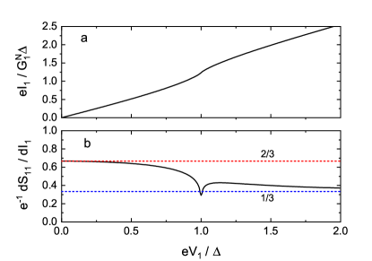
Figure 2: The current $I_{1}$ (69) in a diffusive contact 1 (a) and the corresponding differential Fano factor $e^{-1}dS_{11}/dI_{1}$ (b) (determined from Eqs. (69), (71)) as functions of the voltage bias $V_{1}$ at $T=0$. Here we define $G_{1}^{N}\equiv 1/R_{1}^{N}$.

The local current noise power in $r$-th NS contact with a diffusive boundary between metals is constructed analogously. It reads

$$S_{rr}=\frac{1}{R_{r}^{N}}\int_{|E|<\Delta}dE\left[f_{1}\left(\frac{E}{\Delta}\right)-f_{2}\left(\frac{E}{\Delta}\right)\right]w(n_{1}^{-},n_{1}^{+})$$

$$+\,\frac{1}{2R_{r}^{N}}\int_{-\infty}^{+\infty}dE\,f_{2}\left(\frac{E}{\Delta}\right)\,\big{[}w(n_{1}^{-},n_{1}^{-})+w(n_{1}^{+},n_{1}^{+})\big{]}$$

$$+\,\frac{1}{2R_{r}^{N}}\int_{|E|>\Delta}dE\bigg{\{}\left[f_{1}\left(\frac{E}{\Delta}\right)-\left(2-\frac{\Delta^{2}}{E^{2}}\right)f_{2}\left(\frac{E}{\Delta}\right)\right]$$

$$\times\,\big{[}w(n_{1}^{+},n_{S})+w(n_{1}^{-},n_{S})\big{]}$$

$$+\,2f_{2}\left(\frac{E}{\Delta}\right)\left(1-\frac{\Delta^{2}}{E^{2}}\right)w(n_{S},n_{S})\bigg{\}},$$ (71)

where the dimensionless function $f_{2}(x)$, defined as $f_{2}(x)=\int_{0}^{1}d\alpha\,g^{2}(x\Delta,\alpha)/4\alpha$, equals to

$$f_{2}(x) = \frac{\theta(1-|x|)}{2x^{2}}\left(\frac{1+x^{2}}{2|x|}\ln\frac{1+|x|}{1-|x|}-1\right)$$ (72)

$$+\,\theta(|x|-1)\frac{x^{2}}{2}\left(|x|\ln\frac{|x|+1}{|x|-1}-2\right).$$

The differential Fano factor $e^{-1}dS_{11}/dI_{1}$ following from the above results is displayed in Fig. 2b. At high voltage bias values it approaches the universal value $1/3$ expected for the normal metal, while at low bias $eV_{1}\ll\Delta$ the Fano factor becomes two times bigger due to the well-known charge doubling effect in the Andreev reflection regime Beenakker ; Sanquer ; Prober .

At this stage we have completed our preparations and now can turn to a discussion of non-local effects.

IV Non-local transport and noise in an NSN system

To begin with, let us we evaluate the non-local correction to the current flowing through the contact $r$ due to the presence of another contat $r^{\prime}$. We obtain

$$I_{r}=\frac{1}{2}\int\left(\frac{e}{\pi}\sum_{n}g_{r,n}(E)\right)(n_{r}^{-}-n_{r}^{+})$$

$$+\,\frac{1}{2e}\int dE\,G_{12}(E)(n_{r^{\prime}}^{-}-n_{r^{\prime}}^{+}),$$ (73)

where the non-local spectral conductance $G_{12}(E)$ reads GKZ

$$G_{12}(E)=\frac{e^{4}R_{0}^{S}}{\pi^{2}}\sum_{n,m}\bigg{[}\theta(\Delta-|E|)\frac{\Delta^{2}-E^{2}}{\Delta^{2}}$$

$$+\,\theta(|E|-\Delta)\frac{E^{2}-\Delta^{2}}{E^{2}}\bigg{]}g_{r,n}(E)g_{r^{\prime},m}(E).$$ (74)

Note that for simplicity in Eq. (73) we omitted disorder-induced corrections to the local junction conductance HN1 ; HN2 ; Tanaka which are insignificant for our present discussion.

One can also work out a full analytical expression for the cross-correlated noise of the contacts $S_{12}$. For the sake of completeness we present this rather lengthy expression in Appendix in Eq. (86). In the important limit of low voltages and temperatures, $eV_{1,2},T\ll\Delta$ one can derive a simple analytical expression,

$$S_{12}=G_{12}(0)\left[-4(2-\beta_{1}-\beta_{2})T-4\beta_{1}eV_{1}\coth\frac{eV_{1}}{T}\right.$$

$$\left.-\,4\beta_{2}eV_{2}\coth\frac{eV_{2}}{T}+\gamma_{+}e(V_{1}+V_{2})\coth\frac{e(V_{1}+V_{2})}{2T}\right.$$

$$\left.-\,\gamma_{-}e(V_{1}-V_{2})\coth\frac{e(V_{1}-V_{2})}{2T}\right],$$ (75)

where

$$\beta_{r}=\lim_{E\to 0}\frac{\sum_{n}A_{r,n}[1-A_{r,n}]}{\sum_{n}A_{r,n}}$$ (76)

are the effective Fano factors of the junctions in the regime where Andreev reflection dominates the transport properties, and the parameters $\gamma_{\pm}$ are defined as

$$\gamma_{\pm}=\frac{\sum_{n,m}A_{1,n}A_{2,m}\left[\frac{1-2A_{1,n}-2A_{2,m}+4A_{1,n}A_{2,m}}{\sqrt{A_{1,n}A_{2,m}}}\pm 1\right]}{\sum_{n,m}A_{1,n}A_{2,m}}.$$ (77)

Here the limit $E\to 0$ should be taken in the same way as in Eq. (76).

Eqs. (75)-(77) constitute an important generalization of our previous result GZ , where the assumption about equal transmissions of all conducting channels has been made. This assumption is lifted here, thus allowing one to analyze the results for a variety of transmission distributions in the contacts.

Figure 3: Zero temperature non-local conductance $\partial I_{1}/\partial V_{2}$ (determined by Eq. (82) with $E\to eV_{2}$) as a function of the bias voltage $V_{2}$.

In the tunneling limit $A_{1,n},A_{2,m}\ll 1$ one finds

$$\gamma_{+}=\gamma_{-}\equiv\gamma_{T}=\frac{\sum_{n,m}\sqrt{A_{1,n}A_{2,m}}}{\sum_{n,m}A_{1,n}A_{2,m}}.$$ (78)

Obviously in this regime we have $\gamma_{\pm}\gg 1$. Since in the other terms the prefactors are much smaller, one can keep only the terms $\propto\gamma_{\pm}$ in the expression (75), thereby reproducing the result Hekking

$$S_{12} = \gamma_{T}G_{12}(0)\left[e(V_{1}+V_{2})\coth\frac{e(V_{1}+V_{2})}{2T}\right.$$ (79)

$$\left.-\,e(V_{1}-V_{2})\coth\frac{e(V_{1}-V_{2})}{2T}\right].$$

The first and the second terms in the right-hand side of this formula are attributed respectively to CAR and EC processes. We observe that the noise cross-correlations remain positive, $S_{12}>0$, provided $V_{1}$ and $V_{2}$ have the same sign, and they turn negative, $S_{12}<0$, should $V_{1}$ and $V_{2}$ have different signs.

In the opposite limit of perfectly conducting channels in both junctions with $\tau_{1,n}=\tau_{2,m}=1$ one gets $\gamma_{+}=2$, $\gamma_{-}=0$, $\beta_{1}=\beta_{2}=0$. Hence, in this case we have GZ

$$S_{12}=G_{12}(0)\left[-8T+2e(V_{1}+V_{2})\coth\frac{e(V_{1}+V_{2})}{2T}\right].$$ (80)

This result is always positive at non-zero bias and low enough temperatures, indicating the importance of CAR processes in this limit. Note however, that in contrast to the tunnel limit (79), the last term in the Eq. (80) is not necessarily proportional to the CAR probability. Indeed, it may contain disorder averaged contributions of mixed processes involving both CAR and EC amplitudes Melin3 ; Ostrove , originating from the general expression for the noise in terms of the scattering matrixAD .

Provided superconductivity gets totally suppressed (i.e. we set $\Delta\to 0$), it is straightforward to verify that our general expression for the cross-correlated noise (86) reduces to the result GZ2

$$S_{12} = -\frac{R_{0}^{S}}{R_{1}^{N}R_{2}^{N}}\bigg{[}F_{1}eV_{1}\coth\frac{eV_{1}}{2T}+F_{2}eV_{2}\coth\frac{eV_{2}}{2T}$$ (81)

$$+\,(2-F_{1}-F_{2})2T\bigg{]},$$

where $F_{j}=\sum_{n}\tau_{j,n}(1-\tau_{j,n})/\sum_{n}\tau_{j,n}$ are the Fano factors of the contacts in the normal state. We also note that in the large bias limit $eV_{1},eV_{2}\gg\Delta$ Eq. (86) equals to the normal state result (81) plus voltage-independent excess noises related to both CAR and EC.

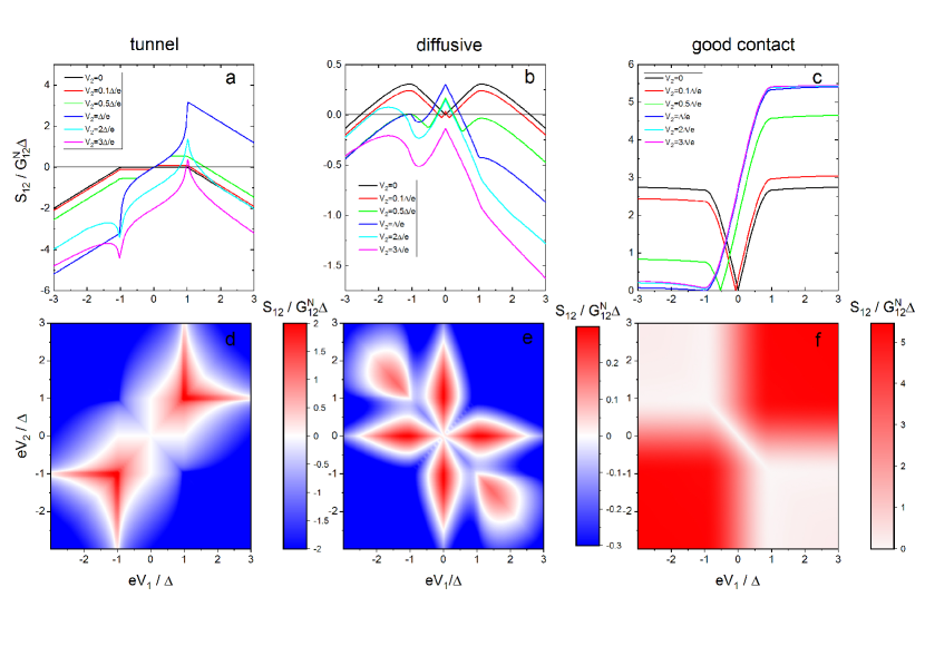
Figure 4: Non-local shot noise in an NSN structure at zero temperature, $T=0$, with various types of contacts: (a,d) tunnel contacts, Eq. (86) with $\tau_{1,n}=\tau_{2,m}=0.1$; (b,e) diffusive contacts, Eq. (83); (c,f) fully open contacts, Eq. (86) with $\tau_{1,n},\tau_{2,m}=1$ for all conducting channels. Graphs (a,b,c) show the dependence of the cross-correlated noise power $S_{12}$ on the bias voltage $V_{1}$ for several fixed values of $V_{2}$. Color plots (d,e,f) show the dependence of the noise cross correlations on both bias voltages $V_{1},V_{2}$ with red and blue colors indicating respectively positive and negative cross correlations.

Finally, let us analyze an important case of diffusive contacts. Making use of Eq. (74) and integrating over the transmission distribution (67), we arrive at the non-local spectral conductance in the form

$$G_{12}(E)=\frac{G_{12}^{N}}{4R_{1}^{N}R_{2}^{N}}\bigg{[}\theta(\Delta-|E|)\frac{\Delta^{2}-E^{2}}{E^{2}}$$

$$+\,\theta(|E|-\Delta)\frac{E^{2}-\Delta^{2}}{\Delta^{2}}\bigg{]}\left(\ln\left|\frac{|E|+\Delta}{|E|-\Delta}\right|\right)^{2},$$ (82)

where $G_{12}^{N}=R_{0}^{S}/(R_{1}^{N}R_{2}^{N})$ is the non-local conductance in the normal state. This result can be easily derived by applying Kirchhoff’s law to the equivalent circuit depicted in Fig. 1b and assuming that $R_{0}^{S}\ll R_{1,2}^{N}$. At $T=0$ the differential conductance $\partial I_{1}/\partial V_{2}$ exhibits the re-entrance effect (see Fig. 3). Namely, one finds that $\partial I_{1}/\partial V_{2}|_{V_{2}=0}=\lim_{V_{2}\to\infty}\partial I_{1}/\partial V_{2}=G_{12}^{N}$.

One can also work out a relatively simple analytical expression for $S_{12}$. After averaging over the distributions (67), the expression (86) reduces to the form

$$S_{12} = G_{12}^{N}\int dE\big{\{}-K_{1}(E/\Delta)\big{[}w(n_{1}^{-},n_{2}^{+})+w(n_{1}^{+},n_{2}^{-})-w(n_{1}^{-},n_{2}^{-})-w(n_{1}^{+},n_{2}^{+})\big{]}$$ (83)

$$+\,K_{2}(E/\Delta)\big{[}w(n_{1}^{-},n_{2}^{+})+w(n_{1}^{+},n_{2}^{-})+w(n_{1}^{-},n_{2}^{-})+w(n_{1}^{+},n_{2}^{+})\big{]}-K_{3}(E/\Delta)\big{[}w(n_{1}^{-},n_{1}^{+})+w(n_{2}^{-},n_{2}^{+})\big{]}$$

$$-\,K_{4}(E/\Delta)\big{[}w(n_{1}^{-},n_{S})+w(n_{1}^{+},n_{S})+w(n_{2}^{-},n_{S})+w(n_{2}^{+},n_{S})\big{]}$$

$$-\,K_{5}(E/\Delta)\big{[}w(n_{1}^{-},n_{1}^{-})+w(n_{1}^{+},n_{1}^{+})+w(n_{2}^{-},n_{2}^{-})+w(n_{2}^{+},n_{2}^{+})\big{]}+2K_{4}(E/\Delta)w(n_{S},n_{S})\big{\}}.$$

Here we defined five dimensionless functions $K_{j}(x)$. At $|x|<1$ (i.e. at $|E|<\Delta$) these functions read

$$K_{1}=x^{2}\left(f_{1}-f_{2}\right)^{2},\;\;K_{2}=(1-x^{2})f_{1}^{2}/4,$$

$$K_{3}=(1-x^{2})\left(f_{1}-f_{2}\right)f_{1},$$

$$K_{4}=0,\;\;K_{5}=(1-x^{2})f_{1}f_{2}/2,$$

where the functions $f_{1}(x)$ and $f_{2}(x)$ are defined, respectively, in Eqs. (70) and (72). For $|x|>1$ we have

$$K_{1}=\frac{\left(f_{1}-f_{2}\right)^{2}}{4x^{2}},\;K_{2}=-\frac{(x^{2}-1)f_{2}^{2}}{4x^{4}},\;K_{3}=0,$$

$$K_{4}=\frac{x^{2}-1}{2x^{2}}\left[f_{1}^{2}-2f_{1}f_{2}-\frac{f_{2}^{2}}{x^{2}}\right],\;K_{5}=\frac{(x^{2}-1)f_{1}f_{2}}{2x^{2}}.$$

The cross-correlated noise power for diffusive junctions (83) is plotted in Figs. 4b and 4e. For comparison, in the same Figure we have also displayed the result (86) in the tunneling limit (Figs. 4a and 4d) and for fully transparent junctions (Figs. 4c and 4f). For simplicity, in both these limiting cases we assume that all conducting channels in the junctions have the same transparency ($\tau=0.1$ for the tunnel limit and $\tau=1$ for fully open NS junctions). The dependence of $S_{12}$ on the bias voltage is asymmetric being very sensitive to the transparency of the junctions. Curves of a similar shape have also been obtained numerically Melin2 for a ballistic NSN structure within the scattering matrix approachAD . Interestingly, for good contacts $S_{12}$ remains positive even for $e|V_{1,2}|>\Delta$, although at high bias it becomes voltage independent, see Fig. 4c.

In the limit of low voltages and temperatures $eV_{1,2},T\lesssim\Delta$ the energy integrals in Eq. (83) can be performed analytically, and we obtain

$$S_{12} = G_{12}^{N}\bigg{[}-\frac{16}{3}T-\frac{4}{3}eV_{1}\coth\frac{eV_{1}}{T}-\frac{4}{3}eV_{2}\coth\frac{eV_{2}}{T}$$ (84)

$$+\,e(V_{1}+V_{2})\coth\frac{e(V_{1}+V_{2})}{2T}$$

$$+\,e(V_{1}-V_{2})\coth\frac{e(V_{1}-V_{2})}{2T}\bigg{]}.$$

Note that the last two terms in this expression for the cross-correlated current noise in NSN structures with diffusive contacts resemble those of the result (79) derived in the tunneling limit except the last term in Eq. (84) enters with the opposite sign as compared to that in Eq. (79). The expression (84) also follows from the general formula (75), since for diffusive junctions one finds $\beta_{1}=\beta_{2}=1/3$ and $\gamma_{\pm}=\pm 1$. Depending on the bias voltages $V_{1}$ and $V_{2}$ the cross-correlated noise (84) can take both positive and negative values, as it is illustrated in Fig. 4 b and e. We also stress that the results for the non-local noise power derived here for the case of diffusive contacts cannot be correctly reconstructed within a simple one-dimensional ballistic model Melin2 . Indeed, it is easy to check that, e.g., it order to get $\gamma_{\pm}=\pm 1$ within the latter model, for both barriers one should choose the same channel transmission value $\tau=2(\sqrt{2}-1)$. This choice, however, would then yield both subgap and overgap Fano factors, respectively $\beta_{1,2}$ and $F_{1,2}$, which do not correspond to the diffusive limit. Hence, e.g., the result in Eq. (84) cannot be recovered from the model Melin2 .

In summary, we have developed a detailed theory describing both non-local electron transport and non-local shot noise in three-terminal NSN hybrid structures with arbitrary distribution of transmissions for conducting channels in both NS junctions. Our theory does not employ any restrictions imposed on the electron energy and, hence, remains applicable at all voltage bias values and at any temperature. In our analysis we paid particular attention to the physically important limit of diffusive NS junctions, in which case a non-trivial behavior of non-local shot noise is recovered, exhibiting both positive and negative cross correlations depending on the bias voltages. Our predictions allow to better understand the process of Cooper pair splitting in NSN structures and are calling for their experimental verification.

Acknowledgements

This work was supported in part by RFBR Grant No. 18-02-00586, and by the Academy of Finland Centre of Excellence program (project 312057).

Appendix A

Performing the averaging outlined in Sec. II we derive the local part of the CGF (49) in the form

$${\cal F}_{r}(\chi_{r})={\rm tr}\,\ln\big{[}\check{I}_{rr}-\check{\Sigma}_{r}(\chi_{r})\langle\check{G}_{S,rr}\rangle\big{]}=t\sum_{n}\int\frac{dE}{2\pi}\ln\big{\{}1+A_{r,n}W(2\chi_{r},n_{r}^{+},n_{r}^{-})$$

$$+\,(C_{r,n}+D_{r,n})\big{[}W(\chi_{r},n_{r}^{+},n_{S})+W(-\chi_{r},n_{r}^{-},n_{S})\big{]}+\,(C_{r,n}-D_{r,n})^{2}W(\chi_{r},n_{r}^{+},n_{S})W(-\chi_{r},n_{r}^{-},n_{S})\big{\}},$$ (85)

where $W(\chi,n_{r},n_{r^{\prime}})=(e^{i\chi}-1)n_{r}(1-n_{r^{\prime}})+(e^{-i\chi}-1)(1-n_{r})n_{r^{\prime}}.$ The CGF (85) is equivalent to that derived in MK .

The general expression for the cross-correlated current noise $S_{12}$ which follows from our analysis in Sec. IV reads

$$S_{12}=\frac{e^{4}R_{0}^{S}}{\pi^{2}}\sum_{n,m}\int_{|E|<\Delta}dE\,\frac{\Delta^{2}-E^{2}}{\Delta^{2}}A_{1,n}A_{2,m}\bigg{\{}\bigg{[}\frac{(1-2A_{1,n})(1-2A_{2,m})}{\sqrt{A_{1,n}(0)A_{2,m}(0)}}-\frac{4E^{2}(1-A_{1,n})(1-A_{2,m})}{\Delta^{2}-E^{2}}\bigg{]}$$

$$\times\,\big{[}w(n_{1}^{-},n_{2}^{+})+w(n_{1}^{+},n_{2}^{-})-w(n_{1}^{-},n_{2}^{-})-w(n_{1}^{+},n_{2}^{+})\big{]}$$

$$+\,w(n_{1}^{-},n_{2}^{+})+w(n_{1}^{+},n_{2}^{-})+w(n_{1}^{-},n_{2}^{-})+w(n_{1}^{+},n_{2}^{+})-4\big{[}(1-A_{1,n})w(n_{1}^{-},n_{1}^{+})+(1-A_{2,m})w(n_{2}^{-},n_{2}^{+})\big{]}$$

$$-\,2A_{1,n}\left(w(n_{1}^{-},n_{1}^{-})+w(n_{1}^{+},n_{1}^{+})\right)-2A_{2,m}\left(w(n_{2}^{-},n_{2}^{-})+w(n_{2}^{+},n_{2}^{+})\right)\bigg{\}}$$

$$+\,\frac{e^{4}R_{0}^{S}}{\pi^{2}}\sum_{n,m}\int_{|E|>\Delta}dE\,\left(1-\frac{\Delta^{2}}{E^{2}}\right)g_{1,n}g_{2,m}\bigg{\{}-\frac{\Delta^{2}}{4(E^{2}-\Delta^{2})}\left(1-\frac{g_{1,n}}{2}\right)\left(1-\frac{g_{2,m}}{2}\right)\big{[}w(n_{1}^{-},n_{2}^{+})+w(n_{1}^{+},n_{2}^{-})$$

$$-\,w(n_{1}^{-},n_{2}^{-})-w(n_{1}^{+},n_{2}^{+})\big{]}-\frac{\Delta^{2}}{16E^{2}}g_{1,n}g_{2,m}\big{[}w(n_{1}^{-},n_{2}^{+})+w(n_{1}^{+},n_{2}^{-})+w(n_{1}^{-},n_{2}^{-})+w(n_{1}^{+},n_{2}^{+})\big{]}$$

$$+\,\left(\frac{\Delta^{2}}{8E^{2}}g_{1,n}g_{2,m}-\frac{1-g_{1,n}}{2}\right)\big{[}w(n_{1}^{-},n_{S})+w(n_{1}^{+},n_{S})-w(n_{S},n_{S})\big{]}+\left(\frac{\Delta^{2}}{8E^{2}}g_{1,n}g_{2,m}-\frac{1-g_{2,m}}{2}\right)$$

$$\times\,\big{[}w(n_{2}^{-},n_{S})+w(n_{2}^{+},n_{S})-w(n_{S},n_{S})\big{]}-\frac{g_{1,n}}{4}\big{[}w(n_{1}^{-},n_{1}^{-})+w(n_{1}^{+},n_{1}^{+})\big{]}-\frac{g_{2,m}}{4}\big{[}w(n_{2}^{-},n_{2}^{-})+w(n_{2}^{+},n_{2}^{+})\big{]}\bigg{\}}.$$ (86)

References

- (1) W. Belzig, F.K. Wilhelm, C. Bruder, G. Schön, and A.D. Zaikin, Superlatt. Microstruct. 25, 1251 (1999).
- (2) G. Deutscher and D. Feinberg, Appl. Phys. Lett. 76, 487 (2000).
- (3) G.B. Lesovik, T. Martin, and G. Blatter, Eur. Phys. J. B 24, 287 (2001).
- (4) P. Samuelsson, E.V. Sukhorukov, and M. Büttiker, Phys. Rev. Lett. 91, 157002 (2003).
- (5) F. Brange, O. Malkoc, and P. Samuelsson, Phys. Rev. Lett. 118, 036804 (2017).
- (6) G. Falci, D. Feinberg, and F.W.J. Hekking, Europhys. Lett. 54, 255 (2001).
- (7) A. Brinkman and A.A. Golubov, Phys. Rev. B 74, 214512 (2006).
- (8) M.S. Kalenkov and A.D. Zaikin, Phys. Rev. B 75, 172503 (2007).
- (9) M.S. Kalenkov and A.D. Zaikin, Phys. Rev. B 76, 224506 (2007).
- (10) J.P. Morten, A. Brataas, and W. Belzig, Phys. Rev. B 74, 214510 (2006).
- (11) D.S. Golubev and A.D. Zaikin, Phys. Rev. B 76, 184510 (2007).
- (12) A. Levy Yeyati, F.S. Bergeret, A. Martin-Rodero, and T.M. Klapwijk, Nat. Phys. 3, 455 (2007).
- (13) D.S. Golubev, M.S. Kalenkov, and A.D. Zaikin, Phys. Rev. Lett. 103, 067006 (2009).
- (14) D. Beckmann, H.B. Weber, and H. v. Löhneysen, Phys. Rev. Lett. 93, 197003 (2004).
- (15) S. Russo, M. Kroug, T. M. Klapwijk, and A. F. Morpurgo, Phys. Rev. Lett. 95, 027002 (2005).
- (16) P. Cadden-Zimansky and V. Chandrasekhar, Phys. Rev. Lett. 97, 237003 (2006).
- (17) L. Hofstetter, S. Csonka, J. Nygård, and C. Schönenberger, Nature (London) 461, 960 (2009).
- (18) L. G. Herrmann, F. Portier, P. Roche, A. Levy Yeyati, T. Kontos, and C. Strunk, Phys. Rev. Lett. 104, 026801 (2010).
- (19) A. Kleine, A. Baumgartner, J. Trbovic, D.S. Golubev, A.D. Zaikin, and C. Schönenberger, Nanotechnology 21, 274002 (2010).
- (20) J. Brauer, F. Hübler, M. Smetanin, D. Beckmann, and H. v. Löhneysen, Phys. Rev. B 81, 024515 (2010).
- (21) J. Schindele, A. Baumgartner, and C. Schönenberger, Phys. Rev. Lett. 109, 157002 (2012).
- (22) S. Kolenda, M.J. Wolf, D.S. Golubev, A.D. Zaikin, and D. Beckmann, Phys. Rev. B 88, 174509 (2013).
- (23) Ya.M. Blanter and M. Büttiker, Phys. Rep. 336, 1 (2000).
- (24) J. Börlin, W. Belzig, and C. Bruder, Phys. Rev. Lett. 88, 197001 (2002).
- (25) G. Bignon, M. Houzet, F. Pistolesi, F. W. J. Hekking, Europhys. Lett. 67, 110 (2004).
- (26) P. Samuelsson and M. Büttiker, Phys. Rev. Lett. 89, 046601 (2002).
- (27) R. Mélin, C. Benjamin, and T. Martin, Phys. Rev. B 77, 094512 (2008).
- (28) J.P. Morten, D. Huertas-Hernando, W. Belzig, and A. Brataas, Phys. Rev. B 78, 224515 (2008).
- (29) D.S. Golubev and A.D. Zaikin, Phys. Rev. B 82, 134508 (2010).
- (30) A. Freyn, M. Flöser, and R. Mélin, Phys. Rev. B 82, 014510 (2010).
- (31) M. Flöser, D. Feinberg, and R. Mélin, Phys. Rev. B 88, 094517 (2013).
- (32) C. Ostrove and L.E. Reichl, arXiv:1901.03766.
- (33) J. Wei and V. Chandrasekhar, Nat. Phys. 6, 494 (2010).
- (34) A. Das, Y. Ronen, M. Heiblum, D. Mahalu, A.V. Kretinin, and H. Shtrikman, Nat. Comm. 3, 1165 (2012).
- (35) J. C. Cuevas, A. Martin-Rodero, and A. Levy Yeyati, Phys. Rev. B 54, 7366 (1996).
- (36) A.F. Volkov, Phys. Rev. Lett. 74, 4730 (1995).
- (37) J.J.A. Baselmans, A.F. Morpurgo, B.J. van Wees and T.M. Klapwijk, Nature 397, 43 (1999).
- (38) R. Shaikhaidarov, A. F. Volkov, H. Takayanagi, V. T. Petrashov, and P. Delsing, Phys. Rev. B 62, R14649 (2000).
- (39) I.L. Aleiner, P.W. Brouwer, and L.I. Glazman, Phys. Rep. 358, 309 (2002).
- (40) G.E. Blonder, M. Tinkham, and T.M. Klapwijk, Phys. Rev. B 25, 4515 (1982).
- (41) B.A. Muzykantskii and D.E. Khmelnitskii, Phys. Rev. B 50, 3982 (1994).
- (42) M.P. Anantram and S. Datta, Phys. Rev. B 53, 16390 (1996).
- (43) O.N. Dorokhov, Solid State Comm. 51, 381 (1984).
- (44) M.J.M. de Jong and C.W.J. Beenakker, Phys. Rev. B 49, 16070 (1994).
- (45) X. Jehl, M. Sanquer, R. Calemczuk, and D. Mailly, Nature 405, 50 (2000).
- (46) A. A. Kozhevnikov, R. J. Schoelkopf, and D. E. Prober, Phys. Rev. Lett. 84, 3398 (2000).
- (47) F.W.J. Hekking and Yu.V. Nazarov, Phys. Rev. Lett. 71, 1625 (1993).
- (48) F.W.J. Hekking and Yu.V. Nazarov, Phys. Rev. B 49, 6847 (1994).
- (49) Y. Tanaka, A.A. Golubov, and S. Kashiwaya, Phys. Rev. B 68, 054513 (2003).
- (50) D.S. Golubev and A.D. Zaikin, Phys. Rev. B 85, 125406 (2012).