A new estimator for Weibull distribution parameters: Comprehensive comparative study for Weibull Distribution

Sahar Sadani
Email: s.sadani@gu.ac.ir
Department of Statistics, Faculty of Science, Golestan University, Gorgan, Iran.

Kamel Abdollahnezhad
Email: k.abdollahnezhad@gu.ac.ir
Department of Statistics, Faculty of Science, Golestan University, Gorgan, Iran.

Mahdi Teimouri
Email: teimouri@aut.ac.ir
Department of Mathematics and Statistics, Faculty of Science and Engineering, Gonbad Kavous University, Gonbad Kavous, Iran.

Vahid Ranjbar
Email: v.ranjbar@gu.ac.ir
Department of Statistics, Faculty of Science, Golestan University, Gorgan, Iran.

Abstract:
  Weibull distribution has received a wide range of applications in engineering and science. The utility and usefulness of an estimator is highly subject to the field of practitioner’s study. In practice users looking for their desired estimator under different setting of parameters and sample sizes. In this paper we focus on two topics. Firstly, we propose $U$-statistics for the Weibull distribution parameters. The consistency and asymptotically normality of the introduced $U$-statistics are proved theoretically and by simulations. Several of methods have been proposed for estimating the parameters of Weibull distribution in the literature. These methods include: the generalized least square type 1, the generalized least square type 2, the $L$-moments, the Logarithmic moments, the maximum likelihood estimation, the method of moments, the percentile method, the weighted least square, and weighted maximum likelihood estimation. Secondary, due to lack of a comprehensive comparison between the Weibull distribution parameters estimators, a comprehensive comparison study is made between our proposed $U$-statistics and above nine estimators. Based on simulations, it turns out that the our proposed $U$-statistics show the best performance in terms of bias for estimating the shape and scale parameters when the sample size is large.

Keywords:
Generalized least square; $L$-moment; $U$-statistic; Weibull distribution; Weighted least square; Weighted maximum likelihood;

1 Introduction

The Weibull distribution is one of the most commonly used distributions with a wide range of applications in some study fields such as: chemical engineering ([3], [22], and [41]), ecology [33], electrical engineering ([11] and [30]), food industry [4], mechanical engineering ([31] and [23]), telecommunications ([34] and [2]), wireless communications [28], economic ([27] and [7]), civil engineering ([26] and [1]), and seismology [15]. For further details on applications of the Weibull distribution, we refer the readers to Meeker and Escobar (1998), Murthy et al. (2004), and Dodson (2006). However, a comprehensive study has not been performed to compare the estimators. All comparative studies, to the best of our knowledge, have been devoted to compare the performance of the MLE with the estimators of another class. For example, Kanter (2015) made a comparison between least square estimators and the MLEs. The bias of the MLE for the Weibull distribution has been studied by Ross (1996), Watkins (1996) and Montanari et al. (1997). Seki and Yokoyama (1996) made a comparison between the MLE and a bootstrap estimator. Zhang et al. (2007) compared the estimation methods based on the Weibull probability plot. We also refer the readers to [10], [12], [17], [25], [36], and references therein. This is while estimators may have different appeals to different users. For example, the maximum likelihood estimator (MLE) that has attractive properties is biased and has not closed-form expression. This is while the practitioners from some fields may looking for an estimator that is unbiased or has closed-form expression. Also, user may prefer to use an estimator which works satisfactorily with sample of small size. Hence, a comparative study is needed to compare the performance of the known estimators under different situations. In this paper, we perform a comprehensive comparison study between ten class of estimators including: the generalized least square type 1 (GLS1), the generalized least square type 2 (GLS2), the $L$-moments (LM), the Logarithmic moments (MLM), the maximum likelihood estimation (MLE), the method of moments (MM), the percentile method (PM), the $U$-statistic, the weighted least square (WLS), and weighted maximum likelihood estimation (WMLE).

The structure of the paper is as follows. In Section 2, we derive $U$-statistic for the shape and scale parameters of the Weibull distribution. The known estimation methods are reviewed briefly in Section 3. A comparison between proposed estimator and the known ones as well as a real data illustration are given in Section 4.

2 $U$-statistics for the Weibull distribution parameters

The probability density function (pdf) and cumulative distribution function (cdf) of two-parameter Weibull distribution are, respectively, given by (Nelson, 1982; Johnson et al., 1994; Dodson, 2006):

$$f_{X}(x) =\frac{\alpha}{\beta}\left(\frac{x}{\beta}\right)^{\alpha-1}\exp\biggl{\{}-\left(\frac{x}{\beta}\right)^{\alpha}\biggr{\}},$$ (2.1)

$$F_{X}(x) =1-\exp\biggl{\{}-\left(\frac{x}{\beta}\right)^{\alpha}\biggr{\}},$$ (2.2)

for $x>0$, $\alpha>0$ and $\beta>0$. Here, $\alpha$ and $\beta$ are known as the shape and scale parameters. In the following we give $U$-statistics for the shape and scale parameters of the Weibull distribution. For this, a lemma given by the following is necessary. Hereafter, we write ${\cal{W}}(\alpha,\beta)$ to denote a Weibull distribution with pdf given in (2.1).

Lemma 2.1

Suppose $X_{1},X_{2}\mathop{\sim}\limits^{iid}{\cal{W}}(\alpha,\beta)$. Then

$$\min\{X_{1},X_{2}\}\mathop{=}\limits^{d}2^{-\frac{1}{\alpha}}X_{1}.$$ (2.3)

Proof: Define $Y=\min\{X_{1},X_{2}\}$. It follows that

$$F_{Y}(y)=1-\exp\biggl{\{}-2\left(\frac{y}{\beta}\right)^{\alpha}\biggr{\}},~{}~{}~{}y>0.$$ (2.4)

On the other hand, define $Z=2^{\frac{1}{\alpha}}X_{1}$. We have,

$$F_{Z}(y)=P(Z\leq y)=1-\exp\left\{-\left(\frac{y}{2^{-\frac{1}{\alpha}}\beta}\right)^{\alpha}\right\}.$$ (2.5)

Comparing the right-hand sides of (2.4) and (2.5), it turns out that $F_{Y}(y)=F_{Z}(y)$; for $y>0$, and so the result follows.

Theorem 2.1

Suppose $x_{1},x_{2},\dots,x_{n}$ are $n$ independent realizations from Weibull distribution with pdf given in (2.1). Then,

1. $$U_{\alpha}={\dbinom{n}{2}}^{-1}\sum_{1\leq i<j\leq n}H_{1}(x_{i},x_{j}),$$

   in which

   $$H_{1}(x_{i},x_{j})=\frac{\log\min\{x_{i},x_{j}\}}{\log 2}-\frac{\log x_{i}+\log x_{j}}{2\log 2},$$

   is $U$-statistic for $1/\alpha$.

2. $$U_{\sigma}={\dbinom{n}{2}}^{-1}\sum_{1\leq i<j\leq n}H_{2}(x_{i},x_{j}),$$

   in which

   $$H_{2}(x_{i},x_{j})=\biggl{(}1+\frac{\psi(1)}{\log 2}\biggl{)}\frac{\log x_{i}+\log x_{j}}{2}-\frac{\psi(1)}{\log 2}\log\min\{x_{i},x_{j}\},$$

   where $\psi(1)=-0.57721566$ is $U$-statistic for $\log\sigma$.

Proof:

1. By applying log-transformation to the both sides of (2.3), we have

   $$\frac{1}{\alpha}=\frac{\log\min\{X_{1},X_{2}\}-\log{{X}}_{1}}{\log 2}.$$ (2.6)

   The right-hand side of (2.6) can be used to construct a symmetric kernel as

   $$H_{1}(x_{1},x_{2})=\frac{\log x_{1}+\log x_{2}}{2\log 2}-\frac{\log\min\{x_{1},x_{2}\}}{\log 2}.$$ (2.7)

   It is easy to see that $\text{E}\bigl{(}H_{1}({X}_{1},{X}_{2})\bigr{)}=1/\alpha$. To guarantee the asymptotic normality of the introduced $U$-statistics for $1/\alpha$ with kernel (2.7), it is necessary to show that $\text{Var}\bigl{(}E\left(H_{1}({X}_{1},{X}_{2})\big{|}{X}_{1}\right)\bigr{)}$ is finite. For this, it suffices to show that $\text{Var}\bigl{(}H_{1}({{X}}_{1},{{X}}_{2})\bigr{)}$ is finite. To begin, we note that $X,X_{1},X_{2}\mathop{\sim}\limits^{iid}{\cal{W}}(\alpha,\beta)$. Since $\min\{X_{1},X_{2}\}\mathop{=}\limits^{d}2^{-\frac{1}{\alpha}}X_{1}$, it follows that

   $$\text{Var}(\log X) =\text{Var}\left(\log\min\{X_{1},X_{2}\}\right).$$ (2.8)

   Also, suppose $X$, $Y$, and $Z$ are given arbitrary random variables. Generally, we cannot conclude that if $X\mathop{=}\limits^{d}Y$, then $\text{Cov}\bigl{(}X,Z\bigr{)}=\text{Cov}\bigl{(}Y,Z\bigr{)}$. But, here, elementary statistical manipulations reveal that if we define $X=\log\min\{X_{1},X_{2}\}$, $Y=\log X_{1}$, and $Z=\log X_{1}+\log X_{2}$, then

   $$\text{Cov}\left(\log\min\{X_{1},X_{2}\},\log X_{1}+\log X_{2}\right) =\text{Cov}\left(\log X_{1},\log X_{1}+\log X_{2}\right).$$ (2.9)

   Now, using (2.8), we can write

   $$\text{Var}\bigl{(}H_{1}({{X}}_{1},{{X}}_{2})\bigr{)}=\frac{\text{Var}\log X}{\log^{2}2}+\frac{\text{Var}\log X}{2\log^{2}2}-\frac{\text{Cov}\bigl{(}\log\min\{X_{1},X_{2}\},\log X_{1}+\log X_{2}\bigr{)}}{\log^{2}2}.$$ (2.10)

   Applying property (2.9) to the right-hand side of (2.10), we obtain

   $$\text{Var}\bigl{(}H_{1}({{X}}_{1},{{X}}_{2})\bigr{)}\leq\frac{\text{Var}(\log X)}{2\log^{2}2}.$$

   It is easy to check that $\text{Var}(\log X)=\psi(1,1)/\alpha^{2}$ where $\psi(n,x)=\partial^{n}\psi(x)/\partial x^{n}$ and $\psi(x)=\partial\log\Gamma(x)/\partial x$. The asymptotic normality of $U_{\alpha}$ follows since

   $$\text{Var}\bigl{(}H_{1}({{X}}_{1},{{X}}_{2})\bigr{)}\leq\frac{\psi(1,1)}{2\alpha^{2}\log^{2}2}<\infty.$$

2. It is not hard to check that $\text{E}(\log X)=\log\beta+\frac{\psi(1)}{\alpha}$ where $\psi(1)=-0.5772157$. Define $H_{2}(x_{1},x_{2})$ as

   $$H_{2}(x_{1},x_{2}) =\frac{\log x_{1}+\log x_{2}}{2}-\psi(1)H_{1}(x_{1},x_{2})$$

   $$=\frac{\log x_{1}+\log x_{2}}{2}\biggl{(}1-\frac{\psi(1)}{\log 2}\biggr{)}+\frac{\psi(1)}{\log 2}\log\min\{x_{1},x_{2}\}.$$ (2.11)

   It is easy to see that $\text{E}\bigl{(}H_{1}({{X}}_{1},{{X}}_{2})\bigr{)}=\log\beta$. Asymptotic normality of the introduced $U$-statistics for $\log\beta$ with kernel (2) holds if we prove $\text{Var}\bigl{(}E\left(H_{2}({X}_{1},{X}_{2})\big{|}{X}_{1}\right)\bigr{)}<\infty$ or equivalently $\text{Var}\bigl{(}H_{1}({{X}}_{1},{{X}}_{2})\bigr{)}<\infty$. We eliminate the proof since kernels $H_{1}(x_{1},x_{2})$ and $H_{2}(x_{1},x_{2})$ have similar structure.

3 Known estimators for the Weibull distribution

Here, we review briefly almost all of known estimation methods for the Weibull distribution.

3.1 Maximum likelihood estimation (MLE)

There is no closed-form expression for MLEs of the Weibull distribution parameters. It is asymptotically normal and efficient for large sample sizes. Many attempts have been made to compute or modify the MLEs of the Weibull distribution parameters. Cohen and Whitten (1982) considered a modified MLE involving complicated numerical computations. Dodson (2006) derived the MLE for the shape parameter graphically. The MLE of the shape parameter is computed as the root of the equation, see [29]

$$\displaystyle\frac{n}{\alpha}-\sum_{i=1}^{n}\log x_{i}-n\log\beta+\sum_{i=1}^{n}\biggl{(}\frac{x_{i}}{\beta}\biggr{)}^{\alpha}\log\biggl{(}\frac{x_{i}}{\beta}\biggr{)},$$

and the MLE of the scale parameter is given by

$$\widehat{\beta}_{MLE}=\left(\frac{{\sum_{i=1}^{n}{x_{i}^{\alpha}}}}{n}\right)^{\frac{1}{\alpha}}.$$

It can be seen that $\widehat{\beta}_{MLE}$ depends on $\alpha$ and also that $\widehat{\alpha}_{MLE}$ must be computed numerically.

3.2 Weighted Maximum likelihood (WMLE)

It is known that MLEs are generally biased. To reduce the bias rate in the case of the Weibull distribution, the weighted maximum likelihood estimators (WMLE) have been proposed in [19]. Suppose $x_{1},x_{2},\ldots,x_{n}$ is a random sample from cdf given in (2.2), then the WMLEs of the shape and scale parameters are given by

$${\hat{\alpha}}_{WMLE} =\arg\min\limits_{\alpha}~{}\biggl{(}\frac{W_{2}}{\alpha}+\frac{1}{n}\log x_{i}-\frac{\sum_{i=1}^{n}x_{i}^{\alpha}\log x_{i}}{\sum_{i=1}^{n}x_{i}^{\alpha}}\biggr{)}^{2},$$

$${\hat{\beta}}_{WMLE} =\biggl{(}\frac{1}{nW_{1}}\sum_{i=1}^{n}x_{i}^{\alpha}\biggr{)}^{\frac{1}{\alpha}},$$

where the weights $W_{1}$ and $W_{2}$ are given by

$$W_{1} =-\frac{1}{n}\sum_{i=1}^{n}\log(1-F(X_{i})),$$

$$W_{2} =\frac{\sum_{i=1}^{n}\log\bigl{(}1-F(X_{i})\bigr{)}\log\bigl{(}-\log(1-F(X_{i}))\bigr{)}}{\sum_{i=1}^{n}\log(1-F(X_{i}))}-\frac{1}{n}\sum_{i=1}^{n}\log\bigl{(}-\log(1-F(X_{i}))\bigr{)}.$$

Although the sampling distribution of the $W_{1}$ is gamma with shape parameter $n$ and scale parameter $1/n$, but the sampling distribution of the $W_{2}$ is not known. In practice, both of random variables $W_{1}$ and $W_{2}$ are replaced by their central quantities such as mean, median, or geometric mean. Here, we use the median of $W_{1}$ and $W_{2}$ since they yield the best performance, see [5]. For this, in a comprehensive Monte Carlo simulation, we derive the median of $W_{1}$ and $W_{2}$ for different levels of $\alpha$ (from 0.5 to 5 by 0.2) and small sample size $n$ (including 5, 10, 15, 30, 50, 100, …, 200). We note that as $n$ tends to $\infty$, both WMLE and MLE approaches give the same results.

3.3 Generalized and weighted least square (GLS and WLS)

The parameter estimation using least square approach is common in the statistical literature. For Pareto, log-logistic and Weibull distributions we refer the readers to [20], [18], [24], [42], [38], and [43]. Suppose $x_{(1)}\leq x_{(2)}\leq\dots\leq x_{(n)}$ are the ordered realizations from Weibull distribution with pdf given in (2.2). We can see that the following regression model holds.

$$y_{(i)}=\log\beta+\frac{1}{\alpha}\log\bigl{(}-\log(1-F(x_{(i)}))\bigr{)},$$ (3.1)

for $i=1,\dots,n$ where $y_{(i)}=\log x_{(i)}$. The quantity $F(x_{(i)})$, in the right-hand side of regression model (3.1), is replaced by $\frac{i}{n+1}$ or $\frac{i-0.3}{n+0.4}$, see [37], [38], and [21]. Since the sample $x_{(i)}$ is ordered, the dependent variable $y_{(i)}$ is also ordered. Therefore the variance of dependent variable is not of the form $\sigma^{2}$I, see [20]. To tackle this issue the generalized least square (GLS) technique is proposed, see [9]. The GLS estimate, i.e., $\hat{\boldsymbol{\beta}}_{GLS1}=(\log\hat{\beta},1/\hat{\alpha})^{T}$ is given by

$$\hat{\boldsymbol{\beta}}_{GLS1}=\bigl{(}X^{T}V^{-1}X\bigr{)}X^{T}V^{-1}Y,$$ (3.2)

where $Y=(\log x_{(1)},\log x_{(2)},\dots,\log x_{(n)})^{T}$,

$$X=\begin{pmatrix}1&\log\bigl{(}-\log(1-\hat{F}(x_{(1)}))\bigr{)}\\ \vdots&\vdots\\ 1&\log\bigl{(}-\log(1-\hat{F}(x_{(n)}))\bigr{)}\end{pmatrix},$$

and

$$V=\begin{pmatrix}v_{11}&\dots&v_{1n}\\ \vdots&\vdots&\vdots\\ v_{n1}&\dots&v_{nn}\end{pmatrix},$$

for

$$v_{ij}=\frac{i}{(n+1-i)}\frac{1}{\log(n+1-i)-\log(n+1)}\frac{1}{\log(n+1-j)-\log(n+1)};~{}~{}~{}~{}~{}~{}i\leq j.$$

The second type of GLS estimate, i.e.,

$$\hat{\boldsymbol{\beta}}_{GLS2}=\bigl{(}Z^{T}V^{-1}X\bigr{)}Z^{T}V^{-1}Y,$$ (3.3)

can be constructed if we replace $X$ with $Z$ as

$$Z=\begin{pmatrix}1&\log\bigl{(}-\log(1-\hat{F}(x_{(1)}))\bigr{)}-0.5-\frac{\log(1-\hat{F}(x_{(1)}))}{\bigl{(}(1-\hat{F}(x_{(1)}))\log(1-\hat{F}(x_{(1)}))\bigr{)}^{2}}\\ \vdots&\vdots\\ 1&\log\bigl{(}-\log(1-\hat{F}(x_{(n)}))\bigr{)}-0.5-\frac{\log(1-\hat{F}(x_{(n)}))}{\bigl{(}(1-\hat{F}(x_{(n)}))\log(1-\hat{F}(x_{(n)}))\bigr{)}^{2}}\end{pmatrix}.$$

We note that $\hat{\boldsymbol{\beta}}_{GLS2}=(\log\hat{\beta},1/\hat{\alpha})^{T}$ and $\hat{F}(x_{(i)})=\frac{i}{n+1}$. The weighted least square (WLS) estimate are also given by

$$\hat{\boldsymbol{\beta}}_{WLS}=\bigl{(}X^{T}W^{-1}X\bigr{)}X^{T}W^{-1}Y,$$ (3.4)

where $\hat{\boldsymbol{\beta}}_{WLS}=(\log\hat{\beta},1/\hat{\alpha})^{T}$ and $W$ is a diagonal matrix whose entries are $v_{11},\dots,v_{nn}$, see [20].

3.4 $L$-moment (LM)

The $L$-moments have their origin in works by Hosking (1990) and Elamir and Seheult (2003). By equating the sample $L$-moment to the population counterpart gives the $L$-moment estimate. The $r$-th $L$-moment of Weibull distribution with pdf (2.1) is given by:

$$\mu_{r}^{L}=\frac{\beta}{r}\Gamma\left(\frac{1}{\alpha}+1\right)\sum\limits_{k=0}^{r-1}{(-1)^{k}}C_{k}^{r-1}(r-k)C_{r-k}^{r}\sum\limits_{j=0}^{r-k-1}C_{j}^{r-k-1}\frac{\displaystyle(-1)^{j}}{\displaystyle(k+j+1)^{1/\alpha+1}},$$

where $\alpha>0$, $\beta>0$, $r=1,2,\ldots$, and $C_{i}^{n}$ denotes the binomial coefficient $n!/(i!(n-i)!)$, see [16]. So the first and the second $L$-moments are given by $\mu_{1}^{L}=\beta\Gamma\left({1/\alpha+1}\right)$ and $\mu_{2}^{L}=\beta\Gamma\left({1/\alpha+1}\right)\bigl{(}{1-{\displaystyle 2^{-1/\alpha}}}\bigr{)}$, respectively. The first two sample $L$-moments are:

$$m_{1}^{L}=\frac{1}{n}\sum\limits_{i=1}^{n}{X_{i:n}}=\overline{X},$$

and

$$m_{2}^{L}=\frac{2}{n(n-1)}\sum\limits_{i=1}^{n}{(i-1)X_{i:n}-\overline{X}}.$$

Now, equating $\mu_{1}^{L}$ and $\mu_{2}^{L}$ with $m_{1}^{L}$ and $m_{2}^{L}$, respectively, the $L$-moments of $\alpha$ and $\beta$ are obtained as:

$$\widehat{\alpha}_{LM}=-\frac{\displaystyle\ln(2)}{\displaystyle\ln\left(1-m_{2}^{L}/m_{1}^{L}\right)},$$

and

$$\widehat{\beta}_{LM}=\frac{\displaystyle m_{1}^{L}}{\displaystyle\Gamma\left({1/\widehat{\alpha}_{LM}+1}\right)}.$$

3.5 Method of logarithmic moment (MLM)

The log-moment estimates of the shape and scale parameters of Weibull distribution with cdf (2.2) are given by (see [40], [29], and [8])

$$\widehat{\alpha}_{MLM}=\sqrt{\frac{\displaystyle\pi^{2}}{\displaystyle 6S^{2}}},$$ (3.5)

and

$$\widehat{\beta}_{MLM}=\exp\big{\{}M_{1}-\psi(1)/\widehat{\alpha}_{MLM}\big{\}},$$ (3.6)

where $S^{2}$ and $M_{1}$ are the sample variance and the mean of log-transformed data, respectively. Also $\psi(1)=-0.5772156$. It can be shown that (3.5) and (3.6) are both asymptotically unbiased and consistent, see [29].

3.6 Percentile method (PM)

The quantile of a Weibull distribution with cdf (2.2) is

$$x_{p}=\beta\left[{-\ln(1-p)}\right]^{1/\alpha},$$

where $0<p<1$, see [29] and [8]. Using $p=1-\exp(-1)\cong 0.632$, one can construct percentile-based estimators for $\alpha$ and $\beta$ as

$$\hat{\alpha}_{PM}=\left({\frac{\displaystyle\ln[-\ln(1-p)]}{\displaystyle\ln\left(x_{p}\right)-\ln\left(x_{0.632}\right)}}\right),$$ (3.7)

and

$$\hat{\beta}_{PM}=x_{1-\exp(-1)},$$ (3.8)

respectively, where $0<x_{p}<x_{0.632}$. The suggested values for $p$ are 0.15 (see [39]) and 0.31, see ([32] and [14]). Statistical tools show that percentile-based estimators are, in general, asymptotically normal and unbiased, see [40].

3.7 Method of moments (MM)

Moment-based estimators of a given population are obtained by equating the population moments to their sample counterparts and solving the resulting equations. The moment-based estimators for the Weibull distribution suffers from numerical computations, see [6]. Also, these estimators are not efficient. The $r$-th non-central moment for the Weibull distribution is ([40]; [29]; [8]):

$$\mu_{r}=\beta^{r}\Gamma\left(r/\alpha+1\right).$$

Equating the mean and variance ($\mu_{1}$ and $\mu_{2}-\mu_{1}^{2}$) with the sample counterparts ($\overline{X}$ and $S^{2}$), the moment-based estimator of the shape parameter $\widehat{\alpha}_{MM}$, is root of the equation

$$\frac{\displaystyle\Gamma(1+2/\alpha)}{\displaystyle\Gamma^{2}(1+1/\alpha)}+\frac{\displaystyle S^{2}}{\displaystyle\overline{X}}-1=0,$$

and the moment-based estimator of the scale parameter is

$$\widehat{\beta}_{MM}=\frac{\displaystyle\overline{X}}{\displaystyle\Gamma\left({1/\widehat{\alpha}_{MM}+1}\right)}.$$

4 Performance comparisons

This section has two parts. In the first part, we compare the performances of estimators introduced in Section 2 and 3 through simulation. Second part devoted to an illustration in which all estimators are applied to a set of real data.

4.1 Simulation study

Here, we perform a Monte Carlo simulation to compare the performance of the $U$-statistic, MLE, WMLE, GLS1, GLS2, WLS, LM, MLM, PM, and MM. For this aim, we compare the bias and root of mean squared error (RMSE).

For computing the bias we adopt small sizes of sample including 5, 10, 30, and two levels for shape and scale parameters as: (0.5, 0.5), (2.5, 0.5), (0.5, 2.5), and (2.5, 2.5). The results after computing the bias are given in Tables 1-2. Also the bias of $U$-statistic, MLE, GLS1, GLS2, WLS, and LM are given for large sizes of sample including 1000 and 4000. The corresponding results are given in Tables 3-4 for shape and scale parameters, respectively.

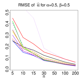
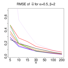
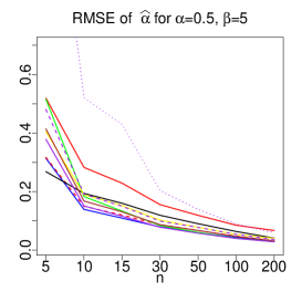
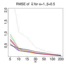
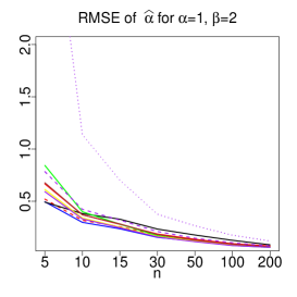
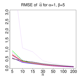
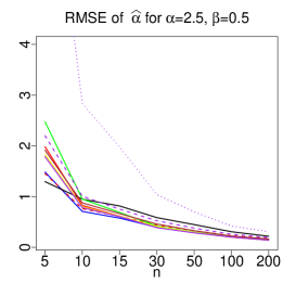
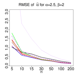
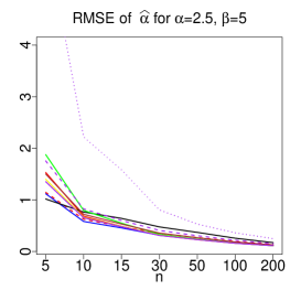
Figure 1: RMSE of the shape parameter estimator, $\hat{\alpha}$ for different levels of $\alpha$ and $\beta$ under small sample size scenario, i.e., $n=$5, 10, 15, 30, 50, 100, and 200. The used color scheme are: the black solid curve for the GLS2, blue solid curve for the WLS, brown solid curve for the $U$-statistic, green solid curve for the MLE, solid red curve for the MM, dashed red curve for the GLS1, purple solid curve for the WMLE, dotted purple curve for the PM, dashed purple curve for the MLM, and yellow solid curve for LM.

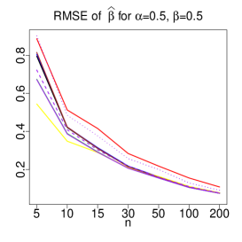
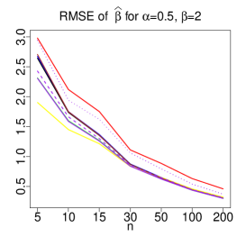
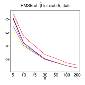
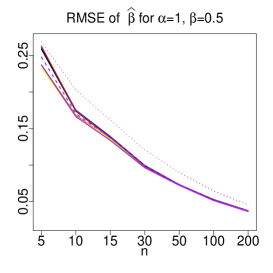
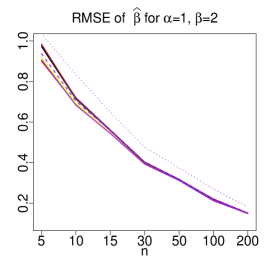
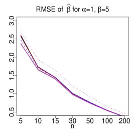
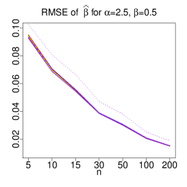
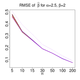
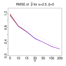
Figure 2: RMSE of the scale parameter estimator, $\hat{\beta}$ for different levels of $\alpha$ and $\beta$ under small sample size scenario, i.e., $n=$5, 10, 15, 30, 50, 100, and 200. The used color scheme are: the black solid curve for the GLS2, blue solid curve for the WLS, brown solid curve for the $U$-statistic, green solid curve for the MLE, solid red curve for the MM, dashed red curve for the GLS1, purple solid curve for the WMLE, dotted purple curve for the PM, dashed purple curve for the MLM, and yellow solid curve for LM.

For computing the RMSE, we choose the sample sizes as: 5, 10, 15, 30, 50, 100, and 200. Comparisons are performed for different levels of the shape ($\alpha$=0.5, 1, and 2.5) and the scale ($\beta$=0.5, 2, and 5) parameters. We used a 7-color scheme to distinguish between competitors through Figures 1-2 as follows. The brown for the $U$-statistic, green for the MLE, purple for the WMLE, dashed red for the GLS1, black for the GLS2, blue for the WLS, dashed purple for the MLM, dotted purple for the PM, solid red for the MM, and yellow solid curve for LM. The results for computing the RMSE are given in Figures 1-2.

4.1.1 Comparison results for the bias

According to the bias of the shape parameter estimator $\hat{\alpha}$ for small sizes 5, 10, and 30, the following conclusions can be made from Table 1.

1. GLS2 , WLS, and WMLE give the best performances for $n=5$, $n=10$, and $n=30$, respectively.

2. WMLE shows the best performance next to the WLS and GLS1.

3. PM gives the worst performance.

4. When $\alpha$ is small (say $\alpha=0.5$), the MM gives the worst performance next to the GLS2.

5. When $\alpha$ is large (say $\alpha=2.5$) and $n\geq 15$, the GLS2 gives the worst performance.

6. WMLE outperforms the LM.

7. WMLE and $U$-statistic outperform the MLE.

8. $U$-statistic shows better performance than the MLE, MLM, MM, and PM.

The following observations can be made from Table 2 for bias of the scale parameter estimator $\hat{\beta}$ for small sizes 5, 10, and 30.

1. WMLE and MLE give almost the same performances.

2. When $\alpha$ is small (say $\alpha=0.5$), the MM gives the worst performance.

3. When $\alpha$ is small, the LM gives the best performance.

4. The GLS2, GLS1, and WLS show the same performances.

5. MLM outperforms GLS2, GLS1, and WLS.

6. When $\alpha$ is large (say $\alpha=2.5$), the PM shows the worst performance.

7. The GLS2, GLS1, and WLS outperforms the $U$-statistic for $n=5,10$.

The following observations can be made from Tables 3-4 for bias of the shape parameter estimator $\hat{\beta}$ for large sizes 1000 and 4000.

1. $U$-statistic gives the best performance for estimating the shape and scale parameters.

2. GLS1 shows the worst performance for estimating the shape and scale parameters.

We note that for bias analysis when sample sizes are large, the MLM, PM, and MM have been eliminated by competitions since the show weak performances. Also, since MLE and WMLE show the same performances, the WMLE has been removed by competitions.

4.1.2 Comparison results for RMSE

The following observations can be made from Figure 1 for RMSE of the shape parameter estimator $\hat{\alpha}$.

1. The PM gives the worst performance.

2. When $n=5$ the GLS2 gives the best performance.

3. When $n=5$ the GLS2 gives the best performance.

4. The WGLS gives the best performance next to the GLS1.

5. The WMLE outperforms the LM and $U$-statistic.

6. The MLM shows better performance than the MLE for sample size (say $n\leq 10$).

The following observations can be made from Figure 2 for RMSE of the scale parameter estimator $\hat{\beta}$.

1. The PM gives the worst performance.

2. When $\alpha$ is small (say $\alpha\leq 0.5$), the MM gives the worst performance.

3. When $\alpha$ is not small (say $\alpha\geq 1$), the PM gives the worst performance.

4. When $\alpha$ is small (say $\alpha\leq 0.5$) and $n\leq 15$, the LM gives the best performance.

4.2 Real data illustration

Here, we apply all reviewed methods introduced in Sections 2 and 3 to a set of real data involving by lifetimes in years reported by [13, p. 17]. Data are shown in Table 5. To implement these techniques, programs have been written in R environment, see [35]. In order to compare the performance of estimators presented in the Section 2 and 3, we employed the Kolmogorov-Smirnov (KS) and Cramer-Von Mises (CVM) distances which are given by

$$\text{KS}=\max\limits_{\boldsymbol{1\leq i\leq n}}\max\left\{\frac{i}{n}-F_{X}\bigl{(}x_{(i)}\bigr{)},F_{X}\bigl{(}x_{(i)}\bigr{)}-\frac{i-1}{n}\right\},$$

and

$$\text{CVM}=\frac{1}{12n}+\sum\limits_{i=1}^{n}\biggl{[}\frac{2i-1}{2n}-F_{X}\bigl{(}x_{(i)}\bigr{)}\biggr{]}^{2},$$

where $n$ is the sample size, $x_{(i)}$; for $i=1\dots,n$, is the $i$-th ordered observed value and $F_{X}(.)$ is the distribution function of two-parameter Weibull distribution defined in (2.2). The following observations can be made from Table 6.

1. The WLS shows the best performance in the sense of both criteria KS and CVM.

2. The MLM shows the best performance in the sense of CVM criterion next to the WLS.

3. The PM shows the best performance in the sense of KS criterion next to the WLS.

Table 1: Bias of shape parameter estimators for samples of small size.

	n=5
	parameters level
Method	($\alpha=0.5$, $\beta=0.5$)	($\alpha=0.5$, $\beta=2.5$)	($\alpha=2.5$, $\beta=0.5$)	($\alpha=2.5$, $\beta=2.5$)
$U$-Statistic	0.346	0.383	1.890	1.415
MLE	0.422	0.473	2.453	1.813
WMLE	0.299	0.340	1.764	1.309
GLS1	0.266	0.292	1.420	1.106
GLS2	0.249	0.255	1.261	1.025
WLS	0.252	0.283	1.449	1.082
LM	0.331	0.359	1.798	1.353
MLM	0.405	0.443	2.203	1.645
PM	1.199	1.699	8.597	7.132
MM	0.450	0.476	1.971	1.452
	n=10
	parameters level
Method	($\alpha=0.5$, $\beta=0.5$)	($\alpha=0.5$, $\beta=2.5$)	($\alpha=2.5$, $\beta=0.5$)	($\alpha=2.5$, $\beta=2.5$)
$U$-Statistic	0.181	0.189	0.865	0.713
MLE	0.193	0.195	0.914	0.776
WMLE	0.161	0.162	0.756	0.636
GLS1	0.159	0.164	0.765	0.608
GLS2	0.196	0.195	0.966	0.749
WLS	0.148	0.146	0.697	0.572
LM	0.193	0.191	0.781	0.649
MLM	0.205	0.216	0.999	0.817
PM	0.546	0.553	2.491	2.334
MM	0.279	0.278	0.806	0.664
	n=30
	parameters level
Method	($\alpha=0.5$, $\beta=0.5$)	($\alpha=0.5$, $\beta=2.5$)	($\alpha=2.5$, $\beta=0.5$)	($\alpha=2.5$, $\beta=2.5$)
$U$-Statistic	0.071	0.074	0.383	0.301
MLE	0.078	0.079	0.410	0.332
WMLE	0.074	0.073	0.379	0.309
GLS1	0.085	0.084	0.425	0.342
GLS2	0.121	0.119	0.588	0.468
WLS	0.077	0.076	0.385	0.311
LM	0.099	0.110	0.393	0.315
MLM	0.095	0.096	0.493	0.400
PM	0.184	0.191	1.045	0.867
MM	0.150	0.149	0.386	0.313

Table 2: Bias of scale parameter estimators for samples of small size.

	n=5
	parameters level
Method	($\alpha=0.5$, $\beta=0.5$)	($\alpha=0.5$, $\beta=2.5$)	($\alpha=2.5$, $\beta=0.5$)	($\alpha=2.5$, $\beta=2.5$)
$U$-Statistic	0.816	2.717	0.094	0.481
MLE	0.674	2.318	0.091	0.460
WMLE	0.673	2.315	0.091	0.459
GLS1	0.809	2.686	0.094	0.481
GLS2	0.795	2.641	0.093	0.477
WLS	0.806	2.670	0.094	0.479
LM	0.544	1.909	0.093	0.469
MLM	0.723	2.431	0.092	0.468
PM	0.903	2.943	0.099	0.508
MM	0.927	2.983	0.092	0.463
	n=10
	parameters level
Method	($\alpha=0.5$, $\beta=0.5$)	($\alpha=0.5$, $\beta=2.5$)	($\alpha=2.5$, $\beta=0.5$)	($\alpha=2.5$, $\beta=2.5$)
$U$-Statistic	0.424	1.752	0.067	0.337
MLE	0.389	1.608	0.066	0.329
WMLE	0.387	1.596	0.066	0.329
GLS1	0.385	1.652	0.067	0.337
GLS2	0.421	1.744	0.067	0.336
WLS	0.423	1.752	0.067	0.338
LM	0.349	1.455	0.067	0.332
MLM	0.409	1.663	0.067	0.335
PM	0.485	1.948	0.077	0.393
MM	0.513	2.129	0.066	0.331
	n=30
	parameters level
Method	($\alpha=0.5$, $\beta=0.5$)	($\alpha=0.5$, $\beta=2.5$)	($\alpha=2.5$, $\beta=0.5$)	($\alpha=2.5$, $\beta=2.5$)
$U$-Statistic	0.215	0.866	0.038	0.186
MLE	0.207	0.841	0.037	0.187
WMLE	0.207	0.842	0.037	0.188
GLS1	0.214	0.869	0.038	0.191
GLS2	0.215	0.869	0.038	0.191
WLS	0.215	0.874	0.038	0.191
LM	0.201	0.830	0.037	0.188
MLM	0.218	0.857	0.038	0.195
PM	0.257	1.060	0.045	0.227
MM	0.284	1.110	0.037	0.202

Table 3: Bias of shape parameter estimators for samples of large size.

	n=1000
	parameters level
Method	($\alpha=0.5$, $\beta=0.5$)	($\alpha=0.5$, $\beta=2.5$)	($\alpha=2.5$, $\beta=0.5$)	($\alpha=2.5$, $\beta=2.5$)
GLS1	0.005193	0.003696	0.018966	0.008460
WLS	0.005025	0.003351	0.017895	0.006642
GLS2	-0.005167	-0.002230	-0.016367	-0.007867
MLE	-0.004958	-0.002026	-0.017401	-0.005958
LM	0.004229	0.002091	0.016958	0.005620
U-Statistic	0.003600	0.001065	0.013052	0.003600
	n=4000
	parameters level
Method	($\alpha=0.5$, $\beta=0.5$)	($\alpha=0.5$, $\beta=2.5$)	($\alpha=2.5$, $\beta=0.5$)	($\alpha=2.5$, $\beta=2.5$)
GLS1	0.002892	0.976e-03	0.009939	0.003492
WLS	0.002632	0.764e-03	0.009614	0.002632
GLS2	-0.002260	-6.088e-04	-0.009609	-0.002260
MLE	-0.002372	-9.705e-04	-0.009305	-0.002372
LM	0.001498	-7.164e-04	-0.007535	0.002498
U-Statistic	0.001253	2.018e-04	-0.004859	0.001253

Table 4: Bias of scale parameter estimators for samples of large size.

	n=1000
	parameters level
Method	($\alpha=0.5$, $\beta=0.5$)	($\alpha=0.5$, $\beta=2.5$)	($\alpha=2.5$, $\beta=0.5$)	($\alpha=2.5$, $\beta=2.5$)
GLS1	0.006450	0.013542	0.006873	-0.014509
WLS	0.004087	0.011946	0.006442	0.013873
GLS2	0.004891	0.011840	0.005900	0.011489
MLE	0.005883	0.011700	-0.005236	0.010988
LM	0.006123	0.010598	-0.006468	0.012319
U-Statistic	0.003323	0.007526	0.005378	0.009353
	n=4000
	parameters level
Method	($\alpha=0.5$, $\beta=0.5$)	($\alpha=0.5$, $\beta=2.5$)	($\alpha=2.5$, $\beta=0.5$)	($\alpha=2.5$, $\beta=2.5$)
GLS1	0.001854	0.005237	1.968e-03	0.002354
WLS	0.001263	0.003971	1.879e-03	0.001263
GLS2	0.001495	0.003879	1.807e-03	0.001495
MLE	0.001382	0.004028	1.748e-03	0.001382
LM	0.001545	-0.003890	1.651e-03	0.001845
U-Statistic	0.000552	-0.002518	1.029e-03	0.000552

Table 5: Lifetime data (in year)

30.20	36.55	25.11	39.35	27.57	25.91	31.50	29.24	18.39	16.65	21.85	24.88
31.61	18.74	19.63	28.98	11.10	21.66	22.41	26.04	25.07	23.48	28.21	25.21
25.12	27.76	23.47	23.51	24.39	21.93	37.63	20.32	28.17	24.66	30.13	21.42
17.21	19.98	33.09	16.04	17.96	19.57	22.91	25.69	23.47	16.91	27.20	27.23

Table 6: Estimation results after fitting two-parameter Weibull distribution to the lifetime data.

	Estimated parameters		goodness-of-fit measures
Method	$\hat{\alpha}$	$\hat{\beta}$	KS	CVM
$U$-statistic	5.1575	26.8644	0.0934	0.0591
MLE	4.5922	26.9452	0.0920	0.0713
WMLE	4.5141	26.9370	0.0906	0.0744
GLS1	4.7548	26.9926	0.0971	0.0721
GLS2	4.3035	26.9788	0.0904	0.0926
WLS	4.7099	26.6979	0.0777	0.0482
LM	4.9512	26.9055	0.0939	0.0609
MLM	5.3119	26.7771	0.0889	0.0529
PM	5.9767	25.8461	0.0867	0.0622
MM	4.9150	26.9169	0.0942	0.0621

5 Conclusion

We have introduced $U$-statistics for shape and scale parameters of two-parameter Weibull distribution. Asymptotic normality and consistency of the new estimators have been proved. Furthermore, a comprehensive Monte Carlo study have been carried out to compare the performance of the known estimators of the two-parameter Weibull distribution parameters. Since different estimators may appeal different users for different levels of sample size and parameters levels, a list of comparisons have been made in the paper for choosing desired estimator. Many facts can be concluded from this study, among them our results are the followings.

• for small sizes of samples the weighted least square (WLS) approach gives the best performance in the sense of bias.

• shape estimator based on method of weighted least square (WLS) gives the best performance root of mean squared error (RMSE).

• shape estimator based on method of percentile gives the worst performance in terms of RMSE.

• shape and scale estimators based on $U$-statistic show the best performances in the sense of bias for large sample sizes.

• shape and scale estimators based on generalized least square type-I (GLS1) approach show the worst performances in the sense of bias for large sample sizes.

References

- [1] J. M. Arenas, J. J. Narbón, and C. Alía. Optimum adhesive thickness in structural adhesives joints using statistical techniques based on weibull distribution. International Journal of Adhesion and Adhesives, 30(3):160–165, 2010.
- [2] W. Buller, B. Wilson, L. Van Nieuwstadt, and J. Ebling. Statistical modelling of measured automotive radar reflections. In Instrumentation and Measurement Technology Conference (I2MTC), 2013 IEEE International, pages 349–352. IEEE, 2013.
- [3] Y. J. Chiang, C. Shih, C. Lin, and Y. Tseng. Examination of tyre rubber cure by weibull distribution functions. International Journal of Materials and Product Technology, 20(1-3):210–219, 2004.
- [4] O. Corzo, N. Bracho, A. Pereira, and A. Vásquez. Weibull distribution for modeling air drying of coroba slices. LWT-Food Science and Technology, 41(10):2023–2028, 2008.
- [5] D. Cousineau. Nearly unbiased estimators for the three-parameter weibull distribution with greater efficiency than the iterative likelihood method. British Journal of Mathematical and Statistical Psychology, 62:167–191, 2009.
- [6] G. Cran. Moment estimators for the 3-parameter weibull distribution. IEEE Transactions on Reliability, 37(4):360–363, 1988.
- [7] A. Diaconu. Weibull distribution as a model for growth/decline in product sales. Metalurgia International, 14:184–185, 2009.
- [8] B. Dodson. The Weibull analysis handbook. ASQ Quality Press, 2006.
- [9] R. M. Engeman and T. J. Keefe. On generalized least squares estimation of the weibull distribution. Communications in Statistics-Theory and Methods, 11(19):2181–2193, 1982.
- [10] O. L. Gebizlioglu, B. Şenoğlu, and Y. M. Kantar. Comparison of certain value-at-risk estimation methods for the two-parameter weibull loss distribution. Journal of Computational and Applied Mathematics, 235(11):3304–3314, 2011.
- [11] A. Genc, M. Erisoglu, A. Pekgor, G. Oturanc, A. Hepbasli, and K. Ulgen. Estimation of wind power potential using weibull distribution. Energy Sources, 27(9):809–822, 2005.
- [12] U. Genschel and W. Q. Meeker. A comparison of maximum likelihood and median-rank regression for weibull estimation. Quality Engineering, 22(4):236–255, 2010.
- [13] N. Glick. Breaking records and breaking boards. The American Mathematical Monthly, 85(1):2–26, 1978.
- [14] K. M. Hassanein. Percentile estimators for the parameters of the weibull distribution. Biometrika, 58(3):673–676, 1971.
- [15] T. Hasumi, T. Akimoto, and Y. Aizawa. The weibull–log weibull distribution for interoccurrence times of earthquakes. Physica A: Statistical Mechanics and its Applications, 388(4):491–498, 2009.
- [16] J. R. Hosking. L-moments: analysis and estimation of distributions using linear combinations of order statistics. Journal of the royal statistical society. Series B (Methodological), pages 105–124, 1990.
- [17] A. Hossain and W. Zimmer. Comparison of estimation methods for weibull parameters: complete and censored samples. Journal of statistical computation and simulation, 73(2):145–153, 2003.
- [18] W.-L. Hung. Weighted least-squares estimation of the shape parameter of the weibull distribution. Quality and Reliability Engineering International, 17(6):467–469, 2001.
- [19] J. Jacquelin. Generalization of the method of maximum likelihood. IEEE Transactions on Electrical Insulation, 28(1):65–72, 1993.
- [20] Y. M. Kantar. Generalized least squares and weighted least squares estimation methods for distributional parameters. REVSTAT-Statistical Journal, 13(3):263–282, 2015.
- [21] Y. M. Kantar and V. Yildirim. Robust estimation for parameters of the extended burr type iii distribution. Communications in Statistics-Simulation and Computation, 44(7):1901–1930, 2015.
- [22] L. Kuo-Chao, W. Keng-Tung, C. Chien-Song, et al. A new study on combustion behavior of pine sawdust characterized by the weibull distribution. Chinese Journal of Chemical Engineering, 17(5):860–868, 2009.
- [23] V. Lavanya, G. S. Rao, and B. Bidikar. Fast fading mobile channel modeling for wireless communication. Procedia Computer Science, 85:777–781, 2016.
- [24] H.-L. Lu, C.-H. Chen, and J.-W. Wu. A note on weighted least-squares estimation of the shape parameter of the weibull distribution. Quality and Reliability Engineering International, 20(6):579–586, 2004.
- [25] C. R. Mohan, A. V. Rao, and G. V. S. R. Anjaneyulu. Comparison of least square estimators with rank regression estimators of weibull distribution-a simulation study. Journal of Statistics, 20(1), 2013.
- [26] G. Muraleedharan, A. Rao, P. Kurup, N. U. Nair, and M. Sinha. Modified weibull distribution for maximum and significant wave height simulation and prediction. Coastal Engineering, 54(8):630–638, 2007.
- [27] S. Nadarajah and S. Kotz. The modified weibull distribution for asset returns. Quantitative Finance, 6(6):449–449, 2006.
- [28] K. M. Noga and B. Pałczyńska. Overview of fading channel modeling. International Journal of Electronics and Telecommunications, 56(4):339–344, 2010.
- [29] L. Norman, S. Kotz, and N. Balakrishnan. Continuous univariate distributions, 1994.
- [30] P. Pascual. Morchella esculenta (morel) rehydration process modeling. Journal of food engineering, 72:346–353, 2006.
- [31] K. Raghunathan, V. Subramaniam, and V. Srinivasamoorthy. Studies on the tensile characteristics of ring and rotor yarns using modified weibull distribution. 2002.
- [32] T. Seki and S. Yokoyama. Robust parameter-estimation using the bootstrap method for the 2-parameter weibull distribution. IEEE Transactions on Reliability, 45(1):34–41, 1996.
- [33] T. V. Stankova and T. M. Zlatanov. Modeling diameter distribution of austrian black pine (pinus nigra arn.) plantations: a comparison of the weibull frequency distribution function and percentile-based projection methods. European journal of forest research, 129(6):1169–1179, 2010.
- [34] P. Surendran, J.-H. Lee, S. J. Ko, et al. Parameter optimization of uwb srr system performance in weibull clutter environment. organization, 7(2), 2014.
- [35] R. C. Team. R: A language and environment for statistical computing. r foundation for statistical computing, vienna, austria. 2013, 2014.
- [36] M. Teimouri, S. M. Hoseini, and S. Nadarajah. Comparison of estimation methods for the weibull distribution. Statistics, 47(1):93–109, 2013.
- [37] M. Tiryakioğlu and D. Hudak. On estimating weibull modulus by the linear regression method. Journal of Materials Science, 42(24):10173–10179, 2007.
- [38] J. M. Van Zyl and R. Schall. Parameter estimation through weighted least-squares rank regression with specific reference to the weibull and gumbel distributions. Communications in Statistics-Simulation and Computation, 41(9):1654–1666, 2012.
- [39] F. Wang and J. B. Keats. Improved percentile estimation for the two-parameter weibull distribution. Microelectronics Reliability, 35(6):883–892, 1995.
- [40] N. Wayne. Applied life data analysis, 1982.
- [41] M. A. Wood, B. Gunderson, A. Xia, X. Zhou, V. Padmanabhan, and K. A. Ellenbogen. Temporal patterns of ventricular tachyarrhythmia recurrences follow a weibull distribution. Journal of cardiovascular electrophysiology, 16(2):181–185, 2005.
- [42] L. Zhang, M. Xie, and L. Tang. On weighted least squares estimation for the parameters of weibull distribution. In Recent Advances in Reliability and Quality in Design, pages 57–84. Springer, 2008.
- [43] L. Zhang, M. Xie, and L. C. Tang. A study of two estimation approaches for parameters of weibull distribution based on wpp. Reliability Engineering & System Safety, 92(3):360–368, 2007.