The Optimal Approximation Factor in Density Estimation

Abstract

Consider the following problem: given two arbitrary densities $q_{1},q_{2}$ and a sample-access to an unknown target density $p$, find which of the $q_{i}$’s is closer to $p$ in total variation.

A remarkable result due to Yatracos shows that this problem is tractable in the following sense: there exists an algorithm that uses $O(\epsilon^{-2})$ samples from $p$ and outputs $q_{i}$ such that with high probability, $TV(q_{i},p)\leq 3\cdot\mathsf{opt}+\epsilon$, where $\mathsf{opt}=\min\{TV(q_{1},p),TV(q_{2},p)\}$. Moreover, this result extends to any finite class of densities ${\cal Q}$: there exists an algorithm that outputs the best density in ${\cal Q}$ up to a multiplicative approximation factor of 3.

We complement and extend this result by showing that: (i) the factor 3 can not be improved if one restricts the algorithm to output a density from ${\cal Q}$, and (ii) if one allows the algorithm to output arbitrary densities (e.g. a mixture of densities from ${\cal Q}$), then the approximation factor can be reduced to 2, which is optimal. In particular this demonstrates an advantage of improper learning over proper in this setup.

We develop two approaches to achieve the optimal approximation factor of $2$: an adaptive one and a static one. Both approaches are based on a geometric point of view of the problem and rely on estimating surrogate metrics to the total variation. Our sample complexity bounds exploit techniques from Adaptive Data Analysis.

1 Introduction

We study the problem of agnostic distribution learning whereby a learner is given i.i.d. samples from an unknown distribution $p$ and needs to choose, among a set ${\cal Q}$ of candidate distributions, the one that is closest to $p$. This problem formulation immediately raises several questions. The first one is how to define close-ness between probability distributions. Here we will argue that the total variation metric is a natural choice. The second one is what assumptions are made on $p$. We choose the so called agnostic or robust case which means that we are not making any assumption. The last one is whether the best thing to do for the learner is to return an element of ${\cal Q}$ (this is called the proper case), or to possibly produce a distribution which is not a member of ${\cal Q}$ (this is the improper case) but is guaranteed to be competitive with respect to the best member of ${\cal Q}$.

Our study will focus on the information-theoretic limits of the problem, which means that we will not be concerned with the computational complexity of the learner and will only consider what, in theory, is the best achievable performance of a learner as a function of the size of the candidate class ${\cal Q}$ and the number $m$ of samples from $p$ that it has access to.

1.1 Why Total Variation?

The total variation metric, defined for two probability measures $p,q$ on ${\cal X}$ as

$$TV(p,q):=\sup_{A\subset{\cal X}}\left|p(A)-q(A)\right|\,,$$ (1)

has the nice property of being a proper metric. Additionally it has the natural interpretation of measuring the largest discrepancy in the measure assigned to the same event by the two different measures. And while it thus looks like an $L_{\infty}$ metric (when viewing a probability measure as a map from subsets of ${\cal X}$ to $[0,1]$), it also can be rewritten as an $L_{1}$ norm: if $p$ and $q$ have densities $dp$ and $dq$ respectively (or probability mass function when ${\cal X}$ is finite/countable),

$$TV(p,q)=\frac{1}{2}\left\|dp-dq\right\|_{1}\,,$$ (2)

as well as an optimal coupling:

$$TV(p,q)=\inf_{(Y,Z):Y\sim p,Z\sim q}\mathbb{P}(Y\neq Z)\,.$$ (3)

Note that there is a large literature about density estimation in the $L_{2}$ metric (as opposed to $L_{1}$). However, $L_{2}$ is a less natural way of measuring the distance between densities because it lacks invariance with respect to the choice of the reference measure on the domain. This may not be an issue when considering real-valued distributions where the Lebesgue measure is the canonical choice, but when working on high-dimensional or general domains, this dependency is not necesssarily desirable (for more details, see Chapter 6.5 in the book by Devroye and Lugosi (2001)).

Another classical choice is to use the Kullback-Leibler divergence, however $KL(q,p)$ has the down-side of being defined only when $q$ is absolutely continuous with respect to $p$ and in a setting like the one we are considering where we do not wish to assume anything about the target distribution, this cannot be guaranteed. Even if one were to consider $KL(p,q)$ instead, then one would be restricted to considering models that put mass on all points of the domain and the Kullback-Leibler distance could be dominated by the points of very low $q$ probability.

Compared to those other two choices, total variation has the benefit of being invariant, bounded and being a metric. We refer the reader to Chapter 6 in the book by Devroye and Lugosi (2001) for a discussion regarding the advantages of total variation and a detailed comparison with other natural similarity measures.

Of course, there are other possible choices such as the Hellinger divergence or others, and it would be an interesting question to extend the current study to those.

1.2 Why Agnostic?

A basic classification of machine learning problems separates between realizable and agnostic learning. In the realizable case one assumes that the target distribution $p$ belongs to a prespecified class ${\cal Q}$ which is known to the algorithm, and in the agnostic case one usually does not assume anything about the target distribution $p$ but rather extends the goal of learning to so that the output distribution $q$ is competitive with the best distribution in ${\cal Q}$ (i.e. the one which is closest to $p$).

In this work we focus on the agnostic case. Nevertheless, a sensible setting to keep in mind is the “almost realizable” case in which the distance between $p$ and ${\cal Q}$ is small. Such scenarios may occur in contexts where one has a strong prior about the target distribution, but would like to remain resilient/robust against small fluctuations and thus to avoid realizability assumptions.

1.3 Why Improper?

Another basic classification in machine learning problems distinguishes between proper and improper learning. In the proper case the algorithm always outputs a distribution $q\in{\cal Q}$ whereas in the improper case it may output arbitrary distribution (in both cases the goal remains the same, namely to compete with the best distribution in ${\cal Q}$). While at a first glance it may seem strange to consider the improper case, it turns out that in many cases improperness is beneficial (e.g. boosting is inherently improper (Schapire and Freund, 2012); in multiclass classification some classes can only be learned improperly (Daniely and Shalev-Shwartz, 2014)). The main results in this paper manifest another setting in which improper learning is provably stronger than proper learning.

1.4 Is this problem too hard?

While the total variation is a natural metric with strong guarantees, at a first glance it may seem impossible to use in such an abstract distribution learning setting: imagine that the class ${\cal Q}$ contains just two distributions $q_{1},q_{2}$, and let $p$ denote the target distribution. Then, a natural empirical-risk-minimization-like approach would be to estimate both distances $\mathsf{TV}(q_{1},p),\mathsf{TV}(q_{2},p)$ from a large enough i.i.d. sample drawn from $p$ and output the minimizer. The problem with this approach is that estimating $\mathsf{TV}(\cdot,p)$ requires $\Omega(\lvert{\cal X}\rvert)$ samples from $p$ (see e.g. Jiao et al. (2018)). In particular, if ${\cal X}$ is infinite (say ${\cal X}=\mathbb{R}$) then it is impossible to do it with a finite sample complexity.

However, perhaps surprisingly, despite the impossibility of estimating the total variation one can still find an approximate minimizer of it (even when ${\cal X}$ is infinite!). A more detailed survey of relevant results is given in Section 1.6 below.

1.5 Problem Definition

Let ${\cal X}$ be a domain and let $\Delta({\cal X})$ denote the set of all probability distributions over ${\cal X}$. We assume that either (i) ${\cal X}$ is finite in which case $\Delta({\cal X})$ is identified with the set of $\lvert{\cal X}\rvert$-dimensional probability vectors, or (ii) ${\cal X}={\mathbb{R}}^{d}$ in which case $\Delta({\cal X})$ is the set of Borel probability measures.

Let ${\cal Q}\subseteq\Delta({\cal X})$ be a set of distributions. We focus on the case where ${\cal Q}$ is finite and denote its size by $n$. Let $\alpha>0$, we say that ${\cal Q}$ is $\alpha$-learnable if there is a (possibly randomized) algorithm $A$ such that for every $\epsilon,\delta>0$ there is a finite sample complexity bound $m=m(\epsilon,\delta)$ such that for every target distribution $p\in\Delta({\cal X})$, if $A$ receives as input at least $m$ independent samples from $p$ then it outputs a distribution $q$ such that

$$\mathsf{TV}(p,q)\leq\alpha\cdot\mathsf{opt}+\epsilon,$$

with probability at least $1-\delta$, where $\mathsf{opt}=\min_{q\in{\cal Q}}\mathsf{TV}(p,q)$ and $\mathsf{TV}(p,q)=\sup_{A\subseteq{\cal X}}\{p(A)-q(A)\}$ is the total variation distance. We say that ${\cal Q}$ is properly $\alpha$-learnable if it is $\alpha$-learnable by a proper algorithm; namely an algorithm that always outputs $q\in{\cal Q}$. The function $m=m(\epsilon,\delta)$ is called the sample complexity of the algorithm.

Sample complexity.

Note that if ${\cal X}$ is finite then any class of distribution is $\alpha$-learnable for $\alpha=1$ with sample complexity $O(\lvert{\cal X}\rvert/\epsilon^{2})$ (because this many samples suffice to estimate $p(A)$ for every $A\subseteq{\cal X}$, which allows to estimate its total variation distance to each $q\in{\cal Q}$). Therefore, when ${\cal X}$ is finite, we consider ${\cal Q}$ to be $\alpha$-learnable only if its sample complexity depends efficiently on $\lvert{\cal X}\rvert$, namely $\mathsf{poly}\log(\lvert{\cal X}\rvert)$ (note that $\log\lvert{\cal X}\rvert$ is the bit-complexity of representing each sample in the input and therefore $\mathsf{poly}\log\lvert{\cal X}\rvert$ means polynomial in the input size).

1.6 Previous Related Work

Density estimation has been studied since more than a century ago, for textbook introductions see e.g. (Devroye and Gyorfi, 1985; Devroye and Lugosi, 2001; Diakonikolas, 2016). A significant portion of works considered this problem when ${\cal Q}$ is some specific class of distributions such as mixtures of gaussians (e.g. Kalai et al. (2012); Diakonikolas et al. (2017, 2018a); Kothari et al. (2018); Ashtiani et al. (2018b, a)), histograms (e.g. Pearson (1895); Lugosi and Nobel (1996); Devroye and Lugosi (2004); Chan et al. (2014); Diakonikolas et al. (2018b)), and more. For a fairly recent survey see (Diakonikolas, 2016).

This work concerns arbitrary classes ${\cal Q}$ and the only assumption we make is that ${\cal Q}$ is finite. The factor 3 upper bound in the proper case was derived by Yatracos (1985) using the elegant and simple idea of Yatracos’ sets (also referred to as Schaffe’s sets by Devroye and Lugosi (2001)). Devroye and Lugosi (2001) extended Yatracos’ idea and also gave a factor 2 lower bound for his algorithm. Mahalanabis and Stefankovic (2008) improved the lower bound to 3 and extended it to a more general family of proper algorithms. Mahalanabis and Stefankovic (2008) also showed that in the case of $n=2$ distributions, the exists a randomized proper algorithm, which achieves a factor $2$. approximation A lower bound of factor 2 for arbitrary (possibly improper) algorithms follows from the work Chan et al. (2014) (see section 1.7). Devroye and Lugosi (2001) point out in their book the absence of universal methods other than Yatracos’ which achieve a constant approximation factor; this comment inspired the current work.

1.7 Main Results

Theorem 1 (Upper bound - improper case).

Every finite class of distributions ${\cal Q}$ is $\alpha$-learnable with $\alpha=2$.

We prove Theorem 1 and provide explicit sample complexity bounds in Section 3.

Theorem 2 (Lower bound - proper case).

For every $\alpha<3$ there is a class ${\cal Q}$ of size $2$ that is not properly $\alpha$-learnable.

We prove Theorem 2 and provide explicit sample complexity bounds in Section 5.

Tightness of Theorem 1.

The factor $\alpha=2$ in Theorem 1 in general can not be improved. This follows from Chan et al. (2014) (Theorem 7) which demonstrates a class ${\cal Q}$ of distributions over $\{1,\ldots,N\}$ such that any (possibly improper) algorithm that $\alpha$-learns this class with $\alpha<2$ requires some $\Omega(\sqrt{N})$ samples. Note that in their Theorem statement the class ${\cal Q}$ is infinite, but a closer inspection of their proof reveals that it needs only to contain two distributions, and so their lower bound already applies for $\lvert{\cal Q}\rvert=2$.

Proofs overview.

Our approach for the lower bound is a variant of the proof in Chan et al. (2014) and boils down to using a tensorized version of Le Cam’s method together with a birthday paradox kind of argument.

For the upper bound, we introduce two methods, a static and an adaptive one, both of which are based on the observation that once we find a distribution $q$ so that $\mathsf{TV}(q,q_{i})\leq\mathsf{TV}(p,q_{i})+\epsilon$ for every $q_{i}\in{\cal Q}$ the result follows by the triangle inequality (see Lemma 3). The static method can be viewed as a direct extension of Yatracos’ ideas as we also construct a family of functions of finite VC dimension and estimate the corresponding surrogate variational metric (see Equation (4)). Note however that our construction and analysis are more complex and rely on a careful inspection of barycenters with respect to the total variation metric.

The adaptive method, which could apply to other probability metrics than $\mathsf{TV}$ proceeds in steps: it maintains lower bounds $z_{i}\leq\mathsf{TV}(p,q_{i})$ and, at each step, increases one of them by at least $\epsilon$ until there exists a distribution $q$ such that $\mathsf{TV}(q,q_{i})\leq z_{i}+\epsilon$ for all $i$. Given that $\mathsf{TV}$ is bounded by $1$, this implies that the algorithm terminates after $|{\cal Q}|/\epsilon$ steps. The crux of the algorithm is in the implementation of each step. To this end we use the minimax theorem applied to $\min_{q}\mathsf{TV}(q,q_{i})$ (since $\mathsf{TV}$ is a supremum) to find functions $f_{i}$ so that some linear combination of the numbers $|\mathbb{E}[f_{i}(q)]-\mathbb{E}[f_{i}(q_{i})]|-z_{i}-\epsilon$ is positive for any distribution $q$. Applying this result for $q=p$ implies that estimating $\mathbb{E}[f_{i}(p)]$ will allow us to improve at least one of our lower bounds.

1.8 Open Questions and Future Research

The main result in this paper is the determination of the optimal approximation factor in density estimation and the development of universal algorithmic approaches to achieve it.

One central issue that remains open concerns sample complexity. Our current sample complexity upper bounds are either linear in $\lvert{\cal Q}\rvert$ or based on rather sophisticated techniques from adaptive data analysis which includes dependencies on $\log\lvert{\cal X}\rvert$. For comparison, Yatracos’ proper algorithm which achieves factor 3 has a clean sample complexity of $\frac{\log\lvert{\cal Q}\rvert}{\epsilon^{2}}$. It would be interesting to determine whether the factor $2$ can be achieved with a similar sample complexity.

We list below other possible suggestions for future research:

• Mahalanabis and Stefankovic (2008) consider the case of ${\cal Q}=\{q_{1},q_{2}\}$ and provide a randomized proper algorithm which outputs $q_{i}\in{\cal Q}$ such that $\mathbb{E}[\mathsf{TV}(q_{i},p)]\leq 2\mathsf{opt}+o(1)$ (see Theorem 10 in (Mahalanabis and Stefankovic, 2008)). Can this result be extended to arbitrary finite ${\cal Q}$?

• Is it the case that any (possibly infinite) class ${\cal Q}$ that is $\alpha$-learnable for some $\alpha$ is $\alpha$-learnable for $\alpha=2$? E.g. assume that the family of Yatracos’ sets of ${\cal Q}$ has a finite VC dimension (so ${\cal Q}$ is properly $\alpha$-learnable for $\alpha=3$). Is ${\cal Q}$ $\alpha$-learnable for $\alpha=2$?

• Our result remains valid if we replace the total variation with any IPM metric. How about $f$-divergences? Is there a natural characterization of all $f$-divergences for which every finite ${\cal Q}$ can be $\alpha$-learned for some constant $\alpha<\infty$?

2 Preliminaries

An assumption.

Some of our arguments exploit the Minimax Theorem for zero-sum games (von Neumann, 1928). Therefore, we will assume a setting (i.e. the domain ${\cal X}$ and the set of distributions ${\cal Q}\subseteq\Delta({\cal X})$) in which this theorem is valid. Alternatively, one could state explicit assumptions such as finiteness or forms of compactness under which it is known that the Minimax Theorem holds. However, we believe that the presentation benefits from avoiding such explicit technical assumptions and simply assuming the Minimax Theorem as an “axiom” in the discussed setting.

Standard notation.

We use $[N]$ to denote the set $\{1,\ldots,N\}$. For two vectors $u,v\in{\mathbb{R}}^{n}$ let $u\leq v$ denote the statement that $u_{i}\leq v_{i}$ for every $i$. Denote by $e_{i}$ the standard basis vector whose $i$’th coordinate is $1$ and its other coordinates are $0$ and by $1_{n}$ the vector $(1,\ldots,1)\in{\mathbb{R}}^{n}$.

We use standard notations for asymptotics such as $O,o,\Omega,\omega,\Theta$. We may also sometimes use $\tilde{O}$ or $\tilde{\Omega}$ to hide logarithmic factors. E.g. $f=\tilde{O}(g)$ if $f=O(g\log^{c}(g))$ for some $c\in\mathbb{N}$.

2.1 Total Variation and Surrogates

Let ${\cal F}$ be a family of ${\cal X}\to[0,1]$ functions. Assume that ${\cal F}$ is symmetric in the sense that whenever $f\in{\cal F}$ then also $1-f\in{\cal F}$ (this allows us to remove the absolute value from some definitions and will simplify some calculations). Define a semi-metric on $\Delta({\cal X})$ (recall that $\Delta({\cal X})$ is the set of distributions over ${\cal X}$),

$$d_{\cal F}(p,q)=\sup_{f\in F}\bigl{\{}\mathbb{E}_{x\sim p}[f(x)]-\mathbb{E}_{x\sim q}[f(x)]\bigr{\}}.$$ (4)

Note that when ${\cal F}$ is the set of all (measurable) ${\cal X}\to[0,1]$ functions then $d_{\cal F}$ is the total variation distance, that $d_{\cal F}(p,q)$ is symmetric, i.e. $d_{\cal F}(p,q)=d_{\cal F}(q,p)$, and that and that $d_{\cal F}(\cdot,q):\Delta({\cal X})\to{\mathbb{R}}$ is convex (as a supremum over linear functions).

Distances vectors and sets.

Let ${\cal Q}=\{q_{1},\ldots,q_{n}\}\subseteq\Delta({\cal X})$, and let $p$ be a distribution. The ${\cal F}$-distance vector of $p$ relative to the $q_{i}$’s is the vector $v=v(p)=(d_{\cal F}(p,q_{i}))_{i=1}^{n}$.

The following claim shows that in order to find $q$ such that $d_{{\cal F}}(q,p)\leq 2\min_{i}d_{{\cal F}}(q_{i},p)+\epsilon$ it suffices to find $q$ such that $v(q)\leq v(p)+\epsilon\cdot 1_{n}$. All of our algorithms exploit this claim.

Lemma 3.

Let $q,p$ such that $v(q)\leq v(p)+\epsilon 1_{n}$. Then $\mathsf{TV}(q,p)\leq 2\min_{i}\mathsf{TV}(q_{i},p)+\epsilon$.

Proof.

Follows directly by the triangle inequality; indeed, let $q_{i}$ be a minimizer of $\mathsf{TV}(\cdot,p)$ in ${\cal Q}$. Then, $\mathsf{TV}(q,p)\leq\mathsf{TV}(q,q_{i})+\mathsf{TV}(q_{i},p)\leq(\mathsf{TV}(p,q_{i})+\epsilon)+\mathsf{TV}(q_{i},p)=2\mathsf{TV}(q_{i},p)+\epsilon$. ∎

Next, we explore which $v\in{\mathbb{R}}^{n}$ are of the form $v=v(p)$ for some $p\in\Delta({\cal X})$. For this we make the following definition. A vector $v$ is called an ${\cal F}$-distance dominating vector if $v\geq v(p)$ for some distribution $p$. Define ${\cal Q}_{{\cal F}}$ to be the set of all dominating distance vectors. When ${\cal F}$ is the set of all measurable ${\cal X}\to[0,1]$ functions, we denote ${\cal Q}_{{\cal F}}$ by ${\cal Q}_{\mathsf{TV}}$.

Claim 4.

${\cal Q}_{{\cal F}}$ is convex and upward-closed.

Proof.

That ${\cal Q}_{{\cal F}}$ is upward-closed is trivial. Convexity follows since $d_{\cal F}$ is convex. ∎

The following claim shows that the non-trivial half-spaces that contain ${\cal Q}_{{\cal F}}$ have normals in the nonnegative orthant.

Claim 5.

If $h\in{\mathbb{R}}^{n}$ and $c\in{\mathbb{R}}$ satisfy that $h\cdot v\geq c$ for all $v\in{\cal Q}_{{\cal F}}$, then $h\geq 0$.

Proof.

We prove the contraposition. Assume that $h_{i}<0$ for some $i\leq n$. then there is a vector $u$ with $u_{i}>u_{j}=1$ for all $j$, where $u_{i}$ is sufficiently large so that $h\cdot u<c$. The proof is finished by noting that such a $u$ satisfies $u\in{\cal Q}_{{\cal F}}$ (because it dominates any distance vector). ∎

Corollary 6.

Let $C$ be compact and convex such that $C\cap{\cal Q}_{\cal F}=\emptyset$. Then, there is $h\geq 0$ such that

$$\max_{v\in C}h\cdot v<\min_{u\in{\cal Q}_{{\cal F}}}h\cdot u.$$

Proof.

By the standard separation theorem for convex sets there is $h\in{\mathbb{R}}^{n}$ such that $\max_{v\in C}h\cdot v<\min_{u\in{\cal Q}_{{\cal F}}}h\cdot u$. By Claim 5 it follows that $h\geq 0$. ∎

Note that if ${\cal F}\subseteq{\cal G}$ are families of functions then ${\cal Q}_{{\cal G}}\subseteq{\cal Q}_{{\cal F}}$. Thus, ${\cal Q}_{TV}\subseteq{\cal Q}_{{\cal F}}$ for every ${\cal F}$.

Claim 7.

Let ${\cal F}$,${\cal G}$ be families of ${\cal X}\to[0,1]$ functions. The following two statements are equivalent:

1. ${\cal Q}_{{\cal F}}={\cal Q}_{{\cal G}}$,

2. $\min_{v\in{\cal Q}_{{\cal F}}}h\cdot v=\min_{v\in{\cal Q}_{{\cal G}}}h\cdot v$, for every $h\geq 0$.

Proof.

$1\implies 2$ is trivial. For the other direction, we prove the contraposition: assume that ${\cal Q}_{{\cal F}}\neq{\cal Q}_{{\cal G}}$, and without loss of generality that $u\in{\cal Q}_{{\cal F}}\setminus{\cal Q}_{{\cal G}}$. Then, by Corollary 6 there is $h\geq 0$ such that $h\cdot u<h\cdot v$ for all $v\in{\cal Q}_{{\cal G}}$, and in particular, $\min_{v\in{\cal Q}_{{\cal F}}}h\cdot v\neq\min_{v\in{\cal Q}_{{\cal G}}}h\cdot v$ as required. ∎

3 Upper Bounds

In this section we show that every finite class ${\cal Q}$ is $\alpha$-learnable for $\alpha=2$. This is achieved by Theorem 8 and Theorem 9 (stated below) which also provide quantitative bounds on the sample complexity.

Theorem 8 (Upper bound infinite domain).

Let ${\cal Q}$ be a finite class of distributions over a domain ${\cal X}$ with $\lvert{\cal Q}\rvert=n$. Then ${\cal Q}$ is $\alpha$-learnable with $\alpha=2$ and sample complexity

$$m(\epsilon,\delta)=\min\Bigl{\{}O\Bigl{(}\frac{n+\log(1/\delta)}{\epsilon^{2}}\Bigr{)},\tilde{O}\Bigl{(}\sqrt{n}\cdot\frac{\log^{3/2}(1/\delta)}{\epsilon^{5/2}}\Bigr{)}\Bigr{\}}.$$

The first bound of $O\bigl{(}\frac{n+\log(1/\delta)}{\epsilon^{2}}\bigr{)}$ gives a standard dependency on $\epsilon,\delta$ (standard in the sense that a similar dependence appear in popular concentration bounds). The second bound improved the dependence on $n$ from linear to $\tilde{O}(\sqrt{n})$, however it has inferior dependence with respect to $\epsilon.\delta$. Both of these bounds depend polynomially on $n$, which is poor comparing to the logarithmic dependence exhibited by the proper $\alpha=3$ learning algorithm due to Yatracos. The next theorem shows that for finite domains one can achieve a logarithmic dependence in $n$ (as well as in the size of the domain):

Theorem 9 (Upper bound finite domain).

Let ${\cal Q}$ be a finite class of distributions over a finite domain ${\cal X}$ with $\lvert{\cal Q}\rvert=n$. Then ${\cal Q}$ is $\alpha$-learnable with $\alpha=2$ and sample complexity

$$m(\epsilon,\delta)=O\Bigl{(}\frac{\log\frac{n}{\epsilon}\sqrt{\log\lvert{\cal X}\rvert}\log^{\frac{3}{2}}(1/\delta)}{\epsilon^{3}}\Bigr{)}.$$

Theorem 8 and Theorem 9 are based on three algorithms, which are presented and analyzed in Section 3.1 and Section 4 . In Section 4.1 we use these algorithms to prove Theorem 8 and Theorem 9.

3.1 Adaptive Algorithms

In this section we present two algorithms which share a similar “adaptive” approach. These algorithms yield the sample complexity bounds with sublinear dependence on $n$: that is, the $\tilde{O}(\sqrt{n})$ bound from Theorem 8 and the $\tilde{O}(\log n)$ bound from Theorem 9). The algorithm which achieves the $\tilde{O}(n)$ bound from Theorem 8 is based on a “static” approach and appears in Section 4.

The two adaptive algorithms can be extended to yield $\alpha=2$ learners for other metrics: they only rely on the triangle-inequality and some form of convexity (which allows to apply the Minimax Theorem). In particular they extend to any Integral Probability Metric (IPM) (Müller, 1997).

A crucial property that will be utilized in the sample complexity analysis is that these algorithms require only a statistical query access (which we define next) to the target distribution $p$; in a statistical query, the algorithm submits a function $f:{\cal X}\to[0,1]$ to a statistical query oracle and receives back an estimate of $\mathbb{E}_{x\sim p}[f(x)]$. Note that the oracle can provide an $\epsilon$-accurate estimate with a high probability by drawing $O(1/\epsilon^{2})$ samples from $p$ per-query and returning the empirical average of $f$ as an estimate. Interestingly, there are sophisticated methods within the domain of Adaptive Data Analysis that significantly reduce the amortized sample complexity for estimating $k$ adaptive queries (Dwork et al., 2015; Bassily et al., 2016). We will use these results in our sample complexity analysis (in Section 4.1).

We prove the following:

Theorem 10.

Let ${\cal Q}=\{q_{1},\ldots,q_{n}\}$ be a class of distributions, let $\epsilon>0$, and let $p$ be the target distribution. Then. there exist algorithms $A_{1},A_{2}$ such that

1. $A_{1}$ makes at most $2n^{2}/\epsilon$ statistical queries to $p$ and satisfies the following: if the estimates to all queries are $\epsilon/4$-accurate then it outputs $q$ such that $v(q)\leq v(p)+\epsilon$.

2. $A_{2}$ makes at most $2n\log n/\epsilon$ statistical queries to $p$ and satisfies the following: if the estimates to all queries are $\epsilon/2\log n$-accurate then it outputs $q$ such that $v(q)\leq v(p)+\epsilon$.

Note that by Lemma 3 it follows that the output distribution $q$ satisfies $\mathsf{TV}(q,p)\leq 2\mathsf{opt}+\epsilon$, as required.

Figure 1: Both algorithms $A_{1},A_{2}$ follow this pseudo-code. They differ in item 2(b) which is implemented differently in each of them; $A_{1}$ uses more statistical queries than $A_{2}$ but $A_{2}$ requires less accuracy-per-query than $A_{1}$.

Proof of theorem 10.

Both algorithms $A_{1},A_{2}$ follow the same skeleton which is depicted in Figure 1. The approach is based on Lemma 3 by which it suffices to find a vector $y\in{\cal Q}_{\mathsf{TV}}$ such that $y\leq v^{*}+\epsilon\cdot 1_{n}$, where $v^{*}=v(p)$ is the distance vectors of the target distribution $p$ with respect to the $q_{i}$’s. The derivation of such a distance-vector $y$ is based on the convexity of ${\cal Q}_{\mathsf{TV}}$, and the access of the algorithms to ${\cal Q}_{\mathsf{TV}}$ can be conveniently abstracted via the following separation oracle:

Definition 11 (Separation oracle).

A separation oracle for ${\cal Q}_{\mathsf{TV}}$ is an algorithm which, given an input point $v\in{\mathbb{R}}^{n}$, if $v\in{\cal Q}_{\mathsf{TV}}$ then it returns $q$ such that $v(q)\leq v$, and otherwise, it returns a hyperplane separating $v$ from ${\cal Q}_{\mathsf{TV}}$.

The separation oracle is used in item 2.

The derivation of the desired distances-vector $y$ is achieved by producing an increasing sequence of vectors

$$0=y^{0}\leq y^{1}\leq y^{2}\leq\ldots\leq v^{*},$$

such that $y^{k+1}$ is obtained from $y^{k}$ by increasing a carefully picked coordinate $j$ by $\epsilon/2$ (in item 2(b)). We postpone the details of how $j$ is found and first assume it in order to argue that total number of iterations is at most $O(n/\epsilon)$: indeed, observe that the $\|y^{k}\|_{1}$ increases by $\epsilon/2$ in each step (i.e. $\|y^{k}-y^{k-1}\|\geq\epsilon/2$). Thereofore, since $\|y^{k}\|_{1}\leq\|v^{*}\|_{1}\leq n$ we see that after at most $t\leq 2n/\epsilon$ steps, $y^{t}$ must satisfy $y^{t}+\epsilon\cdot 1\in{\cal Q}_{\mathsf{TV}}$. In this point a distribution $q$ is outputted such that $v(q)\leq y^{t}+\epsilon\cdot 1\leq v(p)+\epsilon\cdot 1_{n}$, as required.

It thus remains to explain how an appropriate index $j$ is found in item 2(b) (which is also where the implementations of $A_{1},A_{2}$ differs). The derivation of $j$ follows via an application of LP duality (in the form of the Minimax Theorem) as we explain next.

3.1.1 Finding an index in each step

Consider an arbitrary step in the algorithm, say the $k$’th step. Thus, we maintain a vector $y^{k}$ that satisfies $y^{k}\leq v^{*}$. We assume that $y^{k}+\epsilon\cdot 1_{n}\notin{\cal Q}_{\mathsf{TV}}$ (or else we are done), and we want to show how, using few statistical queries, one can find an index $j$ such that $y^{k}+\frac{\epsilon}{2}e_{j}\leq v^{*}$.

The following lemma is the crux of the argument. On a high level, it shows how using a few statistical queries, one can estimate a vector $\hat{z}=\hat{z}(p)\in{\mathbb{R}}^{n}$ such that (i) $\hat{z}\leq v^{*}$, and (ii) there is an index $j$ such that $y^{k}_{j}+\frac{\epsilon}{2}\leq\hat{z}_{j}$. This means that the index $j$ satisfies the requirements, and we can proceed to the next step by setting $y^{k+1}=y^{k}+\frac{\epsilon}{2}e_{j}$.

Lemma 12.

Let $y\in{\mathbb{R}}^{n}$ such that $y\notin{\cal Q}_{\mathsf{TV}}$. Then, there are $n$ functions $F_{i}:{\cal X}\to[0,1]$, and $n$ coefficients $h_{i}\geq 0$ with $\sum_{i}h_{i}=1$, such that for every distribution $p$ the vector $z=z(p)$, defined by $z_{i}=\mathbb{E}_{p}[F_{i}]-\mathbb{E}_{q_{i}}[F_{i}]$, satisfies:

1. $\sum_{i}h_{i}\bigl{(}z_{i}-y_{i}\bigr{)}>0$, and

2. $z_{i}\leq\mathsf{TV}(p,q_{i})$ for all $i$.

We stress that the $n$ functions $F_{i}$’s depend only on the $q_{i}$’s and on $y$.

Proof of Lemma 12.

First, use Corollary 6 to find $h\geq 0$, such that $\sum_{i}{h_{i}y_{i}}<\min_{v\in{\cal Q}_{\mathsf{TV}}}\sum_{i}{h_{i}v_{i}}$. Note that necessarily $h\neq 0$, and therefore we can normalize it so that $\sum_{i}h_{i}=1$. Next, we find the functions $F_{i}$’s using the Minimax Theorem (von Neumann, 1928):

$$\sum_{i}{h_{i}y_{i}}<\min_{u\in{\cal Q}_{\mathsf{TV}}}\sum_{i}h_{i}u_{i} =\min_{p\in\Delta({\cal X})}\max_{f_{i}:{\cal X}\to[0,1]}\sum_{i}h_{i}(\mathbb{E}_{p}[f_{i}]-\mathbb{E}_{q_{i}}[f_{i}])$$

$$=\max_{f_{i}:{\cal X}\to[0,1]}\min_{p\in\Delta({\cal X})}\sum_{i}h_{i}(\mathbb{E}_{p}[f_{i}]-\mathbb{E}_{q_{i}}[f_{i}])\,.$$

Pick the functions $F_{i}$’s to be maximizers of the last expression (i.e. the maximizers of $\min_{p\in\Delta({\cal X})}(\mathbb{E}_{p}[f_{i}]-\mathbb{E}_{q_{i}}[f_{i}])$). Therefore, $\sum_{i}{h_{i}y_{i}}\leq\sum_{i}h_{i}(\mathbb{E}_{p}[f_{i}]-\mathbb{E}_{q_{i}}[f_{i}])$ for every distribution $p$. This is equivalent to $\sum_{i}h_{i}\bigl{(}z_{i}-y_{i}\bigr{)}>0$, which is the first item of the conclusion. For the second item, note that

$$z_{i}=\mathbb{E}_{p}[F_{i}]-\mathbb{E}_{q_{i}}[F_{i}]\leq\max_{f_{i}:{\cal X}\to[0,1]}\mathbb{E}_{p}[f_{i}]-\mathbb{E}_{q_{i}}[f_{i}]=\mathsf{TV}(p,q_{i}),$$

as required. ∎

Figure 2: Binary search for an appropriate index $i$

We next show how to use Lemma 12 to find an appropriate index $j$. Plug in the lemma $y=y^{k}+\epsilon\cdot 1_{n}$, and set $z=z(p)$, where $p$ is the target distribution. Note that since the $F_{i}$’s are known, we can use statistical queries for $\mathbb{E}_{p}[F_{i}]$’s to estimate the entries of $z$. By the first item of the lemma:

$$\sum_{i}h_{i}\bigl{(}z_{i}-y^{k}_{i}-\epsilon\bigr{)}\geq 0\implies\sum_{i}h_{i}\bigl{(}z_{i}-y^{k}_{i}\bigr{)}\geq\epsilon,$$

which implies that there exists an index $j$ such that $y^{k}_{j}+\epsilon\leq z_{j}$ (in fact it shows that if we interpret the $h_{i}$’s as a distribution over indices $i$ then, on average, a random index will satisfy it). The second item implies that increasing such a coordinate $j$ by $\epsilon$ will keep it upper bounded $v^{*}_{j}$.

Thus, it suffices to estimate each coordinate $z_{i}$ up to an additive error of $\epsilon/4$, and pick any index $j$ such that the estimated value satisfies $\hat{z}_{j}\geq 3\epsilon/4$. $A_{1}$ achieves this simply by querying $n$ statistical queries (one per $F_{i}$) with accuracy $\epsilon/4$. So, the total number of statistical queries used by $A_{1}$ is at most $\frac{n}{\epsilon}\cdot n$, and if each of them is $\epsilon/4$-accurate then it outputs a valid distribution $q$.

It remains to show how $A_{2}$ finds an index $j$. $A_{2}$ uses a slightly more complicated binary-search approach, which uses just $\log n$ statistical queries, but requires higher accuracy of $\epsilon/4\log n$.

Binary search for an appropriate index $i$.

The pseudo-code appears in Figure 2. We next argue that the index $j$ outputted by this procedure satisfies $z_{j}-y_{j}\geq\epsilon/2$. Consider the first iteration in the while loop; note that $\mathbb{E}_{p}[L(x)]=(1/\ell)\sum_{i}h_{i}(z_{i}-y_{i}),~{}~{}\mathbb{E}_{p}[U(x)]=(1/u)\sum_{i}h_{i}(z_{i}-y_{i})$. Therefore, since $\epsilon\leq\sum_{i}{h_{i}(z_{i}-y_{i})}$ it follows that $\epsilon\leq\sum_{i}{h_{i}(z_{i}-y_{i})}=\ell\mathbb{E}_{p}[L(x)]+u\mathbb{E}_{p}[U(x)]$. Now, $\ell+u=1$, and therefore $\max\{\mathbb{E}_{p}[L(x)],\mathbb{E}_{p}[U(x)]\}$ is at least $\epsilon$. This in turn implies that $\max\{\hat{\mu}_{L},\hat{\mu}_{U}\}$ is at least $\epsilon-\frac{\epsilon}{2\log n}$. Therefore, in the second iteration we have $\sum_{i=n_{min}}^{n_{max}}h_{i}(z_{i}-y_{i})\geq\epsilon-\frac{\epsilon}{2\log n}$. By applying the same argument inductively we get that at the $m$’th iteration we have $\sum_{i=n_{min}}^{n_{max}}h_{i}(z_{i}-y_{i})\geq\epsilon-\frac{m\cdot\epsilon}{2\log n}$, and in particular in the last iteration we find an index $j$ such that $z_{j}-y_{j}\geq\epsilon/2$, as required.

∎

4 A Static Algorithm

Uniform convergence.

Before we describe the main result in this section we recall some basic facts from statistical learning theory that will be useful. Let ${\cal F}$ be a class of functions from ${\cal X}\to[0,1]$. We say that ${\cal F}$ has uniform convergence rate of (at most) $d$ if for every distribution $p$ over ${\cal X}$ and every $m\in\mathbb{N},\delta\in(0,1)$,

$$\Pr_{S\sim p^{m}}\Bigl{[}\sup_{f\in{\cal F}}\lvert p(f)-p_{S}(f)\rvert>\sqrt{\frac{d+\log(1/\delta)}{m}}\Bigr{]}\leq\delta.$$

It is well known that if ${\cal F}$ is a class of ${\cal X}\to\{0,1\}$ functions with VC dimension $d$ then its uniform convergence rate is $\Theta(d)$ Vapnik and Chervonenkis (1971).

Lemma 13.

Let ${\cal F}_{1},\ldots,{\cal F}_{d}$ be classes with VC dimension at most $d$. Then, the VC dimension of $\cup_{i}{\cal F}_{i}$ is at most $10d$.

Proof.

We show that $\cup_{i}{\cal F}_{i}$ does not shatter a set of size $10d$. Let $Y\subseteq{\cal X}$ of size $100d$. Indeed, by the Sauer-Shelah Lemma Sauer (1972):

$$\bigl{\lvert}(\cup_{i}{\cal F}_{i})|_{Y}\bigr{\rvert}\leq d{100d\choose\leq d}\leq d2^{10dh(1/10)}<2^{10d},$$

where $(\cup_{i}{\cal F}_{i})|_{Y}=\{f\cap Y:f\in\cup_{i}{\cal F}_{i}\}$, and the second to last inequality follows by a standard upper bound on the binomial coefficients by the entropy function: ${n\choose k}\leq 2^{nh(k/n)}$ for every $k\leq n$, where $h(p)=-p\log p-(1-p)\log(1-p)$. ∎

We next present the main result in this section which is an algorithm which achieves factor $2$ whose sample complexity is $O(\frac{n+\log(1/\delta)}{\epsilon^{2}})$. It is conceptually simpler than the adaptive algorithms from the previous section (although the proof here is more technical). Specifically, it is based on finding a set ${\cal F}$ of ${\cal X}\to[0,1]$ functions which satisfies two properties:

• Given some $O(\frac{n+\log(1/\delta)}{\epsilon^{2}})$ samples from $p$, one can estimate $d_{\cal F}(p,\cdot)$ up to an additive $\epsilon$ error, with probability at least $1-\delta$ (where the probability is over the samples from $p$). In particular this means that the distance vector $v^{*}_{{\cal F}}=v_{{\cal F}}(p)$ of $p$ with respect to ${\cal F}$ can be estimated from this many samples.

• $\mathsf{TV}$ and $d_{\cal F}$ have the same distances vectors, i.e. ${\cal Q}_{{\cal F}}={\cal Q}_{\mathsf{TV}}$.

Using these two items the algorithm proceeds as follows: it uses the first item to estimate $v^{*}_{\cal F}=v_{\cal F}(p)$ up to an additive $\epsilon$. Then, it uses the second item (by which $v^{*}_{\cal F}\in{\cal Q}_{\mathsf{TV}}$) to find $q$ such that $v(q)\leq v^{*}_{\cal F}+\epsilon\leq v^{*}+\epsilon$ and outputs it. Lemma 3 then implies that $\mathsf{TV}(q,p)\leq 2\mathsf{opt}+\epsilon$ as required.

Theorem 14.

Let ${\cal Q}=\{q_{1},\ldots,q_{n}\}\subseteq\Delta({\cal X})$. Then there exists a class ${\cal F}={\cal F}(Q)$ of functions from ${\cal X}$ to $\{0,1\}$ such that:

1. ${\cal Q}_{\mathsf{TV}}={\cal Q}_{{\cal F}}$, and

2. The VC dimension of ${\cal F}$ is at most $10n$ (in particular, the uniform convergence rate of ${\cal F}$ is some $O(n)$).

Construction of ${\cal F}$.

Consider the Yatracos functions $S_{i,j}:{\cal X}\to\{0,1\}$ that are defined by $S_{i,j}(x)=1$ if and only if $q_{i}(x)\geq q_{j}(x)$, and define

$${\cal F}_{i}=\{{\bf 1}_{\sum_{j\neq i}h_{j}S_{i,j}\geq c}:h_{j},c\in{\mathbb{R}}\}.$$

The class ${\cal F}$ is defined by

$${\cal F}=\cup_{i}{\cal F}_{i}.$$

See Figure 3 for an illustration of a function in ${\cal F}$.

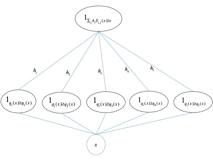
Figure 3: An illustration of a function in ${\cal F}$.

Theorem 14 follows from the next two lemmas (Lemma 16 implies that ${\cal Q}_{\cal F}={\cal Q}_{\mathsf{TV}}$ via Corollary 6).

Lemma 15.

${\cal F}$ has VC dimension at most $10n$.

Lemma 16.

For every $h\geq 0$

$$\min_{v\in{\cal Q}_{\mathsf{TV}}}h\cdot v=\min_{v\in{\cal Q}_{{\cal F}}}h\cdot v$$

Proof of Lemma 15.

We claim that the VC dimension of each ${\cal F}_{i}$ is at most $n$, this will finish the proof by Lemma 13. To see that ${\cal F}_{i}$ has VC dimension at most $n$, we show that its sign-rank (defined below) is at most $n$. This implies the bound on the VC dimension, since the VC dimension is at most the sign-rank (see e.g. (Alon et al., 2016)).

The sign-rank of ${\cal F}_{i}$ is the minimal $d$ such that there is a representation of ${\cal X}$ using $d$-dimensional vectors so that each $f\in{\cal F}_{i}$ corresponds to a $d$-dimensional half-space. Formally, if there is a mapping $\phi:{\cal X}\to{\mathbb{R}}^{d}$ such that for every $f\in{\cal F}_{i}$ there is $u\in{\mathbb{R}}^{d}$ such that $f(x)=1$ if and only if $u\cdot\phi(x)\geq 0$.

To see that the sign-rank of ${\cal F}_{i}$ is at most $n$ consider the mapping

$$\phi(x)=\bigl{(}S_{i,1}(x),\ldots S_{i,i-1}(x),S_{i,i+1}(x),\ldots S_{i,n}(x),1\bigr{)}\in{\mathbb{R}}^{n}.$$

For every $f\in{\cal F}$ with $f={\bf 1}_{\sum_{j\neq i}h_{j}S_{i,j}\geq c}$ pick $v\in{\mathbb{R}}^{n}$ where the first $n-1$ coordinates of $v$ are the $h_{j}$’s for $j\neq i$, and the last coordinate is $-c$. The half-space defined by $u$ indeed corresponds to $f$:

$$f(x)=1\iff{\bf 1}_{\sum_{j\neq i}h_{j}S_{i,j}\geq c}(x)=1\iff\sum_{j\neq i}h_{j}S_{i,j}\geq c\iff v\cdot\phi(x)\geq 0.$$

∎

Proof of Lemma 16.

Lemma 16 follows by a careful inspection of the vertices of ${\cal Q}_{\mathsf{TV}}$. This inspection involves a somewhat technical analysis of the solutions of a related linear program. We provide the proof in Appendix A. ∎

4.1 Proofs of Theorem 8 and Theorem 9

Theorem 8 and Theorem 9 follow from Theorem 10 and Theorem 14, combined with results in Adaptive Data Analysis. We refer the reader to the survey by Dwork et al. (2015) for a detailed introduction.

First, the $O(\frac{n+\log(1/\delta)}{\epsilon^{2}})$ bound in Theorem 8 is a direct corollary of the static algorithm from the previous section (see the discussion prior to Theorem 14’s statement). The second bound in Theorem 8 and the bound in Theorem 9 follows from the two adaptive algorithms $A_{1},A_{2}$ in Theorem 10, as we explain next.

In order for Algorithms $A_{1},A_{2}$ to output a valid distribution $q$, it is required that all of the statistical queries they use are answered with the desired accuracy. Recall that $A_{1}$ uses $2n^{2}/\epsilon$ queries and requires accuracy of $\epsilon/4$ per query and that $A_{2}$ uses $2n\log n/\epsilon$ queries and require accuracy of $\epsilon/2\log n$ per query. To achieve this, one needs to draw enough samples from the target distribution $p$ that suffice for a good-enough estimate. A natural way is to estimate each of the statistical queries by its empirical average. However, since the algorithm is adaptive (i.e. the choice of the statistical query used in iteration $k$ depends on the previous queries and their estimates), this may require a large number of samples from $p$. In particular, there are settings in which if one uses the empirical averages as estimates then $\Omega(k/\epsilon^{2})$ samples are needed in order to answer $k$ adaptive queries adaptively Luckily, the domain of Adaptive Data Analysis has developed clever estimates which achieve significant reductions in the sample complexity. In a nutshell, the idea is to return a noisy version of the empirical averages, and the high-level intuition is that the noise stabilizes this random process and hence makes it more concentrated.

We will use the following results due to Bassily et al. (2016), which improve upon results from Dwork et al. (2015).

Theorem 17 (Infinite domain, Corollay 6.1 in Bassily et al. (2016)).

Let $p$ be the target distribution. Then, there is a mechanism that given $n=n(\epsilon,\delta)$ samples from $p$, answers $k$ adaptive statistical queries such that with probability at least $1-\delta$ each of the provided estimates is $\epsilon$-accurate, and

$$n(\epsilon,\delta)=O\Bigl{(}\frac{\sqrt{k\log\log k}\log^{3/2}(1/\epsilon\delta)}{\epsilon^{2}}\Bigr{)}.$$

Theorem 18 (Finite domain Corollary 6.3 in Bassily et al. (2016)).

Let $p$ be the target distribution. Then, there is a mechanism that given $n=n(\epsilon,\delta)$ samples from $p$, answers $k$ adaptive statistical queries such that with probability at least $1-\delta$ each of the provided estimates is $\epsilon$-accurate, and

$$n(\epsilon,\delta)=O\Bigl{(}\frac{\sqrt{\log\lvert{\cal X}\rvert}\log k\log^{3/2}(1/\epsilon\delta)}{\epsilon^{3}}\Bigr{)}.$$

Algorithm $A_{2}$ combined with Theorem 17 yields the $\tilde{O}(\sqrt{n})$ dependence in Theorem 8, and $A_{1}$ combined with Theorem 18 yields Theorem 9.

5 Lower Bounds

As discussed in the introduction, any finite ${\cal Q}$ can be properly $\alpha=3$-learned by Yatracos’ algorithm. We show that $\alpha=3$ is optimal:

Theorem 19 (Lower bound for infinite domains).

For every $\beta<1$ there is a class ${\cal Q}={\cal Q}(\beta)=\{q_{1},q_{2}\}$ of two densities such that the following holds. Let $A$ be a (possibly randomized) proper learning algorithm for ${\cal Q}$ and let $m$ be a sample complexity bound. Then, there exists a target distribution $p$ such that $\mathsf{opt}=\beta$ and if $A$ gets at most $m$ samples from $p$ as an input then

$$TV(q,p)\geq 3\beta-2\beta^{2}=(3-3\beta)\mathsf{opt}+\beta^{2}\,,$$

with probability at least $\frac{1}{3}$.

The following corollary summarizes that $\alpha=3$ is the threshold for proper learning.

Corollary 20.

For every $\alpha<3$ there exists $\epsilon_{0}>0$ and a class ${\cal Q}$ containing two densities such that no proper algorithm can agnostically learn ${\cal Q}$ with a guarantee of at most

$$\alpha\cdot\mathsf{opt}+\epsilon_{0},$$

and success probability $\delta>2/3$.

Proof.

Let $\alpha<3$. The proof follows from Theorem 19 by plugging $\beta=1-\alpha/3$ , setting $\epsilon_{0}=\beta^{2}$, and noting that $(3-3\beta)\mathsf{opt}+\beta^{2}=\alpha\cdot\mathsf{opt}+\epsilon_{0}$. ∎

For finite domains we get the next version of Theorem 19 which gives a quantitative sample complexity lower bound.

Theorem 21 (Lower bound for finite domains).

Let ${\cal X}$ be a domain of size $N$. Then, for every $\beta<1$ there is a class ${\cal Q}={\cal Q}(\beta)=\{q_{1},q_{2}\}$ of two densities such that the following holds. Let $A$ be a (possibly randomized) proper learning algorithm for ${\cal Q}$. Then, there exists a target distribution $p$ such that $\mathsf{opt}=\beta$ and if $A$ gets at most $\sqrt{N}$ samples from $p$ as an input then

$$TV(q,p)\geq 3\beta-2\beta^{2}=(3-3\beta)\mathsf{opt}+\beta^{2}\,,$$

with probability at least $\frac{1}{3}$.

We will make use of the following lemma which is a simple generalization of Le Cam’s Lemma (see Yu (1997), Lemma 1)

Lemma 22.

Let $\mathcal{D}_{1}$ and $\mathcal{D}_{2}$ be two families of probability distributions, $\mathcal{D}_{i}^{\oplus m}$ denotes the distribution obtained by sampling $p\sim\mathcal{D}_{i}$ (assuming some given fixed distribution over $\mathcal{D}_{i}$) and then drawing $m$ independent samples from $p$. Consider an algorithm (which can be randomized) that determines, given $m$ i.i.d. examples from some $p\in\mathcal{D}_{1}\cup\mathcal{D}_{2}$, whether $p\in\mathcal{D}_{1}$ or $p\in\mathcal{D}_{2}$. Then such an algorithm will have a probability of making a mistake lower bounded by

$$\frac{1}{2}\left(1-\mathsf{TV}(\mathcal{D}_{1}^{\oplus m},\mathcal{D}_{2}^{\oplus m})\right)$$

Proof.

We first assume that the algorithm is deterministic. Any deterministic algorithm deciding whether $p$ comes from $\mathcal{D}_{1}$ or $\mathcal{D}_{2}$ is associated with a set $A\subseteq{\cal X}^{m}$ (the set such that if the sample falls in it, it decides $i=1$, and $i=2$ otherwise). The worst-case probability of the algorithm to err is given by

$$\max\left\lparen\max_{p\in\mathcal{D}_{2}}p^{m}(A),\max_{p\in\mathcal{D}_{1}}p^{m}(\overline{A})\right\rparen$$

which can be lower bounded by the expectation under first choosing between $i=1$ and $i=2$ with probability $1/2$ and then picking $p\sim\mathcal{D}_{i}$:

$$\frac{1}{2}\left(E_{p\sim\mathcal{D}_{1}}p^{m}(A)+E_{p\sim\mathcal{D}_{2}}p^{m}(\overline{A})\right)=\frac{1}{2}\left(1+\mathcal{D}_{1}^{\oplus m}(A)-\mathcal{D}_{2}^{\oplus m}(A)\right)\geq\frac{1}{2}\left(1-\mathsf{TV}(\mathcal{D}_{1}^{\oplus m},\mathcal{D}_{2}^{\oplus m})\right)\,.$$

If the algorithm is randomized then it may pick $A$ randomly, so there is an additional expectation with respect to the distribution over sets $A$ which also leads to the same lower bound. ∎

The following lemma is of independent interest and can be seen as a chain rule for total variation. It essentially says that two distributions are close if there exists an event $E$ with large probability under each of those distributions and such that, conditioned on this event, the two probability distributions are close.

Lemma 23.

Given two probability distributions $P,Q$ on a domain ${\cal X}$ and an event $E\subset{\cal X}$, denoting by $P_{|E}$ and ${\cal Q}_{|E}$ the corresponding conditional distributions (i.e. $P_{|E}(A):=P(A|E)$), we have

$$\mathsf{TV}(P,Q)\leq\mathsf{TV}(P_{|E},Q_{|E})+2P(\overline{E})+2Q(\overline{E})$$

Proof.

$$\mathsf{TV}(P,Q)=\sup_{A}\left|P(A)-Q(A)\right| \leq \sup_{A}\left|P(A\cap E)-Q(A\cap E)\right|+\sup_{A}\left|P(A\cap\overline{E})-Q(A\cap\overline{E})\right|$$

$$\leq \sup_{A}\left|P(E)\left\lparen P(A|E)-Q(A|E)\right\rparen+Q(A|E)\left\lparen P(E)-Q(E)\right\rparen\right|$$

$$+P(\overline{E})+Q(\overline{E})$$

$$\leq P(E)\sup_{A}\left|P(A|E)-Q(A|E)\right|+|P(E)-Q(E)|$$

$$+P(\overline{E})+Q(\overline{E})$$

$$\leq \mathsf{TV}(P_{|E},Q_{|E})+|P(E)-Q(E)|+P(\overline{E})+Q(\overline{E})$$

$$= \mathsf{TV}(P_{|E},Q_{|E})+|P(\overline{E})-Q(\overline{E})|+P(\overline{E})+Q(\overline{E})$$

$$\leq \mathsf{TV}(P_{|E},Q_{|E})+2P(\overline{E})+2Q(\overline{E})$$

∎

Proof of Theorem 19 and Theorem 21.

We first prove Theorem 19 and later note how the proof can be modified to obtain Theorem 21.

Let $\beta<1$ and $m\in\mathbb{N}$; the proof follows by constructing ${\cal Q}=\{q_{1},q_{2}\}$ and two families of distributions $\mathcal{D}_{1},\mathcal{D}_{2}$ with the following properties:

• If $p\in\mathcal{D}_{1}$ then $\mathsf{TV}(q_{1},p)=\beta$ and $\mathsf{TV}(q_{2},p)>3\beta-2\beta^{2}$.

• If $p\in\mathcal{D}_{2}$ then $\mathsf{TV}(q_{2},p)=\beta$ and $\mathsf{TV}(q_{1},p)>3\beta-2\beta^{2}$.

• $\mathsf{TV}(\mathcal{D}_{1}^{\oplus m},\mathcal{D}_{2}^{\oplus m})\leq 1/3$, where $\mathcal{D}_{i}^{\oplus m}$ denotes the distribution obtained by sampling $p$ uniformly from $\mathcal{D}_{i}$ and then taking $m$ independent samples from $p$.

To see how these 3 items conclude the proof of Theorem 19, consider the following game between an adversary and a distinguisher: the adversary randomly picks one of $\mathcal{D}_{1}^{\oplus m},\mathcal{D}_{2}^{\oplus m}$, each with probability $1/2$, and draws a random sample $\vec{x}$ from it. Then, it shows $\vec{x}$ to the distinguisher, whose goal is to determine whether $\vec{x}$ was drawn from $\mathcal{D}_{1}^{\oplus m}$ or from $\mathcal{D}_{2}^{\oplus m}$.

Now, by the first two properties, it follows that any (possibly randomized ) proper learning algorithm for ${\cal Q}$ that uses an input sample of size $m$ and outputs $q_{i}$ such that $\mathsf{TV}(q_{i},p)\leq 3\mathsf{opt}-2\mathsf{opt}^{2}$ with confidence $1-\delta$ can be used by the distinguisher to guarantee a failing probability of at most $\delta$. However, since by Lemma 22 any distinguisher fails with probability at least $1/2-\mathsf{TV}(\mathcal{D}_{1}^{\oplus m},\mathcal{D}_{2}^{\oplus m})/2$, the third property implies that $\delta\geq 1/3$ as required.

Construction of $\mathcal{D}_{1},\mathcal{D}_{2}$.

Set

$$q_{1}(x)=\begin{cases}1-\beta&x\leq 1/2\\ 1+\beta&x>1/2\end{cases},~{}q_{2}(x)=\begin{cases}1+\beta&x\leq 1/2\\ 1-\beta&x>1/2,\end{cases}$$

see Figure 4 for illustration.

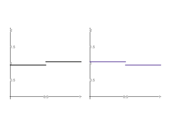
Figure 4: An illustration of $q_{1}$ (left) and $q_{2}$ (right).

In order to define $\mathcal{D}_{1},\mathcal{D}_{2}$, pick a large integer $N=N(m)$ (to be determined later). Partition the unit interval into $2N$ intervals $I_{1},\ldots,I_{2N}$ of size $1/2N$ each. $\mathcal{D}_{1}$ is the family of distributions $p$ of the following form: let $R\subseteq[N]$ be a set of size $k=N\frac{\beta}{2(1+\beta)}$. Set (see Figure 5 for illustration.)

$$p(x)=\begin{cases}1-\beta&x\in I_{j},j\notin R,j\leq N,\\ 2&x\in I_{j},j\in R,j\leq N,\\ 1+\beta&x\in I_{j},j+N\notin R,j>N,\\ 0&x\in I_{j},j+N\in R,j\leq N.\\ \end{cases}$$

$\mathcal{D}_{2}$ is defined analogously as the family of distributions $p$ of the form

$$p(x)=\begin{cases}1+\beta&x\in I_{j},j\notin R,j\leq N,\\ 0&x\in I_{j},j\in R,j\leq N,\\ 1-\beta&x\in I_{j},j+N\notin R,j>N,\\ 2&x\in I_{j},j+N\in R,j\leq N.\\ \end{cases}$$

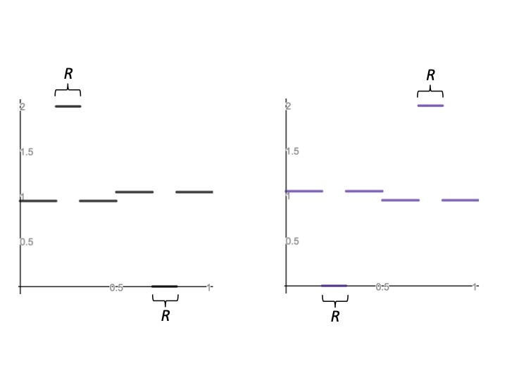
Figure 5: An illustration of a distribution drawn from $\mathcal{D}_{1}$ (left) and of a distribution drawn from $\mathcal{D}_{2}$ (right).

The next claim, which follows from a trivial caclulation, yields the first two items.

Claim 24.

For every $p_{1}\in\mathcal{D}_{1}$:

$$\mathsf{TV}(q_{1},p_{1})=\beta~{}~{}\text{ and }~{}~{}\mathsf{TV}(q_{2},p_{1})=3\beta-\frac{2\beta^{2}}{1+\beta}>3\beta-2\beta^{2}=3(1-\beta)\mathsf{TV}(q_{1},p_{1})+\beta^{2}.$$

Similarly, for every $p_{2}\in\mathcal{D}_{2}$:

$$\mathsf{TV}(q_{2},p_{2})=\beta~{}~{}\text{ and }~{}~{}\mathsf{TV}(q_{1},p_{2})>3(1-\beta)\mathsf{TV}(q_{2},p_{2})+\beta^{2}.$$

The third item follows from the next claim.

Claim 25.

Let $\mathcal{D}\in\{\mathcal{D}_{1}^{\oplus m},\mathcal{D}_{2}^{\oplus m}\}$, and let $E$ denote the event that every interval $I_{j}$ contains at most one sample. Then $\mathcal{D}$ conditioned on $E$ equals to $U^{m}$ conditioned on $E$, where $U^{m}$ denotes the $n$-fold product of the uniform distribution (i.e. $n$ independent samples from the uniform distribution).

This follows since the event $E$ is invariant under any permutation of the intervals $I_{j}$’s and since both $\mathcal{D}_{1},\mathcal{D}_{2}$ are symmetric with respect to the uniform distribution.

The above claim implies that conditioning $\mathcal{D}_{1}^{\oplus m}$ or $\mathcal{D}_{2}^{\oplus m}$ on the event that all samples belong to distinct intervals $I_{j}$ yields the same distribution (hence $\mathsf{TV}({\mathcal{D}_{1}^{\oplus m},}_{|E},{\mathcal{D}_{2}^{\oplus m}}_{|E})=0$). This finishes the proof by noting that the probability of $E$ under both $\mathcal{D}_{1}^{\oplus m}$ and $\mathcal{D}_{2}^{\oplus m}$ is at least

$$\Bigl{(}1-2\cdot\frac{1}{N}\Bigr{)}\cdot\ldots\cdot\Bigl{(}1-2\cdot\frac{m-1}{N}\Bigr{)}\approx\exp(-m^{2}/N),$$

and so picking $N$ sufficiently larger than $m^{2}$ makes this probability arbitrarily close to 1, and in particular at least $11/12$ (setting $N=C\cdot m^{2}$ for some constant $C$ suffices), which, by Lemma 23 gives the upper bound $\mathsf{TV}(\mathcal{D}_{1}^{\oplus m},\mathcal{D}_{2}^{\oplus m})\leq 1/3$.

This finishes the proof of Theorem 19. Theorem 21 follows in a similar manner, by considering the finite domain $\{1,\ldots,2N\}$ and setting

$$q_{1}(x)=\begin{cases}\frac{1-\eta}{2N}&x\leq N\\ \frac{1+\eta}{2N}&x>N\end{cases},~{}q_{2}(x)=\begin{cases}\frac{1+\eta}{2N}&x\leq N\\ \frac{1-\eta}{2N}&x>N,\end{cases}$$

and by identifying each interval $I_{j}$ with $j$.

∎

Appendix A Proof of Lemma 16

Proof.

The desired equality hinges on the Minimax Theorem:

$$\min_{v\in{\cal Q}_{\mathsf{TV}}}h\cdot v=\min_{v\in{\cal Q}_{\mathsf{TV}}}\sum_{i}h_{i}v_{i} =\min_{p\in\Delta({\cal X})}\sum_{i}h_{i}\mathsf{TV}(p,q_{i})$$

$$=\min_{p\in\Delta({\cal X})}\max_{f_{i}:X\to[0,1]}\sum_{i}h_{i}\bigl{(}\mathbb{E}_{p}[f_{i}]-\mathbb{E}_{q_{i}}[f_{i}]\bigr{)}$$

$$=\max_{f_{i}:{\cal X}\to[0,1]}\min_{p\in\Delta({\cal X})}\sum_{i}h_{i}\bigl{(}\mathbb{E}_{p}[f_{i}]-\mathbb{E}_{q_{i}}[f_{i}]\bigr{)}$$ (by the Minimax Theorem von Neumann [1928])

$$=\max_{f_{i}\in\mathsf{conv}({\cal F}_{i})}\min_{p\in\Delta({\cal X})}\sum_{i}h_{i}\bigl{(}\mathbb{E}_{p}[f_{i}]-\mathbb{E}_{q_{i}}[f_{i}]\bigr{)}$$ (this is the technical part that is derived below)

$$=\min_{p\in\Delta({\cal X})}\max_{f_{i}\in\mathsf{conv}({\cal F}_{i})}\sum_{i}h_{i}\bigl{(}\mathbb{E}_{p}[f_{i}]-\mathbb{E}_{q_{i}}[f_{i}]\bigr{)}$$ (by the Minimax Theorem)

$$=\min_{p\in\Delta({\cal X})}\max_{f_{i}\in{\cal F}_{i}}\sum_{i}h_{i}\bigl{(}\mathbb{E}_{p}[f_{i}]-\mathbb{E}_{q_{i}}[f_{i}]\bigr{)}$$ (a linear function over a convex set is maximized at a vertex)

$$=\min_{p\in\Delta({\cal X})}\sum_{i}h_{i}d_{{\cal F}_{i}}(p,q_{i})\leq h_{i}d_{{\cal F}}(p,q_{i})=\min_{v\in{\cal Q}_{{\cal F}}}h\cdot v.$$

We next turn to prove the main inequality:

$$\max_{f_{i}:{\cal X}\to[0,1]}\min_{p\in\Delta({\cal X})}\sum_{i}h_{i}\bigl{(}\mathbb{E}_{p}[f_{i}]-\mathbb{E}_{q_{i}}[f_{i}]\bigr{)}=\max_{f_{i}\in\mathsf{conv}({\cal F}_{i})}\min_{p\in\Delta({\cal X})}\sum_{i}h_{i}\bigl{(}\mathbb{E}_{p}[f_{i}]-\mathbb{E}_{q_{i}}[f_{i}]\bigr{)}.$$

First, note that the direction “$\geq$” is trivial since in the left-hand-side the maximum is not restricted to $f_{i}\in\mathsf{conv}(F)$. The other direction follows by analyzing the $f_{i}$’s that maximize the program

$$\max_{f_{i}:{\cal X}\to[0,1]}\min_{p\in\Delta({\cal X})}\sum_{i}h_{i}\bigl{(}\mathbb{E}_{p}[f_{i}]-\mathbb{E}_{q_{i}}[f_{i}]\bigr{)}.$$ (5)

Let us first write the objective $T(f_{i})=T(f_{1},\ldots,f_{n}):=\min_{p\in\Delta({\cal X})}\sum_{i}h_{i}(\mathbb{E}_{p}[f_{i}]-\mathbb{E}_{q_{i}}[f_{i}])$ more explicitly:

$$T(f_{i}) =\min_{p\in\Delta({\cal X})}\sum_{i}h_{i}\bigl{(}\mathbb{E}_{p}[f_{i}]-\mathbb{E}_{q_{i}}[f_{i}]\bigr{)}$$

$$=\min_{p\in\Delta({\cal X})}\Bigl{(}\sum_{x}p(x)\sum_{i}h_{i}f_{i}(x)-\sum_{x}\sum_{i}q_{i}(x)h_{i}f_{i}(x)\Bigr{)}$$

$$=\min_{p\in\Delta({\cal X})}\Bigl{(}\sum_{x}p(x)\sum_{i}h_{i}f_{i}(x)\Bigr{)}-\sum_{x}\sum_{i}q_{i}(x)h_{i}f_{i}(x).$$

We want to show that there exists a maximizer $f_{i}^{*}$ of $T(f_{i})$ such that $f_{i}^{*}\in\mathsf{conv}({\cal F}_{i})$. To see this, it will be more convenient to express $T(f_{i})$ in the following maximization form:

Claim 26.

For every choice of the $f_{i}$’s the function $T(f_{i})$ equals to the value of the following linear program in the variable $\lambda\in{\mathbb{R}}$:

$$\max_{\lambda}~{}~{}~{}\lambda-\sum_{x}\sum_{i}h_{i}f_{i}(x)q_{i}(x)$$

$$\text{subject to}~{}~{}~{}\lambda\leq\sum_{i}h_{i}f_{i}(x),~{}~{}~{}\forall x\in{\cal X}.$$

Proof.

We show that both $T(f_{i})$ and the value of the above program are equal to

$$\min_{x}\bigl{(}h_{i}f_{i}(x)\bigr{)}-\sum_{x}\sum_{i}h_{i}f_{i}(x)q_{i}(x).$$

Indeed, for the linear program it follows directly from its definition.

To derive it also for $T(f_{i})$, recall that we already established that

$$T(f_{i})=\min_{p\in\Delta({\cal X})}\Bigl{(}\sum_{x}p(x)\sum_{i}h_{i}f_{i}(x)\Bigr{)}-\sum_{x}\sum_{i}q_{i}(x)h_{i}f_{i}(x),$$

Thus, its value is obtained by distributions $p^{*}$ that minimize $\sum_{x}p(x)\sum_{i}h_{i}f_{i}(x)$. Clearly, $p^{*}$ minimizes this sum if it concentrates all its weight on the $x$’s that minimizes $\sum_{i}h_{i}f_{i}(x)$, and therefore $T(f_{i})=\min_{x}h_{i}f_{i}(x)-\sum_{x}\sum_{i}q_{i}(x)h_{i}f_{i}(x)$, as required. ∎

By Claim 26 it suffices to show that there are $f_{i}^{*}\in\mathsf{conv}({\cal F})$ that maximize the following linear program

$$\max_{f_{i},\lambda}~{}~{}~{}\lambda-\sum_{x}\sum_{i}q_{i}(x)h_{i}f_{i}(x)$$ (6)

$$\text{subject to}~{}~{}~{}\lambda\leq\sum_{i}h_{i}f_{i}(x),~{}~{}~{}\forall x\in{\cal X}$$

$$\text{and to}~{}~{}~{}f_{i}:{\cal X}\to[0,1],~{}~{}~{}\forall i\leq n.$$

Note that since the maximization is over both $\lambda$ and the $f_{i}$’s then we can first maximize over the $f_{i}$’s (keeping $\lambda$ fixed), and then optimize over $\lambda$. In other words, it suffices to show that for a fixed $\lambda$, the optimal $f_{i}$’s satisfy $f_{i}\in\mathsf{conv}({\cal F}_{i})$. Since $\lambda$ is fixed, we can consider the simpler objective of

$$\min_{f_{i}}~{}~{}~{}\sum_{x}\sum_{i}q_{i}(x)h_{i}f_{i}(x).$$

Since the constraints over different $x$’s are independent, we can optimize each $f_{i}(x)$ point-wise by solving:

$$\min_{f_{i}}~{}~{}~{}\sum_{i}q_{i}(x)h_{i}f_{i}(x)$$

$$\text{subject to}~{}~{}~{}\sum_{i}h_{i}f_{i}(x)\geq\lambda,$$

$$\text{and to}~{}~{}~{}f_{i}(x)\in[0,1],~{}~{}~{}\forall i\leq n.$$

The latter form is easier to handle: Sort the $q_{i}(x)$ according to their values; for simplicity and without loss of generality assume that $q_{1}(x)\leq q_{2}(x)\leq\ldots q_{n}(x)$. We claim that an optimal solution can be obtained by traversing the $i$ from $1$ to $n$, and setting the corresponding $f_{i}$ to as large as possible until feasibility is achieved (i.e. until $\sum_{i}h_{i}f_{i}(x)=\lambda$). More formally, the following solution is optimal:

$$f_{i}(x)=\begin{cases}1&\sum_{j\leq i}h_{j}<\lambda,\\ \frac{\lambda-\sum_{j<i}h_{j}}{h_{i}}&\sum_{j<i}h_{j}<\lambda\text{ and }\sum_{j<i}h_{j}+h_{i}\geq\lambda,\\ 0&\text{otherwise.}\end{cases}$$

Indeed, else there would be some $i$ with $\sum_{j<i}h_{j}>\lambda$ for which $q_{i}(x)>0$, and we could decrease $f_{i}(x)$ to $0$ and increase $f_{j}(x)$ for for some $j$’s with $j<i$, which could only improve (decrease) the objective.

The proof is finished by noticing that

$$f_{i}(x)=1_{\sum_{j\neq i}h_{j}A_{i,j}(x)<\lambda}~{}~{}~{}~{}\text{ or }~{}~{}~{}~{}f_{i}(x)=t\cdot 1_{\sum_{j\neq i}h_{j}A_{i,j}(x)<\lambda},$$

for $t=\frac{\lambda-\sum_{j<i}h_{j}}{h_{i}}\leq 1$, and in either way $f_{i}\in\mathsf{conv}({\cal F}_{i})$ (note that indeed $t\cdot 1_{\sum_{j}h_{j}A_{i,j}(x)\leq\lambda^{*}}$ is in $\mathsf{conv}({\cal F}_{i})$ since it is a convex combination of $1_{\sum_{j}h_{j}A_{i,j}(x)\leq\lambda^{*}}$ and the all-zeros function, which are both in ${\cal F}_{i}$).

∎

References

- Alon et al. [2016] N. Alon, S. Moran, and A. Yehudayoff. Sign rank versus VC dimension. In V. Feldman, A. Rakhlin, and O. Shamir, editors, Proceedings of the 29th Conference on Learning Theory, COLT 2016, New York, USA, June 23-26, 2016, volume 49 of JMLR Workshop and Conference Proceedings, pages 47–80. JMLR.org, 2016.
- Ashtiani et al. [2018a] H. Ashtiani, S. Ben-David, N. Harvey, C. Liaw, A. Mehrabian, and Y. Plan. Nearly tight sample complexity bounds for learning mixtures of gaussians via sample compression schemes. In S. Bengio, H. Wallach, H. Larochelle, K. Grauman, N. Cesa-Bianchi, and R. Garnett, editors, Advances in Neural Information Processing Systems 31, pages 3416–3425. Curran Associates, Inc., 2018a.
- Ashtiani et al. [2018b] H. Ashtiani, S. Ben-David, and A. Mehrabian. Sample-efficient learning of mixtures. In Proceedings of the Thirty-Second AAAI Conference on Artificial Intelligence, (AAAI-18), the 30th innovative Applications of Artificial Intelligence (IAAI-18), and the 8th AAAI Symposium on Educational Advances in Artificial Intelligence (EAAI-18), New Orleans, Louisiana, USA, February 2-7, 2018, pages 2679–2686, 2018b.
- Bassily et al. [2016] R. Bassily, K. Nissim, A. Smith, T. Steinke, U. Stemmer, and J. Ullman. Algorithmic stability for adaptive data analysis. In Proceedings of the Forty-eighth Annual ACM Symposium on Theory of Computing, STOC ’16, pages 1046–1059, New York, NY, USA, 2016. ACM. ISBN 978-1-4503-4132-5. doi: 10.1145/2897518.2897566.
- Chan et al. [2014] S. Chan, I. Diakonikolas, R. A. Servedio, and X. Sun. Near-optimal density estimation in near-linear time using variable-width histograms. In NIPS, pages 1844–1852, 2014.
- Daniely and Shalev-Shwartz [2014] A. Daniely and S. Shalev-Shwartz. Optimal learners for multiclass problems. In M. Balcan, V. Feldman, and C. Szepesvári, editors, Proceedings of The 27th Conference on Learning Theory, COLT 2014, Barcelona, Spain, June 13-15, 2014, volume 35 of JMLR Workshop and Conference Proceedings, pages 287–316. JMLR.org, 2014.
- Devroye and Gyorfi [1985] L. Devroye and L. Gyorfi. Nonparametric Density Estimation: The L1 View. Wiley Interscience Series in Discrete Mathematics. Wiley, 1985. ISBN 9780471816461.
- Devroye and Lugosi [2001] L. Devroye and G. Lugosi. Combinatorial methods in density estimation. Springer, 2001.
- Devroye and Lugosi [2004] L. Devroye and G. Lugosi. Bin width selection in multivariate histograms by the combinatorial method. Test, 13(1):129–145, Jun 2004. ISSN 1863-8260. doi: 10.1007/BF02603004.
- Diakonikolas [2016] I. Diakonikolas. Learning structured distributions. In Handbook of Big Data, pages 267–283. Chapman and Hall/CRC, 2016.
- Diakonikolas et al. [2017] I. Diakonikolas, D. M. Kane, and A. Stewart. Statistical query lower bounds for robust estimation of high-dimensional gaussians and gaussian mixtures. In FOCS, pages 73–84. IEEE Computer Society, 2017.
- Diakonikolas et al. [2018a] I. Diakonikolas, D. M. Kane, and A. Stewart. List-decodable robust mean estimation and learning mixtures of spherical gaussians. In STOC, pages 1047–1060. ACM, 2018a.
- Diakonikolas et al. [2018b] I. Diakonikolas, J. Li, and L. Schmidt. Fast and sample near-optimal algorithms for learning multidimensional histograms. In S. Bubeck, V. Perchet, and P. Rigollet, editors, Proceedings of the 31st Conference On Learning Theory, volume 75 of Proceedings of Machine Learning Research, pages 819–842. PMLR, 06–09 Jul 2018b.
- Dwork et al. [2015] C. Dwork, V. Feldman, M. Hardt, T. Pitassi, O. Reingold, and A. Roth. The reusable holdout: Preserving validity in adaptive data analysis. Science, 349(6248):636–638, 2015. ISSN 0036-8075. doi: 10.1126/science.aaa9375.
- Jiao et al. [2018] J. Jiao, Y. Han, and T. Weissman. Minimax estimation of the distance. IEEE Transactions on Information Theory, 64(10):6672–6706, Oct 2018. ISSN 0018-9448. doi: 10.1109/TIT.2018.2846245.
- Kalai et al. [2012] A. T. Kalai, A. Moitra, and G. Valiant. Disentangling gaussians. Commun. ACM, 55(2):113–120, 2012. doi: 10.1145/2076450.2076474.
- Kothari et al. [2018] P. K. Kothari, J. Steinhardt, and D. Steurer. Robust moment estimation and improved clustering via sum of squares. In Proceedings of the 50th Annual ACM SIGACT Symposium on Theory of Computing, STOC 2018, Los Angeles, CA, USA, June 25-29, 2018, pages 1035–1046, 2018. doi: 10.1145/3188745.3188970.
- Lugosi and Nobel [1996] G. Lugosi and A. Nobel. Consistency of data-driven histogram methods for density estimation and classification. Ann. Statist., 24(2):687–706, 04 1996. doi: 10.1214/aos/1032894460.