Space-Time Discriminant to Separate Double-Beta Decay from ⁸B Solar Neutrinos in Liquid Scintillator

Abstract

We present a technique for separating nuclear double beta-decay events from background ⁸B solar neutrino interactions in a liquid scintillator detector instrumented with photo-detectors with mm space and 100-psec time resolutions. The technique uses position and time information of detected photo-electrons (PEs) to separate directional Cherenkov light from isotropic scintillation light in the reconstruction of the kinematics of candidate events. Here we introduce a Cherenkov-scintillation space time boundary defined as the light cone in the 2-dimensional space of the arrival time and the polar angle of each PE with respect to the axis from the center of the detector to the vertex. The PEs located near the boundary correspond to photons that were emitted early and contain a high fraction of directional Cherenkov PEs. We apply weights derived from the distance to the boundary of each individual PE, which are then used in a spherical harmonics analysis that separates the two-track event topology of double-beta decay from the one-track topology of ⁸B events. The Geant-4 simulation assumes a detector of 6.5 m radius filled with ¹³⁰Te-loaded liquid scintillator and surrounded by photo-detectors with time and space resolutions of 100 ps and 3 mm respectively. The scintillation properties and photo-detector quantum efficiency are modeled after KamLAND. Assuming a fiducial volume of 3 m radius, a photo-coverage of 65% and vertex resolution of $\sigma_{r_{v}}=$ 5.2 cm at 2.53 MeV the method of reconstructing event topology predicts factors of 1.3 and 2.3 in background suppression at 90% and 70% signal efficiency respectively. Additionally, the PEs near the Cherenkov-scintillation space-time boundary can be used to reconstruct the directionality of one-electron candidate events, allowing for further ⁸B background suppression due to the correlation between the direction of the scattered electron and the position of the sun. We find polar and azimuthal angular resolutions of 0.46 and 0.84 radians respectively. We show the dependence of the topology and directionality reconstructions on photo-coverage and vertex resolution, and discuss directions in detector development that can improve background suppression; however determination of a combined background rejection factor based on topological and directional reconstruction is a subject of further studies using a detailed detector-specific background model.

1 Introduction

Today it is still not known whether for a given helicity the neutrino mass eigenstates are identical to the corresponding eigenstates of the anti-neutrino, i.e. whether the neutrino is a Majorana particle [1].

Searching for neutrinoless double-beta decay ($0\nu\beta\beta$-decay) [2] is the most feasible experimental technique to determine if the neutrino is a Majorana particle. Contrary to two-neutrino double-beta decay [3], neutrinoless double-beta decay, $(Z,A)\rightarrow(Z+2,A)+2e^{-}$, violates electron lepton number by two units and therefore has a potential to probe physics beyond the Standard Model [4]. At the same time, according to the Schechter-Valle theorem [5], the observation of $0\nu\beta\beta$-decay would guarantee the existence of a non-zero Majorana mass term for the neutrino.

To explore $0\nu\beta\beta$-decay beyond the current experimental lower limits on half-life of up to $\sim$$10^{26}$ years [7, 8, 9, 10], all currently planned $0\nu\beta\beta$-decay experiments aim for a ton-scale active isotope mass [11]. There are several detector technologies capable of reaching a sensitivity to a $0\nu\beta\beta$-decay half-life of $10^{27}$-$10^{28}$  years by instrumenting several tons of isotope [12, 13, 14]. Probing Majorana masses in the regime of the non-degenerate normal neutrino mass hierarchy may require a detector with an active isotope mass approaching a kilo-ton [15].

The scalability, self-shielding, and good energy resolution of liquid scintillator detectors makes them a competitive option for the search for $0\nu\beta\beta$-decay [8]. The use of Cherenkov light in a liquid scintillator detector can enhance the event identification capabilities of liquid scintillator detectors. Cherenkov light has been successfully used for event reconstruction in a diluted liquid scintillator in the LSND experiment [16]. However, the light yield of the diluted scintillator of LSND would not be sufficient to achieve the energy resolution required for $0\nu\beta\beta$-decay searches. In addition, LSND was looking for electron tracks with energy of about 45 MeV. This is to be compared with the $\sim$1-2 MeV electrons from a $0\nu\beta\beta$-decay. Reconstruction of events with energies down to 3-5 MeV using Cherenkov light in pure water has been done at the Super-Kamiokande experiment [17, 18]. In this work we focus on the reconstruction of $0\nu\beta\beta$-decay events in a high light-yield liquid scintillator.

To our knowledge, the idea of using Cherenkov light in searches for $0\nu\beta\beta$-decay was first discussed in Ref. [19]. Development of a scintillator with a long time constant to extract directional information from Cherenkov light in $0\nu\beta\beta$-decay searches has been suggested in Ref. [15]. The first feasibility studies of using Cherenkov light in a regular liquid scintillator with the scintillation light yield sufficient for $0\nu\beta\beta$-decay search were done in Ref. [20]. It was shown that by correlating PE position and time measurements using fast photo-detectors with time resolution of $\sim$100 ps one can reconstruct the direction of electrons in the energy range between 1.4 and 5 MeV. This in turn, opens a possibility to suppress backgrounds in $0\nu\beta\beta$-decay searches, including background from ⁸B solar neutrinos.

In a kilo-ton liquid scintillator detector, the electrons from elastic scattering of ⁸B solar neutrinos can become a dominant background [21]. A path towards suppression of ⁸B background has been shown in previous work [20, 22]. The background suppression relies on separation of directional Cherenkov light from the abundant isotropic scintillation light using fast photo-detectors. Cherenkov photons then allow reconstruction of the event topology, which is different for the two-electron $0\nu\beta\beta$-decay signal and for one-electron ⁸B background events [22]. Whenever the $0\nu\beta\beta$-decay signal events have only one electron above Cherenkov threshold or have two electrons emitted at a very small angle, the ⁸B background can be suppressed by reconstructing the direction of the electron(s), which in the case of ⁸B events correlates with the position of the sun [15, 23].

Separation of Cherenkov light from scintillation light has been demonstrated in various experimental settings [16, 24, 25, 26] including detection of Cherenkov light from 1-2 MeV electrons in linear alkylbenzene [27]. Currently, research towards an effective separation of Cherenkov light from scintillation light is being actively pursued [28, 29, 30, 31, 32, 33, 34, 35]. For example, the ANNIE experiment [36] plans to fill their detector volume with a water-based liquid scintillator [37, 38] to explore a hybrid event reconstruction scheme that uses Cherenkov and scintillation light for events with energy around 1 GeV [39]. The NuDot experiment aims to demonstrate kinematics reconstruction in a one-ton liquid scintillator detector for events in the energy range relevant for $0\nu\beta\beta$-decay [27].

New techniques have been developed for event reconstruction in liquid scintillator detectors to complement calorimetric measurements [40, 41, 42] including those targeting separation of $0\nu\beta\beta$-decay from cosmic muon spallation background [43].

Here we present new developments in the reconstruction of the $0\nu\beta\beta$-decay event topology and in measuring electron directionality for ⁸B background suppression. Continuing the work described in Ref. [22] we use spherical functions to construct topology-dependent rotation invariants. For directionality reconstruction, similarly to Ref. [20], we also use the “center of gravity” of a photo-electron (PE) sample with an enhanced fraction of Cherenkov light. However, the technique presented here is an improvement over Refs. [20, 22] in the following areas.

First, instead of applying a fixed time cut in the case of central events [20] or a pre-defined ad-hoc time window in the case of events uniformly distributed throughout the entire fiducial volume [22] to separate Cherenkov and scintillation light, we identify a Cherenkov-scintillation space-time boundary with a general expression as the light cone in the 2-dimensional plane of the arrival time and the polar angle with respect to the axis from the center of the detector to the vertex, which allows selecting a PE sample with an increased fraction of Cherekov PEs. In this paper, the time displacement of each PE from the Cherenkov-scintillation space time boundary is used to assign higher weights to Cherenkov PEs.

Second, we construct the spherical harmonics power spectrum, called here the S-spectrum, using a summation over each individual PE instead of integrating over $\Delta\theta\times\Delta\phi$ segments, which in Ref.[22] on average have a solid angle of $\sim$0.063 corresponding to the surface area of 2.65 m² for a 6.5m radius sphere. This allows for the efficient use of spatial information of photo-electrons. At the same time this improves the CPU time needed to process one event compared to the technique in Ref.[22], because there is no numerical integration involved in the calculation of the S-spectrum in the new method.

Third, while the reconstruction of electron directionality has been demonstrated in Ref. [20] for the case of central events, here we demonstrate electron directionality reconstruction for all events uniformly distributed throughout the fiducial volume of the detector.

Finally, we use a maximum likelihood method to quantify the background suppression that can be obtained from two different variables derived from the S-spectrum. This is a step towards a multi-variative analysis to extract more information from the S-spectrum and to account for additional correlations between the S-spectrum components and other attributes of $0\nu\beta\beta$-decay candidate events such as the position of the vertex, and the angle and the energy split between the electrons.

While we targeted the ⁸B solar neutrino background suppression, the topological reconstruction is also applicable for the suppression of backgrounds due to one-track single-beta decays. The directionality reconstruction can be instrumental for studying CNO-cycle solar neutrinos [44] and geo-neutrinos [45].

The organization of the paper is as follows. Section 2 describes the detector model and event simulation details. The Cherenkov-scintillation space-time boundary is introduced in Section 3. Section 4 describes ⁸B background suppression based on event topology reconstruction. Section 5 describes directionality reconstruction. Conclusions are summarized in Section 6.

2 Detector Model and Event Simulation

We use the same Geant-4 based simulation described in Refs. [20, 22]. The detector is a sphere with a radius of 6.5 m filled with liquid scintillator. The scintillator composition has been chosen to match a KamLAND-like scintillator [46], which consists of 80% n-dodecane, 20% pseudocumene and 1.52 g/l PPO with a density of $\rho$ = 0.78 g/ml. However, we deviate from the baseline KamLAND case in that the re-emission of absorbed photons in the scintillator bulk volume and optical scattering, specifically Rayleigh scattering, have not yet been included. A test simulation shows that the effect of optical scattering is negligible [20].

The inner sphere surface is used as the photo-detector. It is treated as fully absorbing with no reflections. We consider photo-cathode coverage ranging from 10% to 100% with 65% being our default coverage choice. We distribute 7682 identical spherical caps over the detector sphere and insert inside identical circular photo-detectors. We vary the radii of the photo-detectors from 47 mm to 120 mm to achieve a desired photo-coverage.

The assumed quantum efficiency (QE) is that of a typical bialkali photo-cathode (Hamamatsu R7081 PMT [47], see also Ref. [48]), which is 12% for Cherenkov light and 23% for scintillation light. We assume a photo-detector transit-time-spread (TTS) of 100 ps, and PE position resolution of 3 mm in both of the two dimensions, which, for example, are well within demonstrated performance of large-area picosecond photo-detectors (LAPPD) [49, 50]. We neglect the threshold effects in the photo-detector readout electronics, noise effects, and contributions to time resolution other than the photo-detector TTS.

We define the fiducial volume as a sphere of 3 m radius and simulate signal and background events uniformly distributed within that fiducial volume. Following the same strategy as in Ref. [22] we smear the vertex along $x$, $y$, and $z$ directions with three independent Gaussian distributions of the same width, $\sigma_{x}=\sigma_{y}=\sigma_{z}=$ 3 cm. This vertex smearing introduces an uncertainty on the vertex position of $\sigma_{r_{v}}=$ 5.2 cm, which is based on an earlier study of vertex reconstruction [20]. The vertex position, $r_{v}$, is then treated as a reconstructed vertex position.

The details of the event simulation and discussion on kinematics of ¹³⁰Te $0\nu\beta\beta$-decay and ⁸B events can be found in Ref. [22]. We simulate the kinematics of 0$\nu\beta\beta$-decay events using a custom Monte Carlo with momentum and angle-dependent phase space factors for 0$\nu\beta\beta$-decay [51]. Electrons from elastic scattering of ⁸B solar neutrinos have a nearly flat energy spectrum around the ¹³⁰Te $0\nu\beta\beta$-decay Q-value of 2.53 MeV[52]. We simulate ⁸B background as a single monochromatic electron with energy of 2.53 MeV.

3 Cherenkov-Scintillation Space-Time Boundary

For any given sufficiently small area on the detector surface that is hit by the Cherenkov light, the majority of the scintillation PEs arrive after the Cherenkov PEs regardless of the vertex position and the event type. In the 2-dimensional plane of the arrival time and the polar angle with respect to the axis from the center of the detector to the vertex, the Cherenkov-scintillation space-time boundary $t_{c}(\theta)$ is defined to be the light cone with a certain speed of light:

$$t_{c}(\theta)=\frac{\sqrt{R^{2}+r_{v}^{2}-2Rr_{v}\cos\theta}}{c(n)}-\frac{R-r_{v}}{c(n)},$$ (1)

where $R$ is the radius of the detector’s inner sphere, $r_{v}$ is the length of the vertex displacement vector $\vec{r}_{v}$ from the center of the sphere, $\theta$ is the angle between the vertex displacement vector $\vec{r}_{v}$ and the photon hit vector from the center of the sphere, and $c(n)$ is the speed of the scintillation light in the liquid scintillator. We use an average value for the index of refraction of $n=$ 1.53 to determine $c(n)$. The majority of scintillation PEs have arrival times, $t_{sci}(\theta)$, exceeding $t_{c}(\theta)$, $t_{sci}(\theta)>t_{c}(\theta)$.

The first term in Eq.1 corresponds to an estimate of the time for the first scintillation PE emitted at angle $\theta$ to reach the detector sphere. The second term is an estimate of the travel time for the earliest scintillation PEs, i.e. the scintillation PE emitted at $\theta=0$, along the vertex displacement vector $\vec{r}_{v}$.

Figure 1 shows the arrival time of PEs, $t_{PE}$, relative to the very first PE as a function of the polar angle in one $0\nu\beta\beta$-decay event and one ⁸B event. One can see that all the Cherenkov PEs are located near the scintillation PE boundary. In the example $0\nu\beta\beta$-decay signal event shown in Fig. 1, the vertex displacement from the center is $r_{v}$ = 229 cm and the vertex displacement in the ⁸B background event is $r_{v}$ = 292 cm.

We define the PEs time displacement, $t_{d}(t_{PE},\theta)$, from the Cherenkov-scintillation space-time boundary as

$$t_{d}(t_{PE},\theta)=t_{PE}-t_{c}(\theta).$$ (2)

The distributions of the time displacement of all PEs at all polar angles in 10,000 signal and 10,000 background events are also shown in Fig. 1. The PE time displacement can be used to select a sample of PEs with higher fraction of Cherenkov PEs compared to a full sample of all PEs in the event.

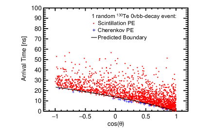
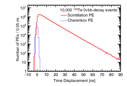
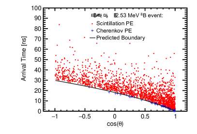
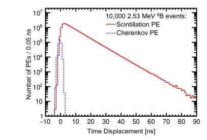
Figure 1: [Left]: The space-time boundaries $t_{c}(\theta)$ (solid black line) between Cherenkov PEs (blue crosses) and scintillation PEs (red dots) for one $0\nu\beta\beta$-decay signal event (top left) and one ⁸B background event (bottom left). The z-axis is chosen to be aligned with the vertex displacement vector $r_{v}$ from the center of the detector sphere; $\theta$ is defined to be the angle between the z-axis and the photon hit vector $\vec{r}_{i}$ from the center of the detector sphere. The arrival time $t$ is defined relative to the earliest PE detection. [Right]: Distributions of the time displacement $t_{d}$ of Cherenkov PEs (dotted blue line) and scintillation PEs (solid red line) from the space-time boundary $t_{c}(\theta)$, $t_{d}(t_{PE},\theta)=t_{PE}-t_{c}(\theta)$, for 10,000 $0\nu\beta\beta$-decay signal events (top right) and 10,000 ⁸B background (bottom right) events. The majority of the scintillation PEs (solid red line) have a larger time displacement $t_{d}$. All Cherenkov PEs (dotted blue line) are located near the boundary.

The deviations from the prediction of the Cherenkov-scintillation space-time boundary given by Eq. 1 arise due to the uncertainty on the location of the vertex, not knowing the group velocity of individual photons, and not knowing a priori whether the earliest PE is Cherenkov or scintillation.

In the subsequent analysis, we assign a weight $W(t_{PE},\theta)$ to each individual PE based on the time displacement $t_{d}(t_{PE},\theta)$ in order to increase the contribution from directional Cherenkov light, and to eliminate the effect of the time translation uncertainty of the space-time boundary due to not knowing the type of the earliest PE. In particular, the weight $W(t,\theta)$ is designed such that the total weight on the Cherenkov PEs relative to the scintillation PEs is independent of the time translation uncertainty. We define the weight as

$$W(t_{PE},\theta)=\exp\left[-\frac{t_{d}(t_{PE},\theta)}{\tau}\right],$$ (3)

where $\tau$ is a time constant optimized to be 0.4 ns. The chosen value of $\tau=$ 0.4 ns suppresses the contribution of scintillation PEs while still preserves a sufficient contribution from all Cherenkov PEs.

4 Event Topology Reconstruction

4.1 Rotationally Invariant S-spectrum

Using the angular coordinates of PEs we construct the following rotationally invariant series, dubbed the ‘S-spectrum’:

$$S_{\ell}=\frac{\sum_{m=-\ell}^{\ell}\absolutevalue{\sum_{i=1}^{N_{PE}}W(t_{i},\theta_{i})Y_{\ell m}(\theta_{i},\phi_{i})}^{2}}{\absolutevalue{\sum_{i=1}^{N_{PE}}W(t_{i},\theta_{i})}^{2}},$$ (4)

where $N_{PE}$ is the total number of PEs, $\theta_{i}$ and $\phi_{i}$ are the spherical coordinates of each PE and $Y_{\ell m}(\theta,\phi)$ are the tesseral harmonics. See B for a detailed discussion on the S-spectrum normalization and rotation invariance.

We note that S-spectrum computation time scales linearly with the number of PE hits, $N_{PE}$. In comparison, the computation time of the fast Fourier transform and spherical Fourier transform algorithms on a grid with $N$ points scale as $N\times Log(N)$ [53, 54, 55].

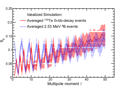
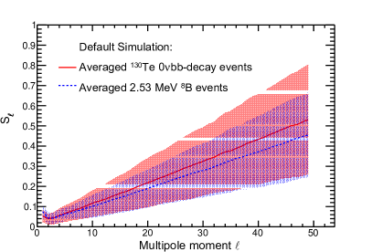
Figure 2: The S-spectrum averaged over 100 (left) or 1000 (right) $0\nu\beta\beta$-decay signal (solid red line) and ⁸B background (dotted blue line) events. Shaded areas show one standard deviation from the mean value indicating a typical event-by-event $S_{\ell}$ spread at each $\ell$. [Left]: Simulation of 100 events using idealized simulation settings: events originated at the center of the detector sphere, photo-coverage is 100%, QE is 30% for both scintillation and Cherenkov light, multiple scattering turned off. To increase the contribution from Cherenkov PEs relative to scintillation PEs, only PEs that arrive within 1.5 ns after the first PE in each event are used for S-spectrum calculations. The signal S-spectrum has smaller $S_{1}$, larger slope $\alpha$, and a more rapid oscillation pattern in the S-spectrum compared to the background S-spectrum. [Right]: Simulation of 1000 events using default simulation settings: events uniformly distributed throughout the fiducial volume of R$<$3 m, photo-coverage is 60%, QE is 23% for scintillation light and 12% for Cherenkov light, multiple scattering is properly included in the simulation. To increase the contribution from Cherenkov PEs relative to scintillation PEs, each PE is assigned weight $W(t_{d},\theta)$ according to Eq. 3. The signal S-spectrum has smaller $S_{1}$ and larger slope $\alpha$ compared to the background S-spectrum.

The S-spectrum series, $S_{\ell}$, is determined by the PE distribution over the sphere and therefore can be used to distinguish different event topologies. Figure 2 shows the S-spectrum averaged over multiple $0\nu\beta\beta$-decay signal and ⁸B background events for idealized (Fig. 2, left) and realistic (Fig. 2, right) simulations.

In the idealized simulation, events are simulated only at the center of the detector, multiple scattering is turned off, photo-coverage is 100%, and the QE is 30% for all photons regardless of the wavelength. Comparing with the background the signal S-spectrum has smaller $S_{1}$, larger overall slope $\alpha$, and a more rapid oscillation pattern.

The S-spectrum shape dependence on the photon distribution is discussed in the appendices of Ref. [56]. For example, on average, the Cherenkov PE distribution is more symmetric in the case of the two-track 0$\nu\beta\beta$ signal than the one-track ⁸B background, leading to smaller $S_{1}$ values for the signal.

The idealized simulation is shown here for illustration purposes only. Unless noted otherwise, in this paper we use the default simulation settings as described in Sec. 2. In the default simulation, multiple scattering is included, photo-coverage is 65%, QE is of a typical bialkali photo-cathode, and all simulated events are uniformly distributed in the detector fiducial volume of R$<$3 m.

As shown in Fig. 2 (right) for events simulated with the default simulation settings the main differences between signal and background S-spectra are in the values of $S_{1}$ and the slope $\alpha$. Therefore we use the $S_{1}$ and $\alpha$ parameters to separate $0\nu\beta\beta$-decay signal from ⁸B background events.

The distribution of $S_{1}$ and $\alpha$ parameters for $0\nu\beta\beta$-decay signal and ⁸B background events are shown in Fig. 3. Using these two distributions we construct a likelihood function to separate signal and background events.

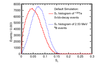
Figure 3: [Left]: Comparison of the $S_{1}$ parameter between 200,000 simulated 0$\nu\beta\beta$ signal (solid red line) and ⁸B background (dotted blue line) events. The default simulation settings are used. [Right]: Comparison of the $\alpha$ parameter between 200,000 0$\nu\beta\beta$ signal (solid red line) and ⁸B background (dotted blue line) events.

4.2 Maximum Likelihood Estimation

For a candidate event in the fiducial volume, the values of parameters $S_{1}$ and $\alpha$ constitute a measurement, $\vec{S}_{meas}=(S_{1},\alpha)$. The likelihood, $p(2e|\vec{S}_{meas})$, for such an event to be a 0$\nu\beta\beta$-decay signal is given by:

$$p(2e|\vec{S}_{meas})=\frac{p(\vec{S}_{meas}|2e)}{p(\vec{S}_{meas}|1e)+p(\vec{S}_{meas}|2e)}=\frac{p(S_{1}|2e)p(\alpha|2e)}{\sum_{j=1}^{2}p(S_{1}|je)p(\alpha|je)},$$ (5)

where $2e$ is a label for the two-track signal events, $1e$ is the label for the one-track background events, $p(S_{1}|2e)$ and $p(\alpha|2e)$ are the probability distributions of $S_{1}$ and $\alpha$ in 0$\nu\beta\beta$ signal events respectively; similarly, $p(S_{1}|1e)$ and $p(\alpha|1e)$ are the probability distribution of $S_{1}$ and $\alpha$ in ⁸B background events respectively. Note that we make an approximation by replacing the two-dimensional probability distribution by the product of two one-dimensional probability distributions (see C for details).

Figure 4 (left) shows the likelihood distribution $p(2e|\vec{S}_{meas})$ for 10,000 signal and background events. The likelihood distribution for the signal events is shifted to the right with respect to the likelihood distribution for background events. We use this difference in the subsequent analysis to separate signal and background events.

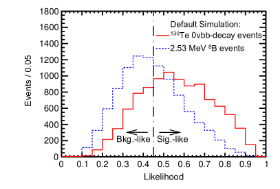
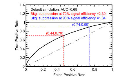
Figure 4: [Left]: The distribution of the likelihood values, $L$, calculated using Eq. 5 for 10,000 simulated 0$\nu\beta\beta$ signal (solid red line) and ⁸B background (dotted blue line) events. The vertical black dash-dotted line at 0.45 corresponds to a cut on the likelihood value that results in 70% signal efficiency. The default simulation settings are used. [Right]: The true positive rate $TPR(L_{cut})$ as a function of the false positive rate $FPR(L_{cut})$, or the ROC-curve. Using the ROC-curve we determine that the background suppression factor is 2.30 at 70% signal efficiency (dashed red lines) and 1.34 at 90% signal efficiency (dotted blue lines). The AUC for this ROC-curve is 0.69. The horizontal black thin solid line at $TPR=$1 corresponds to an ideal event classification algorithm with 100% separation between signal and background (AUC=1); the black dash-dotted diagonal line corresponds to a classification algorithm based on a random guess with no separation between signal and background (AUC=0.5).

4.3 Event Classification Results

Introducing a likelihood threshold, $L_{cut}$, in the likelihood distribution $p(2e|\vec{S}_{meas})$, we can classify an event with a likelihood $p(2e|\vec{S}_{meas})>L_{cut}$ to be a signal event. We scan over $L_{cut}$ values to determine the background suppression factors at a signal efficiencies of 70% and 90%. For example, for the likelihood distribution shown on the left-hand panel of Fig. 4, 70% signal efficiency corresponds to the $L_{cut}$ value of 0.45. Rejecting events with $p(2e|\vec{S}_{meas})<0.45$ results in rejecting 56.5% of the simulated ⁸B background events, i.e. a background suppression factor of 2.3.

For any given value of the likelihood threshold $L_{cut}$, we define the true positive rate (TPR) as a fraction of signal events that satisfy $p(2e|\vec{S}_{meas})>L_{cut}$. In other words, the TPR is a fraction of signal events that are correctly classified as signal. The TPR is the signal efficiency.

Similarly, we define the false positive rate (FPR) as a fraction of background events that satisfy $p(2e|\vec{S}_{meas})>L_{cut}$. In other words, the FPR is a fraction of background events that are falsely classified as signal. The inverse value of the FPR, $\frac{1}{FPR}$, is the background suppression factor.

The true positive rate (TPR) as a function of the false positive rate (FPR) is known as the receiver operating characteristic curve (ROC-curve). The ROC-curve is commonly used in computer science to characterize the performance of a classification algorithm.

The right-hand panel on Fig. 4 shows the ROC-curve, $TPR=f(FPR)$, corresponding to the topological reconstruction for the default simulation. For comparison, the ROC-curve of a perfect reconstruction is shown as a horizontal line at $TPR=1$. The ROC-curve of a classification algorithm based on a random guess is shown as a diagonal line, $TPR=FPR$.

We use the area under the ROC-curve (AUC) as a figure of merit to numerically characterize the performance of the topological reconstruction. The AUC of 0.5 corresponds to no separation between signal and background. The AUC of 1 corresponds to a perfect separation between signal and background. For the topological reconstruction shown in Fig. 4 (right) the AUC is 0.69. The background suppression factor is 2.30 and 1.34 at 70% and 90% signal efficiency respectively.

Figure 5 shows the dependence of the topological reconstruction on the photo-coverage. We vary the photo-coverage in the default simulation from 10% to 100%. For 100% coverage the AUC is 0.71 and the background suppression factors are 1.38 and 2.44 at 90% and 70% signal efficiency respectively. At 10% coverage the AUC and the background suppression factors drop to 0.59, 1.21, and 1.69, respectively.

We note that the default simulation with 100% photo-coverage matches the simulation settings used in the previously published spherical harmonics analysis [22]. Therefore, the background suppression factor of 2.44 can be directly compared with the factor of about 2.0 for the technique described in Ref. [22] . The topological reconstruction presented here leads to a more than 20% improvement in background suppression at 70% signal efficiency.

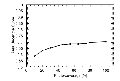
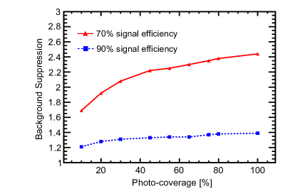
Figure 5: [Left]: The area under the curve (AUC) as a function of the photo-coverage. Each point is calculated based on the likelihood distributions of 10,000 0$\nu\beta\beta$ signal and ⁸B background events simulated with all the default simulation settings except for the photo-coverage, which is varied from 10% to 100%. [Right]: The background suppression factors at 70% signal efficiency (solid red line) and 90% signal efficiency (dotted blue line) as a function of the vertex smearing. Each point is calculated based on the ROC curve of 10,000 0$\nu\beta\beta$ signal and ⁸B background events simulated with all the default simulation settings except for the vertex smearing, which is varied from 10% to 100%.

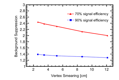
Figure 6: [Left]: The area under the curve (AUC) as a function of the vertex smearing, $\sigma_{r_{v}}$. Each point is calculated based on the likelihood distributions of 10,000 0$\nu\beta\beta$ signal and ⁸B background events simulated with all the default simulation settings except for the vertex smearing, which is varied from 2.6 cm to 12.1 cm (this corresponds to 1.5-7 cm range in $\sigma_{x,y,z}$). [Right]: The background suppression with 70% signal efficiency (solid red line) and 90% signal efficiency (dotted blue line) as a function of the vertex smearing, $\sigma_{r_{v}}$. Each point is calculated based on the ROC curve of 10,000 0$\nu\beta\beta$ signal and ⁸B background events simulated with all the default simulation settings except for the vertex smearing, which is varied from 2.6 cm to 12.1 cm (this corresponds to 1.5-7 cm range in $\sigma_{x,y,z}$).

We also considered a detector simulation with an ideal light collection: both photo-coverage and QE are 100%, while all other parameters are the same as in the default simulation. For this scenario, we find the background suppression factors of 1.56 and 3.57 at 90% and 70% signal efficiency respectively.

We find a similar performance of the topological reconstruction for a scenario where we change the photo-coverage back to the default 65%, remove all scintillation light, and filter Cherenkov PEs through a uniform QE of 30%. For this scenario we find the background suppression factors of 1.59 and 3.39 at 90% and 70% signal efficiency respectively. This emphasizes the importance of further developments in techniques to separate Cherenkov PEs from scintillation PEs.

We also study the dependence of the topological reconstruction on the vertex resolution. Using the default simulation with 65% photo-coverage we vary the vertex smearing from $\sigma_{r_{v}}$ = 2.6 cm ($\sigma_{x,y,z}$ = 1.5 cm) to $\sigma_{r_{v}}$ = 12.1 cm ($\sigma_{x,y,z}$ = 7 cm). Figure 6 shows the AUC and the background suppression factors as a function of vertex smearing. Improvements in the vertex resolution lead to a better performance of the topological reconstruction.

5 Directionality Reconstruction

The topological reconstruction discussed in Sec. 4 cannot distinguish signal and background events if in signal events the two electrons are emitted at a small angle or if one electron is emitted with kinetic energy below Cherenkov threshold. However, electron directionality provides an extra handle to separate ⁸B background from $0\nu\beta\beta$-decay signal events that are misidentified as one-track events. The direction of the electron in a ⁸B background event is correlated with the direction to the Sun, while the directions of the electrons in a 0$\nu\beta\beta$ signal event do not have such correlation. Therefore, ⁸B background can be further suppressed by reconstructing the directionality of one-track candidate events.

We reconstruct the direction of the electron $\hat{r}_{e}$ using the average of the weighted unit hit vector $\frac{\vec{r}_{i}-\vec{r}_{v}}{\absolutevalue{\vec{r}_{i}-\vec{r}_{v}}}$ of the PEs from the vertex $\vec{r}_{v}$:

$$\hat{r}_{e}=\frac{\sum_{i=1}^{N_{PE}}W(t_{i},\theta_{i})\frac{\vec{r}_{i}-\vec{r}_{v}}{\absolutevalue{\vec{r}_{i}-\vec{r}_{v}}}}{\absolutevalue{\sum_{i=1}^{N_{PE}}W(t_{i},\theta_{i})\frac{\vec{r}_{i}-\vec{r}_{v}}{\absolutevalue{\vec{r}_{i}-\vec{r}_{v}}}}}$$ (6)

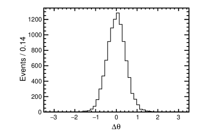
Figure 7: Comparison between reconstructed and true direction of the electron $\hat{r}_{e}$. Simulation of 10,000 one-track ⁸B background events with the default simulation settings. [Left]: Difference between reconstructed and true polar angle $\Delta\theta=\theta_{reco}-\theta_{true}$. The RMS value of the $\Delta\theta$ distribution is 0.46. [Right]: Difference between reconstructed and true azimuthal angle $\Delta\phi=\phi_{reco}-\phi_{true}$. The RMS value of the $\Delta\phi$ distribution is 0.84.

Figure 7 shows the comparison between the reconstructed and the true direction of the electron. The distribution of the difference between the reconstructed and the true polar angle, $\Delta\theta=\theta_{reco}-\theta_{true}$, has an RMS value of 0.46. The distribution of the difference between the reconstructed and the true azimuthal angle, $\Delta\phi=\phi_{reco}-\phi_{true}$, has an RMS value of 0.84.

As in Ref. [20] we also use the inner product between the reconstructed electron direction and the true electron direction as a figure of merit for directionality reconstruction. The left-hand panel in Fig. 8 shows the inner product between the reconstructed electron direction and the true electron direction. The mean value of the distribution shown in Fig. 8 (left) is 0.78, where the mean inner product of 1 would correspond to perfect directionality reconstruction.

The right-hand panel in Fig. 8 shows the mean value of the inner product distribution as a function of photo-coverage. As expected, the inner product increases with larger photo-coverage.

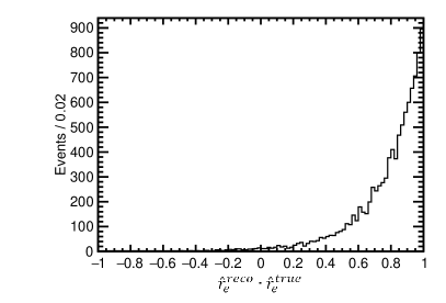
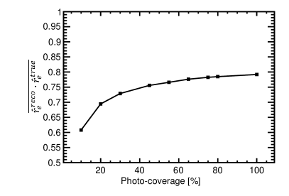
Figure 8: [Left]: The inner product between the reconstructed direction and the true electron direction for simulation of 10,000 one-track ⁸B background events with the default simulation settings. [Right]: The mean value of the inner product distribution as a function of photo-coverage. The default simulation settings are used except for the photo-coverage, which is varied from 10% to 100%.

To estimate the improvements in the directionality reconstruction in the absence of scintillation light we apply the technique to a sample of Cherenkov PEs filtered through a uniform QE of 30% independent of a wavelength and the default photo-coverage of 65%. We find that the directionality reconstruction resolution improves from 0.46 to 0.40 radians and from 0.84 to 0.74 radians for the polar angle and azimuthal angles respectively. The inner product improves from 0.78 to 0.83.

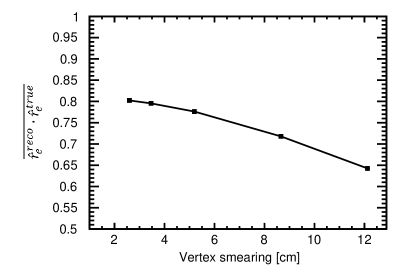
Figure 9: The mean value of the inner product distribution as a function of vertex smearing, $\sigma_{r_{v}}$. The default simulation settings are used except for the vertex smearing, which is varied from 2.6 cm to 12.1 cm. (this corresponds to 1.5-7 cm range in $\sigma_{x,y,z}$).

These improvements are very similar to the case of an ideal light collection. Assuming both photo-coverage and QE of 100% and keeping all other parameters are the same as in the default simulation, we find the inner product of 0.84. The RMS values of $\Delta\theta=\theta_{reco}-\theta_{true}$ and $\Delta\phi=\phi_{reco}-\phi_{true}$ are 0.39 and 0.72 respectively.

To study the dependence of the directionality reconstruction on the vertex resolution, we run the default simulation at different vertex smearing. Figure 9 shows the mean value of the inner product between the reconstructed electron direction and the true electron direction as a function of vertex smearing. The directionality reconstruction degrades as the vertex smearing increases.

Table 1 summarizes the performance of topological and directional reconstruction for different detector simulation settings.

Simulation scenario	Photo-coverage [%]	$QE_{che}$ [%]	$QE_{sci}$ [%]	AUC	$\frac{1}{FPR@90\%}$	$\frac{1}{FPR@70\%}$	$\overline{\hat{r}_{e}^{reco}\cdot\hat{r}_{e}^{true}}$	$RMS_{\theta}$	$RMS_{\phi}$
Default simulation	65	12	23	0.69	1.34	2.30	0.78	0.46	0.84
Ideal light collection	100	100	100	0.78	1.56	3.57	0.84	0.39	0.72
Cherenkov PEs only	65	30	0	0.77	1.59	3.39	0.83	0.40	0.74
Same as in Ref. [22]	100	12	23	0.71	1.38	2.44	0.79	0.45	0.81

Table 1: Results of topological and directional reconstruction for different simulation settings. Only photo-coverage and QE deviate from the default simulation; $QE_{che}$ and $QE_{sci}$ are averaged QE for Cherenkov and scintillation light respectively. For the topological reconstruction we list the area under the curve as well as background suppression factors, $\frac{1}{FPR}$, at 90% and 70% signal efficiency. For the directionality reconstruction we list the value of the inner product and the value of RMS of the distributions of the difference between the reconstructed and the true polar and azimuthal angles.

6 Conclusions

We have presented a technique to separate $0\nu\beta\beta$-decay events from ⁸B solar neutrino background in a large liquid scintillator detector. We introduce the Cherenkov-scintillation space-time boundary to increase the contribution from the Cherenkov PEs in the reconstruction of the kinematics of candidate events. The technique has two components. The first component of the technique is the reconstruction of the event topology that allows the separation of the two-track event topology of $0\nu\beta\beta$-decay signal events from one-track ⁸B background events. The second component is the reconstruction of the directionality of the one-electron candidate events that allows for the further suppression of ⁸B background due to the correlation between the direction of scattered electron in ⁸B events and the position of the sun. The directionality reconstruction should be applied after the event topology reconstruction which determines that the topology of a candidate event is consistent with the one-track event topology.

We evaluated the performance of the topological and directionality reconstruction separately. For the default detector model with 65% photo-coverage and assuming vertex resolution of $\sigma_{r_{v}}=$ 5.2 cm, the method of reconstructing the event topology predicts factors of 1.3 and 2.3 in background suppression at 90% and 70% signal efficiency respectively based solely on the reconstruction of the event topology. For the reconstruction of electron directionality we estimate the polar angular resolution to be 0.49 radians and the azimuthal angular resolution to be 0.84 radians. The determination of a combined effect on the sensitivity to the $0\nu\beta\beta$-decay half-time is a subject of further studies using a detailed detector-specific background model.

For a photo-cathode spectral response modeled after KamLAND PMTs, an increase in photo-coverage beyond 65% does not lead to significant improvements in the performance of the topological and directionality reconstruction. At the same time an increase in the collection efficiency of Cherenkov PEs relative to scintillation PEs leads to about 50% higher background suppression factor at 70% signal efficiency for the topological reconstruction.

Separation of Cherenkov PEs from scintillation PEs is essential for topological and directionality reconstruction in a liquid scintillator detector. The introduced Cherenkov-scintillation space-time boundary provides a mechanism for selecting a sample of the early emitted PEs containing a high fraction of the Cherenkov PEs. The effectiveness of the Cherenkov-scintillation space-time boundary in selecting a PE sample with high fraction of Cherenkov PEs depends on properties of liquid scintillator and performance of light collection system.

Performance of the technique presented in this paper can be improved by developing new liquid scintillators and new light collection systems. Liquid scintillators need to have a narrower emission spectrum shifted to shorter wavelengths and a longer rise time. Light collection systems should include large-area photo-detectors with mm space and 100-psec time resolutions, and red-sensitive photo-cathode. Spectral sorting of photons can minimize the effect of chromatic dispersion and further improve the performance of the technique.

7 Acknowledgements

We acknowledge contribution by Lindley Winslow to the earlier version of the algorithm separating $0\nu\beta\beta$-decay and ⁸B events, and AE thanks her for many productive discussions on the event topology reconstruction. We thank Roy Garcia for performing independent cross-checks of calculations related to the spherical harmonics analysis. We thank Henry Frisch for reading this manuscript and providing comments. We thank Evan Angelico, Eric Spieglan, and Chuck Whitmer for feedback and comments. We thank Alexander Bogatskii for discussions on rotation invariants of the SO(3) group. We thank Jo$\tilde{a}$o Shida for proof reading. AE thanks Ed Blucher, Andy Mastbaum, and Tony LaTorre for discussions on properties of liquid scintillators. This work is supported by U. S. Department of Energy, Office of Science, Offices of High Energy Physics and Nuclear Physics under contracts DE-SC0008172 and DE-SC0015367; the National Science Foundation under grant PHY-1066014; and the Physical Sciences Division of the University of Chicago. This research was done using resources provided by the Open Science Grid [57, 58], which is supported by the National Science Foundation award 1148698, and the U.S. Department of Energy’s Office of Science.

Appendix A Detector Coverage Scheme

To uniformly distribute photo-detectors over a sphere, we assign a photo-detector at each vertex of a platonic solid (i.e., tetrahedron, cube, octahedron, dodecahedron and icosahedron). The assigned photo-detectors will be uniformly distributed over the circumscribed sphere of the platonic solid. However, there is no exact solution for distributing more than 20 points over a sphere.

To approximate a uniform distribution of more than 20 photo-detectors over the sphere, we assign additional photo-detectors to the edges and the faces of the platonic solids and project the photo-detectors onto the circumscribed sphere.

We start with a icosahedron for its largest number of faces among the platonic solids. We equally divide each edge by $N$ times and consequently divide each triangular face by $N^{2}$ times.

We introduce the following coordinate system. Starting from one vertex of a face, we define the directions along the two edges to be unit vectors $\vec{e}_{1}$ and $\vec{e}_{2}$. We also define the length of each division to be 1. Consequently, all the intersecting points in the Figure 10 have unique integer coordinates $(x,y)$ under the basis of $\vec{e}_{1}$ and $\vec{e}_{2}$. We select all the points that satisfy $x\equiv y\pmod{3}$.

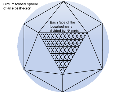
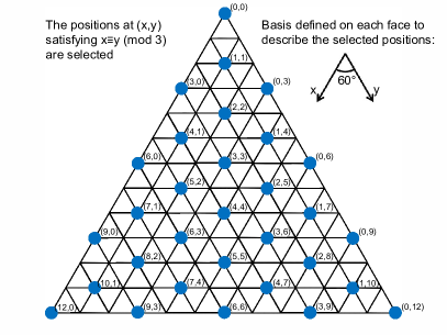
Figure 10: [Top left]: An icosahedron circumscribed by a sphere. We subdivide each face by $N^{2}$ times (where $N\equiv 0(mod3)$) and select some particular positions on each face and project the positions onto the circumscribed sphere to enable the assignment of more detectors. [Top Right]: The selection of the detectors on each face on the icosahedron before the projection. We assign detectors to all the positions with coordinates $(x,y)$ satisfying $x\equiv y(mod3)$. [Bottom Left]: An illusration of tuning the positions of the detectors. The triangles are rescaled such that the vertices of the triangles are equally spaced over the sphere. Furthermore, the geodesic projected from $A_{n}B_{n}$ $B_{n}C_{n}$ $C_{n}A_{n}$ are respectively equally partitioned by $n$ times. [Bottom Right]: The positions of the detectors over the sphere projected from one face of the icosahedron, given the subdivision number $N=48$.

However, for such selection, the distance between two closest projected points near the vertex is smaller than the distance between two closest projected points near the center of the face (see Figure 10).

Therefore, in order to space the points more uniformly, we first partition all the points by classes of triangles (see Figure 10, the triangles with the thickened line width are the subdivided triangle classes). Notice that any straight lines in $\mathbb{R}^{3}$ projected onto a sphere $S^{2}$ are geodesics; therefore, the projected triangle classes onto the sphere are geodesic triangles, regardless of the size of the triangle.

While fixing the common centroid of these triangle classes unchanged, we scale all the triangle classes such that the vertices of these triangle classes are equally spaced along the geodesics that connect the icosahedron vertex and the common centroid. Meanwhile, given the total number of points along each edge of the subdivided triangle class remains unchanged, we reassign the location of the points along each edge of each subdivided triangle, such that the points are equally spaced along the edge of each triangle class after being projected onto the circumscribed sphere (see Figure 10).

Appendix B Spherical Harmonics Analysis

B.1 S-spectrum $S_{\ell}$

Suppose an angular function $f(\theta,\phi)$ on a unit sphere $\mathbb{S}^{2}$ represents the angular distribution of photo-electrons (PE) over the detector surface. Such angular function $f(\theta,\phi)$ has a corresponding spherical harmonics expansion:

$$f(\theta,\phi)=\sum_{\ell=0}^{+\infty}\sum_{m=-\ell}^{\ell}f_{\ell m}Y_{\ell m}(\theta,\phi)$$ (7)

where $Y_{\ell m}(\theta,\phi)$ are tesseral harmonics (real-valued spherical harmonics), which form a complete orthonormal basis of the rigged Hilbert space (all real square integrable functions and Dirac delta functions defined over $S^{2}$):

$$Y_{\ell m}(\theta,\phi)=\left\{\begin{array}[]{@{}ll@{}}\sqrt{2}\sqrt{\frac{(2\ell+1)}{4\pi}\frac{(\ell-m)!}{(\ell+m)!}}P_{\ell}^{m}(\cos\theta)\cos~{}m\phi&,\text{if}\ m>0\\ \sqrt{\frac{(2\ell+1)}{4\pi}\frac{(\ell-m)!}{(\ell+m)!}}P_{\ell}^{m}(\cos\theta)&,\text{if}\ m=0\\ \sqrt{2}\sqrt{\frac{(2\ell+1)}{4\pi}\frac{(\ell-m)!}{(\ell+m)!}}P_{\ell}^{|m|}(\cos\theta)\sin~{}|m|\phi&,\text{if}\ m<0\end{array}\right.$$ (11)

and the projection coefficients $f_{\ell m}$ are given by the projection of $f(\theta,\phi)$ onto the basis $Y_{\ell m}(\theta,\phi)$:

$$f_{\ell m}=\int_{0}^{\pi}\sin\theta d\theta\int_{0}^{2\pi}d\phi f(\theta,\phi)Y_{\ell m}(\theta,\phi)$$ (12)

For a given angular functuion $f(\theta,\phi)$, its rotationally invariant S-spectrum $S_{\ell}$ is defined as:

$$S_{\ell}=\sum_{m=-\ell}^{\ell}|f_{\ell m}|^{2}$$ (13)

B.2 Weighted Angular Distribution $f(\theta,\phi)$ of Photo-electrons

Suppose the Dirac delta function $\delta(\cos\theta-\cos\theta_{i})\delta(\phi-\phi_{i})$ represents the angular distribution of an individual PE at a location with coordinates $(\theta_{i},\phi_{i})$ on the detector surface. The $L^{1}$-normalized (see Equation 17) weighted angular distribution $f(\theta,\phi)$ of all $N_{PE}$ photo-electrons (PEs) is

$$f(\theta,\phi)=\frac{\sum_{i=1}^{N_{PE}}W(t_{i},\theta_{i})\delta(\cos\theta-\cos\theta_{i})\delta(\phi-\phi_{i})}{\sum_{i=1}^{N_{PE}}W(t_{i},\theta_{i})}$$ (14)

Substituting the distribution $f(\theta,\phi)$ into the Equation 12 yields the corresponding projection coefficients $f_{\ell m}$:

$$f_{\ell m}=\int_{0}^{\pi}\sin\theta d\theta\int_{0}^{2\pi}d\phi\frac{\sum_{i=1}^{N_{PE}}W(t_{i},\theta_{i})\delta(\cos\theta-\cos\theta_{i})\delta(\phi-\phi_{i})}{\sum_{i=1}^{N_{PE}}W(t_{i},\theta_{i})}Y_{\ell m}(\theta,\phi)=\frac{\sum_{i=1}^{N_{PE}}W(t_{i},\theta_{i})Y_{\ell m}(\theta_{i},\phi_{i})}{\sum_{i=1}^{N_{PE}}W(t_{i},\theta_{i})}$$ (15)

and also its S-spectrum $S_{\ell}$:

$$S_{\ell}=\sum_{m=-\ell}^{\ell}\absolutevalue{f_{\ell m}}^{2}=\sum_{m=-\ell}^{\ell}\absolutevalue{\frac{\sum_{i=1}^{N_{PE}}W(t_{i},\theta_{i})Y_{\ell m}(\theta_{i},\phi_{i})}{\sum_{i=1}^{N_{PE}}W(t_{i},\theta_{i})}}^{2}=\frac{\sum_{m=-\ell}^{\ell}\absolutevalue{\sum_{i=1}^{N_{PE}}W(t_{i},\theta_{i})Y_{\ell m}(\theta_{i},\phi_{i})}^{2}}{\absolutevalue{\sum_{i=1}^{N_{PE}}W(t_{i},\theta_{i})}^{2}}$$ (16)

B.3 Normalization of the Angular Distribution $f(\theta,\phi)$

In this paper, the angular distribution of PEs, $f(\theta,\phi)$, is normalized by the $L^{1}$ norm:

$$||f(\theta,\phi||_{1}=\int_{S^{2}}d\Omega\absolutevalue{f(\theta,\phi)}$$ (17)

For example, the $L^{1}$ norm of the weighted angular distribution $f(\theta,\phi)=\sum_{i=1}^{N_{PE}}W(t_{i},\theta_{i})\delta(\cos\theta-\cos\theta_{i})\delta(\phi-\phi_{i})$, which is not yet normalized, is $\sum_{i=1}^{N_{PE}}W(t_{i},\theta_{i})$. As a consequence, in this paper, all the S-spectra has the normalization factor $\absolutevalue{\sum_{i=1}^{N_{PE}}W(t_{i},\theta_{i})}^{2}$ in the denominator.

Note, the sum of $S_{\ell}$’s over all multiple moments $\ell$ equals to the $L^{2}$ norm of the function $f(\theta,\phi)$:

$$||f(\theta,\phi||_{2}=\int_{S^{2}}d\Omega|f(\theta,\phi)|^{2}=\sum_{\ell=0}^{+\infty}S_{\ell}$$ (18)

However, the detection signal $f(\theta,\phi)$ in this paper, which is a weighted sum of the Dirac delta functions, is not square integrable; as a consequence, the sum of $S_{\ell}$’s diverges.

B.4 Rotation Invariance of the S-spectrum

To simplify the notation in the following proof, we adopt the Dirac bracket notation: $\ket{f}=f(\theta,\phi)$ and $\ket{Y_{\ell m}}=Y_{\ell m}(\theta,\phi)$.

We define operators $\hat{L}_{x}$, $\hat{L}_{y}$, $\hat{L}_{z}$, $\hat{L}^{2}$, $\hat{R}$ to be:

$$\left\{\begin{array}[]{@{}ll@{}}\hat{L}_{x}=y\partial_{z}-z\partial_{y}=-\sin\phi\partial_{\theta}-\cot\theta\cos\phi\partial_{\phi}\\ \hat{L}_{y}=z\partial_{x}-x\partial_{z}=\cos\phi\partial_{\theta}-\cot\theta\sin\phi\partial_{\phi}\\ \hat{L}_{z}=x\partial_{y}-y\partial_{x}=\partial_{\phi}\\ \hat{L}^{2}=\frac{\partial_{\theta}(\sin\theta\partial_{\theta})}{\sin\theta}+\frac{\partial^{2}_{\phi}}{\sin^{2}\theta}\\ \hat{R}=\hat{R}^{\prime}_{z}\hat{R}_{x}\hat{R}_{z}=e^{L_{z}\Delta\phi_{z}^{\prime}}e^{L_{x}\Delta\phi_{x}}e^{L_{z}\Delta\phi_{z}}\end{array}\right.$$ (24)

The tesseral harmonics $\ket{Y_{\ell m}}$ (real-valued spherical harmonics) are the eigenvectors of $\hat{L}^{2}$: $\hat{L}^{2}\ket{Y_{\ell m}}=\ell(\ell+1)\ket{Y_{\ell m}}$. The collection of the tesseral harmonics forms a complete orthonormal basis of the rigged Hilbert space $\mathscr{H}$ over $\mathbb{S}^{2}$. We define $\mathscr{H}_{\ell}$ to be a subspace of the space $\mathscr{H}$, which is spanned by the eigenvectors $\ket{Y_{\ell m}}$ with a given fixed $\ell$. The collection of $\ket{Y_{\ell m}}$ with a given fixed $\ell$ forms a complete orthonormal basis of $\mathscr{H}_{\ell}$. Therefore, the operator $\sum_{m=-\ell}^{+\ell}\ket{Y_{\ell m}}\bra{Y_{\ell m}}$ is equivalent to the identity operator $\hat{I}_{\ell}$ in $\mathscr{H}_{\ell}$ (and equivalent to 0 in the other subspaces $\mathscr{H}_{\ell^{\prime}}$ with $\ell^{\prime}\neq\ell$).

$[\hat{L}_{i},\hat{L}^{2}]=0$ leads to $[\hat{R}_{i},\hat{L}^{2}]=0$ and $[\hat{R},\hat{L}^{2}]=0$. Therefore, $\hat{R}\ket{Y_{\ell m}}$ is an eigenstate of $\hat{L}^{2}$ in $\mathscr{H}_{\ell}$.

Using the Dirac bracket notation, we rewrite the definition of the S-spectrum $S_{\ell}$:

$$S_{\ell}=\sum_{m=-\ell}^{+\ell}\absolutevalue{f_{\ell m}}^{2}=\sum_{m=-\ell}^{+\ell}\bra{f}\ket{Y_{\ell m}}\bra{Y_{\ell m}}\ket{f}$$ (25)

Applying an arbitrary rotation $\hat{R}$ to the detection signal $\ket{f^{\prime}}=\hat{R}\ket{f}$, the S-spectrum $S_{\ell}$ is transformed to be $S_{\ell}^{\prime}$:

$$S_{\ell}^{\prime}=\sum_{m=-\ell}^{+\ell}\absolutevalue{f^{\prime}_{\ell m}}^{2}=\sum_{m=-\ell}^{+\ell}\bra{f^{\prime}}\ket{Y_{\ell m}}\bra{Y_{\ell m}}\ket{f^{\prime}}=\sum_{m=-\ell}^{+\ell}\bra{f}\hat{R}^{\dagger}\ket{Y_{\ell m}}\bra{Y_{\ell m}}\hat{R}\ket{f}$$ (26)

Applying spectral decomposition to $\ket{f}$ and organizing:

$$S_{\ell}^{\prime}=\sum_{m=-\ell}^{+\ell}\sum_{\ell^{\prime}m^{\prime}}\sum_{\ell^{\prime\prime}m^{\prime\prime}}f_{\ell^{\prime}m^{\prime}}f_{\ell^{\prime\prime}m^{\prime\prime}}\bra{Y_{\ell^{\prime}m^{\prime}}}\hat{R}^{\dagger}\ket{Y_{\ell m}}\bra{Y_{\ell m}}\hat{R}\ket{Y_{\ell^{\prime\prime}m^{\prime\prime}}}$$ (27)

Recall $\hat{R}\ket{Y_{\ell m}}$ is an eigenstate of $\hat{L}^{2}$ in $\mathscr{H}_{\ell}$. Therefore, $\bra{Y_{\ell m}}\hat{R}\ket{Y_{\ell^{\prime\prime}m^{\prime\prime}}}$ is non-zero, if $\ell^{\prime\prime}=\ell$. Similarly, $\bra{Y_{\ell m}}\hat{R}\ket{Y_{\ell^{\prime}m^{\prime}}}$ is non-zero, if $\ell^{\prime}=\ell$. Consequently, the only non-zero term in the sum above is

$$S_{\ell}^{\prime}=\sum_{m^{\prime},m^{\prime\prime}}f_{\ell m^{\prime}}f_{\ell m^{\prime\prime}}\bra{Y_{\ell m^{\prime}}}\hat{R}^{\dagger}\sum_{m=-\ell}^{+\ell}\ket{Y_{\ell m}}\bra{Y_{\ell m}}\hat{R}\ket{Y_{\ell m^{\prime\prime}}}$$ (28)

Recall $\sum_{m=-\ell}^{+\ell}\ket{Y_{\ell m}}\bra{Y_{\ell m}}$ is equivalent to the identity operator, when applying to any vectors in $\mathscr{H}_{\ell}$. Therefore, the equation above can be simplified:

$$S_{\ell}^{\prime}=\sum_{m^{\prime},m^{\prime\prime}}f_{\ell m^{\prime}}f_{\ell m^{\prime\prime}}\bra{Y_{\ell m^{\prime}}}\hat{R}^{\dagger}\hat{I}_{\ell}\hat{R}\ket{Y_{\ell m^{\prime\prime}}}=\sum_{m^{\prime},m^{\prime\prime}}f_{\ell m^{\prime}}f_{\ell m^{\prime\prime}}\bra{Y_{\ell m^{\prime}}}\ket{Y_{\ell m^{\prime\prime}}}=\sum_{m^{\prime},m^{\prime\prime}}f_{\ell m^{\prime}}f_{\ell m^{\prime\prime}}\delta_{m^{\prime}m^{\prime\prime}}=\sum_{m^{\prime}}f_{\ell m^{\prime}}f_{\ell m^{\prime}}$$ (29)

Changing the label $m^{\prime}$ to $m$, we prove the rotation invariance of the S-spectrum $S_{\ell}$:

$$S_{\ell}^{\prime}=\sum_{m}f_{\ell m}f_{\ell m}=\sum_{m}\absolutevalue{f_{\ell m}}^{2}=S_{\ell}$$ (30)

Appendix C Maximum Likelihood Estimation

C.1 Conditional Probability Distribution

For an arbitrary event, given its measurement $\vec{S}_{meas}=(S_{1},\alpha)$ in the parameter space of $(S_{1},\alpha)$, the likelihood for the event to be a signal (0$\nu\beta\beta$, $2e$) is the conditional probability $p(1e|\vec{S}_{meas})$. Similarly, the likelihood for the event to be a background (solar neutrino interaction, $1e$) is the conditional probability $p(2e|\vec{S}_{meas})$. Based on Baysian theorem, these posterior probabilities are given by:

$$\left\{\begin{array}[]{@{}ll@{}}p(1e|\vec{S}_{meas})&=\frac{p(1e)}{p(\vec{S}_{meas})}p(\vec{S}_{meas}|1e)=k_{1}p(\vec{S}_{meas}|1e)\\ p(2e|\vec{S}_{meas})&=\frac{p(2e)}{p(\vec{S}_{meas})}p(\vec{S}_{meas}|2e)=k_{2}p(\vec{S}_{meas}|2e)\end{array}\right.$$ (33)

where the response function $p(\vec{S}_{meas}|1e)$ ($p(\vec{S}_{meas}|2e)$) is the conditional probability of getting measurement $\vec{S}_{meas}$ given the event is a 0$\nu\beta\beta$ signal (⁸B background), which can be read from the histograms in the Figure 3. The coefficients $k_{1}$ and $k_{2}$ are determined by the ratio of the prior probabilities $p(1e):p(2e)$ and the normalization. In this paper, the ratio of the prior probabilities ${k_{1}}:{k_{2}}={p(1e)}:{p(2e)}$ is set to be 1.

$$\left\{\begin{array}[]{@{}ll@{}}{k_{1}}:{k_{2}}={p(1e)}:{p(2e)}=1\\ k_{1}p(\vec{S}_{meas}|1e)+k_{2}p(\vec{S}_{meas}|2e)=1\end{array}\right.$$ (36)

Therefore, through solving the four equations in the Equation 33 and 36, the posterior probabilities $p(1e|\vec{S}_{meas})$ and $p(2e|\vec{S}_{meas})$ are given by

$$\left\{\begin{array}[]{@{}ll@{}}p(1e|\vec{S}_{meas})&=\frac{p(\vec{S}_{meas}|1e)}{p(\vec{S}_{meas}|1e)+p(\vec{S}_{meas}|2e)}\\ p(2e|\vec{S}_{meas})&=\frac{p(\vec{S}_{meas}|2e)}{p(\vec{S}_{meas}|1e)+p(\vec{S}_{meas}|2e)}\end{array}\right.$$ (39)

C.2 Multi-dimensional Probability Distribution

In practice, filling the histograms of $p(s_{1},\alpha|1e)$ and $p(s_{1},\alpha|2e)$ requires more data than filling the histograms of $p(s_{1}|1e)$, $p(\alpha|1e)$, $p(s_{1}|2e)$ and $p(\alpha|2e)$. Given limited data, we replace these multi-dimensional histograms by the product of multiple 1-dimensional histograms:

$$\left\{\begin{array}[]{@{}ll@{}}p(S_{1},\alpha|1e)\approx p(S_{1}|1e)p(\alpha|1e)\\ p(S_{1},\alpha|2e)\approx p(S_{1}|2e)p(\alpha|2e)\end{array}\right.$$ (42)

Based on the approximation above, the probabilities in the Equation 39 become:

$$p(2e|\vec{S}_{meas})=\frac{p(\vec{S}_{meas}|2e)}{p(\vec{S}_{meas}|1e)+p(\vec{S}_{meas}|2e)}=\frac{p(S_{1}|2e)p(\alpha|2e)}{\sum_{j=1}^{2}p(S_{1}|je)p(\alpha|je)}$$ (43)

References

- Majorana [1937] Ettore Majorana. Theory of the Symmetry of Electrons and Positrons. Nuovo Cim., 14:171–184, 1937. doi: 10.1007/BF02961314.
- Furry [1939] W. H. Furry. On transition probabilities in double beta-disintegration. Phys. Rev., 56:1184–1193, Dec 1939.
- Goeppert-Mayer [1935] M. Goeppert-Mayer. Double beta-disintegration. Phys. Rev., 48:512–516, 1935. doi: 10.1103/PhysRev.48.512.
- Duerr [2013] Michael Duerr. Lepton number violating new physics and neutrinoless double beta decay. Nucl. Phys. Proc. Suppl., 237-238:24–27, 2013. doi: 10.1016/j.nuclphysbps.2013.04.048.
- Schechter and Valle [1982] J. Schechter and J. W. F. Valle. Neutrinoless Double beta Decay in SU(2) x U(1) Theories. Phys. Rev., D25:2951, 1982. doi: 10.1103/PhysRevD.25.2951. [,289(1981)].
- Duerr et al. [2011] Michael Duerr, Manfred Lindner, and Alexander Merle. On the Quantitative Impact of the Schechter-Valle Theorem. JHEP, 06:091, 2011. doi: 10.1007/JHEP06(2011)091.
- Albert et al. [2014] J. B. Albert et al. Search for Majorana neutrinos with the first two years of EXO-200 data. Nature, 510:229–234, 2014. doi: 10.1038/nature13432.
- Gando et al. [2016] A. Gando et al. Search for Majorana Neutrinos near the Inverted Mass Hierarchy Region with KamLAND-Zen. Phys. Rev. Lett., 117(8):082503, 2016. doi: 10.1103/PhysRevLett.117.109903,10.1103/PhysRevLett.117.082503. [Addendum: Phys. Rev. Lett.117,no.10,109903(2016)].
- Agostini et al. [2018] M. Agostini et al. Improved limit on neutrinoless double- decay of from gerda phase ii. Phys. Rev. Lett., 120:132503, Mar 2018. doi: 10.1103/PhysRevLett.120.132503. URL https://link.aps.org/doi/10.1103/PhysRevLett.120.132503.
- Alvis et al. [2019] S. I. Alvis et al. A Search for Neutrinoless Double-Beta Decay in 76Ge with 26 kg-yr of Exposure from the MAJORANA DEMONSTRATOR. arXiv, 1902.02299, 2019.
- NSA [2015] 2015 NSAC Long Range Plan, 2015. URL http://science.energy.gov/~/media/np/nsac/pdf/2015LRP/2015_LRPNS_091815.pdf.
- Albert et al. [2018] J. B. Albert et al. Sensitivity and Discovery Potential of nEXO to Neutrinoless Double Beta Decay. Phys. Rev., C97(6):065503, 2018. doi: 10.1103/PhysRevC.97.065503.
- Abgrall et al. [2017] N. Abgrall et al. The Large Enriched Germanium Experiment for Neutrinoless Double Beta Decay (LEGEND). AIP Conf. Proc., 1894(1):020027, 2017. doi: 10.1063/1.5007652.
- Giuliani [2018] Andrea Giuliani. The Mid and Long Term Future of Neutrinoless Double Beta Decay, jun 2018. URL https://doi.org/10.5281/zenodo.1286915.
- Biller [2013] S. D. Biller. Probing Majorana neutrinos in the regime of the normal mass hierarchy. Phys. Rev. D, 87(7):071301, April 2013. doi: 10.1103/PhysRevD.87.071301.
- Reeder et al. [1993] R. A. Reeder et al. Dilute scintillators for large volume tracking detectors. Nucl. Instrum. Meth., A334:353–366, 1993. doi: 10.1016/0168-9002(93)90796-K.
- Smy [2007] Michael Smy. Low Energy Event Reconstruction and Selection in Super-Kamiokande-III. In Proceedings, 30th International Cosmic Ray Conference (ICRC 2007): Merida, Yucatan, Mexico, July 3-11, 2007, volume 5, pages 1279–1282, 2007. URL http://indico.nucleares.unam.mx/contributionDisplay.py?contribId=213&confId=4.
- Cravens et al. [2008] J. P. Cravens et al. Solar neutrino measurements in super-kamiokande-ii. Phys. Rev. D, 78:032002, Aug 2008. doi: 10.1103/PhysRevD.78.032002. URL https://link.aps.org/doi/10.1103/PhysRevD.78.032002.
- Winslow and Simpson [2012] L Winslow and R Simpson. Characterizing quantum-dot-doped liquid scintillator for applications to neutrino detectors. Journal of Instrumentation, 7:P07010, 2012. URL http://stacks.iop.org/1748-0221/7/i=07/a=P07010.
- Aberle et al. [2014] C. Aberle, A. Elagin, H. J. Frisch, M. Wetstein, and L. Winslow. Measuring directionality in double-beta decay and neutrino interactions with kiloton-scale scintillation detectors. J. Instrum., 9(06):P06012, 2014. URL http://stacks.iop.org/1748-0221/9/i=06/a=P06012.
- Andringa et al. [2016] S. Andringa et al. Current Status and Future Prospects of the SNO+ Experiment. Adv. High Energy Phys., 2016:6194250, 2016. doi: 10.1155/2016/6194250.
- Elagin et al. [2017] Andrey Elagin, Henry Frisch, Brian Naranjo, Jonathan Ouellet, Lindley Winslow, and Taritree Wongjirad. Separating Double-Beta Decay Events from Solar Neutrino Interactions in a Kiloton-Scale Liquid Scintillator Detector By Fast Timing. Nucl. Instrum. Meth., A849:102–111, 2017. doi: 10.1016/j.nima.2016.12.033.
- Alonso et al. [2014] J. R. Alonso et al. Advanced Scintillator Detector Concept (ASDC): A Concept Paper on the Physics Potential of Water-Based Liquid Scintillator. arXiv, 1409.5864, 2014.
- Caravaca et al. [2017a] J. Caravaca, F. B. Descamps, B. J. Land, J. Wallig, M. Yeh, and G. D. Orebi Gann. Experiment to demonstrate separation of Cherenkov and scintillation signals. Phys. Rev., C95(5):055801, 2017a. doi: 10.1103/PhysRevC.95.055801.
- Caravaca et al. [2017b] J. Caravaca, F. B. Descamps, B. J. Land, M. Yeh, and G. D. Orebi Gann. Cherenkov and Scintillation Light Separation in Organic Liquid Scintillators. Eur. Phys. J., C77(12):811, 2017b. doi: 10.1140/epjc/s10052-017-5380-x.
- Li et al. [2016] Mohan Li, Ziyi Guo, Minfang Yeh, Zhe Wang, and Shaomin Chen. Separation of scintillation and cherenkov lights in linear alkyl benzene. Nucl. Instrum. Meth., A830:303–308, 2016. doi: 10.1016/j.nima.2016.05.132.
- Gruszko et al. [2018] Julieta Gruszko, Brian Naranjo, Byron Daniel, Andrey Elagin, Diana Gooding, Chris Grant, Jonathan Ouellet, and Lindley Winslow. Detecting cherenkov light from 1-2 mev electrons in linear alkylbenzene. arXiv, 1811.11144, 2018.
- Guo et al. [2017] Ziyi Guo, Minfang Yeh, Rui Zhang, De-Wen Cao, Ming Qi, Zhe Wang, and Shaomin Chen. Slow Liquid Scintillator Candidates for MeV-scale Neutrino Experiments. arXiv, 1708.07781, 2017.
- Wang and Chen [2017] Zhe Wang and Shaomin Chen. Reveal the Mantle and K-40 Components of Geoneutrinos with Liquid Scintillator Cherenkov Neutrino Detectors. arXiv, 1709.03743, 2017.
- Zhi et al. [2018] Yu Zhi, Ye Liang, Zhe Wang, and Shaomin Chen. Wide field-of-view and high-efficiency light concentrator. Nucl. Instrum. Meth., A885:114–118, 2018. doi: 10.1016/j.nima.2017.12.003.
- Gooding et al. [2018] D. Gooding, J. Gruszko, C. Grant, B. Naranjo, and L. Winslow. Light Yield of Perovskite Nanocrystal-Doped Liquid Scintillator. arXiv, 1807.06634, 2018.
- Cumming et al. [2018] J. B. Cumming, S. Hans, and M. Yeh. Improving Light Yield Measurements for Low-Yield Scintillators. arXiv, 1810.02885, 2018.
- Kaptanoglu et al. [2018] Tanner Kaptanoglu, Josh Klein, and Meng Luo. Wavelength Dependence of LAB+PPO Emission Time. arXiv, 1811.11587, 2018.
- Fukuda [2016] Yoshiyuki Fukuda. ZICOS - New project for neutrinoless double beta decay experiment using zirconium complex in liquid scintillator. J. Phys. Conf. Ser., 718(6):062019, 2016. doi: 10.1088/1742-6596/718/6/062019.
- FUKUDA et al. [2018] Yoshiyuki FUKUDA, Yuto KAMEI, Narengerile, Akira OBATA, Shigetaka MORIYAMA, Izumi OGAWA, Takahiro GUNJI, Ryohei HAMAYA, and Satoru TSUKADA. Discrimination of cherenkov light in liquid scintillator for neutrinoless double beta decay experiment. Bulletin of Miyagi University of Education, 52:139–147, jan 2018. URL http://id.nii.ac.jp/1138/00000651/.
- Back et al. [2017] A. R. Back et al. Accelerator Neutrino Neutron Interaction Experiment (ANNIE): Preliminary Results and Physics Phase Proposal. arXiv, 1707.08222, 2017.
- Yeh et al. [2008] Minfang Yeh, Yuping Williamson, and Richard L. Hahn. Metal-loaded liquid scintillators for neutrino experiments. J. Phys. Conf. Ser., 136:042054, 2008. doi: 10.1088/1742-6596/136/4/042054.
- Yeh et al. [2011] M. Yeh, S. Hans, W. Beriguete, R. Rosero, L. Hu, R. L. Hahn, M. V. Diwan, D. E. Jaffe, S. H. Kettell, and L. Littenberg. A new water-based liquid scintillator and potential applications. Nucl. Instrum. Meth., A660:51–56, 2011. doi: 10.1016/j.nima.2011.08.040.
- Collaboration [2019] The ANNIE Collaboration. Private communication, 2019.
- Sakai [2016] Michinari Sakai. High Energy Neutrino Analysis at KamLAND and Application to Dark Matter Search. PhD thesis, Hawaii U., 2016. URL http://www.phys.hawaii.edu/~kamland/theses_and_dissertations/high_energy_neutrino_analysis_at_kamland_and_application_to_dark_matter_search.pdf.
- Dalmasson et al. [2018] Jacopo Dalmasson, Giorgio Gratta, Ako Jamil, Scott Kravitz, Milad Malek, Kevin Wells, Julie Bentley, Samuel Steven, and Jiani Su. Distributed Imaging for Liquid Scintillation Detectors. Phys. Rev., D97(5):052006, 2018. doi: 10.1103/PhysRevD.97.052006.
- Wonsak et al. [2018] Bjorn S. Wonsak, Caren I. Hagner, Dominikus A. Hellgartner, Kai Loo, Sebastian Lorenz, David J. Meyhöfer, Lothar Oberauer, Henning Rebber, Wladyslaw H. Trzaska, and Michael Wurm. Topological track reconstruction in unsegmented, large-volume liquid scintillator detectors. JINST, 13(07):P07005, 2018. doi: 10.1088/1748-0221/13/07/P07005.
- Li et al. [2018] Aobo Li, Andrey Elagin, Suzannah Fraker, Chris Grant, and Lindley Winslow. Suppression of Cosmic Muon Spallation Backgrounds in Liquid Scintillator Detectors Using Convolutional Neural Networks. arXiv, 1812.02906, 2018.
- Bonventre and Orebi Gann [2018] R. Bonventre and G. D. Orebi Gann. Sensitivity of a low threshold directional detector to CNO-cycle solar neutrinos. Eur. Phys. J., C78(6):435, 2018. doi: 10.1140/epjc/s10052-018-5925-7.
- Leyton et al. [2017] Michael Leyton, Stephen Dye, and Jocelyn Monroe. Exploring the hidden interior of the Earth with directional neutrino measurements. Nature Commun., 8:15989, 2017. doi: 10.1038/ncomms15989.
- Eguchi et al. [2003] K. Eguchi et al. Phys. Rev. Lett., 90:021802, Jan 2003.
- Ham [2013] Hamamatsu Photonics K.K., Large Photocathode Area Photomultiplier Tubes (data sheet, including R7081), accessed July 2013. http://www.hamamatsu.com/resources/pdf/etd/LARGE_ AREA_PMT_TPMH1286E05.pdf.
- Abe et al. [2012] Y. Abe et al. Phys. Rev., D86:052008, 2012. doi: 10.1103/PhysRevD.86.052008.
- Adams et al. [2015] Bernhard Adams et al. Timing characteristics of Large Area Picosecond Photodetectors. Nucl.Instrum.Meth., A795:1–11, 2015. doi: doi:10.1016/j.nima.2015.05.027.
- Minot et al. [2015] Michael Minot et al. Pilot production & commercialization of LAPPDTM. Nucl.Instrum.Meth., A787:78–84, 2015. doi: doi:10.1016/j.nima.2014.11.025.
- Kotila and Iachello [2012] J. Kotila and F. Iachello. Phase-space factors for double- decay. Phys. Rev. C, 85:034316, 2012. doi: 10.1103/PhysRevC.85.034316. URL http://link.aps.org/doi/10.1103/PhysRevC.85.034316.
- Maio [2015] A. Maio. Search for Majorana neutrinos with the SNO+ detector at SNOLAB. J. Phys. Conf. Ser., 587(1):012030, 2015. doi: 10.1088/1742-6596/587/1/012030.
- Cooley and Tukey [1965] James W. Cooley and John W. Tukey. An algorithm for the machine calculation of complex Fourier series. Math. Comp., 19:297–301, 1965. doi: https://doi.org/10.1090/S0025-5718-1965-0178586-1.
- Kunis and Potts [2003] Stefan Kunis and Daniel Potts. Fast spherical fourier algorithms. Journal of Computational and Applied Mathematics, 161(1):75 – 98, 2003. ISSN 0377-0427. doi: https://doi.org/10.1016/S0377-0427(03)00546-6. URL http://www.sciencedirect.com/science/article/pii/S0377042703005466.
- Rokhlin and Tygert [2006] V. Rokhlin and M. Tygert. Fast algorithms for spherical harmonic expansions. SIAM Journal on Scientific Computing, 27(6):1903–1928, 2006. doi: 10.1137/050623073. URL https://doi.org/10.1137/050623073.
- Jiang [August 2018] R. Jiang. Separating Neutrino-less Double Beta Decay from Solar Neutrino Interactions in a Large Liquid Scintillator Detector with Spherical Harmonics. Master’s thesis, University of Chicago, August 2018. URL http://lappddocs.uchicago.edu/documents/331.
- Pordes et al. [2007] R. Pordes et al. The open science grid. Journal of Physics: Conference Series, 78(1):012057, 2007. URL http://stacks.iop.org/1742-6596/78/i=1/a=012057.
- Sfiligoi et al. [2009] Igor Sfiligoi, Daniel C. Bradley, Burt Holzman, Parag Mhashilkar, Sanjay Padhi, and Frank Wurthwrin. The pilot way to Grid resources using glideinWMS. WRI World Congress, 2:428–432, 2009. doi: 10.1109/CSIE.2009.950.