Fine-grained quantum supremacy based on Orthogonal Vectors, 3-SUM and All-Pairs Shortest Paths

Abstract

Fine-grained quantum supremacy is a study of proving (nearly) tight time lower bounds for classical simulations of quantum computing under “fine-grained complexity” assumptions. We show that under conjectures on Orthogonal Vectors (OV), 3-SUM, All-Pairs Shortest Paths (APSP) and their variants, strong and weak classical simulations of quantum computing are impossible in certain exponential time with respect to the number of qubits. Those conjectures are widely used in classical fine-grained complexity theory in which polynomial time hardness is conjectured. All previous results of fine-grained quantum supremacy are based on ETH, SETH, or their variants that are conjectures for SAT in which exponential time hardness is conjectured. We show that there exist quantum circuits which cannot be classically simulated in certain exponential time with respect to the number of qubits first by considering a Quantum Random Access Memory (QRAM) based quantum computing model and next by considering a non-QRAM model quantum computation. In the case of the QRAM model, the size of quantum circuits is linear with respect to the number of qubits and in the case of the non-QRAM model, the size of the quantum circuits is exponential with respect to the number of qubits but the results are still non-trivial.

I Introduction

Quantum computing is believed to have advantages in its computing time over classical computing and there are several approaches to show these advantages. One way is to show that a quantum algorithm can solve a problem faster than the best known classical algorithm, such as Shor’s factoring algorithm Shor . However, the best classical algorithm could be updated Tang . Another approach is based on query complexity, which means to evaluate the number of times to call a certain subroutine. Grover’s search algorithm Grover is a representative of this kind of approach. In query complexity, the advantage can be unconditionally proven but we do not know about the real time of computation.

The third approach, which has been actively studied recently, is to consider sampling problems. It is known that output probability distributions of several sub-universal quantum computing models cannot be classically sampled in polynomial time within a multiplicative error $\epsilon<1$ unless the polynomial-time hierarchy collapses to the second level. Here, we say that a probability distribution $\{p_{z}\}_{z}$ is classically sampled in time $T$ within a multiplicative error $\epsilon$ if there exists a $T$-time classical probabilistic algorithm that outputs $z$ with probability $q_{z}$ such that $|p_{z}-q_{z}|\leq\epsilon p_{z}$ for all $z$. Classically sampling output probability distributions of quantum computing is also called a weak simulation. In contrast, calculating output probability distributions of quantum computing is called a strong simulation.

Several sub-universal models that exhibit such “quantum supremacy” have been found such as the depth-four model TD , the Boson Sampling model BS , the IQP model IQP ; IQP2 , the one-clean-qubit model KL ; MFF ; FKMNTT ; FKMNTT2 , the random circuit model randomcircuit ; Movassagh1 ; Movassagh2 , and the HC1Q model HC1Q .

All these quantum supremacy results, however, prohibit only polynomial-time classical simulations: these models could be classically simulated in exponential time. To show (nearly) tight time lower bounds for classical simulations of quantum computing, the study of more “fine-grained” quantum supremacy has been started. In Ref. Huang ; Huang2 , impossibilities of some exponential-time strong simulations were shown based on the exponential-time hypothesis (ETH) and the strong exponential-time hypothesis (SETH) SETH1 ; SETH2 ; SETH3 . Ref. Dalzell ; Dalzell2 showed that output probabilities of the IQP model, the QAOA model QAOA , and the Boson Sampling model cannot be classically sampled in some exponential time within a multiplicative error $\epsilon<1$ under some SETH-like conjectures. Ref. MT showed similar results for the one-clean-qubit model and the HC1Q model. Refs. MT ; Huang2 also studied fine-grained quantum supremacy of Clifford-$T$ quantum computing, and Ref. MT studied Hadamard-classical quantum computing.

All previous results Huang ; Huang2 ; Dalzell ; Dalzell2 ; MT on fine-grained quantum supremacy are based on ETH, SETH, or their variants in which exponential time hardness for SAT problems is conjectured. In this paper, we show fine-grained quantum supremacy results (in terms of the qubit-scaling) based on Orthogonal Vectors (OV) WilliamsSETHOV , 3-SUM 3-SUM , All-Pairs Shortest Paths (APSP) WilliamsAPSPNWT and their variants. Those are widely used conjectures in fine-grained complexity and many reductions from those conjectures to other conjectures are known WilliamsFGcomplexity . (There is no known reduction among those three conjectures.) APSP is known to be equivalent to Negative Weight Triangle (NWT) WilliamsAPSPNWT , and therefore we use the conjecture of NWT to show fine-grained quantum supremacy instead of that of APSP. Of those three conjectures, only OV is known to be reduced from SETH WilliamsSETHOV .

For each conjecture, we first show fine-grained quantum supremacy results in the case when the Quantum Random Access Memory (QRAM) QRAM is available. The QRAM is the quantum version of the Random Access Memory (RAM) and it can return a superposition of data in a single step as

$$\sum_{i}a_{i}|i\rangle\otimes|0^{d}\rangle\xrightarrow{QRAM}\sum_{i}a_{i}|i\rangle\otimes|D[i]\rangle,$$

where $D[i]$ is the $d$-bit data stored in the memory of index $i$. Next, we show fine-grained quantum supremacy results of quantum circuits without the QRAM by constructing specific unitary operations which correspond to the QRAM operations.

The reason why we consider the QRAM model is that fine-grained complexity conjectures are usually defined with the word RAM model, and its natural correspondence seems to be the QRAM model. We, however, also consider the non-QRAM model as well, because the QRAM model cannot be directly realized in real experiments.

In both cases, we show that there exist quantum circuits whose output probability distributions cannot be classically sampled in certain exponential time in terms of the number of qubits. In the case of the QRAM based quantum computing, the size of the quantum circuits is linear with respect to the number of qubits and in the case of the non-QRAM model, the size of the quantum circuits is exponential with respect to the number of qubits but the results are still non-trivial.

Note that when we consider ETH or SETH like conjectures, we can construct efficient quantum circuits without the QRAM, because there are no data to be stored in QRAM.

Throughout this paper, we use the following notations. When a non-negative integer $a$ can be written as

$$a=\sum_{j=0}^{r-1}2^{j}a_{j},$$ (1)

where $a_{j}\in\{0,1\}$ for $j=0,1,...,r-1$. We define its $r$-bit binary representation as

$$B[a]\equiv(a_{0},a_{1},...,a_{r-1})\in\{0,1\}^{r}.$$ (2)

Also, when we have an $r$-bit string $x=(x_{0},x_{1},...,x_{r-1})$, we define its integer representation as

$$I[x]\equiv\sum_{j=0}^{r-1}2^{j}x_{j}.$$ (3)

Let $a=(a_{0},a_{1},...,a_{r-1})$ be an $r$-bit string. We define

$$\begin{aligned} X^{a}&\equiv\bigotimes_{j=0}^{r-1}X^{a_{j}},\\ X^{a\oplus 1}&\equiv\bigotimes_{j=0}^{r-1}X^{a_{j}\oplus 1},\end{aligned}$$ (4)

where $X$ is the Pauli-$X$ operator. Let us denote the $d$-qubit-controlled $X^{a}$ gate as $\Lambda_{d}(X^{a})$, which acts as

$$\Lambda_{d}(X^{a})|x_{0},x_{1},...,x_{d-1}\rangle\otimes|y_{0},y_{1},...,y_{r-1}\rangle$$ (5)

$$=\left\{\begin{array}[]{l}|x_{0},x_{1},...,x_{d-1}\rangle\otimes|y_{0}\oplus a_{0},y_{1}\oplus a_{1},...,y_{r-1}\oplus a_{r-1}\rangle\\ \hskip 91.04872pt({\rm if}\ x_{0}=x_{1}=\cdots=x_{d-1}=1),\\ |x_{0},x_{1},...,x_{d-1}\rangle\otimes|y_{0},y_{1},...,y_{r-1}\rangle\hskip 22.76228pt({\rm otherwise}),\end{array}\right.$$ (9)

for all $(x_{0},x_{1},...,x_{d-1})\in\{0,1\}^{d}$ and $(y_{0},y_{1},...,y_{r-1})\in\{0,1\}^{r}$. $\Lambda_{d}(X^{a})$ can be composed of $r$-number of $d$-controlled TOFFOLI gates (generalized TOFFOLI gates). A $d$-controlled TOFFOLI gate can be decomposed into $8(d-3)$-number of TOFFOLI gates with a single ancilla qubit that can be reused without any initialization as it is shown in the Corollary 7.4 of Ref. Barenco .

There are quantum circuits that can compare two binary integers. In Appendix A, we construct a quantum circuit $C$ such that

$$C(|0\rangle\otimes|a_{0},a_{1},...,a_{r-1}\rangle\otimes|b_{0},b_{1},...,b_{r-1}\rangle\otimes|0\rangle)$$

$$\begin{aligned} =|0\rangle\otimes|a_{0},a_{1},...,a_{r-1}\rangle\otimes|b_{0},&b_{1},...,b_{r-1}\rangle&\\ &\otimes|\chi(I(a)-I(b))\rangle,&\end{aligned}$$

where

$$\chi(x)=\left\{\begin{array}[]{l}0\ (x\leq 0),\\ 1\ (x>0).\end{array}\right.$$ (12)

We also construct a quantum circuit $C^{\prime}$ such that

$$C^{\prime}(|0\rangle\otimes|a_{0},a_{1},...,a_{r-1}\rangle\otimes|b_{0},b_{1},...,b_{r-1}\rangle\otimes|0\rangle)$$ (13)

$$\ \begin{aligned} =|0\rangle\otimes|a_{0},a_{1},...,a_{r-1}\rangle\otimes|b_{0}&,b_{1},...,b_{r-1}\rangle&\\ &\otimes|\chi(I(b)-I(a))\oplus 1\rangle.&\end{aligned}$$

Note that the quantum circuit $C$ decides whether $I[a]\leq I[b]$ or not while $C^{\prime}$ does whether $I[a]<I[b]$ or not. (For details, see Appendix A.)

There are quantum circuits that can do the addition. For example, in Ref. addition , the circuit $A$ was introduced such that

$$\begin{aligned} A(|0\rangle\otimes|a_{0},...,a_{r-1}\rangle\otimes|b_{0},...,b_{r-1}\rangle\otimes|0\rangle)\\ =|0\rangle\otimes|a_{0},...,a_{r-1}\rangle\otimes|s_{0},...,s_{r-1}\rangle\otimes|s_{r}\rangle\end{aligned}$$ (14)

for any non-negative $r$-bit strings $a$ and $b$, and $a+b=\sum_{j=0}^{r}2^{j}s_{j}$ with $(s_{0},...,s_{r})\in\{0,1\}^{r+1}$. (For details, see Appendix B.)

II Orthogonal Vectors

In this section, we show fine-grained quantum supremacy in terms of the qubit scaling based on Orthogonal Vectors and its variant. Let us introduce the following two conjectures:

Conjecture 1 (Orthogonal Vectors)

For any $\delta>0$, there is a $c$ such that deciding whether $s>0$ or $s=0$ for given vectors, $u_{1},...,u_{n},v_{1},...,v_{n}\in\{0,1\}^{d}$, with $d=c\log n$ cannot be done in time $n^{2-\delta}$. Here

$$s\equiv|\{(i,j)~{}|~{}u_{i}\cdot v_{j}=0\}|.$$

Conjecture 2

For any $\delta>0$, there is a $c$ such that deciding whether $gap\neq 0$ or $gap=0$ for given vectors, $u_{1},...,u_{n},v_{1},...,v_{n}\in\{0,1\}^{d}$, with $d=c\log n$ cannot be done in non-deterministic time $n^{2-\delta}$. Here,

$$gap\equiv|\{(i,j)~{}|~{}u_{i}\cdot v_{j}=0\}|-|\{(i,j)~{}|~{}u_{i}\cdot v_{j}\neq 0\}|.$$

We use two different acceptance criteria, one is on #P functions, which is usually considered in fine-grained complexity theory, and the other is on gap functions. The conjecture on gap functions is also justified because the only known way to decide whether $gap\neq 0$ or $gap=0$ is to solve #P problems. The same can be said to the conjectures in the later sections.

Thinking of the QRAM model quantum computing, we can show the following two results based on the above two conjectures:

Theorem 1 (Strong simulation with QRAM)

Assume that Conjecture 1 is true. Then, for any $\delta>0$, there is a $c$ such that there exists an $N$-qubit and $\mathcal{O}(N)$-size quantum circuit with access to the QRAM whose acceptance probability cannot be classically exactly calculated in time $T\equiv 2^{\frac{(2-\delta)(N-7)}{3(c+1)}}$.

Theorem 2 (Weak simulation with QRAM)

Assume that Conjecture 2 is true. Then, for any $\delta>0$, there is a $c$ such that there exists an $N$-qubit and $\mathcal{O}(N)$-size quantum circuit with access to the QRAM whose acceptance probability cannot be classically sampled within a multiplicative error $\epsilon<1$ in time $T\equiv 2^{\frac{(2-\delta)(N-7)}{3(c+1)}}$.

By constructing a unitary operation corresponding to the QRAM process, we can show the following two results based on the above two conjectures:

Theorem 3 (Strong simulation)

Assume that Conjecture 1 is true. Then, for any $\delta>0$, there is a $c$ such that there exists an $N$-qubit and $\mathcal{O}(N^{2}2^{\frac{N}{3(c+1)}})$-size quantum circuit whose acceptance probability cannot be classically exactly calculated in time $T\equiv 2^{\frac{(2-\delta)(N-7)}{3(c+1)}}$.

Theorem 4 (Weak simulation)

Assume that Conjecture 2 is true. Then, for any $\delta>0$, there is a $c$ such that there exists an $N$-qubit and $\mathcal{O}(N^{2}2^{\frac{N}{3(c+1)}})$-size quantum circuit whose acceptance probability cannot be classically sampled within a multiplicative error $\epsilon<1$ in time $T\equiv 2^{\frac{(2-\delta)(N-7)}{3(c+1)}}$.

Proof of Theorem 1 and 2. For given $n$, let $r$ be the smallest integer such that $n\leq 2^{r}$, i.e.,

$$\begin{aligned} 2^{r-1}<&n\leq 2^{r}\\ \Leftrightarrow\log_{2}{n}\leq&r<\log_{2}{n}+1.\end{aligned}$$ (15)

For given vectors $u_{1},...,u_{n},v_{1},...,v_{n}\in\{0,1\}^{d}$, we can think of the QRAM which stores the data of those vectors as

$$\begin{aligned} D[i]=u_{I[i]+1}\in\{0,1\}^{d},\\ D^{\prime}[j]=v_{I[j]+1}\in\{0,1\}^{d},\end{aligned}$$ (16)

for $i,j\in\{B[0],B[1],...,B[n-1]\}$.

Let us consider the following quantum computing:

• Generate

  $$\frac{1}{2^{r}}\sum_{i,j\in\{0,1\}^{r}}|i\rangle_{1}\otimes|j\rangle_{2}\otimes|B[n-1]\rangle_{3}\otimes|00\rangle_{4}$$

  $$\otimes|0^{d}\rangle_{5}\otimes|0^{d}\rangle_{6}\otimes|0^{d}\rangle_{7}\otimes|0\rangle_{8}.$$

  We have introduced subscript numbers which represent the indices of registers.

• Apply the quantum circuit $C$ of Eq. (I) between the 1st-3rd registers and between the 2nd-3rd registers, and flip the first and second qubits of the 4th register according to their results, respectively. Then we get

  $$\frac{1}{2^{r}}\sum_{i,j\in\{0,1\}^{r}}|i\rangle_{1}\otimes|j\rangle_{2}\otimes|B[n-1]\rangle_{3}$$

  $$\ \otimes|\chi(I[i]-n+1),\chi(I[j]-n+1)\rangle_{4}$$

  $$\ \otimes|0^{d}\rangle_{5}\otimes|0^{d}\rangle_{6}\otimes|0^{d}\rangle_{7}\otimes|0\rangle_{8}.$$

  Note that $|\chi(I[i]+1-n),\chi(I[j]+1-n)\rangle$ is $|00\rangle$ if $I[i]+1\in\{1,2,...,n\}$ and $I[j]+1\in\{1,2,...,n\}$.

• Access to the QRAM using the first register as the address of $D$ and the second register as the address of $D^{\prime}$ and map the results to the 5th register and the 6th register, respectively. For $i$ and $j$ which are larger than $n-1$ ($n-1<I[i],I[j]\leq 2^{r}-1$), there are no data of $D[i]$ and $D^{\prime}[j]$, then we assume the registers of $|D[i]\rangle$ and $|D^{\prime}[j]\rangle$ are $|0^{d}\rangle$ for such $i$ and $j$. Then we get

  $$\frac{1}{2^{r}}\sum_{i,j\in\{0,1\}^{r}}|i\rangle_{1}\otimes|j\rangle_{2}\otimes|B[n-1]\rangle_{3}$$

  $$\ \otimes|\chi(I[i]-n+1),\chi(I[j]-n+1)\rangle_{4}$$

  $$\ \otimes|D[i]\rangle_{5}\otimes|D^{\prime}[j]\rangle_{6}\otimes|0^{d}\rangle_{7}\otimes|0\rangle_{8}.$$

• Apply bit-wise TOFFOLI on the 5th, 6th, and 7th registers to generate

  $$\frac{1}{2^{r}}\sum_{i,j\in\{0,1\}^{r}}|i\rangle_{1}\otimes|j\rangle_{2}\otimes|B[n-1]\rangle_{3}$$

  $$\ \otimes|\chi(I[i]-n+1),\chi(I[j]-n+1)\rangle_{4}$$

  $$\ \otimes|D[i]\rangle_{5}\otimes|D^{\prime}[j]\rangle_{6}\otimes|D[i]\cdot D^{\prime}[j]\rangle_{7}\otimes|0\rangle_{8},$$

  where $D[i]\cdot D^{\prime}[j]=(D[i]_{1}D^{\prime}[j]_{1},...,D[i]_{d}D^{\prime}[j]_{d})$ .

• Flip the 8th register if and only if the 7th register is $|0^{d}\rangle$:

  $$\frac{1}{2^{r}}\sum_{i,j\in\{0,1\}^{r}}|i\rangle_{1}\otimes|j\rangle_{2}\otimes|B[n-1]\rangle_{3}$$

  $$\ \otimes|\chi(I[i]-n+1),\chi(I[j]-n+1)\rangle_{4}$$

  $$\ \otimes|D[i]\rangle_{5}\otimes|D^{\prime}[j]\rangle_{6}\otimes|D[i]\cdot D^{\prime}[j]\rangle_{7}\otimes|\delta_{D[i]\cdot D^{\prime}[j],0^{d}}\rangle_{8}.$$

  This can be done by applying

  $$(X^{\otimes d}\otimes I)\cdot(\Lambda_{d}(X))\cdot(X^{\otimes d}\otimes I)$$

  between the 7th-8th registers, where $\Lambda_{d}(X)$ is the $d$-controlled $X$ gate defined in Eq. (5).

• Apply $Z$ gate to the last qubit and finally get

  $$\frac{1}{2^{r}}\sum_{i,j\in\{0,1\}^{r}}(-1)^{\delta_{D[i]\cdot D^{\prime}[j],0^{d}}}|i\rangle_{1}\otimes|j\rangle_{2}\otimes|B[n-1]\rangle_{3}$$

  $$\ \otimes|\chi(I[i]-n+1),\chi(I[j]-n+1)\rangle_{4}$$

  $$\ \otimes|D[i]\rangle_{5}\otimes|D^{\prime}[j]\rangle_{6}\otimes|D[i]\cdot D^{\prime}[j]\rangle_{7}\otimes|\delta_{D[i]\cdot D^{\prime}[j],0^{d}}\rangle_{8}$$

  $$\hskip 14.22636pt\equiv|\Phi\rangle.$$

• Measure qubits of the 4th register of $|\Phi\rangle$ in the $Z$ basis and measure all the other qubits of $|\Phi\rangle$ in the $X$ basis. If all results are $0$, then accept. Then, the acceptance probability is

  $$p_{acc}\equiv|\langle+^{3r}00+^{3d}+|\Phi\rangle|^{2}=\frac{gap^{2}}{2^{5r+3d+1}},$$ (17)

  where $|+\rangle=(|0\rangle+|1\rangle)/\sqrt{2}$.

This quantum computing needs $3d+3r+4$ qubits. The reason is as follows: first, it is clear that $3d+3r+3$ qubits are needed. Second, each of the quantum circuit $C$ and the generalized TOFFOLI gate used in the above quantum computing needs a single ancilla qubit which can be reused without initialization. Hence we only need a single ancilla qubit for these quantum circuits. Thus in total, $3d+3r+4\equiv N$ qubits are necessary. Then the following inequality holds using Eq. (15):

$$N=3d+3r+4 <3c\log_{2}{n}+3(\log_{2}{n}+1)+4$$

$$=3(c+1)\log_{2}{n}+7.$$

We summarize the number of quantum gates used at most in each step in table 1. (‘At most’ means that, for example, we need $r$ number of $X$-gates to generate $|B[n-1]\rangle$ from $|0^{r}\rangle$ in step 1 if $B[n-1]=1^{r}$ and we need less if not.) As it can be seen from this table, this quantum computing uses $\mathcal{O}(N)$ quantum gates.

Table 1: The number of quantum gates used at most in each step of the quantum computation of OV. $CX$-gate means the controlled-Pauli $X$ gate.

step	gate	number
1.	$H$-gate	$2r$
	$X$-gate	$r$
2.	$X$-gate	$4r+6$
	$CX$-gate	$8r+2$
	TOFFOLI	$4r$
3.	QRAM	$2$
4.	TOFFOLI	$d$
5.	$X$-gate	$2d$
	TOFFOLI	$8(d-3)$
6.	$Z$-gate	1
Non-QRAM	$X$-gate	$4nr$
unitary operation	TOFFOLI	$16nd(r-3)$

Let us define $T$ as

$$T\equiv 2^{\frac{(2-\delta)(N-7)}{3(c+1)}}<n^{2-\delta}.$$

Assume that $p_{acc}$ of Eq. (17) can be classically exactly calculated in time $T$. Then, $|\{(i,j)~{}|~{}u_{i}\cdot v_{j}=0\}|=(gap+n^{2})/2>0$ or $=0$ can be decided in time $n^{2-\delta}$, which contradicts to Conjecture 1. Hence Theorem 1 has been shown. Next assume that $p_{acc}$ can be classically sampled within a multiplicative error $\epsilon<1$ in time $T$, which means that there exists a classical probabilistic $T$-time algorithm that accepts with probability $q_{acc}$ such that

$$|p_{acc}-q_{acc}|\leq\epsilon p_{acc}.$$

If $gap\neq 0$, then

$$q_{acc}\geq(1-\epsilon)p_{acc}>0.$$

If $gap=0$, then

$$q_{acc}\leq(1+\epsilon)p_{acc}=0.$$

It means that deciding $gap\neq 0$ or $gap=0$ can be done in non-deterministic time $n^{2-\delta}$, which contradicts to Conjecture 2. Hence Theorem 2 has been shown.

Proof of Theorem 3 and 4. This can be done by just replacing the QRAM operation of the above proof by a specific unitary operation. For the data

$$\begin{aligned} D[i]=u_{I[i]+1}\in\{0,1\}^{d},\\ D^{\prime}[j]=v_{I[j]+1}\in\{0,1\}^{d},\end{aligned}$$

where $i,j\in\{B[0],B[1],...,B[n-1]\}$, let us define an $(r+d)$-qubit unitary operator $U_{x}$ ($x\in\{B[0],B[1],...,B[n-1]\}$) as follows,

$$U_{x}\equiv\Big{(}X^{x\oplus 1}\otimes I^{\otimes d}\Big{)}\cdot\Lambda_{r}(X^{D[x]})\cdot\Big{(}X^{x\oplus 1}\otimes I^{\otimes d}\Big{)},$$

where $\Lambda_{r}(X^{D[x]})$ is defined in Eq. (5). Then it is clear that the following equation holds

$$\begin{aligned} U_{x}\Big{(}|i\rangle\otimes|0^{d}\rangle\Big{)}=\left\{\begin{array}[]{l}|i\rangle\otimes|D[i]\rangle\ \ ({\rm{if}}\ i=x),\\ |i\rangle\otimes|0^{d}\rangle\ \ ({\rm{otherwise}}),\end{array}\right.\end{aligned}$$

for any $r$-bit string $i$. We also define $V_{x}$ ($x\in\{B[0],B[1],...,B[n-1]\}$) as

$$V_{x}\equiv\Big{(}X^{x\oplus 1}\otimes I^{\otimes d}\Big{)}\cdot\Lambda_{r}(X^{D^{\prime}[x]})\cdot\Big{(}X^{x\oplus 1}\otimes I^{\otimes d}\Big{)},$$

which encodes $D^{\prime}[x]$ to a quantum state in the same way.

Then it is possible to construct a unitary operation which corresponds to the QRAM operation of the above proof as

$$(\prod_{x\in\{B[0],..,B[n-1]\}}U_{x}V_{x})\Big{(}\frac{1}{2^{r}}\sum_{i,j\in\{0,1\}^{r}}|i\rangle_{1}\otimes|j\rangle_{2}$$

$$\ \ \ \otimes|0^{d}\rangle_{5}\otimes|0^{d}\rangle_{6}\Big{)}$$

$$=\frac{1}{2^{r}}\sum_{i,j\in\{0,1\}^{r}}|i\rangle_{1}\otimes|j\rangle_{2}\otimes|D[i]\rangle_{5}\otimes|D^{\prime}[j]\rangle_{6}.$$ (18)

(We have omitted some registers for simplicity.)

We consider a quantum circuit which just replaces the QRAM operation of the above proof with the unitary operation of Eq. (18). There is no need of additional ancilla qubit since the ancilla qubit for the generalized TOFFOLI gates can be used in common with that of the other steps of quantum computing. Thus the number of qubits used in this quantum computing is $N=3d+3r+4$.

The unitary operation of Eq. (18) uses $\mathcal{O}(N^{2}2^{\frac{N}{3(c+1)}})$ quantum gates. The reason is as follows: first, it is clear that this step uses $4nr$ $X$-gates at most. Next, $\Lambda_{r}(X^{D[x]})$ (and also $\Lambda_{r}(X^{D^{\prime}[x]})$) can be decomposed into $d$-number of generalized TOFFOLI gates at most and each $r$-qubit generalized TOFFOLI gate is composed of $8(r-3)$ TOFFOLI gates. Therefore, $16nd(r-3)$ TOFFOLI gates are needed since we use $\Lambda_{r}(X^{D[x]})$ and $\Lambda_{r}(X^{D^{\prime}[x]})$ $n$-times. Hence in total, the number of quantum gates used in this step is $\mathcal{O}(ndr)$ and $\mathcal{O}(ndr)=\mathcal{O}(N^{2}2^{\frac{N}{3(c+1)}})$ as it is seen from the following inequality:

$$N=3d+3r+4 \geq 3c\log_{2}{n}+3\log_{2}{n}+4$$

$$>3(c+1)\log_{2}{n}$$

$$\Leftrightarrow n <2^{\frac{N}{3(c+1)}},$$

where we used Eq. (15).

Then, the size of this quantum computing is $\mathcal{O}(N^{2}2^{\frac{N}{3(c+1)}})$ since the number of quantum gates used in the non-QRAM unitary operation is dominant as it is seen from table 1. The acceptance probability can also be defined to satisfy $p_{acc}={gap^{2}}/{2^{5r+3d+1}}$ in the same way. Thus, by applying the same argument as the above proof, this quantum computing cannot be exactly calculated in time $T\equiv 2^{\frac{(2-\delta)(N-7)}{3(c+1)}}$ under Conjecture 1 and cannot be classically sampled within a multiplicative error $\epsilon<1$ in time $T$ under Conjecture 2. Hence Theorem 3 and 4 has been shown.

III 3-SUM

In this section, we show fine-grained quantum supremacy in terms of the qubit scaling based on 3-SUM and its variant. Let us introduce the following two conjectures:

Conjecture 3 (3-SUM)

Given a set $S\subset\{-n^{3+\eta},...,n^{3+\eta}\}$ of size $n$, deciding $s>0$ or $s=0$ cannot be done in time $n^{2-\delta}$ for any $\eta,\delta>0$. Here,

$$s\equiv|\{(a,b,c)\in S\times S\times S~{}|~{}a+b+c=0\}|.$$

Conjecture 4

Given a set $S\subset\{-n^{3+\eta},...,n^{3+\eta}\}$ of size $n$, deciding $gap\neq 0$ or $gap=0$ cannot be done in non-deterministic time $n^{2-\delta}$ for any $\eta,\delta>0$. Here,

$$gap\equiv|\{(a, b,c)\in S\times S\times S~{}|~{}a+b+c=0\}|$$

$$-|\{(a,b,c)\in S\times S\times S~{}|~{}a+b+c\neq 0\}|.$$

Thinking of the QRAM model quantum computing, we can show the following results based on these two conjectures:

Theorem 5 (Strong simulation with QRAM)

Assume that Conjecture 3 is true. Then for any $\eta,\delta>0$, there exists an $N$-qubit and $\mathcal{O}(N)$-size quantum circuit with access to the QRAM whose acceptance probability cannot be classically exactly calculated in $2^{\frac{(2-\delta)(N-18)}{13+3\eta}}$ time.

Theorem 6 (Weak simulation with QRAM)

Assume that Conjecture 4 is true. Then for any $\eta,\delta>0$, there exists an $N$-qubit and $\mathcal{O}(N)$-size quantum circuit with access to the QRAM whose acceptance probability cannot be classically sampled within a multiplicative error $\epsilon<1$ in time $2^{\frac{(2-\delta)(N-18)}{13+3\eta}}$.

By constructing a specific unitary operation corresponding to the QRAM operation, we can show the following results based on the above two conjectures:

Theorem 7 (Strong simulation)

Assume that Conjecture 3 is true. Then for any $\eta,\delta>0$, there exists an $N$-qubit and $\mathcal{O}(N^{2}2^{\frac{N}{13+3\eta}})$-size quantum circuit whose acceptance probability cannot be classically exactly calculated in $2^{\frac{(2-\delta)(N-18)}{13+3\eta}}$ time.

Theorem 8 (Weak simulation)

Assume that Conjecture 4 is true. Then for any $\eta,\delta>0$, there exists an $N$-qubit and $\mathcal{O}(N^{2}2^{\frac{N}{13+3\eta}})$-size quantum circuit whose acceptance probability cannot be classically sampled within a multiplicative error $\epsilon<1$ in time $2^{\frac{(2-\delta)(N-18)}{13+3\eta}}$.

Proof of Theorem 5 and 6. For a given set $S=\{e_{1},...,e_{n}\}\subset\{-n^{3+\eta},...,n^{3+\eta}\}$ of size $n$, let us define the set $S^{\prime}$ by

$$S^{\prime}\equiv\{e_{1}^{\prime},e_{2}^{\prime},...,e_{n}^{\prime}\},$$

where $e_{i}^{\prime}\equiv e_{i}+n^{3+\eta}$ for all $i=1,2,...,n$. Then, all elements of $S^{\prime}$ are non-negative integers, and $e_{i}+e_{j}+e_{k}=0$ if and only if $e_{i}^{\prime}+e_{j}^{\prime}+e_{k}^{\prime}=3n^{3+\eta}$. Let $r$ be the smallest integer such that $n\leq 2^{r}$ and $d$ be the smallest integer such that $2n^{3+\eta}\leq 2^{d}-1$, i.e.,

$$\begin{aligned} 2^{r-1}<n\leq 2^{r}\hskip 34.14322pt\\ \Leftrightarrow\log_{2}{n}\leq r<\log_{2}{n}+1,\\ \end{aligned}$$ (19)

and

$$\begin{aligned} 2^{d-1}\leq 2n^{3+\eta}<2^{d}\hskip 44.10185pt\\ \Leftrightarrow(3+\eta)\log_{2}{n}+1<d\leq(3+\eta)\log_{2}{n}+2.\end{aligned}$$ (20)

Now we assume that we can use the QRAM which stores the data as

$$D[i]=B[e_{I[i]+1}^{\prime}]\in\{0,1\}^{d}$$

for $i\in\{B[0],B[1],...,B[n-1]\}$. For such $i$ that satisfies $I[i]>n-1$, we assume $D[i]=0^{d}$.

Let us consider the following quantum computing:

• Generate

  $$\frac{1}{\sqrt{2^{3r}}}\sum_{i,j,k\in\{0,1\}^{r}}|i\rangle_{1}\otimes|j\rangle_{2}\otimes|k\rangle_{3}\otimes|B[n-1]\rangle_{4}\otimes|000\rangle_{5}$$

  $$\otimes|0^{d}\rangle_{6}\otimes|0^{d+1}\rangle_{7}\otimes|0^{d+2}\rangle_{8}\otimes|0\rangle_{9}.$$

• Apply the quantum circuit $C$ of Eq.(I) which can compare two binary integers, between the 1st-4th, 2nd-4th and 3rd-4th registers, and flip the qubits of the 5th register according to their results, respectively:

  $$\frac{1}{\sqrt{2^{3r}}}\sum_{i,j,k\in\{0,1\}^{r}}|i\rangle_{1}\otimes|j\rangle_{2}\otimes|k\rangle_{3}\otimes|B[n-1]\rangle_{4}$$

  $$\otimes|\chi(I[i]-n+1),\chi(I[j]-n+1),\chi(I[k]-n+1)\rangle_{5}$$

  $$\otimes|0^{d}\rangle_{6}\otimes|0^{d+1}\rangle_{7}\otimes|0^{d+2}\rangle_{8}\otimes|0\rangle_{9},$$

  where $\chi(x)$ is defined in Eq. (12). Note that $|\chi(I[i]-n),\chi(I[j]-n),\chi(I[k]-n)\rangle$ is $|000\rangle$ if and only if $I[i]\leq n-1$, $I[j]\leq n-1$ and $I[k]\leq n-1$.

• Apply the QRAM operation between the 1st-6th, 2nd-7th and 3rd-8th registers:

  $$\frac{1}{\sqrt{2^{3r}}}\sum_{i,j,k\in\{0,1\}^{r}}|i\rangle_{1}\otimes|j\rangle_{2}\otimes|k\rangle_{3}\otimes|B[n-1]\rangle_{4}$$

  $$\otimes|\chi(I[i]-n+1),\chi(I[j]-n+1),\chi(I[k]-n+1)\rangle_{5}$$

  $$\otimes|D[i]\rangle_{6}\otimes|D[j],0\rangle_{7}\otimes|D[k],0,0\rangle_{8}\otimes|0\rangle_{9}.$$

• Apply the addition circuit $A$ of Eq. (14) between the 6th and 7th registers:

  $$\frac{1}{\sqrt{2^{3r}}}\sum_{i,j,k\in\{0,1\}^{r}}|i\rangle_{1}\otimes|j\rangle_{2}\otimes|k\rangle_{3}\otimes|B[n-1]\rangle_{4}$$

  $$\otimes|\chi(I[i]-n+1),\chi(I[j]-n+1),\chi(I[k]-n+1)\rangle_{5}$$

  $$\otimes|D[i]\rangle_{6}\otimes|D[i]+D[j]\rangle_{7}\otimes|D[k],0,0\rangle_{8}\otimes|0\rangle_{9},$$

  where $D[i]+D[j]$ is used in the meaning of $B[I[D[i]]+I[D[j]]]$.

• Apply the addition circuit $A$ between the 7th and 8th registers:

  $$\frac{1}{\sqrt{2^{3r}}}\sum_{i,j,k\in\{0,1\}^{r}}|i\rangle_{1}\otimes|j\rangle_{2}\otimes|k\rangle_{3}\otimes|B[n-1]\rangle_{4}$$

  $$\otimes|\chi(I[i]-n+1),\chi(I[j]-n+1),\chi(I[k]-n+1)\rangle_{5}\otimes|D[i]\rangle_{6}$$

  $$\otimes|D[i]+D[j]\rangle_{7}\otimes|D[i]+D[j]+D[k]\rangle_{8}\otimes|0\rangle_{9}.$$

• Flip the last register if the 8th register encodes $3n^{3+\eta}$, by applying

  $$(X^{B[3n^{3+\eta}]\otimes I})\cdot(\Lambda_{(d+2)}{(X)})\cdot(X^{B[3n^{3+\eta}]\otimes I})$$

  between the 8th and 9th registers:

  $$\frac{1}{\sqrt{2^{3r}}}\sum_{i,j,k\in\{0,1\}^{r}}|i\rangle_{1}\otimes|j\rangle_{2}\otimes|k\rangle_{3}\otimes|B[n-1]\rangle_{4}$$

  $$\otimes|\chi(I[i]-n+1),\chi(I[j]-n+1),\chi(I[k]-n+)\rangle_{5}$$

  $$\otimes|D[i]\rangle_{6}\otimes|D[i]+D[j]\rangle_{7}\otimes|D[i]+D[j]+D[k]\rangle_{8}$$

  $$\otimes|\delta_{D[i]+D[j]+D[k],3n^{3+\eta}}\rangle_{9}.$$

• Apply $Z$ gate to the last qubit and finally get

  $$\frac{1}{\sqrt{2^{3r}}}\sum_{i,j,k\in\{0,1\}^{r}}(-1)^{\delta_{D[i]+D[j]+D[k],3n^{3+\eta}}}|i\rangle_{1}\otimes|j\rangle_{2}\otimes|k\rangle_{3}$$

  $$\otimes|B[n-1]\rangle_{4}$$

  $$\otimes|\chi(I[i]-n+1),\chi(I[j]-n+1),\chi(I[k]-n+1)\rangle_{5}$$

  $$\otimes|D[i]\rangle_{6}\otimes|D[i]+D[j]\rangle_{7}\otimes|D[i]+D[j]+D[k]\rangle_{8}$$

  $$\otimes|\delta_{D[i]+D[j]+D[k],3n^{3+\eta}}\rangle_{9}\equiv|\Phi\rangle.$$

• Measure qubits of the 5th register of $|\Phi\rangle$ in the $Z$ basis and measure all the other qubits of $|\Phi\rangle$ in the $X$ basis. If all results are $0$, then accept. Then, the acceptance probability is

  $$\begin{aligned} p_{acc}&\equiv|\langle+^{4r}000+^{d}+^{d+1}+^{d+2}+|\Phi\rangle|^{2}&\\ &=\frac{gap^{2}}{2^{7r+3d+4}}.&\end{aligned}$$ (21)

This quantum computing needs $4r+3d+8$ qubits, because of the following reasons: first, we used $4r+3d+7$ qubits as an initial state. Second, each of the quantum circuit $C$, $A$ and the generalized TOFFOLI gate used in the above quantum computing needs a single ancilla qubit, which can be used in common. Hence $4r+3d+8\equiv N$ qubits are needed in total. Then the following inequality holds using Eq. (19) and (20):

$$N=4r+3d+8<(13+3\eta)\log_{2}{n}+18.$$

Table 2: The number of quantum gates used at most in each step of the quantum computation of 3-SUM.

step	gate	number
1.	$H$-gate	$3r$
	$X$-gate	$r$
2.	$X$-gate	$6r+9$
	$CX$-gate	$12r+3$
	TOFFOLI	$6r$
3.	QRAM	$3$
4.	$CX$-gate	$4d+1$
	TOFFOLI	$2d$
5.	$CX$-gate	$4d+5$
	TOFFOLI	$2d+2$
6.	$X$-gate	$2d+4$
	TOFFOLI	$8(d-1)$
7.	$Z$-gate	1
Non-QRAM	$X$-gate	$6nr$
unitary operation	TOFFOLI	$24nd(r-3)$

We summarize the number of quantum gates used at most in each step of quantum computation in table 2. As it can be seen from this table, this quantum computing is of $\mathcal{O}(N)$ size.

Let us define $T$ as

$$T\equiv 2^{\frac{(2-\delta)(N-18)}{13+3\eta}}<n^{2-\delta}.$$

Assume that $p_{acc}$ of Eq. (21) is classically exactly calculated in time $T$. Then, $|\{(a,b,c)\in S\times S\times S~{}|~{}a+b+c=0\}|=(gap+n^{3})/2>0$ or $=0$ can be decided in time $n^{2-\delta}$, which contradicts to Conjecture 3. Hence Theorem 5 has been shown. Next assume that $p_{acc}$ is classically sampled within a multiplicative error $\epsilon<1$ in time $T$. Then, $gap\neq 0$ or $=0$ can be decided in non-deterministic time $n^{2-\delta}$, which contradicts to Conjecture 4. Hence Theorem 6 has been shown.

Proof of Theorem 7 and 8. Let us define an $(r+d)$-qubit unitary operator $U_{x}$ ($x\in\{B[0],B[1],...,B[n-1]\}$) as follows,

$$\begin{aligned} U_{x}\equiv\Big{(}X^{x\oplus 1}\otimes I^{\otimes d}\Big{)}\cdot\Lambda_{r}(X^{D[x]})\cdot\Big{(}X^{x\oplus 1}\otimes I^{\otimes d}\Big{)},\end{aligned}$$

where $\Lambda_{r}(X^{D[x]})$ is defined in Eq. (5). Then it is clear that

$$\begin{aligned} U_{x}\Big{(}|i\rangle\otimes|0\rangle^{\otimes d}\Big{)}=\left\{\begin{array}[]{l}|i\rangle\otimes|D[i]\rangle\ \ \ ({\rm{if}}\ x=i),\\ |i\rangle\otimes|0\rangle^{\otimes d}\ \ \ ({\rm{otherwise}}),\end{array}\right.\end{aligned}$$

for any $r$-bit string $i$. We can realize a step which corresponds to the QRAM operation of the above proof by applying $\Big{(}\prod_{x\in\{B[0],B[1],...,B[n-1]\}}U_{x}\Big{)}$ between the 1st-6th, 2nd-7th and 3rd-8th registers of the quantum state of step 2. This step needs $\mathcal{O}(nrd)$ quantum gates because each $\Lambda_{r}(X^{D[x]})$ in $U_{x}$ is composed of at most $d$-number of $r$-controlled generalized TOFFOLI gates and we use $U_{x}$ $n$ times while the number of $X$-gate used in this step is $\mathcal{O}(nr)$.

We consider a quantum circuit which just replaces the QRAM operation of the above proof with this unitary operation. There is no need of additional ancilla qubit for this replacement because the ancilla qubit for the generalized TOFFOLI gates can be used in common with the ancilla qubit used in other steps of quantum computing. Therefore, the number of qubits used in this quantum computing is $N=4r+3d+8$. As it can be seen from table 2, the quantum computing without the QRAM has $\mathcal{O}(nrd)$ size, and $\mathcal{O}(nrd)=\mathcal{O}(N^{2}2^{\frac{N}{13+3\eta}})$ because it follows from Eq. (19) and Eq. (20) that

$$N=4r+3d+8 >4\log_{2}{n}+3(3+\eta)\log_{2}{n}+11$$

$$>(13+3\eta)\log_{2}{n}$$

$$\Leftrightarrow n <2^{\frac{N}{13+3\eta}}.$$

Hence by applying the same argument with the above proof, Theorem 7 and 8 have been shown.

IV Negative Weight Triangle

In this section, we show fine-grained quantum supremacy in terms of the qubit scaling based on Negative Weight Triangle and its variant. Let us introduce the following two conjectures:

Conjecture 5 (Negative Weight Triangle)

Given an edge-weighted $n$-vertex graph $G=(V,E)$ with integer weights from $\{-M,...,M\}$, where $M$ is a certain integer, deciding whether $s>0$ or $s=0$ needs $n^{3-\delta}$ time for any $\delta>0$. Here,

$$s\equiv\big{|}\{(i,j,k)\in V^{3}|(i,j,k)\text{ is good}\}\big{|},$$

where we say $(i,j,k)$ is good if it is triangle and

$$W(e_{i,j})+W(e_{j,k})+W(e_{k,i})<0,$$

where $e_{i,j}$ is the edge between vertices $i$ and $j$, and $W(e_{i,j})$ is the weight of it. Note that $W(e_{i,j})=0$ means that the edge $e_{i,j}$ has weight $0$, which is different from no-edge.

Conjecture 6

Given an edge-weighted $n$-vertex graph $G=(V,E)$ with integer weights from $\{-M,...,M\}$, where $M$ is a certain integer, deciding whether $gap\neq 0$ or $gap=0$ needs non-deterministic $n^{3-\delta}$ time for any $\delta>0$. Here,

$$gap\equiv\bigl{|} \{(i,j,k)\in V^{3}|(i,j,k)\text{ is good}\}\bigr{|}$$

$$-\bigl{|}\{(i,j,k)\in V^{3}|(i,j,k)\text{ is not good}\}\bigr{|}.$$

Thinking of the QRAM model quantum computing, we can show the following two results based on the above two conjectures:

Theorem 9 (Strong Simulation with QRAM)

Assume that Conjecture 5 is true. Then, for any $\delta>0$, there is an $M$ such that there exists an $N$-qubit and $\mathcal{O}(N)$-size quantum circuit with access to the QRAM whose acceptance probability cannot be classically exactly calculated in time $2^{\frac{3-\delta}{4}(N-4\log_{2}(2M+1)-22)}$.

Theorem 10 (Weak Simulation with QRAM)

Assume that Conjecture 6 is true. Then, for any $\delta>0$, there is an $M$ such that there exists an $N$-qubit and $\mathcal{O}(N)$-size quantum circuit with access to the QRAM whose acceptance probability cannot be classically sampled within a multiplicative error $\epsilon<1$ in time $2^{\frac{3-\delta}{4}(N-4\log_{2}(2M+1)-22)}$.

By constructing a specific unitary operation corresponding to the QRAM process, we can show the following two results based on the above two conjectures:

Theorem 11 (Strong Simulation)

Assume that Conjecture 5 is true. Then, for any $\delta>0$, there is an $M$ such that there exists an $N$-qubit and $\mathcal{O}(2^{\frac{N}{2}}N^{2})$-size quantum circuit whose acceptance probability cannot be classically exactly calculated in time $2^{\frac{3-\delta}{4}(N-4\log_{2}(2M+1)-22)}$.

Theorem 12 (Weak Simulation)

Assume that Conjecture 6 is true. Then, for any $\delta>0$, there is an $M$ such that there exists an $N$-qubit and $\mathcal{O}(2^{\frac{N}{2}}N^{2})$-size quantum circuit whose acceptance probability cannot be classically sampled within a multiplicative error $\epsilon<1$ in time $2^{\frac{3-\delta}{4}(N-4\log_{2}(2M+1)-22)}$.

Proof of theorem 9 and 10. For a given edge-weighted $n$-vertex graph $G=(V,E)$ with integer weights from $\{-M,...,M\}$, let us define two integers $r$ and $s$ to satisfy

$$2^{r-1}< n \leq 2^{r}$$

$$\Leftrightarrow\log_{2}{n}\leq r <\log_{2}{n}+1$$ (22)

and

$$2^{d-1}\leq 2M+1<2^{d}\hskip 56.9055pt$$

$$\Leftrightarrow\log_{2}{(2M+1)}<d\leq\log_{2}{(2M+1)}+1.$$ (23)

We can think of a corresponding adjacency matrix $A_{ij}$ ($i,j\in\{0,1\}^{r}$) which is defined as

$$A_{ij}\equiv$$

$$\left\{\begin{array}[]{cl}&W(e_{I[i]+1,I[j]+1})\ \ \ \begin{aligned} &{\rm{if\ vertices}}\ I[i]+1\ {\rm{and}}\ I[j]+1\ \\ &\ \ \ {\rm{have\ an\ edge}},\end{aligned}\\ &M+1\hskip 28.45274pt\begin{aligned} &{\rm{if\ vertices}}\ I[i]+1\ {\rm{and}}\ I[j]+1\ \\ &\ \ {\rm{do\ not\ have\ an\ edge}},\end{aligned}\\ &M+1\hskip 28.45274pt{\rm{if}}\ i=j,\\ &M+1\hskip 28.45274pt{\rm{if}}\ I[i]\geq n\ {\rm{or}}\ I[j]\geq n.\end{array}\right.$$

In order to restrict all matrix elements to be non-negative, we define matrix $W$ from $A$ as $W_{ij}\equiv A_{ij}+M\in\{0,1,..,2M+1\}$ for all $i,j\in\{0,1\}^{r}$:

$$W_{ij}\equiv$$

$$\left\{\begin{array}[]{cl}&W(e_{I[i]+1,I[j]+1})+M\ \ \ \begin{aligned} &{\rm{if\ vertices}}\ I[i]+1\ {\rm{and}}\ I[j]+1\ \\ &\ \ {\rm{have\ an\ edge}},\end{aligned}\\ &2M+1\ \ \ \ \ \begin{aligned} &{\rm{if\ vertices}}\ I[i]+1\ {\rm{and}}\ I[j]+1\ \\ &\ \ {\rm{do\ not\ have\ an\ edge}},\end{aligned}\\ &2M+1\ \ \ \ \ {\rm{if}}\ i=j,\\ &2M+1\ \ \ \ \ {\rm{if}}\ I[i]\geq n\ {\rm{or}}\ I[j]\geq n.\end{array}\right.$$

We assume that we can access to the QRAM which returns the data by inputting two binary strings as

$$\sum_{x,y\in\{0,1\}^{r}}|x\rangle\otimes|y\rangle\otimes|0^{d}\rangle\rightarrow\sum_{x,y}|x\rangle\otimes|y\rangle\otimes|B[W_{xy}]\rangle.\ \ \ \ \ \$$ (26)

We define an $(d+1)$-qubit unitary gate $V$ as

$$V\equiv\Big{(}X^{B[2M+1]\oplus 1}\otimes I\Big{)}\cdot\Lambda_{d}(X)\cdot\Big{(}X^{B[2M+1]\oplus 1}\otimes I\Big{)},\ \ \ \ \ \$$ (27)

where $\Lambda_{d}(X)$ is the $d$-controlled $X$ gate. Then, it is clear that

$$\begin{aligned} V\Big{(}|w\rangle\otimes|0\rangle\Big{)}=\left\{\begin{array}[]{l}|w\rangle\otimes|1\rangle\ \ ({\rm{if}}\ w=B[2M+1]),\\ |w\rangle\otimes|0\rangle\ \ ({\rm{otherwise}}),\end{array}\right.\end{aligned}$$

for any $d$-bit string $w$.

Let us consider the following quantum computing:

• First, we generate the following $(4r+3)$-qubit quantum state,

  $$\begin{aligned} |&\varphi_{0}\rangle\equiv\\ &\frac{1}{\sqrt{2^{3r}}}\sum_{x,y,z\in\{0,1\}^{r}}|x\rangle_{1}\otimes|y\rangle_{2}\otimes|z\rangle_{3}\otimes|B[n-1]\rangle_{4}\otimes|000\rangle_{5}.\end{aligned}$$

• Next, we apply the quantum circuit $C$ of Eq. (I) between the 1st-4th, 2nd-4th and 3rd-4th registers, and flip the qubits of the 5th register according to their results, respectively:

  $$\begin{aligned} |\varphi_{1}\rangle&=\frac{1}{\sqrt{2^{3r}}}\sum_{x,y,z\in\{0,1\}^{r}}|x\rangle_{1}\otimes|y\rangle_{2}\otimes|z\rangle_{3}\otimes|B[n-1]\rangle_{4}\\ \otimes&|\chi(I[x]-n+1),\chi(I[y]-n+1),\chi(I[z]-n+1)\rangle_{5}\\ &\equiv\sum_{x,y,z\in\{0,1\}^{r}}|h(x,y,z)\rangle_{1\sim 5}.\end{aligned}$$

  We have defined $|h(x,y,z)\rangle_{1\sim 5}$ to simplify the notation. Note that $|\chi(I[x]-n+1),\chi(I[y]-n+1),\chi(I[z]-n+1)\rangle$ is $|000\rangle$ if and only if $I[x]\leq n-1$, $I[y]\leq n-1$ and $I[z]\leq n-1$.

• Next, we add $|0^{d}\rangle\otimes|0^{d+1}\rangle\otimes|0^{d+2}\rangle\otimes|0^{3}\rangle\otimes|0^{d+2}\rangle\otimes|0\rangle\otimes|0\rangle$ to $|\varphi_{1}\rangle$ and get

  $$\begin{aligned} |\varphi_{2}\rangle=&\sum_{x,y,z\in\{0,1\}^{r}}|h(x,y,z)\rangle_{1\sim 5}\otimes|0^{d}\rangle_{6}\otimes|0^{d+1}\rangle_{7}\otimes|0^{d+2}\rangle_{8}\\ &\ \otimes|0^{3}\rangle_{9}\otimes|0^{d+2}\rangle_{10}\otimes|0\rangle_{11}\otimes|0\rangle_{12}.\end{aligned}$$

  Now we use the QRAM of Eq. (26) between the 1st-2nd-6th, 2nd-3rd-7th and 1st-3rd-8th registers of $|\varphi_{2}\rangle$. Then we get

  $$\begin{aligned} |\varphi_{3}\rangle=&\sum_{x,y,z\in\{0,1\}^{r}}|h(x,y,z)\rangle_{1\sim 5}\otimes|B[W_{xy}]\rangle_{6}\otimes|B[W_{yz}],0\rangle_{7}\\ &\otimes|B[W_{xz}],0,0\rangle_{8}\otimes|0^{3}\rangle_{9}\otimes|0^{d+2}\rangle_{10}\otimes|0\rangle_{11}\otimes|0\rangle_{12}.\end{aligned}$$

• We use the ($d+1$)-qubit operator $V$ defined in Eq. (27). We apply $V$ between the 6th-$9_{1}$th, 7th-$9_{2}$th and 8th-$9_{3}$th registers of $|\varphi_{3}\rangle$, where $9_{i}$ means the $i$th qubit of the 9th register. Then we get

  $$\begin{aligned} |\varphi_{4}\rangle=&\Big{(}V_{6{\mathchar 45\relax}9_{1}}\Big{)}\Big{(}V_{7{\mathchar 45\relax}9_{2}}\Big{)}\Big{(}V_{8{\mathchar 45\relax}9_{3}}\Big{)}|\varphi_{3}\rangle\\ =&\sum_{x,y,z\in\{0,1\}^{r}}|h(x,y,z)\rangle_{1\sim 5}\otimes|B[W_{xy}]\rangle_{6}\otimes|B[W_{yz}],0\rangle_{7}\\ &\otimes|B[W_{xz}],0,0\rangle_{8}\otimes|f(W_{xy}),f(W_{yz}),f(W_{zx})\rangle_{9}\\ &\otimes|0^{d+2}\rangle_{10}\otimes|0\rangle_{11}\otimes|0\rangle_{12},\end{aligned}$$

  where

  $$f(p)=\left\{\begin{array}[]{l}1\ (p=2M+1),\\ 0\ (\rm{otherwise}).\end{array}\right.$$

• Apply the addition circuit $A$ of Eq. (14) between the 6th-7th registers of $|\varphi_{4}\rangle$, and apply $A$ again between the 7th-8th registers. Then we get

  $$\begin{aligned} |\varphi_{5}\rangle=&\sum_{x,y,z\in\{0,1\}^{r}}|h(x,y,z)\rangle_{1\sim 5}\otimes|B[W_{xy}]\rangle_{6}\\ &\otimes|B[W_{xy}+W_{yz}]\rangle_{7}\otimes|B[W_{xy}+W_{yz}+W_{xz}]\rangle_{8}\\ &\otimes|f(W_{xy}),f(W_{yz}),f(W_{zx})\rangle_{9}\otimes|0^{d+2}\rangle_{10}\\ &\otimes|0\rangle_{11}\otimes|0\rangle_{12}.\end{aligned}$$

  Note that $B[W_{xy}+W_{yz}]$ and $B[W_{xy}+W_{yz}+W_{xz}]$ are represented in $d+1$ and $d+2$ bit strings, respectively.

• First we apply $X^{B[3M]}$ to the 10th register of $|\varphi_{5}\rangle$. After this, we apply the quantum circuit $C^{\prime}$ of Eq. (13) between the 8th-10th registers and flip the qubit of the 11th register according to the result. Then we get

  $$\begin{aligned} |\varphi_{6}\rangle=&\sum_{x,y,z\in\{0,1\}^{r}}|h(x,y,z)\rangle_{1\sim 5}\otimes|B[W_{xy}]\rangle_{6}\\ &\otimes|B[W_{xy}+W_{yz}]\rangle_{7}\otimes|B[W_{xy}+W_{yz}+W_{xz}]\rangle_{8}\\ &\otimes|f(W_{xy}),f(W_{yz}),f(W_{zx})\rangle_{9}\otimes|B[3M]\rangle_{10}\\ &\otimes|\chi(3M-(W_{xy}+W_{yz}+W_{xz}))\oplus 1\rangle_{11}\otimes|0\rangle_{12}.\end{aligned}$$

• Flip the last register if all of the qubits of the 9th and 11th registers of $|\varphi_{6}\rangle$ are $0$. Then we get

  $$\begin{aligned} |\varphi_{7}\rangle&=\sum_{x,y,z\in\{0,1\}^{r}}|h(x,y,z)\rangle_{1\sim 5}\otimes|B[W_{xy}]\rangle_{6}\\ &\otimes|B[W_{xy}+W_{yz}]\rangle_{7}\otimes|B[W_{xy}+W_{yz}+W_{xz}]\rangle_{8}\\ &\otimes|f(W_{xy}),f(W_{yz}),f(W_{zx})\rangle_{9}\otimes|B[3M]\rangle_{10}\\ &\otimes|\chi(3M-(W_{xy}+W_{yz}+W_{xz}))\oplus 1\rangle_{11}\\ &\otimes|g(x,y,z)\rangle_{12},\end{aligned}$$

  where

  $$g(x,y,z)$$

  $$= \begin{cases}1&\begin{aligned} ({\rm if}\ W_{xy}\neq 2M+1\ \cap\ W_{yz}\neq 2M+1\cap W_{zx}\\ \neq 2M+1\cap\ W_{xy}+W_{yz}+W_{xz}<3M),\end{aligned}\\ 0&({\rm otherwise}).\end{cases}$$

• Apply $Z$ gate to the last qubit of $|\varphi_{7}\rangle$ and finally get

  $$\begin{aligned} \frac{1}{\sqrt{2^{3r}}}&\sum_{x,y,z\in\{0,1\}^{r}}(-1)^{g(x,y,z)}|x\rangle_{1}\otimes|y\rangle_{2}\otimes|z\rangle_{3}\otimes|B[n-1]\rangle_{4}\\ &\otimes|\chi(I[x]-n+1),\chi(I[y]-n+1),\chi(I[z]-n+1)\rangle_{5}\\ &\otimes|B[W_{xy}]\rangle_{6}\otimes|B[W_{xy}+W_{yz}]\rangle_{7}\\ &\otimes|B[W_{xy}+W_{yz}+W_{xz}]\rangle_{8}\\ &\otimes|f(W_{xy}),f(W_{yz}),f(W_{zx})\rangle_{9}\otimes|B[3M]\rangle_{10}\\ &\otimes|\chi(3M-(W_{xy}+W_{yz}+W_{xz}))\oplus 1\rangle_{11}\otimes|g(x,y,z)\rangle_{12}\\ &\ \ \ \equiv|\Phi\rangle.\end{aligned}$$ (29)

• Measure qubits of the 5th register of $|\Phi\rangle$ in the $Z$ basis and measure all the other qubits of $|\Phi\rangle$ in the $X$ basis. If all results are $0$, then accept. Then, the acceptance probability is

  $$\begin{aligned} p_{acc}\equiv&|\langle+^{4r}0^{3}+^{4d+10}|\Phi\rangle|^{2}\\ =&\frac{gap^{2}}{2^{7r+4d+10}}.\end{aligned}$$ (30)

This quantum computing needs $4r+4d+14$ qubits, since we prepared $4r+3$ qubits in the 1st step and we added $4d+10$ qubits in the 3rd step. We need an additional ancilla qubit which is used in common for the quantum circuits $A$, $C$, $C^{\prime}$ and the generalized TOFFOLI gates. Hence $4r+4d+14\equiv N$ qubits are needed in total. The following inequality holds using Eq. (IV) and Eq. (IV):

$$N=4r+4d+14<4\log_{2}{n}+4\log_{2}{(2M+1)}+22.$$

Table 3: The number of quantum gates used at most in each step of the quantum computation of NWT.

step	gate	number
1.	$H$-gate	$3r$
	$X$-gate	$r$
2.	$X$-gate	$6r+9$
	$CX$-gate	$12r+3$
	TOFFOLI	$6r$
3.	QRAM	$3$
4.	$X$-gate	$6d$
	TOFFOLI	$24(d-3)$
5.	$CX$-gate	$8d+6$
	TOFFOLI	$4d+2$
6.	$X$-gate	$3d+8$
	$CX$-gate	$4d+9$
	TOFFOLI	$2d+4$
7.	$X$-gate	8
	TOFFOLI	10
8.	$Z$-gate	1
Non-QRAM	$X$-gate	$12r2^{2r}$
unitary operation	TOFFOLI	$24d(2r-3)2^{2r}$

We summarize the number of quantum gates used in each step at most in table 3. As it can be seen from this table, this quantum computing uses $\mathcal{O}(N)$ gates.

Then, let us define $T$ by

$$T\equiv 2^{\frac{(3-\delta)}{4}(N-4\log_{2}(2M+1)-22)}<n^{3-\delta}.$$

Assume that $p_{acc}$ of Eq. (30) is classically exactly calculated in time $T$. Then, $s=(gap+n^{3})/2>0$ or $s=0$ can be decided in time $n^{3-\delta}$, which contradicts to Conjecture  5. Hence, Theorem  9 has been shown. Next, assume that $p_{acc}$ can be classically sampled within a multiplicative error $\epsilon<1$ in time $T$. Then, $gap\neq 0$ or $=0$ can be decided in non-deterministic time $n^{3-\delta}$, which contradicts to Conjecture 6. Hence Theorem 10 has been shown.

Proof of Theorem 11 and 12. Let us define an $(2r+d)$-qubit unitary operator $U_{ij}$ ($i,j\in\{0,1\}^{r}$) as follows,

$$\begin{aligned} U_{ij}\equiv\Big{(}&X^{B[i]\oplus 1}\otimes X^{B[j]\oplus 1}\otimes I^{\otimes d}\Big{)}\cdot\Lambda_{2r}(X^{B[W_{ij}]})\\ &\cdot\Big{(}X^{B[i]\oplus 1}\otimes X^{B[j]\oplus 1}\otimes I^{\otimes d}\Big{)},\end{aligned}$$

where $\Lambda_{2r}(X^{B[W_{ij}]})$ is defined in Eq. (5). Then it is clear that the following equation holds

$$\begin{aligned} U_{ij}\Big{(}|x\rangle&\otimes|y\rangle\otimes|0^{d}\rangle\Big{)}\\ &=\left\{\begin{array}[]{l}|x\rangle\otimes|y\rangle\otimes|B[W_{ij}]\rangle\ \ ({\rm{if}}\ x=i\ {\rm{and}}\ y=j)\\ |x\rangle\otimes|y\rangle\otimes|0^{d}\rangle\ \ \ \ \ \ \ \ ({\rm{otherwise}}),\end{array}\right.\end{aligned}$$

for any $r$-bit strings $x$ and $y$. We can realize a unitary operation which corresponds to the QRAM operation of the above proof by applying $\Big{(}\prod_{i,j\in\{0,1\}^{r}}U_{ij}\Big{)}$ between the 1st-2nd-6th, 2nd-3rd-7th and 1st-3rd-8th registers of $|\varphi_{2}\rangle$ as

$$\begin{aligned} |\varphi_{3}\rangle&=\Big{(}\prod_{i,j\in\{0,1\}^{r}}(U_{ij})_{1{\mathchar 45\relax}2{\mathchar 45\relax}6}(U_{ij})_{2{\mathchar 45\relax}3{\mathchar 45\relax}7}(U_{ij})_{1{\mathchar 45\relax}3{\mathchar 45\relax}8}\Big{)}\ |\varphi_{2}\rangle\\ &=\sum_{x,y,z\in\{0,1\}^{r}}|h(x,y,z)\rangle_{1\sim 5}\\ &\ \ \otimes|B[W_{xy}]\rangle_{6}\otimes|B[W_{yz}],0\rangle_{7}\otimes|B[W_{xz}],0,0\rangle_{8}\\ &\ \ \otimes|0^{3}\rangle_{9}\otimes|0^{d+2}\rangle_{10}\otimes|0\rangle_{11}\otimes|0\rangle_{12}.\end{aligned}$$

This unitary operation uses $\mathcal{O}(2^{2r}dr)$ quantum gates because each of the $\Lambda_{2r}(X^{B[Wij]})$ is composed of at most $d$-number of $2r$-qubit controlled generalized TOFFOLI gate and we use $U_{ij}$ $3(2^{r})^{2}$ times. Therefore, the number of TOFFOLI gates used in this step is $\mathcal{O}(2^{2r}dr)$ while the number of $X$ gates used in this operation is $\mathcal{O}(2^{2r}r)$. Thus $\mathcal{O}(2^{2r}dr)$ size is required in this step.

We consider a quantum circuit which just replaces the QRAM operation of the above proof with this unitary operation. There is no need of additional ancilla qubit for this replacement because the ancilla qubit for the generalized TOFFOLI gates can be used in common with that of the other steps. Therefore, this quantum computing uses $N=4r+4d+14$ qubits. The size of this quantum computing is $\mathcal{O}(2^{2r}dr)$ as it is seen from table 3, and $\mathcal{O}(2^{2r}dr)=\mathcal{O}(2^{\frac{N}{2}}N^{2})$ since $2r=\frac{N-4d-14}{2}<\frac{N}{2}$. Hence by applying the same argument with the above proof, Theorem 9 and 10 have been shown.

V discussion

In this paper, we have considered the worst-case hardness, but it would be an interesting open problem to show fine-grained quantum supremacy for the average case averagehardness .

The results of this paper can be reduced to those of several sub-universal models of quantum computing. First, we consider the Hadamard-classical circuit with 1-qubit (HC1Q) model HC1Q . In the HC1Q model, classical reversible gates such as $X$-gates, $CX$-gates, and TOFFOLI gates, are sandwiched between the Hadamard layers (i.e., $H^{\otimes n-1}\otimes I$). The reduction from our circuits to the HC1Q circuits can be understood as follows: In Ref HC1Q , a method to construct an HC1Q circuit from an $N$-qubit operator $U$ is introduced, where $U$ consists of Hadamard gates and classical reversible gates. The HC1Q circuit is constructed as to generate the state $U|0^{N}\rangle$ with postselections. As it is seen from our proofs, we have only used Hadamard gates and classical reversible gates except for the $Z$-gate applied to the last register. This $Z$-gate can also be implemented as $HXH$. Therefore, we can convert our circuits to HC1Q circuits using this method. Ref HC1Q shows that additional $h+2$ qubits are needed in this reduction, where $h$ is the number of $H$-gates used in $U$.

Next, we think of the one-clean-qubit model (DQC1 model) KL and especially the case of the DQC$1_{1}$, in which a single output qubit is measured. The reduction to the DQC1₁ model is understood as follows: Although we have considered multiple-qubit-measurements, this can be easily converted into a single-qubit-measurement by changing the $X$ basis measurements into $Z$ basis measurements with $H$-gates and then using the generalized TOFFOLI gate. Let us denote the acceptance probability defined through this single-qubit-measurement as $p$, which is also proportional to $gap^{2}$. We can construct DQC1₁ circuits whose acceptance probability (i.e. the probability of obtaining 1 when the output qubit is measured) satisfies

$$\tilde{p}={4p(1-p)}/{2^{N}},$$

by using the method introduced in FKMNTT . In this reduction, an additional qubit is needed, which is the clean qubit of the DQC1₁ model. Then, the same argument can be applied to the DQC1₁ circuits because $\tilde{p}=0$ if $p=0$ and $\tilde{p}>0$ if $0<p<1$.

Appendix A Quantum Circuit for comparing two binary integers

We introduce a quantum circuit which compares the magnitude of two binary integers. First, it is well known that the subtraction between two binary integers can be converted into addition by using 2’s complement. When we have two $n$-bit binary integers $a=(a_{0},...,a_{n-1})$ and $b=(b_{0},...,b_{n-1})$, we insert a bit which represents the $\pm$ sign of them and define $(n+1)$-bit binary strings as $A\equiv(a_{0},...,a_{n-1},a_{n})$ and $B\equiv(b_{0},...,b_{n-1},b_{n})$. In this case, $a_{n}=b_{n}=0$ because both $a$ and $b$ are positive integers. Then the following holds:

$$A-B=A+(-B)=A+B^{*}+1,$$ (31)

where

$$B^{*}\equiv(b_{0}\oplus 1,...,b_{n-1}\oplus 1,b_{n}\oplus 1)\equiv(b_{0}^{*},...,b_{n-1}^{*},b_{n}^{*}).$$

For example, when $I[a]=3$ and $I[b]=5$, then $a=(1,1,0)$, $b=(1,0,1)$, $A=(1,1,0,0)$ and $B=(1,0,1,0)$. Thus, $A+B^{*}+1=(1,1,0,0)+(0,1,0,1)+(1,0,0,0)=(0,1,1,1,0)$, which correctly encodes $-2$.

As it can be seen from Eq. (31), the circuit for subtraction can be implemented in the similar way to the addition circuit of Appendix B. We need to change $c_{0}$ into $1$ for the added $1$ of Eq. (31). In this setting, $A+B^{*}+1$ can be written as

$$A+B^{*}+1=(s_{0},...,s_{n-1},s_{n},s_{n+1}),$$

where $s_{i}=a_{i}\oplus b_{i}^{*}\oplus c_{i}$ for all $i<n+1$, $s_{n+1}=c_{n+1}$ and $c_{i+1}=MAJ(a_{i},b_{i}^{*},c_{i})$ for $i>0$. What we want to know is the $\pm$ sign of $A-B$, which is represented by $s_{n}=a_{n}\oplus b_{n}^{*}\oplus c_{n}=c_{n}\oplus 1$ and we do not need to know about the detail of $s_{0},...,s_{n-1}$ and $s_{n+1}$. For this purpose, we introduce UMA’ gate as Fig. 1, which just do “UnMajority” and do not do addition. For the register of $s_{n+1}$, we just ignore it. We can construct a quantum circuit which can calculate $s_{n}$ in this way. We provide an example of this circuit for $n=3$, which can judge whether $a<b$ or not. This quantum circuit is referred to as $C^{\prime}$ in the main text. When we want to know whether $a\leq b$ or not, we use this circuit as (c) of Fig. 2. This quantum circuit is referred to as $C$ in the main text. The circuit $C$ uses $2n+3$ $X$-gates, $4n+1$ Controlled-$X$ ($CX$) -gates and $2n$ TOFFOLI gates. The circuit $C^{\prime}$ uses $2n+2$ $X$-gates, $4n+1$ $CX$-gates and $2n$ TOFFOLI gates.

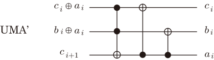
Figure 1: Implementation of UMA’ gate.

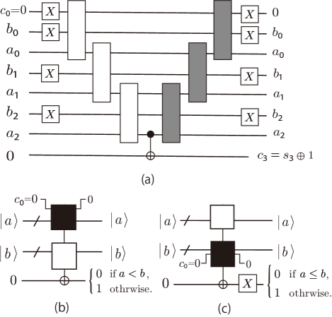
Figure 2: (a): An example of quantum circuit for $n=3$. The white boxes are MAJ gates and the gray boxes are UMA’ gates. (b): (a) is drawn in this way in the main text. This is used when we want to know whether $a<b$ or $a\geq b$. (c): When we want to know whether $a\leq b$ or $a>b$, we use in this way.

Appendix B Addition Circuit

Here we explain the addition circuit of Ref. addition . Let $a=\sum_{j=0}^{r-1}2^{j}a_{j}$ and $b=\sum_{j=0}^{r-1}2^{j}b_{j}$ be two non-negative integers, where $(a_{0},...,a_{r-1})\in\{0,1\}^{r}$ and $(b_{0},...,b_{r-1})\in\{0,1\}^{r}$. Let us define the MAJ gate and the UMA gate as is shown in Fig. 3. Here, $c_{0}=0$ and

$$c_{i+1}=MAJ(a_{i},b_{i},c_{i})=a_{i}b_{i}\oplus b_{i}c_{i}\oplus c_{i}a_{i}$$

for $i\geq 0$, and $s_{i}=a_{i}\oplus b_{i}\oplus c_{i}$ for all $i<r$ and $s_{r}=c_{r}$. The sum of $a$ and $b$ is $a+b=\sum_{j=0}^{r}2^{j}s_{j}$, where $(s_{0},...,s_{r})\in\{0,1\}^{r+1}$. This circuit uses $2n$ TOFFOLI gates and $4n+1$ $CX$-gates.

Figure 3: The MAJ gate and the UMA gate.

In Fig. 4, we provide an example of the addition circuit for $r=3$.

Figure 4: An example of the addition circuit for $r=3$. White boxes are MAJ gates, and black boxes are UMA gates.

- (1) P. W. Shor, Algorithms for quantum computation: discrete logarithms and factoring. Proceedings of the 35th Annual Symposium on Foundations of Computer Science (FOCS 1994), p.124 (1994).
- (2) E. Tang, A quantum-inspired classical algorithm for recommendation systems. Proceedings of the 51st Annual ACM SIGACT Symposium on Theory of Computing (STOC 2019) Pages 217-228.
- (3) L. K. Grover, Quantum mechanics helps in searching for a needle in haystack. Phys. Rev. Lett. 79, 325 (1997).
- (4) B. M. Terhal and D. P. DiVincenzo, Adaptive quantum computation, constant depth quantum circuits and Arthur-Merlin games. Quant. Inf. Comput. 4, 134 (2004).
- (5) S. Aaronson and A. Arkhipov, The computational complexity of linear optics. Theory of Computing 9, 143 (2013).
- (6) M. J. Bremner, R. Jozsa, and D. J. Shepherd, Classical simulation of commuting quantum computations implies collapse of the polynomial hierarchy. Proc. R. Soc. A 467, 459 (2011).
- (7) M. J. Bremner, A. Montanaro, and D. J. Shepherd, Average-case complexity versus approximate simulation of commuting quantum computations, Phys. Rev. Lett. 117, 080501 (2016).
- (8) E. Knill and R. Laflamme, Power of one bit of quantum information. Phys. Rev. Lett. 81, 5672 (1998).
- (9) T. Morimae, K. Fujii, and J. F. Fitzsimons, Hardness of classically simulating the one clean qubit model. Phys. Rev. Lett. 112, 130502 (2014).
- (10) K. Fujii, H. Kobayashi, T. Morimae, H. Nishimura, S. Tamate, and S. Tani, Power of quantum computation with few clean qubits. ICALP 2016.
- (11) K. Fujii, H. Kobayashi, T. Morimae, H. Nishimura, S. Tamate, and S. Tani, Impossibility of classically simulating one-clean-qubit model with multiplicative error. Phys. Rev. Lett. 120, 200502 (2018).
- (12) A. Bouland, B. Fefferman, C. Nirkhe, and U. Vazirani, On the complexity and verification of quantum random circuit sampling. Nat. Phys. 15, pages159–163 (2019).
- (13) R. Movassagh, Efficient unitary paths and quantum computational supremacy: A proof of average-case hardness of Random Circuit Sampling. arXiv:1810.04681
- (14) R. Movassagh, Cayley path and quantum computational supremacy: A proof of average-case -hardness of Random Circuit Sampling with quantified robustness. arXiv:1909.06210
- (15) T. Morimae, Y. Takeuchi, and H. Nishimura, Merlin-Arthur with efficient quantum Merlin and quantum supremacy for the second level of the Fourier hierarchy. Quantum 2, 106 (2018).
- (16) C. Huang, M. Newman, and M. Szegedy, Explicit lower bounds on strong quantum simulation. arXiv:1804.10368
- (17) C. Huang, M. Newman, and M. Szegedy, Explicit lower bounds on strong simulation of quantum circuits in terms of -gate count. arXiv:1902.04764
- (18) R. Impagliazzo and R. Paturi, On the complexity of -SAT. Journal of Computer and System Sciences 62, 367 (2001).
- (19) R. Impagliazzo, R. Paturi, and F. Zane, Which problems have strong exponential complexity? Journal of Computer and System Sciences 63, 512 (2001).
- (20) C. Calabro, R. Impagliazzo, and R. Paturi, The Complexity of Satisfiability of Small Depth Circuits. In: Chen J., Fomin F.V. (eds) Parameterized and Exact Computation. IWPEC 2009. Lecture Notes in Computer Science, vol 5917. Springer, Berlin, Heidelberg.
- (21) A. M. Dalzell, A. W. Harrow, D. E. Koh, and R. L. La Placa, How many qubits are needed for quantum computational supremacy? arXiv:1805.05224
- (22) A. M. Dalzell, Lower bounds on the classical simulation of quantum circuits for quantum supremacy. Bachelor’s thesis, Massachusetts Institute of Technology, 2017.
- (23) E. Farhi and A. W. Harrow, Quantum supremacy through the quantum approximate optimization algorithm, arXiv:1602.07674v1.
- (24) T. Morimae and S. Tamaki, Fine-grained quantum computational supremacy. Quant. Inf. Comput. 19, 1089-1115 (2019).
- (25) R. Williams, A new algorithm for optimal 2-constraint satisfaction and its implications. Ther. Comput. Sci. 348, 357-365 (2005).
- (26) A. Gajentaan and M. H. Overmars, On a class of problems in computational geometry. Computational Geometry 5, 165 (1995).
- (27) Virginia Vassilevska Williams, and Ryan Williams, Subcubic Equivalences Between Path, Matrix, and Triangle Problems. Symposium on Foundations of Computer Science (FOCS), 645 (2010).
- (28) V. V. Williams, Hardness of easy problems: Basing hardness on popular conjectures such as the strong exponential time hypothesis (invited talk). In LIPIcs-Leibniz International Proceedings in Informatics., volume 43, 2015.
- (29) V. Giovannetti, S. Lloyd, and L. Maccone, Quantum Random Access Memory. Phys. Rev. Lett. 100, 160501 (2008).
- (30) A. Barenco et al., Elementary gates for quantum computation. Phys. Rev. A 52, 3457 (1995).
- (31) S. A. Cuccaro, T. G. Draper, S. A. Kutin, and D. P. Moulton, A new quantum ripple-carry addition circuit. arXiv:0410184
- (32) M. Ball, A. Rosen, M. Sabin, and P. N. Vasudevan, Average-case fine-grained hardness, Proceedings of the 49th Annual ACM SIGACT Symposium on Theory of Computing Pages 483-496 (2017).