Deep Reinforcement Learning for Quantum Gate Control

Abstract

How to implement multi-qubit gates efficiently with high precision is essential for realizing universal fault tolerant computing. For a physical system with some external controllable parameters, it is a great challenge to control the time dependence of these parameters to achieve a target multi-qubit gate efficiently and precisely. Here we construct a dueling double deep Q-learning neural network (DDDQN) to find out the optimized time dependence of controllable parameters to implement two typical quantum gates: a single-qubit Hadamard gate and a two-qubit CNOT gate. Compared with traditional optimal control methods, this deep reinforcement learning method can realize efficient and precise gate control without requiring any gradient information during the learning process. This work attempts to pave the way to investigate more quantum control problems with deep reinforcement learning techniques.

I Introduction

High fidelity quantum gate plays an essential role in achieving quantum supremacy Harrow and Montanaro (2017) and fault-tolerant quantum computing PRESKILL (1998). In present days, the study of quantum control has developed a series of methods in practice, such as nuclear magnetic resonance experiments Vandersypen and Chuang (2005), trapped ions Islam et al. (2011); Jurcevic et al. (2014), superconducting qubits Barends et al. (2016), and nitrogen vacancy centers Zhou et al. (2016). Further, based on gradient or evolutionary algorithms, the development of control algorithms provides robust control strategies and have been intensively used. However, it is hard to get such high-quality gates under limited control resources with a precise choice of the control signal, like time-discretization of the fields or fixed amplitude. In a previous work Larocca et al. (2018), under certain limitations, the quantum control landscape was non-convex but will get dumped in the vicinity of quantum speed limit time. Even though the result of the topology of quantum control landscapes has been intensively tested and studied Nielsen et al. (2006); Wu et al. (2012); Nanduri et al. (2013), it is hard to minimize errors of some quantum systems. In addition, these problems can be generalized to hard quantum control problems Zahedinejad et al. (2014). All these limitations are hard to be solved with common quantum-control techniques but meaningful for being discussed in the physical world.

On the other hand, machine learning, already explored as a tool in many aspects of physics Hezaveh et al. (2017); Biamonte et al. (2017), provides a complete paradigm to achieve analysis of various quantum systems  Biamonte et al. (2017); Carleo and Troyer (2017); Carrasquilla and Melko (2017); van Nieuwenburg et al. (2017). With tremendous aspects studied in ML, reinforcement learning (RL) has been a focus on the study of artificial intelligence agent to interact with the real world. Equipped with deep neural network, the deep RL techniques has revolutionized traditional optimal control which provides efficient, precise, and robust performance. Further empowered by advanced optimization techniques, the artificial intelligence agent is able to solve high-dimensional optimization problems such as video games and go Mnih et al. (2015); Silver et al. (2016, 2017). Recently, researchers have begun to utilize some RL algorithms in the quantum control studies Bukov et al. (2018); Niu et al. (2018). The novel RL algorithm provides advanced optimization techniques which are able to solve more difficult optimization problems.

In this article, we investigate the traditional quantum gate control problem where an efficient strategy for preparing high fidelity quantum gate proposed by an artificial intelligence agent. With deep RL, we propose a framework to connect optimal decision making of the underlying quantum dynamics with state-of-the-art RL techniques. In particular, within the present framework, the agent performs optimal discrete, sequential controls to get two typical quantum gates: a single-qubit Hadamard gate and a two-qubit CNOT gate. The results provide a general way to investigating the quantum control problem with deep RL techniques.

The rest of this paper is structured as follows. In Sec.II, we briefly overview our quantum gate control model. In Sec.III, we present some relative RL algorithms and the DDDQN method for two quantum gate control models. In Sec. IV and V, we show the numerical results and draw our conclusions.

II Bang-bang control model to implement quantum gates

In this section, we give a bang-bang control model to implement quantum gates, which explains the physical problems we solve in this paper.

We consider a quantum system whose Hamiltonian is

$$H(\vec{\epsilon}(t))={H}_{d}+{H}_{c}(\vec{\epsilon}(t)),$$ (1)

where the term ${H}_{d}$, called the drifted Hamiltonian, is the free evolution part of the Hamiltonian ${H}(\vec{\epsilon}(t))$. Another part of the Hamiltonian, ${H}_{c}(\vec{\epsilon}(t))$, called the control Hamiltonian, is under control by some time dependent external parameter vector $\vec{\epsilon}(t)$.

In our bang-bang control protocol, our total control time $T$ is fixed, which is divided into $N$ short time periods with the same duration $\delta t=T/N$. In the $i$-th time period with $(i-1)\delta t\leq t\leq i\delta t$ ($1\leq i\leq N$), the control parameter vector is constant, i.e. $\vec{\epsilon}(t)=\vec{\epsilon}_{i}$, where the control parameter vector $\vec{\epsilon}_{i}$ are selected from a set $\mathcal{A}(\vec{\epsilon})$ of $d$ possible choices. The unitary evolution operator in the $i$-th time period is

$$U(i\delta t,(i-1)\delta t;\vec{\epsilon}_{i})=e^{-iH(\vec{\epsilon}_{i})\delta t}.$$ (2)

When all the $N$ control parameter vectors $\{\vec{\epsilon}_{1},\vec{\epsilon}_{2},\ldots,\vec{\epsilon}_{N}\}$ are selected, the unitary operator at time $T$ is determined by the iterative equations

$$U(i\delta t) =U(i\delta t,(i-1)\delta t;\vec{\epsilon}_{i})U((i-1)\delta t),$$ (3)

$$U(0) =I,$$ (4)

where $I$ is the identity operator in the Hilbert space of our system.

Our aim is to select the parameter vectors $\{\vec{\epsilon}_{1},\vec{\epsilon}_{2},\ldots,\vec{\epsilon}_{N}\}$ to make the unitary operator $U(T)$ approximate the target unitary gate $U_{f}$ as well as possible, which is formulated by maximizing the fidelity

$$\mathcal{F}(T)=\max_{\vec{\epsilon}_{1},\vec{\epsilon}_{2},\ldots,\vec{\epsilon}_{N}}\mathcal{F}(T;\vec{\epsilon}_{1},\vec{\epsilon}_{2},\ldots,\vec{\epsilon}_{N})$$ (5)

with the fidelity

$$\mathcal{F}(T;\vec{\epsilon}_{1},\vec{\epsilon}_{2},\ldots,\vec{\epsilon}_{N})=\left|\frac{\mathrm{Tr}\{{U}_{f}^{\dagger}{U}(T)\}}{D}\right|^{2},$$ (6)

where $D$ is the dimension of the Hilbert space. We observe that $\mathcal{F}(T;\vec{\epsilon}_{1},\vec{\epsilon}_{2},\ldots,\vec{\epsilon}_{N})\in[0,1]$, and that $\mathcal{F}(T;\vec{\epsilon}_{1},\vec{\epsilon}_{2},\ldots,\vec{\epsilon}_{N})=1$ if and only if ${U}(T)$ is equal to ${U}_{f}$ up to a phase factor.

In particular, the size of the set of the parameter vectors is $d^{N}$, which implies that it is impossible to exhaustively searching the optimal parameter vector sequence for a large $N$.

Here we focus on two typical target quantum gates, one is the Hadmard gate, the other is the CNOT gate.

II.1 Hadamard gate

When the target quantum gate is the single qubit Hadmard gate

$$U_{f}=\frac{1}{\sqrt{2}}\begin{pmatrix}1&1\\ 1&-1\end{pmatrix},$$ (7)

we consider a two-level system whose Hamiltonian is

$$H(\epsilon(t))=\sigma_{z}+\epsilon(t)\sigma_{x},$$ (8)

where $\sigma_{z}$ and $\sigma_{x}$ are Pauli matrices, and $\epsilon(t)$ is a real control parameter. This simple model has been widely applied in quantum physics, e.g., it describes the non-adiabatic transition Zener (1932), the Landau-Zener-Stuckelberg interferometry Shevchenko et al. (2010) and the Kibble-Zurek mechanism Zurek et al. (2005).

Based on the Pontryagin maximum principle, we take the set of $d=2$ possible control parameter $\mathcal{A}(\epsilon)\in\{\pm 4\}$ in our bang-bang protocol.

II.2 CNOT gate

When the target quantum gate is the CNOT gate

$$U_{f}=\begin{pmatrix}1&0&0&0\\ 0&1&0&0\\ 0&0&0&1\\ 0&0&1&0\end{pmatrix},$$ (9)

we consider the Hamiltonian

$$\begin{split}H(\epsilon(t))=&\sigma_{z}^{(1)}\otimes\sigma_{z}^{(2)}+\epsilon_{1}(t)\sigma_{x}^{(1)}\otimes\mathbb{I}^{(2)}+\epsilon_{2}(t)\mathbb{I}^{(1)}\otimes\sigma_{x}^{(2)}\\ &+\epsilon_{3}(t)\sigma_{y}^{(1)}\otimes\mathbb{I}^{(2)}+\epsilon_{4}(t)\mathbb{I}^{(1)}\otimes\sigma_{y}^{(2)},\end{split}$$ (10)

where $\mathbb{I}$ is the $2\times 2$ identity matrix, and $\vec{\epsilon}(t)=(\epsilon_{1}(t),\dots,\epsilon_{4}(t))$ is a $4$ component parameter vector.

Similarly as in the case of the Hadmard gate, we take the set of $d=16$ possible choices of the parameter vector as

$$\mathcal{A}(\vec{\epsilon})=\{(\epsilon_{1},\epsilon_{2},\epsilon_{3},\epsilon_{4})\text{ with }\epsilon_{i}\in\{\pm 4\}\}.$$ (11)

III Deep reinforcement learning methods 

In this section, we show how to apply the deep RL to approximately solve the maximization problem specified by Eq. (5) in our bang-bang control quantum gate implementation protocol. To this end, we firstly review the necessary concepts in deep RL methods, especially the framework of the dueling double deep Q-learning neural network, which is adopted in our problem. Then we show how to combine our bang-bang control protocol with the deep RL methods.

III.1 Reinforcement learning

RL is a kind of ML method in which an intelligent agent aims to find a series of actions on a given environment to optimize its performance by delayed scalar rewards received Sutton and Barto (1998).

The problem of RL is described as a finite Markov decision process Sutton and Barto (1998). At time $t=0$, the state of the environment is $S_{0}$, and the agent chooses an action $A_{0}$. At time $t=1$, the state of the environment becomes $S_{1}$ after the action $A_{0}$, and the environment also gives a scalar reward $R_{1}$. Then the agent chooses an action $A_{1}$, and repeats the above procedure. In general, this Markov process is described as a state-action-reward sequence

$$S_{0},A_{0},R_{1},S_{1},A_{1},R_{2},\dots$$

For a finite Markov decision process, the sets of the states, the actions and the rewards are finite. The total discounted return at time $t$

$$G_{t}=\sum_{k=0}^{\infty}\gamma^{k}R_{t+k+1},$$ (12)

where $\gamma$ is the discount rate and $0\leq\gamma\leq 1$.

In RL, the agent selects the actions according to a policy $\pi$, which is specified by a conditional probability of selecting an action $A$ for each state $S$, denoted as $\pi(A|S)$. The task of the agent is to learn an optimal policy $\pi_{\ast}$, which maximizes the expected discounted return

$$V_{\pi}(s)=E_{\pi}(G_{t}|S_{t}=s),$$ (13)

where $E_{\pi}$ denotes the average expectation under the policy $\pi$.

It has been shown that the optimal policy $\pi^{*}$ exists and can be found iteratively as follows. Let us introduce the value of state-action function, the conditional discount return

$$Q_{\pi}(s,a)=E_{\pi}(G_{t}|S_{t}=s,A_{t}=a).$$ (14)

If we have a policy $\pi$, then we calculate the value of state-action function $Q_{\pi}(S,A)$. For each state $s$, we take an action maximizing the value of state action $Q_{\pi}(s,A)$, which forms our new policy $\pi^{\prime}$. Then we calculate the value of state-action function $Q_{\pi^{\prime}}(S,A)$. Repeating the above procedure until the new policy equals the updated one, which is the optimal policy $\pi^{*}$ we are looking for.

Another well known method to get the optimal policy $\pi^{\ast}$ is the Q-learning Watkins (1989), an off-policy temporal-difference control algorithm defined as

$$Q(S_{t},A_{t})\leftarrow Q(S_{t},A_{t})+\Delta Q$$ (15)

with

$$\Delta Q=\alpha[R_{t+1}+\gamma\max_{a}Q(S_{t+1},a)-Q(S_{t},A_{t})],$$ (16)

where $\alpha$ is the step size parameter.

III.2 Dueling Double Deep Q-learning

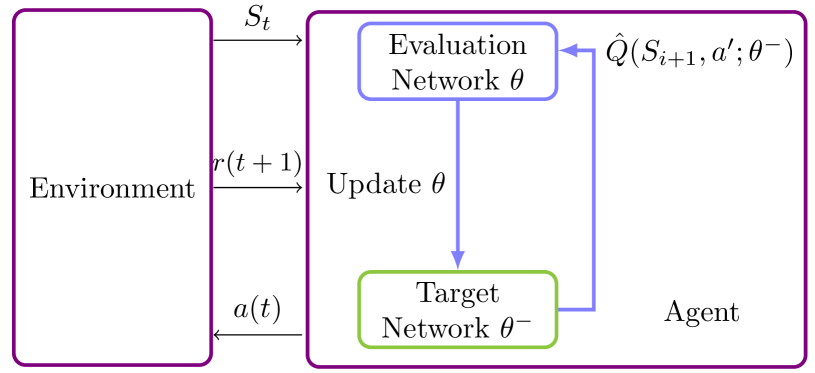
Figure 1: An overview of the deep RL: at each time step of training, the evaluation network of the agent proposes a control action of $a(t)$, the environment takes the proposed action and evaluates gate of Eq. (2) for time duration $\delta t$ to obtain a new unitary gate $U_{t+1}$ and calculates the reward of Eq. (21) , both of which are fed into the RL agent. The evaluation network of the agent is updated with the loss function of Eq. (17) by backpropagation. With fixed numbers of steps, the agent updates the parameters of the target network by transferring the parameters of evaluation network.

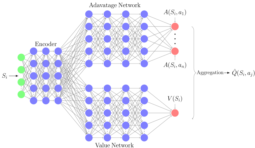
Figure 2: The deep neural network architecture of our agent: For each state fed into the neural network, the encoder extracts the information of the state for further calculation. The value network and advantage network get the information of the encoder to calculate the value of the state for each action. Based on Eq. (18), the neural network aggregates the value of the state and the advantage of action by the state to get the state-action values $\hat{Q}(S_{i},a_{j})$.

In this section, we introduce the Dueling Double Deep Q-learning Neural Network (DDDQN), which will be used in our quantum gate control problem. The advantage of this method has been discussed in previous research Wang et al. (2015).

First, we begin by introducing the double Q-learning method Hasselt (2010) in the training of our agent. As shown in Fig. 2, the agent consists of the evaluation network and the target network with the same architecture. The evaluation network evaluates the state-action value ${Q}(S,A;\theta)$, and the target network evaluates the TD target ${Q}(S,A;\theta^{-})$. At each learning step, we fed the agent with a minibatch of experiences $\{S_{t},A_{t},R_{t+1},S_{t+1}\}$ with the prioritized experience replay (PER) method Schaul et al. (2016). The state $S_{t}$ is fed into the evaluation network to calculate the state-action value ${Q}(S_{t},A_{t};\theta)$. At the same time, the target network is to calculate $\max\limits_{a^{\prime}}{Q}(S_{t+1},a^{\prime};\theta^{-})$ in Eq. (17). At the end of each step of training, the evaluation network is updated through the back-propagation by minimizing the loss. Based on Eq. (15), the loss is the mean square error (MSE) of the difference between the evaluation ${Q}(S_{t},A_{t};\theta)$ and the target $\max\limits_{a^{\prime}}{Q}(S_{t+1},a^{\prime};\theta^{-})$

$$\rm{loss}=\rm{MSE}((R_{t+1}+\gamma\max\limits_{a^{\prime}}{{Q}}(S_{t+1},a^{\prime};\theta^{-}))-{Q}(S_{t},A_{t};\theta)).$$ (17)

During the learning episodes (see Fig. 2), the agent updates the parameters of the target network $\theta^{-}\rightarrow\theta$ to make better decisions.

Further, the detailed architecture of each network in our agent is shown in Fig. 2. Each network is consisted of three parts: an encoder, an advantage network and a value network. The encoder extracts information about the states $S_{t}$ for the next two neural networks. Based on the Q-learning, the state-action value ${Q}(S_{t},A_{t})$ represents the expected return for the agent to select the action $A_{t}$ on the state $S_{t}$ of the environment. In the architecture of the dueling network Wang et al. (2015) in deep RL, we decompose the state-action value as

$$Q(S_{t},A_{t})=A(S_{t},A_{t})+V(S_{t}),$$ (18)

where $V(S_{t})$ is the state value for each state, and $A(S_{t},A_{t})$ is the advantage for each action. The state value $V(S_{t})$ is calculated by the advantage network, and the advantage of action $A(S_{t},A_{t})$ is calculated by the value network. Then we combine these two values to get an estimate of $Q(S_{t},A_{t})$ through an aggregation layer.

III.3 Quantum gate control with DDDQN

To apply the reinforcement ML to our bang-bang control protocol, we need to build a map between their concepts. The state of the environment at time $t$ is

$$\begin{split}S_{t}=U(t\delta t)=\{\Re(U_{ij}(t\delta t)),\Im(U_{ij}(t\delta t))\},\end{split}$$ (19)

where $U_{ij}(t\delta t)$ is the matrix element of $U(t\delta t)$, and $\Re,\Im$ mean taking the real part and the imaginary part. The action the agent at time $t$ can take

$$a(\vec{\epsilon})=U(t\delta t,(t-1)\delta t;\vec{\epsilon}).$$ (20)

Note that the action does not depend on time $t$. The reward of the agent received in each step is

$$R_{t}=\begin{cases}0,&t\in\{0,1,\dots,N-1\}\\ -\mathcal{L}(\mathcal{F}(T;\vec{\epsilon}_{1},\vec{\epsilon}_{1},\ldots,\vec{\epsilon}_{N})),&t=N\end{cases}$$ (21)

where $\mathcal{L}(\mathcal{F})$ is the logarithmic infidelity, $\mathcal{L}(\mathcal{F})=\log_{10}(1-\mathcal{F})$. In other words, the agent will not get a reward immediately, but at time $N$.

Our algorithm for quantum gate control with DDDQN is given in Algorithm 1.

Initialize memory R to empty;

Randomly initialize the evaluation network with random weights $\theta$;

Randomly initialize the target network with random weights $\theta^{-}$;

for episode= 0, M do

      Initialize $s_{0}$ , $s_{0}=f(U_{0})$;

      

      for $t=0,\dots,t_{N}$ do

            With probability $\epsilon$ select a random action $a_{t}$, otherwise $a_{t}=argmax_{a}{Q}(s_{t},a;\theta)$;

            

            Execute action $a_{t}$ and observe the reward $r_{t+1}$, and the next state $s_{t+1}$;

            

            Store experience $e_{t}=(s_{t};a_{t};r_{t+1};s_{t+1})$ in R;

            

            if $t=t_{N}$ then

                   Sample minibatch of experiences $e_{i}$ with PER method;

                  

                  Set $y_{i}=\left\{\begin{array}[]{lc}r_{i+1}&\text{if $t_{i+1}=t_{N}$ }\\ r_{i+1}+\gamma\mathop{\arg\max}_{a^{\prime}}{Q}(s_{t+1},a^{\prime};\theta^{-})&\text{otherwise}\end{array}\right.$ 

                  Update $\theta$ by minimizing $\text{loss}=(y_{i}-{Q}(s_{t},a_{i};\theta))^{2}$;

                  

             end if

             Every C times of learning, set $\theta^{-}=\theta$;

            

       end for

       

end for

 

Algorithm 1 Deep RL for quantum gate control

IV Numerical results

In this section, we give the numerical results of the logarithmic infidelity $\mathcal{L}$ with target gates being the single-qubit Hadamard gate and the two-qubit CNOT gate from the deep reinforcement learning. To show the effectiveness of our deep RL method, we also calculate the logarithmic infidelity with three different algorithms: gradient ascent pulse engineering (GRAPE), differential evolution (DE), and genetic algorithm (GA). We then present our analysis of the performance of our deep RL algorithm against the other three algorithms.

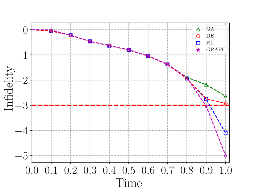
Figure 3: Best infidelities of preparing a single-qubit Hadamard gate in different evolution time T. The markers correspond to the algorithms RL (blue $\Box$), GRAPE(purple ✩), DE(red $\circ$) and GA (green $\triangle$). The time step $N=28$ for different $T$. Here we set 400 iterations for GRAPE DE and GA, 100000 training episodes for RL.

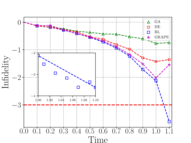
Figure 4: Best infidelities of preparing a CNOT gate in different evolution time T. The markers correspond to the algorithms RL (blue $\Box$), GRAPE(purple ✩), DE(red $\circ$) and GA (green $\triangle$). The time step $N=38$ for different $T$. Here we set 5000 iterations for GRAPE DE and GA, 150000 training episodes for RL.

Fig. 3 shows the minimal logarithmic infidelities of preparing a single-qubit Hadmard gate in different evolution time $T$ with different algorithms. For $T<0.8$, the results on the infidelities from the four algorithms agree well. At $T=0.9$, the results on the logarithmic from RL and DE agree well, which is better than that from GA, and worse than that from GRAPE. At $T=1.0$, the infidelity obtained from RL and GRAPE abruptly decrease, which possibly implies that the speed limit time of the problem is in the region $[0.9,1.0]$. In particular, these two algorithms find protocols to achieve infidelity $\mathcal{L}<-3$ (red line) or fidelity $\mathcal{F}>99.9\%$ at $T=1.0$. While GRAPE has the best performance out of the four methods, the algorithm requires the fidelity gradients at all time, and it is not readily accessible through experimental measurements. Further, GRAPE allows for the control field $\epsilon(t)$ to take any value in the interval $[-4,4]$.

In Fig. 4, we compare the results of the CNOT gate control task from the four algorithms. Similar as in the previous task, all the algorithms perform well for $T<0.4$. RL, DE and GRAPE find optimal protocols in the time region $0.4<T<0.9$, but the performance of GA is poor for $T>0.4$. After $T=0.9$, only RL and GRAPE find optimal protocols, and the results of our RL agent are better than that of the GRAPE. Notice that at $T=1.1$, the landscape seems to get dumped for the problem and all the algorithms except RL get trapped. Like the state transfer problem  Alexandrec; Bukov et al. (2018), we believe this region may have a similar phase transition phenomenon and traditional algorithms are hard to maintain good performance. However, our RL agent ignores the dumped landscape and finds good protocols compared with other algorithms. To investigate the performance of RL in this region, we plot detailed results in the inset of Fig. 4. The results show that the agent has good and robust performance in the region.

V CONCLUSION

In this article, we apply the deep RL to explore the fast and high-precision quantum gate control problem. The quantum gate control problem is then mapped into a deep RL algorithm. Further, we build an RL agent to solve the quantum optimal control problem. We compare the numerical results among the four different algorithms on two typical quantum gate control problems. Our results demonstrate that the artificial intelligent is able to effectively learn the optimal control schemes in approximating the target quantum gates. The success of our agent lies in its suitability for solving discrete action problems and its state of art RL technique of balancing explore and exploit.

The numerical results show that the performance of deep RL is robust and efficient in implementing arbitrary single and two qubit gates. However, there are still some challenges to extend RL algorithms to multi-qubit control problem. The main challenge needs to solve is that the control space will grow exponentially with the increase of qubit number. We hope that our approach can inspire more applications of deep RL methods in the quantum control domain.

Appendix A Hyper-Parameters and Learning Curves

Our RL agent makes use of a deep neural network to approximate the Q values for the possible actions of each state. The network (see Fig. 2) consists of 4 layers of each sub-network. All layers have ReLU activation functions except the output layer which has linear activation. The hyper-parameters of the network are summarized in Table LABEL:para. As shown in Fig. 5, the learning result highly depends on the layer number of neural network. The computational time is summarized in Table LABEL:time. Notice that the training time of two-qubit gate is from $6$ to $30$ times larger than that of one qubit gate. Among all algorithms discussed in the paper, the resources needed by our RL agent increase slowest. The learning curves for the two quantum gates are shown in Fig. 6 and Fig. 7. All algorithms are implemented with Python 3.6, and have been run on two 14-core 2.60GHz CPU with 188 GB memory and four GPUs.

Table 1: Training Hyper-Parameters

Hyper-parameter	Values
Neurons in decoder network	$\{600,600,600\}$
Neurons in advantage(value) network	$\{600,600,600,600\}$
Minibatch size	a
Replay memory size	100000
Learning rate	$0.001$b
Update period	100
Reward decay $\gamma$	0.95
Total episode	c

• 72 for Hadamard gate problem, 128 for CNOT gate problem

• With Adam algorithm

• 50000 for Hadamard gate problem, 150000 for CNOT gate problem

Table 2: Training time of different algorithms

Algorithm	Time
	Hadamard gate	CNOT gate
GRAPE	$<20s$	about 7 min
GA	about 20 min	about 10 h
DE	about 40 min	about 18 h
RL	about 5 h	about 31 h

• The computation iterations is same with Fig 3 and Fig 4

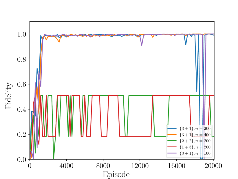
Figure 5: Learning curves of RL agent for Hadamard gate at $T=1$ with different neural network architectures. With different layer numbers $\{\textrm{encoder network + Advantage (Value) network}\}$ and neuron numbers $n$ of each architecture.

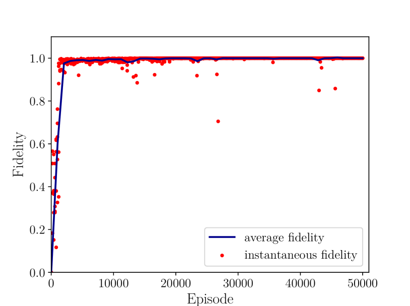
Figure 6: Learning curves of the RL agent for Hadamard gate at $T=1$. The red dots show the instantaneous fidelity at every episode with 5 times, while the blue line the average fidelity of the 5 agent.

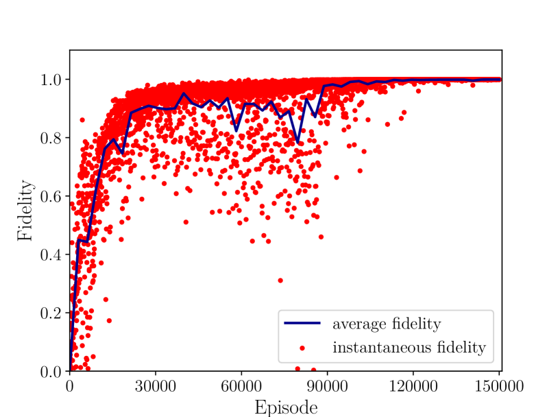
Figure 7: Learning curves of the RL agent for CNOT gate at $T=1.1$. The red dots show the instantaneous fidelity at every episode with 5 times, while the blue line the average fidelity of the 5 agent.

References

- Harrow and Montanaro (2017) A. W. Harrowand A. Montanaro, Nature 549, 203 (2017).
- PRESKILL (1998) J. PRESKILL, in Introduction to Quantum Computation and Information (WORLD SCIENTIFIC, 1998) pp. 213–269.
- Vandersypen and Chuang (2005) L. M. K. Vandersypenand I. L. Chuang, Rev. Mod. Phys. 76, 1037 (2005).
- Islam et al. (2011) R. Islam, E. E. Edwards, and a. o. Kim, Nat. Commun. 2, 377 (2011).
- Jurcevic et al. (2014) P. Jurcevic, B. P. Lanyon, Hauke, et al., Nature 511, 202 (2014).
- Barends et al. (2016) R. Barends, A. Shabani, Lamata, et al., Nature 534, 222 (2016).
- Zhou et al. (2016) B. Zhou, A. Baksic, Ribeiro, et al., Nat. Phys. 13, 330 (2016).
- Larocca et al. (2018) M. Larocca, P. Poggi, and D. Wisniacki, (2018), arXiv:1802.05683 .
- Nielsen et al. (2006) M. A. Nielsen, M. R. Dowling, M. Gu, and A. C. Doherty, Phys. Rev. A 73, 062323 (2006).
- Wu et al. (2012) R.-B. Wu, R. Long, J. Dominy, et al., Phys. Rev. A 86, 013405 (2012).
- Nanduri et al. (2013) A. Nanduri, A. Donovan, T.-S. Ho, and H. Rabitz, Phys. Rev. A 88, 033425 (2013).
- Zahedinejad et al. (2014) E. Zahedinejad, S. Schirmer, and B. C. Sanders, Phys. Rev. A 90, 032310 (2014).
- Hezaveh et al. (2017) Y. D. Hezaveh, L. P. Levasseur, and P. J. Marshall, Nature 548, 555 (2017).
- Biamonte et al. (2017) J. Biamonte, P. Wittek, N. Pancotti, P. Rebentrost, N. Wiebe, and S. Lloyd, Nature 549, 195 (2017).
- Carleo and Troyer (2017) G. Carleoand M. Troyer, Science (New York, N.Y.) 355, 602—606 (2017).
- Carrasquilla and Melko (2017) J. Carrasquillaand R. G. Melko, Nature Physics 13, 431 (2017).
- van Nieuwenburg et al. (2017) E. van Nieuwenburg, Y.-H. Liu, and S. Huber, Nature Physics 13, 435 (2017).
- Mnih et al. (2015) V. Mnih, K. Kavukcuoglu, D. Silver, et al., Nature 518, 529 (2015).
- Silver et al. (2016) D. Silver, A. Huang, C. J. Maddison, et al., Nature 529, 484 (2016).
- Silver et al. (2017) D. Silver, J. Schrittwieser, K. Simonyan, et al., Nature 550, 354 (2017).
- Bukov et al. (2018) M. Bukov, A. G. R. Day, D. Sels, P. Weinberg, A. Polkovnikov, and P. Mehta, Phys. Rev. X 8, 031086 (2018).
- Niu et al. (2018) M. Y. Niu, S. Boixo, V. Smelyanskiy, and H. Neven, (2018), arXiv:1803.01857 .
- Zener (1932) C. Zener, Proceedings of the Royal Society of London A: Mathematical, Physical and Engineering Sciences 137, 696 (1932).
- Shevchenko et al. (2010) S. Shevchenko, S. Ashhab, and F. Nori, Physics Reports 492, 1 (2010).
- Zurek et al. (2005) W. H. Zurek, U. Dorner, and P. Zoller, Phys. Rev. Lett. 95, 105701 (2005).
- Sutton and Barto (1998) R. S. Suttonand A. G. Barto, Reinforcement Learning: An Introduction (MIT Press, 1998).
- Watkins (1989) C. Watkins, Learning From Delayed Rewards, Ph.D. thesis, Cambridge University Psychology Department (1989).
- Wang et al. (2015) Z. Wang, N. de Freitas, and M. Lanctot, (2015), arXiv:1511.06581 .
- Hasselt (2010) H. V. Hasselt, in Advances in Neural Information Processing Systems 23, edited by J. D. Lafferty, C. K. I. Williams, J. Shawe-Taylor, R. S. Zemel, and A. Culotta (Curran Associates, Inc., 2010) pp. 2613–2621.
- Schaul et al. (2016) T. Schaul, J. Quan, I. Antonoglou, and D. Silver, CoRR abs/1511.05952 (2016).
- Day et al. (2019) A. G. R. Day, M. Bukov, P. Weinberg, P. Mehta, and D. Sels, Phys. Rev. Lett. 122, 020601 (2019).