Charge nonconservation of molecular devices in the presence of a nonlocal potential

Abstract

In the presence of a nonlocal potential in molecular device systems, generally the charge conservation cannot be satisfied, and in literatures the modifications of the conventional definition of current were given to solve this problem. We demonstrate that, however, the nonconservation is not due to the invalidation of the conventional definition of current, but originates respectively from the improper approximations to electron-electron interactions and the inappropriate definition of current using pseudo wave functions in pseudopotential implementations. In this work, we propose a nonlocal-potential formulation of the interactions to fulfill the charge conservation and also give a discussion about the calculation of current when the pseudopotential is involved. As an example of application of our formulation, we further present the calculated results of a double-barrier model.

I Introduction

Over the past few decades, investigations on transport properties of mesoscopic systems and nanostructures have been extensively reported both on experimental advances1 ; 2 ; 3 ; 4 ; 5 ; 6 ; 7 ; 8 ; 9 ; 10 ; 11 ; 12 ; 13 and theoretical explorations.14 ; 15 ; 16 ; 17 ; 18 ; 19 ; 20 ; 21 ; 22 ; 23 ; 24 ; 25 ; 26 ; 27 It is widely acknowledged that these functional devices can be constituted by ultrasmall conjugated molecules, single-layer or multi-layer nanotubes, bulk organic molecules, etc., and plenty of interesting phenomena such as molecular field effects,1 Coulomb blockade,2 negative differential resistance3 and conductance switching effects4 have been revealed, which exhibit fundamental significance and potential microelectronic applications. In most of the works, considerable research efforts are focused on current-voltage ($I$-$V$) characteristics as the $I$-$V$ profiles provide opportunities for a deeper understanding of, e.g., the basic mechanism and structure properties, as well as promising guidance for future molecular nanoelectronics designs and manipulations.

On the theoretical side, calculations for the $I$-$V$ characteristics of molecular device systems are mostly performed by employing the self-consistent field (SCF) theory or nonequilibrium Green’s functions combined with density functional theory (NEGF-DFT),18 ; 19 ; 20 and the widely used DFT calculations at present can be vested in the SCF method. In comparison with conventional SCF,28 ; 29 ; 30 in addition to self-consistent Hartree potential DFT introduces the exchange-correlation potential, which is nonlocal if one wants to go beyond the local density approximation.31 It has been shown that if the Hamiltonian $H$ includes a general nonlocal potential $V(\mathbf{r},\mathbf{r}^{\prime})$, an extra term naturally appears in the continuity equation and the charge conservation will not be fulfilled.24 ; 25 ; 32 ; 33 Thus the calculations may give very incorrect results, even nonphysical results.

To resolve the problem, Li et al.32 proposed a scheme to modify the conventional definition of current density to include the additional current induced by the nonlocal potential $V(\mathbf{r},\mathbf{r}^{\prime})$, and therefore yield the charge conservation in a computationally efficacious way. However, either local or nonlocal exchange-correlation potential stems from the approximation to electron-electron interactions, and according to the conventional definition of current density we will demonstrate fundamentally that with the Hamiltonian including the exact electron-electron interactions the extra term does not appear and the conservation can be precisely satisfied. Hence the problem of charge nonconservation coming from the nonlocal exchange-correlation potential should not be settled by redefining the current density. Instead, it has to be resolved by finding a reasonable nonlocal-potential approximation to the electron-electron interactions to eliminate the extra term. On the other hand, norm-conserving pseudopotentials 34 are generally utilized to reduce the size of plane-wave basis sets in first-principles calculations, which is another origin of the nonlocal potential.35 Nevertheless, the pseudopotential implementations give the pseudo wave functions, while in the continuity equation $\partial_{t}\rho+\nabla\cdot\mathbf{J}=0$ the charge density $\rho$ and the current density $\mathbf{J}$ should be calculated by using the true wave functions instead of the pseudo ones. Therefore, when the pseudopotential method is employed, the extra term appearing in the continuity equation is due to the improper utilization of the pseudo wave functions for calculating the current, and the problem of charge nonconservation coming from the nonlocal pseudopotential should not be resolved by redefining the current density either. From a fundamental point of view, the continuity equation is a criterion regardless of any approximations brought in as long as the particles of the system are conserved, which can be easily proved with the original Hamiltonian. It is the purpose of this work to investigate the above problems.

The paper is organized as follows. In Sec. II, the origins of the nonlocal potential and the consequent issues of charge nonconservation are discussed. We lay special emphasis on the nonlocal exchange-correlation potential from the starting point of second quantization, and subsequently demonstrate that in DFT calculations the nonconservation is caused by the inappropriate definition of current using pseudo wave functions rather than the introduction of the pseudopotentials. As an example, the currents of a double-barrier model are numerically calculated in Sec. III to confirm our theoretical formulation. Section IV gives the conclusions and discussions.

II Theoretical Formulation

In the context of first-principles calculations, if one uses true wave functions $\psi\left(\mathbf{r}\right)$ of the system from the very beginning throughout the processes, the continuity equation $\partial_{t}\rho_{c}+\nabla\cdot\mathbf{J}_{c}=0$ can be easily realized according to the Schördinger equation, where $\rho_{c}=\left|\psi\left(\mathbf{r}\right)\right|^{2}$ is the conventional electron density and $\mathbf{J}_{c}$ is the conventional current density in the absence of magnetic field with the definition as

$$\mathbf{J}_{c}=\frac{-i\hbar}{2m}\left[\psi^{\ast}\left(\mathbf{r}\right)\nabla\psi\left(\mathbf{r}\right)-\psi(\mathbf{r})\nabla\psi^{\ast}(\mathbf{r})\right].$$ (1)

One of the origins of the charge nonconservation comes from the approximation to electron-electron interactions, i.e., some improper exchange-correlation potentials are introduced. We will show that according to the conventional definition of current density, the conservation is still satisfied in the presence of the interactions, but generally can be violated by introducing the nonlocal exchange-correlation potentials. To see this, the simplest case of Hamiltonian of a finite many-electron system is considered, in which the electron-electron interactions are not taken into account firstly so that the second quantized nonrelativistic Hamiltonian (a quantity with a caret symbol denotes an operator) is

$$\hat{H}_{0}=\hat{T}_{s}+\hat{U}_{ex},$$ (2)

where in terms of the field operators $\hat{\Psi}^{{\dagger}}\left(\mathbf{r},t\right)$ and $\hat{\Psi}\left(\mathbf{r},t\right)$, the single-particle kinetic energy operator and the external potential operator can be written respectively as36 ; 37

$$\hat{T}_{s}=\frac{-\hbar^{2}}{2m}\int d\mathbf{r}\hat{\Psi}^{{\dagger}}\left(\mathbf{r},t\right)\nabla^{2}\hat{\Psi}\left(\mathbf{r},t\right),$$ (3)

and

$$\hat{U}_{ex}=\int d\mathbf{r}\hat{\Psi}^{{\dagger}}\left(\mathbf{r},t\right)v\left(\mathbf{r},t\right)\hat{\Psi}\left(\mathbf{r},t\right).$$ (4)

The density operator can be defined as $\hat{n}(\mathbf{r},t)=$ $\hat{\Psi}^{{\dagger}}\left(\mathbf{r},t\right)\hat{\Psi}\left(\mathbf{r},t\right)$ and the current density operator as the conventional form is

$$\hat{\mathbf{J}}_{c}(\mathbf{r},t)=\frac{-i\hbar}{2m}\left[\hat{\Psi}^{{\dagger}}\left(\mathbf{r},t\right)\nabla\hat{\Psi}\left(\mathbf{r},t\right)-\left[\nabla\hat{\Psi}^{{\dagger}}\left(\mathbf{r},t\right)\right]\hat{\Psi}\left(\mathbf{r},t\right)\right],$$ (5)

by means of the Heisenberg’s equation and the anticommutation relation that we obtain

$$\frac{\partial\hat{n}\left(\mathbf{r},t\right)}{\partial t}= \frac{1}{i\hbar}\left[\hat{n}\left(\mathbf{r},t\right),\hat{H}_{0}\right]$$

$$= \frac{i\hbar}{2m}\left[\hat{\Psi}^{{\dagger}}\left(\mathbf{r},t\right)\nabla^{2}\hat{\Psi}\left(\mathbf{r},t\right)\right.$$

$$\text{ \ \ }\left.-\left[\nabla^{2}\hat{\Psi}^{{\dagger}}\left(\mathbf{r},t\right)\right]\hat{\Psi}\left(\mathbf{r},t\right)\right]$$

$$= -\nabla\cdot\hat{\mathbf{J}}_{c}\left(\mathbf{r},t\right),$$ (6)

where the charge conservation is accomplished, as expected. The corresponding Hamiltonian including the interactions can be written as

$$\hat{H}_{w}=\hat{T}_{s}+\hat{U}_{ex}+\hat{W},$$ (7)

where

$$\hat{W}=\int d\mathbf{r}^{\prime\prime}d\mathbf{r}^{\prime}w\left(\left|\mathbf{r}^{\prime}-\mathbf{r}^{\prime\prime}\right|\right)\hat{\Psi}^{{\dagger}}\left(\mathbf{r}^{\prime}\right)\hat{\Psi}^{{\dagger}}\left(\mathbf{r}^{\prime\prime}\right)\hat{\Psi}\left(\mathbf{r}^{\prime\prime}\right)\hat{\Psi}\left(\mathbf{r}^{\prime}\right).$$ (8)

Since the foregoing equations present the continuity with respect to $\hat{T}_{s}$ and $\hat{U}_{ex}$, only interaction operator is taken into account hereafter, i.e.,

$$\left[\hat{n}\left(\mathbf{r},t\right),\hat{W}\right]$$

$$=\left[\hat{\Psi}^{{\dagger}}\left(\mathbf{r},t\right)\hat{\Psi}\left(\mathbf{r},t\right),\right.\int d\mathbf{r}^{\prime\prime}d\mathbf{r}^{\prime}w\left(\left|\mathbf{r}^{\prime}-\mathbf{r}^{\prime\prime}\right|\right)\hat{\Psi}^{{\dagger}}\left(\mathbf{r}^{\prime},t\right)$$

$$\text{ \ \ }\left.\times\hat{\Psi}^{{\dagger}}\left(\mathbf{r}^{\prime\prime},t\right)\hat{\Psi}\left(\mathbf{r}^{\prime\prime},t\right)\hat{\Psi}\left(\mathbf{r}^{\prime},t\right)\right]$$

$$=\int d\mathbf{r}^{\prime\prime}d\mathbf{r}^{\prime}w\left(\left|\mathbf{r}^{\prime}-\mathbf{r}^{\prime\prime}\right|\right)$$

$$\text{ \ \ }\times\left[\hat{\Psi}^{{\dagger}}\left(\mathbf{r},t\right)\delta\left(\mathbf{r}-\mathbf{r}^{\prime}\right)\hat{\Psi}^{{\dagger}}\left(\mathbf{r}^{\prime\prime},t\right)\hat{\Psi}\left(\mathbf{r}^{\prime\prime},t\right)\hat{\Psi}\left(\mathbf{r}^{\prime},t\right)\right.$$

$$\text{ \ \ }-\left.\hat{\Psi}^{{\dagger}}\left(\mathbf{r},t\right)\hat{\Psi}^{{\dagger}}\left(\mathbf{r}^{\prime},t\right)\delta\left(\mathbf{r}-\mathbf{r}^{\prime\prime}\right)\hat{\Psi}\left(\mathbf{r}^{\prime\prime},t\right)\hat{\Psi}\left(\mathbf{r}^{\prime},t\right)\right.$$

$$\text{ \ \ }+\left.\hat{\Psi}^{{\dagger}}\left(\mathbf{r}^{\prime},t\right)\hat{\Psi}^{{\dagger}}\left(\mathbf{r}^{\prime\prime},t\right)\delta\left(\mathbf{r}-\mathbf{r}^{\prime\prime}\right)\hat{\Psi}\left(\mathbf{r}^{\prime},t\right)\hat{\Psi}\left(\mathbf{r},t\right)\right.$$

$$\text{ \ \ }-\left.\hat{\Psi}^{{\dagger}}\left(\mathbf{r}^{\prime},t\right)\hat{\Psi}^{{\dagger}}\left(\mathbf{r}^{\prime\prime},t\right)\hat{\Psi}\left(\mathbf{r}^{\prime\prime},t\right)\delta\left(\mathbf{r}-\mathbf{r}^{\prime}\right)\hat{\Psi}\left(\mathbf{r},t\right)\right]$$

$$=0,$$ (9)

indicating that the density operator $\hat{n}$ is commutable with the interaction Hamiltonian $\hat{H}_{w}$, and hence the continuity equation (6) is still satisfied when the interaction is involved. In fact, the conventional definition of current and particle densities are widely used in time-dependent current-density functional theory (TDCDFT), and the continuity equation is frequently utilized as a constraint condition between the two densities. 45 ; 45-1 ; 45-2 ; 45-3

Next, we replace the electron-electron interaction $\hat{W}$ by a local potential and a nonlocal exchange-correlation potential. Since the local potential can be absorbed by the external-field potential $\hat{U}_{ex}$, and the interaction $\hat{W}$ can be replaced only by nonlocal exchange-correlation potential $\hat{V}_{xc}$, thus the Hamiltonian $\hat{H}_{w}$ is approximated (see Appendix A) as

$$\hat{H}_{w}=\hat{H}_{0}+\hat{V}_{xc},$$ (10)

where

$$\hat{V}_{xc}=\int d\mathbf{r}d\mathbf{r}^{\prime}V_{xc}(\mathbf{r}^{\prime},\mathbf{r})\hat{\Psi}^{{\dagger}}(\mathbf{r}^{\prime},t)\hat{\Psi}(\mathbf{r},t).$$ (11)

After some calculations we reach

$$\left[\hat{n}(\mathbf{r},t),\hat{V}_{xc}\right]$$

$$=\left[\hat{\Psi}^{{\dagger}}\left(\mathbf{r}\right)\hat{\Psi}\left(\mathbf{r}\right),\int d\mathbf{r}^{\prime\prime}d\mathbf{r}^{\prime}V_{xc}(\mathbf{r}^{\prime\prime},\mathbf{r}^{\prime})\hat{\Psi}^{{\dagger}}(\mathbf{r}^{\prime\prime},t)\hat{\Psi}(\mathbf{r}^{\prime},t)\right]$$

$$=\int d\mathbf{r}^{\prime\prime}d\mathbf{r}^{\prime}\hat{\Psi}^{{\dagger}}\left(\mathbf{r},t\right)V_{xc}(\mathbf{r}^{\prime\prime},\mathbf{r}^{\prime})\delta\left(\mathbf{r}-\mathbf{r}^{\prime\prime}\right)\hat{\Psi}(\mathbf{r}^{\prime},t)$$

$$\text{ \ \ }-\int d\mathbf{r}^{\prime\prime}d\mathbf{r}^{\prime}V_{xc}(\mathbf{r}^{\prime\prime},\mathbf{r})\hat{\Psi}^{{\dagger}}(\mathbf{r}^{\prime\prime},t)\delta\left(\mathbf{r}-\mathbf{r}^{\prime}\right)\hat{\Psi}\left(\mathbf{r},t\right)$$

$$=\int d\mathbf{r}^{\prime}\hat{\Psi}^{{\dagger}}\left(\mathbf{r},t\right)V_{xc}(\mathbf{r},\mathbf{r}^{\prime})\hat{\Psi}(\mathbf{r}^{\prime},t)$$

$$\text{ \ \ }-\int d\mathbf{r}^{\prime\prime}\hat{\Psi}^{{\dagger}}(\mathbf{r}^{\prime\prime},t)V_{xc}(\mathbf{r}^{\prime\prime},\mathbf{r})\hat{\Psi}\left(\mathbf{r},t\right)$$

$$\neq 0,$$ (12)

where the continuity condition in Eq. (6) is no longer satisfied, and it contains an extra term

$$\hat{n}_{nl}(\mathbf{r},t)=\frac{1}{i\hbar} \int d\mathbf{r}^{\prime}\left[\hat{\Psi}^{{\dagger}}\left(\mathbf{r},t\right)V_{xc}(\mathbf{r},\mathbf{r}^{\prime})\hat{\Psi}(\mathbf{r}^{\prime},t)\right.$$

$$\text{ \ \ }\left.-\hat{\Psi}^{{\dagger}}(\mathbf{r}^{\prime},t)V_{xc}(\mathbf{r}^{\prime},\mathbf{r})\hat{\Psi}\left(\mathbf{r},t\right)\right],$$ (13)

i.e.,

$$\frac{\partial\hat{n}\left(\mathbf{r},t\right)}{\partial t}+\nabla\cdot\hat{\mathbf{J}}_{c}\left(\mathbf{r},t\right)=\hat{n}_{nl}(\mathbf{r},t).$$ (14)

Thus far an inference can be drawn that the charge nonconservation is not due to the invalidation of the conventional definition of current density, but originates from the improper approximations to electron-electron interactions, and a reasonable nonlocal potential arising from the interactions should make the extra term be zero. This is the central conclusion of this work, and the task of resolving the problem is to find such a “no-current”nonlocal potential. Now, we take a mean-field approximation to the electron-electron interactions and rewrite the potential energy as

$$\hat{W} =\int d\mathbf{r}d\mathbf{r}^{\prime}\frac{\Psi^{\dagger}(\mathbf{r})\Psi^{\dagger}(\mathbf{r}^{\prime})\Psi(\mathbf{r}^{\prime})\Psi(\mathbf{r})}{|\mathbf{r}-\mathbf{r}^{\prime}|}$$

$$\thickapprox\int d\mathbf{r}\Psi^{\dagger}(\mathbf{r})\left[\int d\mathbf{r}^{\prime}\frac{\langle\Psi^{\dagger}(\mathbf{r}^{\prime})\Psi(\mathbf{r}^{\prime})\rangle}{|\mathbf{r}-\mathbf{r}^{\prime}|}\right]\Psi(\mathbf{r})$$

$$\text{ \ \ }-\int d\mathbf{r}d\mathbf{r}^{\prime}\Psi^{\dagger}(\mathbf{r})\frac{\langle\Psi^{\dagger}(\mathbf{r}^{\prime})\Psi(\mathbf{r})\rangle}{|\mathbf{r}-\mathbf{r}^{\prime}|}\Psi(\mathbf{r}^{\prime})$$

$$=\int d\mathbf{r}\Psi^{\dagger}(\mathbf{r})U_{H}(\mathbf{r})\Psi(\mathbf{r})$$

$$\text{ \ \ }+\int d\mathbf{r}d\mathbf{r}^{\prime}\Psi^{\dagger}(\mathbf{r})U_{xc}(\mathbf{r}^{\prime},\mathbf{r})\Psi(\mathbf{r}^{\prime}),$$ (15)

where $\langle...\rangle$ represents the ensemble statistical average,

$$U_{H}(\mathbf{r})=\int d\mathbf{r}^{\prime}\frac{\langle\Psi^{\dagger}(\mathbf{r}^{\prime})\Psi(\mathbf{r}^{\prime})\rangle}{|\mathbf{r-r}^{\prime}|},$$ (16)

and

$$U_{xc}(\mathbf{r,r}^{\prime})=-\frac{\langle\Psi^{\dagger}(\mathbf{r}^{\prime})\Psi(\mathbf{r})\rangle}{|\mathbf{r-r}^{\prime}|}.$$ (17)

Therefore we have obtained our nonlocal exchange-correlation potential. Introducing an auxiliary variable $\hat{F}$ as

$$\hat{F}(\mathbf{r})=\frac{1}{i\hbar} \int d\mathbf{r}^{\prime}\left[U_{xc}(\mathbf{r,r}^{\prime})\Psi^{{}^{\dagger}}(\mathbf{r})\Psi(\mathbf{r}^{\prime})\right.$$

$$\text{ \ \ }\left.-U_{xc}(\mathbf{r}^{\prime}\mathbf{,r})\Psi^{\dagger}(\mathbf{r}^{\prime})\Psi(\mathbf{r})\right],$$ (18)

and similarly we have

$$\frac{\partial\hat{n}\left(\mathbf{r},t\right)}{\partial t}+\nabla\cdot\hat{\mathbf{J}}_{c}\left(\mathbf{r},t\right)=\hat{F}(\mathbf{r}),$$ (19)

where an extra term is still contained in the meaning of operator. However, after taking the ensemble statistical average 38 of $\hat{F}(\mathbf{r}),$ we can obtain

$$\langle\hat{F}(\mathbf{r})\rangle=\frac{1}{i\hbar} \int d\mathbf{r}^{\prime}\left[U_{xc}(\mathbf{r,r}^{\prime})\langle\Psi^{\dagger}(\mathbf{r})\Psi(\mathbf{r}^{\prime})\rangle\right.$$

$$\text{ \ \ }\left.-U_{xc}(\mathbf{r}^{\prime}\mathbf{,r})\langle\Psi^{\dagger}(\mathbf{r}^{\prime})\Psi(\mathbf{r})\rangle\right]$$

$$=\frac{1}{i\hbar} \int d\mathbf{r}^{\prime}\left[\frac{\langle\Psi^{\dagger}(\mathbf{r}^{\prime})\Psi(\mathbf{r})\rangle}{|\mathbf{r-r}^{\prime}|}\langle\Psi^{\dagger}(\mathbf{r})\Psi(\mathbf{r}^{\prime})\rangle\right.$$

$$\text{ \ \ }\left.-\frac{\langle\Psi^{\dagger}(\mathbf{r})\Psi(\mathbf{r}^{\prime})\rangle}{|\mathbf{r-r}^{\prime}|}\langle\Psi^{\dagger}(\mathbf{r}^{\prime})\Psi(\mathbf{r})\rangle\right]$$

$$=0,$$ (20)

i.e.,

$$\frac{\partial\langle\hat{n}\left(\mathbf{r},t\right)\rangle}{\partial t}+\nabla\cdot\langle\hat{\mathbf{J}}_{c}\left(\mathbf{r},t\right)\rangle=0,$$ (21)

which indicates that in the meaning of statistical average the conservation can be again fulfilled. This result is quite satisfactory, because an observable quantity is a statistical-average one. One may find that the nonlocal exchange-correlation potential in Eq. (17) is similar to the Fock term of the Hartree-Fock approximation. In the case of zero temperature, this proposed nonlocal exchange-correlation potential is just the Fock term, and in other cases they are different. Normal Hartree-Fock approximation is only applicable to the ground state, while Eq. (17) can be used in nonequilibrium states.

Another origin of the nonconservation is the inappropriate definition of current density in pseudopotential implementations. To conserve the current, one should calculate the current density $\mathbf{J}$ by using the true wave function $\psi\left(\mathbf{r}\right)$ rather than the generally obtained pseudo wave function $\phi\left(\mathbf{r}\right)$ (see Appendix B). Note that in practical calculations, the strict pseudopotential would be somewhat difficult to be used due to the explicit energy dependence, and approximate model pseudopotentials are often introduced instead. As shown in Eq. (40), the nonlocal part of the pseudopotential comes from the core wave functions, which is confined in a small core region surrounding the atom, and the true and pseudo wave functions are identical outside this small region.34 ; 39 Thus the additional current induced by the nonlocal pseudopotential is localized in the core of the atom, and its contribution to the transport current can be neglected.

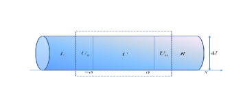
Figure 1: Schematic view of the transversely confined double-barrier model. The dashed-line box C is a hypothetical region including the core device and part of two ideal leads, and L/R symbolize the rest of the leads.

III Numerical Implementation

To illustrate the theoretical formulation proposed above, we consider a quasi-one-dimensional double-barrier model confined transversely to simulate the device system, as shown in Fig. 1. The nonlocal potential is placed only in the region between $-a$ and $a$, and the barriers can be regarded as part of two ideal leads without nonlocal potentials.

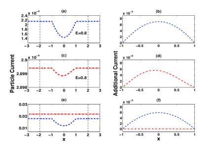
Figure 2: Conventional particle current $I_{c}$ (left column) and additional current $I_{ad}$ (right column) are along the $x$-direction. (a) and (b) are the currents of single-particle with energy $E=0.8$ for the model nonlocal potential $V(x,x^{\prime})$; (c) and (d) are the currents of single-particle with energy $E=0.8$ for our proposed nonlocal potential; (e) and (f) are the total currents of all the particles below the Fermi energy $E_{F}$ calculated with our proposed nonlocal potential (red dash-dot line) and the model nonlocal potential (blue dash line). The vertical dash lines at $x=-2$ and $x=2$ mark the contact regions. Here, $\lambda=0.009$, $\eta=0.01$, and the width of the barriers is $1.0$.

We imagine a central region C (the dashed-line box) that encloses both the core device and the barriers, and the total Hamiltonian for this model can be written as

$$\hat{H}_{tot}=\hat{H}_{0}+\hat{V}_{H}+\hat{V}_{xc},$$ (22)

where $\hat{H}_{0}=\frac{-\hbar^{2}}{2m}\nabla^{2}+U_{0}$ with $U_{0}$ the local potential within the barriers, $\hat{V}_{H}$ is the Hartree potential and $\hat{V}_{xc}$ is the exchange-correlation potential: $\langle\mathbf{r|}\hat{V}_{xc}|\psi\rangle=\int V_{xc}\left(\mathbf{r,r}^{\prime}\right)\psi(\mathbf{r}^{\prime})d\mathbf{r}^{\prime}$. We simplify the potential in Eq. (16) and Eq. (17) to the form of one dimension as

$$V_{H}\left(x\right)=\int{\sum\limits_{k}}v\left(x,x^{\prime}\right)|\psi_{k}\left(x^{\prime}\right)|^{2}dx^{\prime},$$ (23)

and

$$V_{xc}\left(x,x^{\prime}\right)=-{\sum\limits_{k}}v\left(x,x^{\prime}\right)\psi_{k}^{\ast}\left(x\right)\psi_{k}\left(x^{\prime}\right),$$ (24)

where $\psi_{k}\left(x\right)$ is the longitudinal wave function, and

$$v\left(x,x^{\prime}\right) =\int\rho_{1}d\rho_{1}\int\rho_{2}d\rho_{2}\int\frac{d\varphi}{2\pi}$$

$$\text{ \ \ }\times\frac{\varphi^{2}\left(\rho_{1}\right)\varphi^{2}\left(\rho_{2}\right)}{\sqrt{\rho_{1}^{2}+\rho_{2}^{2}-2\rho_{1}\rho_{2}\cos\varphi+\left(x-x^{\prime}\right)^{2}}},$$ (25)

which is averaged over the transverse wave functions.40 A single transverse wave function $\varphi\left(\rho\right)=1/\sqrt{2\pi l^{2}}\exp\left(-\rho^{2}/4l^{2}\right)$ is chosen universally, and a transverse radius $2l$ characterizes the size of the confinement. To proceed, we first solve the energy eigenequation of the double-barrier model with only local potential $U_{0}$ and numerically calculate the wave functions $\psi\left(x\right)$, thus the corresponding Hartree potential $V_{H}$ and exchange-correlation potential $V_{xc}$ of the central region can be constructed from the wave functions by using Eq. (23) and Eq. (24). Then we return to the calculation of the wave functions $\psi\left(x\right)$, and self-consistent calculations are performed using the iterative procedure in the numerical implementation. In general, once all the wave functions with eigenenergies below the Fermi energy $E_{F}$ are known, we can obtain the current density at all points. When the system is under applied bias, the Fermi levels in the left and right leads are taken respectively as $E_{F}+eV$ and $E_{F},$ where $E_{F}$ is the Fermi level in the equilibrium state and $V$ is the bias, i.e., the sums in Eq. (23) and Eq. (24) are up to $E_{F}+eV$ and $E_{F}$ respectively for left-incident and right-incident modes of the functions. Energy unit $\hbar^{2}/2ma^{2}$ is used throughout the calculations as a reduced coefficient, where $a$ is the width of the barrier, $m$ is the mass of the electron. The Fermi energy here is set as $E_{F}=1.0$, and the magnitude of the barriers is fixed to be $U_{0}=6.0$. In addition, all the calculations are preformed in low-temperature limit, i.e., the temperature $T=0$.

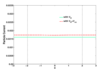
Figure 3: Comparison of the particle currents for each region. The case that involves the proposed nonlocal exchange-correlation potential $V_{xc}$ (dash-dot line) is somewhat a correction to the one that only considers the Hartree potential $V_{H}$ (solid line).

We first study the influences of a model nonlocal potential and our proposed potential in Eq. (17) on the particle currents, respectively. The nonlocal potential is nonzero when $x$ is from $-1$ to $1$, and the barriers are located in $\left[-2,-1\right]$ and $\left[1,2\right]$. The model nonlocal potential here is chosen as $V\left(x,x^{\prime}\right)=\lambda\exp\left[\eta\left(x-x^{\prime}\right)^{2}\right]$, where $\lambda$ and $\eta$ are two independent coefficients. In Fig. 2, we present the calculated currents of left-incoming electrons with a fixed energy $E=0.8$ and below the Fermi energy $E_{F}$, respectively. Here, both the conventional particle current and additional current are given, and the additional currents coming from nonlocal potential $V(x,x^{\prime})$ are calculated by

$$I_{ad}(x)=\frac{-1}{i\hbar}\int_{-1}^{x}dx^{\prime\prime}\int_{-1}^{1}dx^{\prime} \sum\limits_{k}\left[\psi_{k}^{\ast}\left(x^{\prime\prime}\right)V(x^{\prime\prime},x^{\prime})\psi_{k}\left(x^{\prime}\right)\right.$$

$$\text{ \ \ }\left.-\psi_{k}^{\ast}\left(x^{\prime}\right)V(x^{\prime},x^{\prime\prime})\psi_{k}(x^{\prime\prime})\right].$$

From Fig. 2(a) to Fig. 2(d), one can see that for single-particle with the fixed energy the left and right lead currents hold to be constant, while in the central region the currents turn out to be varying with $x$, and the additional currents from the nonlocal potential are nonzero for both the model potential and our proposed potential. It means that in the case of single-particle, the lead currents and the central current calculated with the proposed nonlocal potential behave similarly to that obtained by using the model nonlocal potential, which also violates the conservation. However, Figures 2(e) and 2(f) show that when currents of all incoming electrons below the Fermi energy $E_{F}$ are considered, in the case of the model nonlocal potential the conventional current still violates the continuity condition due to the nonzero additional current, while the conventional currents calculated with the proposed nonlocal potential are seen to be conservative in the whole simulation region and the corresponding additional current vanishes. Moreover, particle currents in all the three regions serve as a minor correction to the ones with Hartree potential only (see Fig. 3).

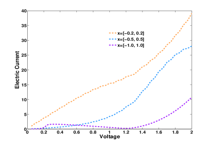
Figure 4: Dependence of the electric currents on the selection of the central region. Nonlocal potential is not included, and the width and magnitude of the barriers are both fixed.

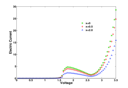
Figure 5: Current properties of different sites of the system with the model nonlocal potential $V_{nl}$. The central region is fixed to be $x=\left[-1,1\right]$, and the barriers are located in $x=\left[-2,-1\right]$ and $x=\left[1,2\right]$. Discrepancies of the currents for all three positions enlarge with the increasing voltage.

Figure 4 plots the dependence of the electric current on the selection of each region. The width of the barriers are fixed as the above while the whole central region is changeable, and the nonlocal potential is absent therein. As we shall see, when the core region is chosen as small as $x=[-0.2,0.2]$, it exhibits a sublinear relation between the current $I$ and the voltage $V$, which is similar to that of a general single-barrier model, and the scattering effect in the central box vanishes. With the increases of the width as $x=\left[-0.5,0.5\right]$ and $x=\left[-1.0,1.0\right]$, the curves shift downwards gradually and finally become nonlinear ones, indicating that careful considerations on relevant area selection must be taken into actual systems to ensure the computational accuracy.

In Fig. 5, we present the $I$-$V$ characteristics of different sites along the $x$ axis when the above model nonlocal potential $V\left(x,x^{\prime}\right)$ is included. Currents of $x=0$, $x=0.5$ and $x=2.0$ differ mutually, as expected, which implies that currents in the central region and the leads calculated with the model nonlocal potential cannot meet the charge conservation. We further explore the contrastive characteristics with our approximation. From Fig. 6, one can see that when only Hartree potential $V_{H}$ is taken into account, currents of the three sites are equal to each other with the increase of the voltage, while the whole of the curve bears an upward shift when the proposed exchange-correlation potential $V_{xc}$ is also considered, and the currents obtained can be still conservative.

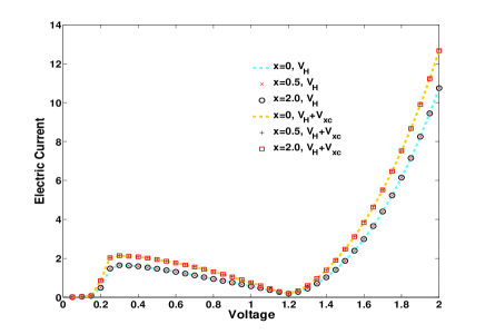
Figure 6: $I$-$V$ characteristics of different sites for: (1) with only Hartree potential $V_{H}$, and (2) with both the Hartree potential $V_{H}$ and the nonlocal exchange-correlation potential $V_{xc}$. The currents obtained from the proposed formalism satisfy the charge conservation.

IV Conclusions and Discussions

In summary, it is of great importance to give correct dynamic charge and potential distributions of the transport systems, which is the key point for the valid currents and prospective applications of molecular devices. Once we are able to calculate the current strictly according to the original Hamiltonian including electron-electron interactions, the problems of charge nonconservation induced by nonlocal potential would not exist, and the results are undoubtedly reasonable. However, it is impossible to obtain rigorous solutions under such intricate interactions. We demonstrate these issues and attest that the nonconservation stems respectively from the improper approximations to electron-electron interactions and the inappropriate definition of current using pseudo wave functions in pseudopotential implementations, and propose a nonlocal-potential formulation of the interactions to fulfill the conservation in the meaning of statistical average, as well as give a verification about the calculation of current in the presence of pseudopotentials. With this method, we have also studied a double-barrier model to simulate the molecular device system, which further confirms our formulation.

Appendix A

Here, we will attempt to give the second quantized form of the nonlocal potential. According to common methods, the wave function $\psi$ can be expanded in terms of a complete basis set $\varphi_{m}$ as

$$\psi\left(\mathbf{r},t\right)=\sum_{m}c_{m}\left(t\right)\varphi_{m}\left(\mathbf{r}\right),$$ (26)

where $c_{m}$ is a coefficient independent of $\mathbf{r}$. Substituting the above wave function into the following Schrödinger equation, which includes the nonlocal potential $V_{xc}(\mathbf{r},\mathbf{r}^{\prime})$,

$$i\hbar\frac{\partial}{\partial t}\psi(\mathbf{r},t)=H_{0}\psi(\mathbf{r},t)+\int d\mathbf{r}^{\prime}V_{xc}(\mathbf{r},\mathbf{r}^{\prime})\psi(\mathbf{r}^{\prime},t),$$ (27)

we have

$$i\hbar\dot{c}_{m}(t)=\sum_{n}H_{0mn}c_{n}(t)+\sum_{n}V_{mn}c_{n}(t),$$ (28)

where

$$H_{0}=\frac{-\hbar^{2}}{2m}\nabla^{2}+v\left(\mathbf{r},t\right),$$ (29)

$$H_{0mn}=\int d\mathbf{r}d\mathbf{r}^{\prime}\varphi_{m}^{\ast}(\mathbf{r})H_{0}\varphi_{n}(\mathbf{r}^{\prime}),$$ (30)

and

$$V_{mn}=\int d\mathbf{r}d\mathbf{r}^{\prime}\varphi_{m}^{\ast}(\mathbf{r})V_{xc}(\mathbf{r},\mathbf{r}^{\prime})\varphi_{n}(\mathbf{r}^{\prime})$$ (31)

is the matrix elements of $V_{xc}(\mathbf{r},\mathbf{r}^{\prime})$. Similarly, the field operator is

$$\hat{\Psi}(\mathbf{r},t)=\sum_{n}\varphi_{n}(\mathbf{r})\hat{a}_{n}(t),$$ (32)

with

$$\hat{a}_{n}(t)=\int d\mathbf{r}\varphi_{n}^{\ast}(\mathbf{r},t)\hat{\Psi}(\mathbf{r},t),$$ (33)

where $\hat{a}_{n}^{{\dagger}}$ $\left(\hat{a}_{n}\right)$ is the creation (annihilation) operator. Therefore, we obtain the second quantized form of the nonlocal potential as

$$\hat{V}_{xc} =\sum_{mn}V_{mn}(t)\hat{a}_{m}^{{\dagger}}(t)\hat{a}_{n}(t)$$

$$=\int d\mathbf{r}d\mathbf{r}^{\prime}\sum_{mn}V_{mn}(t)\varphi_{n}^{\ast}(\mathbf{r},t)\varphi_{m}(\mathbf{r}^{\prime},t)\hat{\Psi}^{{\dagger}}(\mathbf{r}^{\prime},t)\hat{\Psi}(\mathbf{r},t)$$

$$=\int d\mathbf{r}d\mathbf{r}^{\prime}V_{xc}(\mathbf{r}^{\prime},\mathbf{r})\hat{\Psi}^{{\dagger}}(\mathbf{r}^{\prime},t)\hat{\Psi}(\mathbf{r},t).$$ (34)

Appendix B

We first discuss that in introducing the nonlocal pseudopotential, the current calculated with pseudo wave functions does not satisfy the conservation. Pseudopotentials were originally introduced to simplify electronic structure calculations by adding some core functions to the true wave function $\psi\left(\mathbf{r}\right)$ to obtain a smooth pseudo wave function41 ; 42 ; 43

$$\psi\left(\mathbf{r}\right)=\phi\left(\mathbf{r}\right)-\sum\limits_{n}\langle\psi_{n}|\phi\rangle\psi_{n}\left(\mathbf{r}\right),$$ (35)

where $\phi\left(\mathbf{r}\right)$ is the pseudo wave function and $\psi_{n}\left(\mathbf{r}\right)$ is the core function, and the general form of the pseudopotential (only its nonlocal part) is

$$V_{nl}=\sum\limits_{n}(E-E_{n})|\psi_{n}\rangle\langle\psi_{n}|,$$ (36)

from which we obtain

$$\sum\limits_{n}|\psi_{n}\rangle\langle\psi_{n}|=\left(E-H_{0}\right)^{-1}V_{nl}=GV_{nl},$$ (37)

where $G=\left(E-H_{0}\right)^{-1}$ is the Green’s function, and $H_{0}$ is the original Hamiltonian. The true wave function can then be denoted by

$$\psi\left(\mathbf{r}\right) =\langle\mathbf{r}|\psi\rangle$$

$$=\langle\mathbf{r}|\phi\rangle-\langle\mathbf{r}|GV_{nl}|\phi\rangle$$

$$=\phi\left(\mathbf{r}\right)-\int d\mathbf{r}^{\prime\prime}\int d\mathbf{r}^{\prime}\langle\mathbf{r}|G|\mathbf{r}^{\prime}\rangle\langle\mathbf{r}^{\prime}|V_{nl}|\mathbf{r}^{\prime\prime}\rangle\langle\mathbf{r}^{\prime\prime}|\phi\rangle$$

$$=\phi\left(\mathbf{r}\right)-\int d\mathbf{r}^{\prime}d\mathbf{r}^{\prime\prime}G(\mathbf{r,r}^{\prime})V_{nl}(\mathbf{r}^{\prime},\mathbf{r}^{\prime\prime})\phi\left(\mathbf{r}^{\prime\prime}\right).$$ (38)

Therefore, the corresponding Schrödinger equation for the pseudo wave function is

$$H_{0}\phi\left(\mathbf{r}\right)+\int d\mathbf{r}^{\prime}V_{nl}(\mathbf{r,r}^{\prime})\phi\left(\mathbf{r}^{\prime}\right)=E\phi\left(\mathbf{r}\right),$$ (39)

where

$$V_{nl}(\mathbf{r,r}^{\prime}) =\sum\limits_{n}(E-E_{n})\psi_{n}(\mathbf{r})\psi_{n}^{\ast}(\mathbf{r}^{\prime})$$

$$=(E-H_{0})\sum\limits_{n}\psi_{n}(\mathbf{r})\psi_{n}^{\ast}(\mathbf{r}^{\prime}).$$ (40)

It is easy to verify that the conventionally defined current density $\mathbf{J}=\frac{-i\hbar}{2m}[\phi^{\ast}\left(\mathbf{r}\right)\nabla\phi\left(\mathbf{r}\right)-\phi\left(\mathbf{r}\right)\nabla\phi^{\ast}\left(\mathbf{r}\right)]$ along with the obtained pseudo electron density $\rho_{ps}=\left|\phi\left(\mathbf{r}\right)\right|^{2}$ do not meet the charge conservation. Nevertheless, this nonconservation is not caused by introducing the pseudopotential, but is that the above definition of current density cannot be used with the pseudo wave function $\phi\left(\mathbf{r}\right)$. The correct current density must be defined by using the true wave function $\psi\left(\mathbf{r}\right)$. According to the definition $\mathbf{J}_{r}=$ $\frac{-i\hbar}{2m}\left[\psi^{\ast}\left(\mathbf{r}\right)\nabla\psi\left(\mathbf{r}\right)-\psi(\mathbf{r})\nabla\psi^{\ast}(\mathbf{r})\right]$, we get

$$\mathbf{J}_{r}=\mathbf{J}_{ps}+\mathbf{J}_{nl},$$ (41)

where

$$\mathbf{J}_{ps}=\frac{-i\hbar}{2m}\left[\phi^{\ast}\left(\mathbf{r}\right)\nabla\phi\left(\mathbf{r}\right)-\phi\left(\mathbf{r}\right)\nabla\phi^{\ast}\left(\mathbf{r}\right)\right],$$ (42)

and

$$\mathbf{J}_{nl}=\frac{i\hbar}{2m} \left[\phi^{\ast}\left(\mathbf{r}\right)\nabla\Pi(\mathbf{r)+}\Pi(\mathbf{r)}\nabla\phi^{\ast}\left(\mathbf{r}\right)\right.$$

$$\text{ \ \ }\left.-\Pi^{\ast}\left(\mathbf{r}\right)\nabla\Pi(\mathbf{r)-}c.c.\right].$$ (43)

Here, $\Pi(\mathbf{r)=}\int d\mathbf{r}^{\prime}d\mathbf{r}^{\prime\prime}G(\mathbf{r,r}^{\prime})V_{nl}(\mathbf{r}^{\prime},\mathbf{r}^{\prime\prime})\phi\left(\mathbf{r}^{\prime\prime}\right)$. On the basis of Eq. (39), in steady states we can easily give $\nabla\cdot\mathbf{J}_{ps}=-\nabla\cdot\mathbf{J}_{nl}$, which verifies the conservation with the definition of current density in Eq. (41).

References

• (1) J. Paloheimo, P. Kuivalainen, H. Stubb, E. Vuorimaa, and P. Yli-Lahti, Appl. Phys. Lett. 56, 1157(1990).
• (2) L. P. Kouwenhoven, A. T. Johnson, N. C. van der Vaart, C. J. P. M. Harmans, and C. T. Foxon, Phys. Rev. Lett. 67, 1626 (1991).
• (3) J. Chen, M. A. Reed, A. M. Rawlett, and J. M. Tour, Science 286, 1550 (1999).
• (4) C. P. Collier, E. W. Wong, M. BelohradskΓ½, F. M. Raymo, J. F. Stoddart, P. J. Kuekes, R. S. Williams, and J. R. Heath, Science 285, 391 (1999).
• (5) C. Joachim, J. K. Gimzewski, and A. Aviram, Nature 408, 541 (2000).
• (6) J. Park, A. N. Pasupathy, J. I. Goldsmith, C. Chang, Y. Yaish, J. R. Petta, M. Rinkoski, J. P. Sethna, H. D. AbruΓ±a, P. L. McEuen, and D. C. Ralph, Nature 417, 722 (2002).
• (7) N. J. Tao, Nat. Nanotechnol. 1, 173 (2006).
• (8) S. M. Lindsay and M. A. Ratner, Adv. Mater. 19, 23 (2007).
• (9) Y. M. Lin, K. A. Jenkins, A. Valdes-Garcia, J. P. Small, D. B. Farmer, and P. Avouris, Nano Lett. 9, 422 (2009).
• (10) N. Rauhut, M. Engel, M. Steiner, R. Krupke, P. Avouris, and A. Hartschuh, ACS Nano 6, 6416 (2012).
• (11) B. Xu and Y. Dubi, J. Phys.: Condens. Matter 27, 263202 (2015).
• (12) K. Ono, G. Giavaras, T. Tanamoto, T. Ohguro, X. Hu, and F. Nori, Phys. Rev. Lett. 119, 156802 (2017).
• (13) Y. Isshiki, S. Fujii, T. Nishino, and M. Kiguchi, J. Am. Chem. Soc. 140, 3760 (2018).
• (14) R. Landauer, IBM J. Res. Dev. 1, 233 (1957).
• (15) M. BΓΌttiker, Y. Imry, R. Landauer, and S. Pinhas, Phys. Rev. B 31, 6207 (1985).
• (16) A. PrΓͺtre, H. Thomas, and M. BΓΌttiker, Phys. Rev. B 54, 8130 (1996).
• (17) A. P. Jauho, N. S. Wingreen, and Y. Meir, Phys. Rev. B 50, 5528 (1994).
• (18) B. Wang, J. Wang, and H. Guo, Phys. Rev. Lett. 82, 398 (1999).
• (19) J. Taylor, H. Guo, and J. Wang, Phys. Rev. B 63, 245407 (2001).
• (20) M. Brandbyge, J. L. Mozos, P. OrdejΓ³n, J. Taylor, and K. Stokbro, Phys. Rev. B 65, 165401 (2002).
• (21) S. Kurth, G. Stefanucci, C. -O. Almbladh, A. Rubio, and E. K. U. Gross, Phys. Rev. B 72, 035308 (2005).
• (22) C. Y. Yam, X. Zheng, G. H. Chen, Y. Wang, T. Frauenheim, and T. A. Niehaus, Phys. Rev. B 83, 245448 (2011).
• (23) K. Varga, Phys. Rev. B 83, 195130 (2011).
• (24) L. Zhang, B. Wang, and J. Wang, Phys. Rev. B 84, 115412 (2011).
• (25) K. T. Cheung, B. Fu, Z. Z. Yu, and J. Wang, Phys. Rev. B 95, 125422 (2017).
• (26) H. Wang and M. Thoss, J. Chem. Phys. 138, 134704 (2013).
• (27) G. Cabra, A. Jensen, and M. Galperin, J. Chem. Phys. 148, 204103 (2018).
• (28) S. Datta, Quantum Transport: Atom to Transistor, Cambridge University Press, Cambridge (2005).
• (29) V. A. Sablikov and B. S. Shchamkhalova, Phys. Rev. B 58, 13847 (1998).
• (30) V. A. Sablikov, S. V. Polyakov, M. BΓΌttiker, Phys. Rev. B 61, 13763 (2000).
• (31) J. P. Perdew, J. A. Chevary, S. H. Vosko, K. A. Jackson, M. R. Pederson, D. J. Singh, and C. Fiolhais, Phys. Rev. B 46, 6671 (1992).
• (32) C. S. Li, L. H. Wan, Y. D. Wei, and J. Wang, Nanotechnology 19, 155401 (2008).
• (33) L. Zhang, Y. X. Xing, and J. Wang, Phys. Rev. B 86, 155438 (2012).
• (34) D. R. Hamann, M. SchlΓΌter, and C. Chiang, Phys. Rev. Lett. 43, 1494 (1979).
• (35) M. C. Payne, M. P. Teter, D. C. Allan, T. A. Arias, and J. D. Joannopoulos, Rev. Mod. Phys. 64, 1045 (1992).
• (36) R. van Leeuwen, Phys. Rev. Lett. 82, 3863 (1999).
• (37) M. Ruggenthaler and D. Bauer, Phys. Rev. A 80, 052502 (2009).
• (38) Y. Kurzweil and R. Baer, J. Chem. Phys. 121, 8731 (2004).
• (39) S. K. Ghosh and A. K. Dhara, Phys. Rev. A 38, 1149 (1988).
• (40) I. V. Tokatly, Phys. Rev. B 71, 165105 (2005).
• (41) G. Vignale and W. Kohn, Phys. Rev. Lett. 77, 2037 (1996).
• (42) T. B. Boykin, Am. J. Phys. 68, 665 (2000).
• (43) L. Kleinman and D. M. Bylander, Phys. Rev. Lett. 48, 1425 (1982).
• (44) S. W. Gao and Z. Yuan, Phys. Rev. B 72, 121406(R) (2005).
• (45) J. C. Phillips and L. Kleinman, Phys. Rev. 116, 287 (1959).
• (46) Morrel H. Cohen and V. Heine, Phys. Rev. 122, 1821 (1961).
• (47) Neil W. Ashcroft and N. David Mermin, Solid State Physics, Harcourt, Orlando (1976).