Lévy Walks On Finite Intervals: A Step Beyond Asymptotics

Abstract

A Lévy walk of order $\beta$ is studied on an interval of length $L$, driven out of equilibrium by different-density boundary baths. The anomalous current generated under these settings is nonlocally related to the density profile through an integral equation. While the asymptotic solution to this equation is known, its finite-$L$ corrections remain unstudied despite their importance in the study of anomalous transport. Here a perturbative method for computing such corrections is presented and explicitly demonstrated for the leading correction to the asymptotic transport of a Lévy walk of order $\beta=5/3$, which represents a broad universal class of anomalous transport models. Surprisingly, many other physical problems are described by similar integral equations, to which the method introduced here can be directly applied.

I Introduction

The Lévy walk is a popular and well-studied model which describes a variety of physical scenarios in which superdiffusive dynamics lead to nonlocal stationary behavior. Nonlocality is manifested in the mathematical description of the relevant observables in terms of an integral equation with a power-law kernel mandelbrot1982fractal ; drysdale1998levy ; buldyrev2001average ; lepri2011density ; dhar2013exact ; zaburdaev2015levy .

One fruitful application of the Lévy walk model is to the study of anomalous heat transport in one-dimensional (1D) Hamiltonian systems cipriani2005anomalous ; zhao2006identifying ; zoia2007fractional ; lepri2011density ; zaburdaev2011perturbation ; dhar2013exact ; liu2014anomalous ; zaburdaev2015levy . When such systems are constrained to an interval of length $L$ and driven out of equilibrium by heat baths of temperature difference $\Delta T$, one observes an anomalous transport behavior in the asymptotic large-$L$ limit: The energy current $J_{e}$ is found to scale as $J_{e}\sim\Delta T/L^{1-\alpha}$ and the temperature profile is singular at the boundaries. The “anomalous exponent” $\alpha\in\left(0,1\right]$ gets its name from the fact that Fourier’s law predicts $\alpha=0$ grassberger2002heat ; cipriani2005anomalous ; lepri2011density ; dhar2013exact . Active research of anomalous transport focuses on its universal features in the asymptotic limit. The main questions include the classification of models into different universality classes, precisely determining the anomalous exponent $\alpha$ corresponding to each universality class and the relation between $\alpha$ and the singular behavior of the accompanying temperature profiles lepri2011density ; lepri2016heat ; cividini2017temperature .

Although significant progress has recently provided several theoretical predictions for the different universal values of $\alpha$ narayan2002anomalous ; grassberger2002heat ; wang2004intriguing ; cipriani2005anomalous ; lukkarinen2008anomalous ; spohn2014nonlinear ; popkov2015fibonacci , obtaining conclusive experimental support is a difficult problem. Namely, the asymptotic behavior predicted in theory for large-$L$ is hard to reach in numerical simulations and experiments due to finite-size corrections cipriani2005anomalous . In fact, it is generally not known how large a system should be to ensure the asymptotic limit is reached Miron2019 . Indeed, the literature contains numerous observed values of $\alpha$ for a variety of models. These $\alpha$’s are usually extracted from numerical simulations by fitting the observed $L$ dependence of $J_{e}\left(L\right)$ to an inverse power law, assuming that the system is safely inside the asymptotically large-$L$ regime. However, not all simulation results stand in agreement aoki2001fermi ; grassberger2002heat ; li2003anomalous ; wang2004intriguing ; cipriani2005anomalous ; lepri2005studies ; basile2007anomalous , making it difficult to determine the different universality classes and refute incompatible predictions. For this reason, insufficient understanding of finite-size corrections poses a significant hurdle which must be overcome to make progress.

Since Lévy particles are noninteracting, anomalous Lévy walk transport is easier to study than that of Hamiltonian models. Imposing different-density baths similarly gives rise to an anomalous walker current $J$ and a corresponding singular density profile $P\left(x\right)$. This setup was studied in Refs. lepri2011density ; dhar2013exact where an integral equation relating the asymptotic current $J_{0}$ and density profile $P_{0}\left(x\right)$ was formulated and solved exactly in Ref. dhar2013exact . However, finite-size corrections remain unstudied.

In this paper, a perturbative method is presented for computing finite-size corrections to the asymptotic Lévy walk results in three steps: First, the integral equation relating the asymptotic $J_{0}$ and $P_{0}\left(x\right)$ of Ref. dhar2013exact is extended to include finite-size corrections. Then, a perturbative method for computing the corrections order-by-order in inverse powers of $L$ is introduced. Finally, the method is used to explicitly compute the leading correction to the asymptotic $J_{0}$ and $P_{0}\left(x\right)$ for a Lévy walk of order $\beta=5/3$, which is expected to represent a broad universality class of anomalous transport models with exponent $\alpha=1/3$ cipriani2005anomalous . In this case, the asymptotic current $J_{0}$ decays as $J_{0}\sim L^{-2/3}$, whereas its leading correction $J_{1}$ is shown to decay as $J_{1}\sim L^{-1}$. Thus, the asymptotic regime in which $J_{0}\gg J_{1}$ is reached only when $L$ is very large, further illustrating the importance of accounting for finite-size corrections. The intuitive explanation behind the diffusive correction $J_{1}$ is that, although the width of the Lévy walkers’ walk-time distribution diverges, its mean is finite. Thus, although the walkers occasionally undergo very long excursions, most of the walks last a small amount of time, leading to diffusive transport. In an infinite system, the contribution of finite walks vanishes. However, in finite systems they give rise to corrections, the first of which is diffusive transport.

For the reasons noted above, these results constitute a crucial step towards understanding finite-size corrections in anomalous transport and, ultimately, in settling the debate on the different universality classes and the precise values of the corresponding anomalous exponents.

A surprising corollary is that integral equations, which are similar to the one derived for anomalous Lévy walk transport, also show up in many additional physical scenarios. They appear, for example, in the mean first-passage time of Lévy walkers on a finite interval with absorbing boundaries buldyrev2001average , in the anomalous transport of a stochastic 1D gas model Miron2019 , in nonlocal elasticity theory lazopoulos2006non ; carpinteri2011fractional and in the viscosity of polymers in a solvent kirkwood1948intrinsic ; douglas1989surface . As such, the method presented here for studying anomalous Lévy walk transport can be directly applied to a diverse set of problems, spanning across a wide range of research fields.

The paper is organized as follows: The Lévy walk model and nonequilibrium setup are presented in Sec. II. Section III extends the asymptotic results of Ref. dhar2013exact by first deriving a more general integral equation, containing information on both the asymptotic behavior and its corrections, and then presenting a perturbative method for solving it. The method is explicitly used to compute the leading correction to the known asymptotic behavior for the Lévy walk of order $\beta=5/3$ in Sec. IV. Section V provides important details which are relevant when applying the method to other values of $\beta$ and higher order corrections. Concluding remarks follow in Sec. VI.

II The Model

The Lévy walk model of order $\beta$ describes particles moving at a fixed velocity $v$ which evolve via random “walks” of duration $t$ drawn from the distribution

$$\phi\left(t\right)=\beta t_{0}^{\beta}\frac{\theta\left[t-t_{0}\right]}{t^{\beta+1}},$$ (1)

where $1<\beta<2$, $t_{0}$ is the minimal walk-time and $\theta\left[\tau\right]$ is the step function. All but the first moment of $\phi\left(t\right)$ diverge, giving rise to rare, long walks that connect distant points in the system grassberger2002heat ; cipriani2005anomalous ; lepri2011density ; dhar2013exact . The model is studied on a 1D interval parameterized by $x\in\left[0,L\right]$. Following Ref. dhar2013exact , let $P\left(x,t\right)\mathbf{d}x$ denote the number of walkers crossing the interval $\left(x,x+\mathbf{d}x\right)$ at time $t$ and let $Q\left(x,t\right)\mathbf{d}x\mathbf{d}t$ denote the number of walkers whose walk ends inside the interval $\left(x,x+\mathbf{d}x\right)$ during the time interval $\left(t,t+\mathbf{d}t\right)$. Correspondingly, $P\left(x,t\right)$ is called the walker density and $Q\left(x,t\right)$ is called the turning-point density. It will prove useful to consider the rescaled position $x\in\left[0,1\right]$, obtained by dividing the position by $L$.

To model the nonequilibrium settings of anomalous transport, appropriate boundary conditions must be imposed. Following Ref. dhar2013exact , different density walker baths are imposed at the two ends of the system by setting

$$Q\left(x\leq 0\right)=Q_{L}\text{ and }Q\left(x\geq 1\right)=Q_{R}.$$ (2)

With these boundary conditions, the stationary walker current satisfies the integral equation

$$J_{exact}\left(x\right)=\frac{v}{2}\left(Q_{L}\int_{\frac{Lx}{v}}^{\infty}\mathbf{d}\tau\psi\left(\tau\right)-Q_{R}\int_{\frac{L\left(1-x\right)}{v}}^{\infty}\mathbf{d}\tau\psi\left(\tau\right)\right)$$

$$+\frac{L}{2}\int_{0}^{1}\mathbf{d}y\text{ }\mbox{sgn}\left[x-y\right]\psi\left(\frac{L\left|x-y\right|}{v}\right)Q\left(y\right),$$ (3)

where $\psi\left(t\right)$, the probability of drawing a walk-time larger than $t$, is given by

$$\psi\left(t\right)=\int_{t}^{\infty}\mathbf{d}\tau\phi\left(\tau\right)=1+\theta\left[t-t_{0}\right]\left(\left(\frac{t_{0}}{t}\right)^{\beta}-1\right).$$ (4)

Eq. (3) implies that the walker current at position x is the sum of two contributions: The first line describes the contribution coming from the two constant-density walker baths, whereas the second line describes the contributions from walkers inside the system. Since the system is in its steady state, the current must be independent of $x$, i.e. $J_{exact}\left(x\right)\equiv J_{exact}$.

It was also shown in Ref. dhar2013exact that the turning point density $Q\left(x\right)$ satisfies the self-consistent equation

$$Q\left(x\right)=\frac{Q_{L}}{2}\psi\left(\frac{Lx}{v}\right)+\frac{Q_{R}}{2}\psi\left(\frac{L\left(1-x\right)}{v}\right)$$

$$+\frac{L}{2v}\int_{0}^{1}\mathbf{d}y\phi\left(\frac{L\left|x-y\right|}{v}\right)Q\left(y\right),$$ (5)

and that the turning point density $Q\left(x\right)$ is related to the walker density $P\left(x\right)$ by

$$P\left(x\right)=\frac{\beta t_{0}}{\beta-1}Q\left(x\right)+\mathcal{O}\left(\varepsilon^{\beta-1}\right),$$ (6)

where $\varepsilon=t_{0}v/L$ plays the role of a dimensionless inverse system-size. Eqs. (3), (5) and (6) constitute the starting point of this study.

III A Step Beyond Asymptotics

Since the solution of Eq. (3) for $J_{exact}$ is hard to compute, the first step is to expand the equation in small $\varepsilon$

$$J\approx A\varepsilon P^{\prime}\left(x\right)-B\varepsilon^{\beta-1}\int_{0}^{1}\mathbf{d}y\frac{P^{\prime}\left(y\right)}{\left|x-y\right|^{\beta-1}},$$ (7)

where $A=\frac{v\left(\beta-1\right)}{2\left(2-\beta\right)}$, $B=\frac{v}{2\beta}$, $P^{\prime}\left(x\right)$ denotes the derivative of $P\left(x\right)$. Note that corrections of $\mathcal{O}\left(\varepsilon^{2\left(\beta-1\right)}\right)$ have been neglected and will be addressed later in Sec. V (also see Appendix A). Equation (7) is derived by substituting $\psi\left(t\right)$ into Eq. (3) for $J_{exact}$, expanding up to linear order in $\varepsilon$ and employing the relation between $P\left(x\right)$ and $Q\left(x\right)$ of Eq. (6). A similar equation for A = 0 was derived in Ref. dhar2013exact .

Before proceeding to solve Eq. (7), let us first establish some useful notations. The rightmost term in Eq. (7) is intuitively called the “nonlocal” term since it depends on the values of $P^{\prime}\left(x\right)$ across the entire system. Naturally, the term $A\varepsilon P^{\prime}\left(x\right)$ is then referred to as the “local” term and $J$ is called the “source” term. The integral Eq. (7) for $J$ is a weakly singular Fredholm integral equation (WSFIE) of the second kind kress1989linear ; moiseiwitsch2011integral ; zemyan2012classical . It is called weakly singular since the integral kernel diverges for $y=x$ yet, since $0<\beta-1<1$, the singularity is integrable. Last, when the unknown function appears both under the integral sign and outside the integral, the equation is of the “second kind” but if it appears only under the integral sign, it is of the “first kind”. Note that an equation for $J$, containing both a local term $\sim\mathcal{O}\left(\varepsilon^{-1}\right)$ and a non-local term $\sim\mathcal{O}\left(\varepsilon^{\beta-1}\right)$, is obtained whenever the walk-time distribution $\phi\left(t\right)$ contains a short walk-time cutoff mechanism.

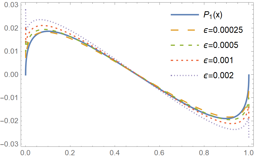
Figure 1: A comparison between the density profile $P_{1}\left(x\right)$ of Eq. (13) and the collapse of $\varepsilon^{1/3}\left(P_{Num}\left(x\right)-P_{0}\left(x\right)\right)$ for different values of the inverse system size $\varepsilon$. The two are expected to identify as $\varepsilon\rightarrow 0$.

The simplest way to proceed is to take the asymptotic $\varepsilon\rightarrow 0$ limit in Eq. (7). In this limit the local term vanishes from Eq. (7), and with it all information about finite-size corrections, reducing the equation to the WSFIE of the first kind studied in Ref. dhar2013exact . Although this WSFIE can indeed be solved exactly by the Sonin formula samko1993fractional ; buldyrev2001average , the trade-off is that finite-size corrections remain out of reach.

Here, a method which preserves information about finite size corrections is suggested instead. This method relies on the interplay between the local term $\propto\varepsilon$ and the nonlocal term $\propto\varepsilon^{\beta-1}$ to construct an ansatz for $P^{\prime}\left(x\right)$ and $J$ in the form of a power-series in $\varepsilon^{\beta-2}$, the ratio of the two scales, as

$$\begin{cases}P^{\prime}=P_{0}^{\prime}+\varepsilon^{2-\beta}P_{1}^{\prime}+\varepsilon^{2\left(2-\beta\right)}P_{2}^{\prime}+...\\ J=\varepsilon^{\beta-1}\left[\mathcal{J}_{0}+\varepsilon^{2-\beta}\mathcal{J}_{1}+\varepsilon^{2\left(2-\beta\right)}\mathcal{J}_{2}+...\right]\end{cases},$$ (8)

where $P_{n}^{\prime}\left(x\right)$ and $\mathcal{J}_{n}$ are independent of $\varepsilon$. In turn, this allows replacing Eq. (7) by a hierarchy of WSFIEs of the first kind

$$\begin{cases}\mathcal{J}_{0}=-B\int_{0}^{1}\mathbf{d}y\frac{P_{0}^{\prime}\left(y\right)}{\left|x-y\right|^{\beta-1}}&\text{at }\text{$\mathcal{O}\left(\varepsilon^{\beta-1}\right)$}\\ \mathcal{J}_{1}=AP_{0}^{\prime}\left(x\right)-B\int_{0}^{1}\mathbf{d}y\frac{P_{1}^{\prime}\left(y\right)}{\left|x-y\right|^{\beta-1}}&\text{at }\text{$\mathcal{O}\left(\varepsilon\right)$}\\ \vdots\\ \mathcal{J}_{n}=AP_{n-1}^{\prime}\left(x\right)-B\int_{0}^{1}\mathbf{d}y\frac{P_{n}^{\prime}\left(y\right)}{\left|x-y\right|^{\beta-1}}&\text{at }\mathcal{O}\left(\varepsilon^{\left(\beta-1\right)+\left(2-\beta\right)n}\right)\end{cases}$$ (9)

where many of which can be solved using the Sonin formula samko1993fractional ; buldyrev2001average . The first hierarchy equation, at $\mathcal{O}\left(\varepsilon^{\beta-1}\right)$, coincides with the asymptotic equation of Ref. dhar2013exact while the rest provide increasingly higher-order, finite-size corrections which must be solved in an iterative fashion. It is important to stress that this method can be extended to additional WSFIEs of the second kind which exhibit a similar interplay between the local and nonlocal terms, even when the constant source term, e.g., $J$ in Eq. (7), is replaced by a sufficiently well-behaved function of $x$ (see Appendix B). In particular, it can be directly applied to the problems mention in Sec. I kirkwood1948intrinsic ; douglas1989surface ; lazopoulos2006non ; carpinteri2011fractional ; Miron2019 .

IV The Leading Correction For $\beta=5/3$

This method is next used to compute the leading correction to the asymptotic density profile and current for a Lévy walk of order $\beta=\frac{5}{3}$. The generalization to different values of β and higher-order corrections is then discussed in Sec. V.

Applying the ansatz

$$\begin{cases}P^{\prime}\left(x\right)=P_{0}^{\prime}\left(x\right)+\varepsilon^{1/3}P_{1}^{\prime}\left(x\right)+\mathcal{O}\left(\varepsilon^{2/3}\right)\\ J=\varepsilon^{2/3}\mathcal{J}_{0}+\varepsilon\mathcal{J}_{1}+\mathcal{O}\left(\varepsilon^{4/3}\right)\end{cases},$$ (10)

to Eq. (7) for $J$ yields a hierarchy of WSFIEs of the first kind. The first equation, appearing at $\mathcal{O}\left(\varepsilon^{2/3}\right)$, is simply the asymptotic equation studied in Ref. dhar2013exact . The solution is obtained by applying the Sonin formula samko1993fractional ; buldyrev2001average (see Appendix B) and enforcing the boundary conditions in Eq. (2). One finds

$$P_{0}^{\prime}\left(x\right)=-\frac{b\mathcal{J}_{0}}{v\left(x\left(1-x\right)\right)^{1/6}}\text{ }\text{and}\text{ }\mathcal{J}_{0}=-\frac{av\Delta P}{b}$$ (11)

where $a=\Gamma\left[\frac{5}{3}\right]/\Gamma\left[\frac{5}{6}\right]^{2}$, $b=\frac{5}{3\pi}$, $\Gamma\left[x\right]$ is the gamma function and $\Delta P\equiv P_{R}-P_{L}=\frac{5t_{0}}{2}\left(Q_{R}-Q_{L}\right)$ follows from Eq. (6).

To step beyond the known asymptotic results, let us consider the next hierarchy equation for the leading correction, $P_{1}^{\prime}\left(x\right)$. This equation appears at $\mathcal{O}\left(\varepsilon\right)$ and is given by

$$\frac{10}{3v}\left(vP_{0}^{\prime}\left(x\right)-\mathcal{J}_{1}\right)=\int_{0}^{1}\mathbf{d}y\frac{P_{1}^{\prime}\left(y\right)}{\left|x-y\right|^{2/3}}.$$ (12)

Due to the hierarchical structure of the ansatz of Eq. (10), $P_{0}^{\prime}\left(x\right)$ enters this equation as a source term. Equation (12) is also a WSFIE of the first kind since $P_{1}^{\prime}\left(x\right)$ appears only inside the integral. Applying the Sonin formula samko1993fractional ; buldyrev2001average yields

$$P_{1}^{\prime}\left(x\right)=-\frac{b}{v}\left(\frac{\mathcal{J}_{1}}{\left(x\left(1-x\right)\right)^{1/6}}+\frac{av\Delta P}{3^{1/2}2^{1/3}}I\left(x\right)\right),$$ (13)

where $\varepsilon\mathcal{J}_{1}$ is the yet-unknown leading corrections to the asymptotic current and $I\left(x\right)$ is given by

$$I\left(x\right)=\frac{1}{x^{\frac{1}{6}}}\frac{d}{dx}\int_{x}^{1}\frac{\mathbf{d}tt^{\frac{1}{3}}}{\left(t-x\right)^{\frac{1}{6}}}\frac{d}{dt}\int_{0}^{t}\frac{\mathbf{d}q\left(1-q\right)^{-\frac{1}{6}}}{q^{\frac{1}{3}}\left(t-q\right)^{\frac{1}{6}}}.$$ (14)

Manipulating $I\left(x\right)$ to its closed form requires careful treatment since Eq. (14) contains nontrivial improper integrals. One finds

$$I\left(x\right)=-\frac{2^{2/3}}{\left(x\left(1-x\right)\right)^{1/6}}-\frac{16x^{5/6}}{2^{1/3}5\left(1-x\right)^{7/6}}\biggl{(}G_{+}\left(x\right)$$

$$-\frac{5\left(2x+1\right)}{16x}G_{-}\left(x\right)\biggl{)}-\frac{\left(2x+1\right)\left(H_{+}\left(x\right)+H_{-}\left(x\right)\right)}{2\sqrt{x}\left(1-x\right)^{7/6}}$$

$$+\frac{16\Gamma\left[\frac{5}{6}\right]\Gamma\left[\frac{8}{3}\right]\left(K_{+}\left(x\right)-K_{-}\left(x\right)\right)}{15\sqrt{\pi}\left(1-x\right)^{7/6}}$$ (15)

where $G_{\pm}\left(x\right)=F_{1}\left[\frac{7}{6}\pm\frac{1}{2};\frac{1}{6},\frac{1}{6};\frac{13}{6}\pm\frac{1}{2};\frac{2\sqrt{x}}{\sqrt{x}-1},\frac{2\sqrt{x}}{\sqrt{x}+1}\right]$, $H_{\pm}\left(x\right)=\left(1\pm\sqrt{x}\right)^{2/3}F_{1}\left[\frac{2}{3};\frac{1}{6},\frac{1}{6};\frac{5}{3};\frac{\sqrt{x}\pm 1}{\sqrt{x}\mp 1},1\right]$ and $K_{\pm}\left(x\right)=\left(1\pm\sqrt{x}\right)^{5/3}\mbox{ }_{2}F_{1}\left[\frac{1}{6},\frac{5}{3};\frac{5}{2};\frac{\sqrt{x}\pm 1}{\sqrt{x}\mp 1}\right]$. Here $F_{1}\left[a;b_{1},b_{2};c;z_{1},z_{2}\right]$ is the Appell hypergeometric function and $\mbox{ }_{2}F_{1}\left[a;b;c;z\right]$ is the hypergeometric function of the second kind.

The function $I\left(x\right)$ has two interesting properties: First, it is easy to show that the hierarchy equation (12) is symmetric under reflections $x\rightarrow 1-x$ and so $I\left(x\right)$ must too respect this symmetry. Induction can be used to extend this argument to all hierarchy equations (see Appendix B). Second, one can also show that, near the left boundary of the system, $I\left(x\right)$ behaves as

$$I\left(x\rightarrow 0\right)\propto x^{-1/2}+\mathcal{O}\left(x^{-1/6}\right).$$ (16)

This implies that, for any finite $\varepsilon$, the boundary singularity of the leading correction $P_{1}^{\prime}\left(x\right)$ dominates over that of the asymptotic solution $P_{0}^{\prime}\left(x\right)$.

Having found the closed-form solution for $P_{1}^{\prime}\left(x\right)$, the final step is to determine $\mathcal{J}_{1}$. This is done by integrating Eq. (13) for $P_{1}\left(x\right)$ with the appropriate boundary conditions. Since the asymptotic results already use $P_{0}\left(1\right)-P_{0}\left(0\right)=\Delta P$ in Eq. (11), the corrections must satisfy $P_{n}\left(0\right)=P_{n}\left(1\right)=0$ for all $n>0$. With these boundary conditions, $\mathcal{J}_{1}$ is given by

$$\mathcal{J}_{1}=2^{4/3}3^{-1/2}av\Delta P.$$ (17)

Substituting $\mathcal{J}_{1}$ back inside Eq. (13) for $P_{1}^{\prime}\left(x\right)$ yields the final expression for the leading density gradient correction:

$$P_{1}^{\prime}\left(x\right)=-\frac{ab\Delta P}{3^{1/2}2^{1/3}}\left(\frac{2^{5/3}}{\left(x\left(1-x\right)\right)^{1/6}}+I\left(x\right)\right).$$ (18)

Collecting these results into the ansatz in Eq. (10) gives the two leading contributions to the anomalous current and density profile of the Lévy walk of order $5/3$”

$$\begin{cases}P^{\prime}\left(x\right)\approx a\Delta P\biggl{[}\left(x\left(1-x\right)\right)^{-1/6}-\frac{b}{2^{1/3}3^{1/2}}\\ \text{ }\times\varepsilon^{1/3}\left(2^{5/3}\left(x\left(1-x\right)\right)^{-1/6}+I\left(x\right)\right)\biggl{]}\\ J\approx-\frac{a}{b}v\Delta P\varepsilon^{2/3}\left(1-\frac{2^{4/3}b}{3^{1/2}}\varepsilon^{1/3}\right)\end{cases}.$$ (19)

Equations (17) and (18) are the first finite-size corrections computed in the context of anomalous transport. To verify that $P_{1}^{\prime}\left(x\right)$ and $\mathcal{J}_{1}$ indeed describe the leading correction to the asymptotic results in Eq. (11), they are compared to the numerical solutions of the exact Lévy walk model equations. These are Eq. (3) for $J_{exact}$, Eq. (5) for $Q\left(x\right)$ and Eq. (6) which relates $Q\left(x\right)$ to $P\left(x\right)$ as $P\left(x\right)=\frac{\beta t_{0}}{\beta-1}Q\left(x\right)+\mathcal{O}\left(\varepsilon^{\beta-1}\right)$. In Ref . dhar2013exact the exact self-consistent equations for $P\left(x\right)$ and $Q\left(x\right)$ were numerically solved and shown to agree with Eq. (6). Figure 1 shows $P_{1}\left(x\right)$ alongside the collapse of $\varepsilon^{1/3}\left(P_{Num}\left(x\right)-P_{0}\left(x\right)\right)$ for different values of $\varepsilon$. $P_{Num}\left(x\right)$ is obtained by numerically solving Eq. (5) for $Q_{Num}\left(x\right)$ and then using Eq. (6) to relate $Q_{Num}\left(x\right)$ to $P_{Num}\left(x\right)$. Notice that the matching to $P_{1}\left(x\right)$ breaks down near the endpoints. Indeed, the derivation of the approximate relation between $J$ and $P\left(x\right)$ in Eq. (7) is valid only for $x\in\left[\varepsilon,1-\varepsilon\right]$ and, consequently, so is its solution (see Appendix B). Specifically, the behavior of $P\left(x\right)$ in the intervals $x\in\left[0,\varepsilon\right)\cup\left(1-\varepsilon,1\right]$ unfortunately remains out of reach. The same difficulties were reported in Ref. buldyrev2001average , which studies the closely related problem of computing the mean first-passage time for the Lévy walk. Nevertheless, it is straightforward to show that limiting the domain of $x$ to $\left[\varepsilon,1-\varepsilon\right]$ does not introduce new corrections. Figure 2 compares $J$ of Eq. (19) to the asymptotic current $J_{0}=\varepsilon^{2/3}\mathcal{J}_{0}$ and to the exact current $J_{exact}$, obtained by numerically solving Eq. (5) for $Q\left(x\right)$ and substituting the result into Eq. (3) for $J_{exact}$.

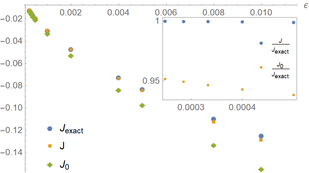
Figure 2: The current $J$ predicted in Eq. (19) (blue circles) is compared to the asymptotic current $J_{0}$ of Eq. (11) (orange squares) and to the exact current $J_{exact}$ (green diamonds) which is obtained by numerically solving $Q\left(x\right)$ of Eq. (5) and substituting the solution into Eq. (3). Inset: The ratios $\frac{J}{J_{exact}}$ (blue circles) and $\frac{J_{0}}{J_{exact}}$ (orange squares) are compared. The parameters are $v=t_{0}=1$ and $\Delta Q=1\rightarrow\Delta P=5/2$.

V Other $\beta$ Values and Higher Order Corrections

Let us finally discuss the application of this method to other values of$\beta$ and higher-order corrections. For a general $\beta$ and arbitrary order, this method faces two caveats: The first is due to the fact that Eq. (7) for $J$ is a small-$\varepsilon$ approximation of Eq. (3) for $J_{exact}$, implying that some higher-order corrections must have been neglected in its derivation. The second follows from limitations on the source term’s behavior at the boundaries that are imposed by the Sonin formula. These two caveats are explained next and additional details are provided in Appendix B.

The appropriate ansatz for $P^{\prime}\left(x\right)$ and $J$ for a Lévy walk of order $\beta$ is

$$\begin{cases}P^{\prime}\left(x\right)=\sum_{m=0}^{M}\varepsilon^{\left(2-\beta\right)m}P_{m}^{\prime}\left(x\right)+\mathcal{O}\left(\varepsilon^{\left(2-\beta\right)\left(M+1\right)}\right)\\ J=\varepsilon^{\beta-1}\left[\sum_{m=0}^{M}\varepsilon^{\left(2-\beta\right)m}\mathcal{J}_{m}+\mathcal{O}\left(\varepsilon^{\left(2-\beta\right)\left(M+1\right)}\right)\right]\end{cases},$$ (20)

where $M$ is the maximal expansion order beyond which the method is no longer accurate. $M$ is the manifestation of the first caveat mentioned above. From Eqs. (20) and (9), one learns that the hierarchy equation for $P_{M}^{\prime}\left(x\right)$ is of $\mathcal{O}\left(\varepsilon^{\beta-1+\left(2-\beta\right)M}\right)$. Thus, to determine $M$ we must account for the terms neglected in the derivation of Eq. (7) for $J$ (see Appendix A) and find the order at which they enter the equation for $P_{M}^{\prime}\left(x\right)$. Appendix A shows that the leading $\mathcal{O}\left(\varepsilon^{2\left(\beta-1\right)}\right)$ corrections in Eq. (7) set $M=\left\lceil\frac{\beta-1}{2-\beta}\right\rceil$.

It is important to stress that the hierarchy equations for $P^{\prime}_{m}\left(x\right)$ are perfectly accurate for $0\leq m<M$. Moreover, if only the anomalous current $J$ is of interest, one can significantly increase $M$ by working directly with Eq. (24). Then the $\mathcal{O}\left(\varepsilon^{2\left(\beta-1\right)}\right)$ corrections are replaced by $\mathcal{O}\left(\varepsilon^{3}\right)$ corrections and $M$ increases to $M=\left\lceil\frac{4-\beta}{2-\beta}\right\rceil$.

The second caveat is intrinsic to the Sonin formula. As explained in Ref, samko1993fractional , the Sonin formula applies only when the source term’s boundary singularity is weaker than the kernel’s singularity. Depending on the value of $\beta$, some of the hierarchy equations might not satisfy this requirement, even for $m<M$. Equation (9) shows that the source term in the hierarchy equation for $P_{m}^{\prime}\left(x\right)$ is proportional to $P_{m-1}^{\prime}\left(x\right)$. In Appendix B, the boundary behavior of $P_{m-1}^{\prime}\left(x\right)$ is argued to be of the form $P_{m-1}^{\prime}\left(x\rightarrow 0\right)\propto x^{\left(2m-1\right)\left(\frac{\beta-2}{2}\right)}$ for general $m$ and $\beta$, with similar behavior for $x\rightarrow 1$. Comparing this singularity to the kernel’s singularity $\beta-1$ restricts the Sonin formula to $m<\frac{\beta}{2\left(2-\beta\right)}$.

Nevertheless, since all hierarchy equations satisfying $0\leq m<M$ are precise, hierarchy equations for $P_{m}^{\prime}\left(x\right)$ with $\frac{\beta}{2\left(2-\beta\right)}<m<M$ can still be solved by any other method, be it analytical or numerical, and yield the correction solutions.

VI Conclusions

In this paper, the anomalous transport properties of a 1D Lévy walk of order $\beta$ are studied on a finite interval of size $L$ under nonequilibrium settings. Extending the work of Ref. dhar2013exact , which related the anomalous walker current $J$ to the density gradient $P^{\prime}\left(x\right)$ for asymptotically large $L$, a more general integral equation which also captures finite-size corrections is derived. A perturbative method is presented for constructing an order-by-order solution of this equation. The method is explicitly demonstrated by computing the leading correction to the asymptotic behavior for $\beta=5/3$, and its results are shown to be in excellent agreement with the numerical solution of the exact equations.

Remarkably, many other physical problems are described by similar integral equations kirkwood1948intrinsic ; douglas1989surface ; lazopoulos2006non ; carpinteri2011fractional ; Miron2019 , bringing hope that the method presented here could be used in a verity of different fields. In the context of anomalous transport, it is interesting to compare the results computed here to simulations and experiments. This could test if Lévy walks are indeed a reliable model for anomalous transport, even beyond the asymptotic limit. Applying this method to study additional Lévy walk properties, as well as other physical problems, is an equally interesting and exciting prospect.

VII Acknowledgments

I would like to thank my advisor D. Mukamel for his ongoing encouragement, help, and support. I also thank O. Raz and V. V. Prasad for critical reading of this manuscript as well as G. Falkovich for helpful comments. In addition, previous projects with Anupam Kundu and Julien Cividini have significantly influenced this study, and their collaboration is greatly appreciated. This work was supported by a research grant from the Center of Scientific Excellence at the Weizmann Institute of Science.

Appendix A - The Derivation of Eq. (7)

Equation (3) for $J_{exact}$ was derived in Ref. dhar2013exact and serves as the basis for the derivation of Eq. (7) for $J$ and mainly differs in the treatment of the finite-size corrections. The key steps of the derivation are outlined next.

Using $\psi\left(t\right)$ of Eq. (4), the second line of Eq. (3) for $J_{exact}$ becomes

$$\frac{L}{2}\int_{0}^{1}\mathbf{d}y\text{ }\mbox{sgn}\left[x-y\right]\psi\left(\frac{L\left|x-y\right|}{v}\right)Q\left(y\right)$$

$$=\frac{L}{2}\left(\int_{x-\varepsilon}^{x}\mathbf{d}y\text{ }Q\left(y\right)-\int_{x}^{x+\varepsilon}\mathbf{d}y\text{ }Q\left(y\right)\right)$$

$$+\frac{L\varepsilon^{\beta}}{2}\left(\int_{0}^{x-\varepsilon}\frac{\mathbf{d}yQ\left(y\right)}{\left(x-y\right)^{\beta}}-\int_{x+\varepsilon}^{1}\frac{\mathbf{d}yQ\left(y\right)}{\left(y-x\right)^{\beta}}\right).$$ (21)

Expanding the second line of Eq. (21) in small $\varepsilon$ yields

$$-\frac{t_{0}v\varepsilon}{2}Q^{\prime}\left(x\right)+\mathcal{O}\left(\varepsilon^{3}\right)$$ (22)

and integrating the third line by parts yields

$$\frac{t_{0}v\varepsilon}{2-\beta}Q^{\prime}\left(x\right)+\frac{t_{0}v\varepsilon^{\beta-1}}{2\left(\beta-1\right)}$$

$$\times\left(\frac{Q\left(1\right)}{\left(1-x\right)^{\beta-1}}-\frac{Q\left(0\right)}{x^{\beta-1}}-\int_{0}^{1}\frac{\mathbf{d}yQ^{\prime}\left(y\right)}{\left|x-y\right|^{\beta-1}}\right)+\mathcal{O}\left(\varepsilon^{3}\right),$$ (23)

where $Q\left(0\right)=Q_{L}$ and $Q\left(1\right)=Q_{R}$ follow from Eq. (2). Collecting these terms back into $J_{exact}$ gives

$$J=\frac{t_{0}v\beta\varepsilon Q^{\prime}\left(x\right)}{2\left(2-\beta\right)}-\frac{t_{0}v\varepsilon^{\beta-1}}{2\left(\beta-1\right)}\int_{0}^{1}\frac{\mathbf{d}yQ^{\prime}\left(y\right)}{\left|x-y\right|^{\beta-1}}+\mathcal{O}\left(\varepsilon^{3}\right).$$ (24)

To obtain Eq. (7), which relates $J$ and $P^{\prime}\left(x\right)$, one uses the relation $P\left(x\right)=\frac{\beta t_{0}}{\beta-1}Q\left(x\right)+\mathcal{O}\left(\varepsilon^{\beta-1}\right)$ in Eq. (6), which inevitably introduces corrections of $\mathcal{O}\left(\varepsilon^{2\left(\beta-1\right)}\right)$ into Eq. (24).

Two important comments are in order: The first is that Eq. (7) is valid only for $\beta>\frac{3}{2}$ due to the neglected $\mathcal{O}\left(\varepsilon^{2\left(\beta-1\right)}\right)$ corrections. The second is that the manipulations involved in going from Eq. (21) to Eq. (7) are valid only for $x\in\left[\varepsilon,1-\varepsilon\right]$. This implies that the density profiles in Eq. (19) are not accurate for $x\in\left[0,\varepsilon\right)\cup\left(1-\varepsilon,1\right]$.

Appendix B - The Sonin Formula and Its Solubility Condition

VII.0.1 The Sonin Formula

The Sonin formula provides the formal solution to a class of WSFIEs of the first kind. Specifically, it can be used to solve equations of the form

$$h\left(x\right)=\int_{0}^{1}\mathbf{d}y\frac{\varphi\left(y\right)}{\left|x-y\right|^{\beta-1}}$$ (25)

for $\varphi\left(x\right)$ where $1<\beta<2$. For the purpose of this study, it is sufficient to only consider source terms $h\left(x\right)$ which are symmetric under reflections $x\rightarrow 1-x$ and are of the form

$$h\left(x\right)=\frac{h^{*}\left(x\right)}{\left(x\left(1-x\right)\right)^{\left(\beta-1\right)-\gamma}},$$ (26)

where $h^{*}\left(x\right)$ a smooth function of $x$ and $0<\gamma<\beta-1$. The latter condition means that the Sonin formula applies only when the source term’s boundary singularity is weaker than the kernel’s singularity. For $\gamma$ and $h\left(x\right)$ satisfying these conditions, the Sonin formula yields the solution

$$\varphi\left(x\right)=\frac{\mathcal{B}}{x^{\frac{2-\beta}{2}}}\frac{d}{dx}\int_{x}^{1}\frac{\mathbf{d}tt^{2-\beta}}{\left(t-x\right)^{\frac{2-\beta}{2}}}\frac{d}{dt}\int_{0}^{t}\frac{\mathbf{d}qq^{\frac{\beta-2}{2}}h\left(q\right)}{\left(t-q\right)^{\frac{2-\beta}{2}}}$$ (27)

where $\mathcal{B}=-\frac{\sin\left[\frac{\pi\beta}{2}\right]\Gamma\left[\beta-1\right]}{\pi\Gamma\left[\frac{\beta}{2}\right]^{2}}$ and $\Gamma\left[x\right]$ is the gamma function. It is important to stress that the Sonin formula applies to far more general WSFIE’s of the first kind. An extensive account and further details can be found in Refs. samko1993fractional ; buldyrev2001average ; dhar2013exact .

VII.0.2 Solubility Condition

Next, the implications of the requirements on the boundary singularity of $h\left(x\right)$ of Eq. (26) are discussed. Consider the hierarchy of integral equations obtained by substituting the ansatz of Eq. (20) into Eq. (7). The first equation is

$$-\frac{2\beta\mathcal{J}_{0}}{v}=\int_{0}^{1}\mathbf{d}y\frac{P_{0}^{\prime}\left(y\right)}{\left|x-y\right|^{\beta-1}}$$ (28)

and its constant source term trivially satisfies the requirements in Eq. (26). Imposing the boundary conditions in Eq. (2) provides the asymptotic solution

$$P_{0}^{\prime}\left(x\right)=\frac{\Gamma\left[\beta\right]\Delta P}{\Gamma\left[\frac{\beta}{2}\right]^{2}\left(x\left(1-x\right)\right)^{\frac{2-\beta}{2}}}.$$ (29)

The next equation, now for the leading correction $P_{1}^{\prime}\left(x\right)$, is

$$\beta\left(\frac{\beta-1}{2-\beta}P_{0}^{\prime}\left(x\right)-\frac{2}{v}\mathcal{J}_{1}\right)=\int_{0}^{1}\mathbf{d}y\frac{P_{1}^{\prime}\left(y\right)}{\left|x-y\right|^{\beta-1}}.$$ (30)

The only nonconstant source term in this equation is $\propto P_{0}^{\prime}\left(x\right)$. The range of $\beta$ for which its singularity is weaker than that of the kernel is

$$\beta>\frac{4}{3}.$$ (31)

As such, the leading correction $P_{1}^{\prime}\left(x\right)$ can be computed from the Sonin formula for any $\beta$ in this range.

The general equation for $P_{m}^{\prime}\left(x\right)$,

$$c_{1}P_{m-1}^{\prime}\left(x\right)-c_{2}\mathcal{J}_{m}=\int_{0}^{1}\mathbf{d}y\frac{P_{m}^{\prime}\left(y\right)}{\left|x-y\right|^{\beta-1}},$$ (32)

with $c_{1}=\frac{2\beta}{v}\frac{v\left(\beta-1\right)}{2\left(2-\beta\right)}$ and $c_{2}=\frac{2\beta}{v}$, is used next to find the range of allowed $\beta$ at any order $m$. To this end, let us take the leading singular behavior of the source term $P_{m-1}^{\prime}\left(x\right)$ to be $\propto\left(x\left(1-x\right)\right)^{-\gamma}$. For $P_{m-1}^{\prime}\left(x\right)$ to satisfy the requirements of Eq. (26), $\gamma$ can only take values in $0<\gamma<\beta-1$. The solution of this equation via the Sonin formula is

$$P_{m}^{\prime}\left(x\right)\propto-x^{\frac{\beta-2}{2}}\frac{d}{dx}\int_{x}^{1}\mathbf{d}t\frac{t^{2-\beta}Y\left(t\right)}{\left(t-x\right)^{\frac{2-\beta}{2}}}$$ (33)

where

$$Y\left(t\right)=\frac{d}{dt}\int_{0}^{t}\mathbf{d}q\frac{\left(q\left(1-q\right)\right)^{-\gamma}}{\left(q\left(t-q\right)\right)^{\frac{2-\beta}{2}}}$$ (34)

and the term $\propto\mathcal{J}_{m-1}$ was neglected since its boundary singularity is trivially weaker than that of $\left(x\left(1-x\right)\right)^{-\gamma}$.

To continue, note that, although not manifest in Eq. (7), the hierarchy ansatz reveals the symmetry of $P^{\prime}\left(x\right)$ under reflections $x\rightarrow 1-x$. To see this, note that the source term in Eq. (28) for $P_{0}^{\prime}\left(x\right)$ is independent of $x$. It is easy to show that this equation is symmetric under $x\rightarrow 1-x$ and so is its solution. Next, since $P_{0}^{\prime}\left(x\right)$ is the only nonconstant source term in Eq. (30) for $P_{1}^{\prime}\left(x\right)$, one can show that $P_{1}^{\prime}\left(x\right)$ must too be symmetric under inversion. Using induction one can show this symmetry propagates throughout the entire hierarchy. It is thus sufficient to consider the behavior of $P_{m}^{\prime}\left(x\right)$ for $x\rightarrow 0$. One can then use Eq. (33) to show that the leading boundary singularity of $P_{m}^{\prime}\left(x\right)$ is

$$P_{m}^{\prime}\left(x\rightarrow 0\right)\propto x^{\beta-2-\gamma}.$$ (35)

By comparing Eq. (35) to the boundary singularity for the first few values of $m$, the range of allowed $\beta$ for any order $m$ can be obtained: The boundary singularity of $P_{1}^{\prime}\left(x\right)$, whose source term is $\propto\left(x\left(1-x\right)\right)^{\frac{\beta-2}{2}}$, is found by setting $\gamma=\frac{2-\beta}{2}$ and yields

$$P_{1}^{\prime}\left(x\rightarrow 0\right)\propto x^{-3\left(\frac{2-\beta}{2}\right)}.$$ (36)

Next, the boundary singularity of $P_{2}^{\prime}\left(x\right)$, whose source term is $\propto\left(x\left(1-x\right)\right)^{3\left(\frac{\beta-2}{2}\right)}$, is found by setting $\gamma=3\left(\frac{2-\beta}{2}\right)$ and yields

$$P_{2}^{\prime}\left(x\rightarrow 0\right)\propto x^{-5\left(\frac{2-\beta}{2}\right)}.$$ (37)

Repeating this process, one finds that the boundary singularity for general $m$ is

$$P_{m}^{\prime}\left(x\rightarrow 0\right)\propto x^{-\left(2m+1\right)\left(\frac{2-\beta}{2}\right)}.$$ (38)

As such, the highest order correction $P_{m}^{\prime}\left(x\right)$ which can be computed by the Sonin formula, for a given $\beta$, is obtained by comparing the singularity of the source term $P_{m-1}^{\prime}\left(x\rightarrow 0\right)\propto x^{-\left(2m-1\right)\left(\frac{2-\beta}{2}\right)}$ in the equation for $P_{m}^{\prime}\left(x\right)$ to the kernel singularity, providing the relation

$$m<\frac{\beta}{2\left(2-\beta\right)}.$$ (39)

References

- [1] BB Mandelbrot. The fractal geometry of. Nature, pages 394–397, 1982.
- [2] PM Drysdale and PA Robinson. Lévy random walks in finite systems. Physical Review E, 58(5):5382, 1998.
- [3] SV Buldyrev, S Havlin, A Ya Kazakov, MGE Da Luz, EP Raposo, HE Stanley, and GM Viswanathan. Average time spent by lévy flights and walks on an interval with absorbing boundaries. Physical Review E, 64(4):041108, 2001.
- [4] Stefano Lepri and Antonio Politi. Density profiles in open superdiffusive systems. Physical Review E, 83(3):030107, 2011.
- [5] Abhishek Dhar, Keiji Saito, and Bernard Derrida. Exact solution of a levy walk model for anomalous heat transport. Physical Review E, 87(1):010103, 2013.
- [6] V Zaburdaev, S Denisov, and J Klafter. Lévy walks. Reviews of Modern Physics, 87(2):483, 2015.
- [7] P Cipriani, S Denisov, and A Politi. From anomalous energy diffusion to levy walks and heat conductivity in one-dimensional systems. Physical review letters, 94(24):244301, 2005.
- [8] Hong Zhao. Identifying diffusion processes in one-dimensional lattices in thermal equilibrium. Physical review letters, 96(14):140602, 2006.
- [9] Andrea Zoia, Alberto Rosso, and Mehran Kardar. Fractional laplacian in bounded domains. Physical Review E, 76(2):021116, 2007.
- [10] V Zaburdaev, S Denisov, and P Hänggi. Perturbation spreading in many-particle systems: a random walk approach. Physical review letters, 106(18):180601, 2011.
- [11] Sha Liu, Peter Hänggi, Nianbei Li, Jie Ren, and Baowen Li. Anomalous heat diffusion. Physical review letters, 112(4):040601, 2014.
- [12] Peter Grassberger, Walter Nadler, and Lei Yang. Heat conduction and entropy production in a one-dimensional hard-particle gas. Physical review letters, 89(18):180601, 2002.
- [13] Stefano Lepri, Roberto Livi, and Antonio Politi. Heat transport in low dimensions: introduction and phenomenology. In Thermal transport in low dimensions, pages 1–37. Springer, 2016.
- [14] Julien Cividini, Anupam Kundu, Asaf Miron, and David Mukamel. Temperature profile and boundary conditions in an anomalous heat transport model. Journal of Statistical Mechanics: Theory and Experiment, 2017(1):013203, 2017.
- [15] Onuttom Narayan and Sriram Ramaswamy. Anomalous heat conduction in one-dimensional momentum-conserving systems. Physical review letters, 89(20):200601, 2002.
- [16] Jian-Sheng Wang and Baowen Li. Intriguing heat conduction of a chain with transverse motions. Physical review letters, 92(7):074302, 2004.
- [17] Jani Lukkarinen and Herbert Spohn. Anomalous energy transport in the fpu- chain. Communications on Pure and Applied Mathematics: A Journal Issued by the Courant Institute of Mathematical Sciences, 61(12):1753–1786, 2008.
- [18] Herbert Spohn. Nonlinear fluctuating hydrodynamics for anharmonic chains. Journal of Statistical Physics, 154(5):1191–1227, 2014.
- [19] Vladislav Popkov, Andreas Schadschneider, Johannes Schmidt, and Gunter M Schütz. Fibonacci family of dynamical universality classes. Proceedings of the National Academy of Sciences, 112(41):12645–12650, 2015.
- [20] Asaf Miron, Julien Cividini, Anupam Kundu, and David Mukamel. Derivation of fluctuating hydrodynamics and crossover from diffusive to anomalous transport in a hard-particle gas. Phys. Rev. E, 99:012124, Jan 2019.
- [21] Kenichiro Aoki and Dimitri Kusnezov. Fermi-pasta-ulam model: Boundary jumps, fourier’s law, and scaling. Physical review letters, 86(18):4029, 2001.
- [22] Baowen Li and Jiao Wang. Anomalous heat conduction and anomalous diffusion in one-dimensional systems. Physical review letters, 91(4):044301, 2003.
- [23] Stefano Lepri, Roberto Livi, and Antonio Politi. Studies of thermal conductivity in fermi–pasta–ulam-like lattices. Chaos: An Interdisciplinary Journal of Nonlinear Science, 15(1):015118, 2005.
- [24] G Basile, L Delfini, S Lepri, R Livi, S Olla, and A Politi. Anomalous transport and relaxation in classical one-dimensional models. The European Physical Journal Special Topics, 151(1):85–93, 2007.
- [25] KA Lazopoulos. Non-local continuum mechanics and fractional calculus. Mechanics research communications, 33(6):753–757, 2006.
- [26] A Carpinteri, P Cornetti, and A Sapora. A fractional calculus approach to nonlocal elasticity. The European Physical Journal Special Topics, 193(1):193, 2011.
- [27] John G Kirkwood and Jacob Riseman. The intrinsic viscosities and diffusion constants of flexible macromolecules in solution. The Journal of Chemical Physics, 16(6):565–573, 1948.
- [28] Jack F Douglas. Surface-interacting polymers: an integral-equation and fractional-calculus approach. Macromolecules, 22(4):1786–1797, 1989.
- [29] Rainer Kress, V Maz’ya, and V Kozlov. Linear integral equations, volume 82. Springer, 1989.
- [30] Benjamin Lawrence Moiseiwitsch. Integral equations. Courier Corporation, 2011. See Chapter 4.1.
- [31] Stephen M Zemyan. The classical theory of integral equations: a concise treatment. Springer Science & Business Media, 2012.
- [32] SG Samko, AA Kilbas, and OI Marichev. Fractional integrals and derivatives, translated from the 1987 russian original. Gordon and Breach, Yverdon, 1993. See section 30.3 in chapter 6.