High Dimensional Restrictive Federated Model Selection with multi-objective Bayesian Optimization over shifted distributions

Abstract

A novel machine learning optimization process coined Restrictive Federated Model Selection (RFMS) is proposed under the scenario, for example, when data from healthcare units can not leave the site it is situated on and it is forbidden to carry out training algorithms on remote data sites due to either technical or privacy and trust concerns. To carry out a clinical research in this scenario, an analyst could train a machine learning model only on local data site, but it is still possible to execute a statistical query at a certain cost in the form of sending a machine learning model to some of the remote data sites and get the performance measures as feedback, maybe due to prediction being usually much cheaper. Compared to federated learning, which is optimizing the model parameters directly by carrying out training across all data sites, RFMS trains model parameters only on one local data site but optimizes hyper parameters across other data sites jointly since hyper-parameters play an important role in machine learning performance. The aim is to get a Pareto optimal model with respective to both local and remote unseen prediction losses, which could generalize well across data sites. In this work, we specifically consider high dimensional data with different distributions over data sites. As an initial investigation, Bayesian Optimization especially multi-objective Bayesian Optimization is used to guide an adaptive hyper-parameter optimization process to select models under the RFMS scenario. Empirical results shows that solely using the local data site to tune hyper-parameters generalizes poorly across data sites, compared to methods that utilize the local and remote performances. Furthermore, in terms of hypervolumes, multi-objective Bayesian Optimization algorithms show increased performance across multiple data sites among other candiates.

1 Introduction

1.1 Background

Federated Learning [24, 20] has drawn increasing attention recently due to overwhelmingly growing data volume and an emerging request for privacy protection from the perspective of individuals, as well as the perspective of data owners, e.g. due to GDPR [26]. Usually in federated learning, a server moderates several data sites to carry out optimization iterations, like gradient descent updates, on each data site. Each data site then sends an intermediate result to the server. The server side aggregates the results and distributes it, so that each data site obtains an updated model. This distributed model training process circumvents the bottleneck of data transmission and prevents private data from leaving the data center. To further increase privacy security against attacks [26], differential private federated learning algorithms have been proposed [19, 37].

Current federated learning algorithms rely on an efficient and synchronized communication protocol [20, 25] across the server and different data sites as well as the availability that data on each data site can be used for training. However, it might also be expensive to meet the technical requirements to have a synchronized communication framework needed by federated learning.

From a privacy protection perspective, several attacks and defenses that undermine privacy in a federated learning context have been proposed [27], [32], [3]. Differential private federated learning algorithms [37, 26, 12] are based on standard Federated Learning algorithms, with some detail being tailored to fit the need for differential privacy.

However, there might be restrictions that the data from the remote data site can not be used for training at all. Especially when there is no established trust between parties, privacy protection and attack becomes an arm race, in which case, data owners might want to restrict the access of the data to a maximum extent but still want to participate in the community to build a predictive model that could benefit all sides. To the best of our knowledge, this is a problem that current differential private federated learning algorithms do not address yet.

In both restricted cases, sending a model to the remote data sites and asking for how good the sent model performs on the remote data sites comes at a certain cost (transmission cost and prediction computation cost for instance). This is comparably acceptable, as only aggregated statistics (typically a single number) need to be reported back.

We coin this new learning scenario Restrictive Federated Learning, emphasizing the point that only data situated locally could be used for model training, while data on the other data sites are partially observed in the sense that the analyst could only observe a scalar performance measure of a sent model on the remote data site, which is restrictive.

In this restrictive learning scenario, we could only access limited data locally for training a machine learning model, but still want to have a model that could generalize well across the data sites. Therefore, how to do model selection in this special restricted federated learning scenario is of significant interest.

Bayesian Optimization has proved to be really successful in optimizing machine learning hyper-parameters [34]. In this work, we want to investigate how it works under the RFMS scenario.

1.2 Challenges

A critical challenge in federated learning is unevenly distributed data. For example, there are situations where most features are not available on all data sites [19] or the class distribution is extremely unbalanced across different computation nodes [43].

In RFMS, there is also the challenge that data can be differently distributed on each data site. Specifically, in this work we consider the challenge that distribution of features from one data site might be considerably different from another, due to different sub-populations frequenting a given clinic for example.

Furthermore, the number of observations in clinical research is usually relatively small, while with the inclusion of genetic data, the number of features can be rather large. This makes model selection [14, 6] quite challenging. Finding stable predictive models that could generalize well to data collected from different clinical studies or cohorts is difficult.

2 Problem Statement

2.1 Terminology and Notation

To clearly address the problem, at the first step, terminologies and notations used throughout the remainder of this paper are explained.

Data site: Data of a specific domain, clinical research for example, could be located in different places and it is expensive to carry data from one site to another due to technical or privacy concerns. We denote one of such a integrated data unity as a data site. There is a need to train a specific machine learning model for the domain, which requires collaboration across data sites. We consider data sites of following types.

Openbox data site $D_{ob}$: On the openbox data site, the analyst has full access to the data. A machine learning model can be trained locally using the data situated on openbox data site.

Curator data site $D_{cu}$: From the openbox side, curator data site can be queried for model performance, which can assist the analyst on the openbox data site to get a better model that might generalize across data sites. The curator data site $D_{cu}$ can only be queried with respect to predictive performance, i.e. a single aggregate statistic, but the analyst from the openbox side can not access the data in any other way. This name stems from the field of differential privacy [9] where there is a curator that controls the data flow which acts like a firewall to $D_{cu}$. The curator has full access to $D_{cu}$ but decides on its strategy w.r.t. which feedback value to give to the statistical query by actively perturbing and coordinating the answers given to the queries. In this work, we assume a honest answer to the query except otherwise specified.

Lockbox data site $D_{lb}$: Lockbox [13] data site refers to data sites which the analyst from the openbox side can not access by any means. In practice, lockbox correspond to data sites that could not contribute in the process of building a machine learning model due to various reasons, but are likely to participate in the future or simply benefit from the model built. From a model evaluation perspective, $D_{lb}$ on the other hand could measure how good a machine learning model generalizes to completely unseen data.

Inbag and outbag: For evaluation purposes, we hold out a fraction (say 20%) of the curator and openbox data which we call outbag, denoted by $D_{cu}^{og}$ and $D_{ob}^{og}$, the leftover is called inbag, which is $D_{cu}^{ig}$ and $D_{ob}^{ig}$. For simplicity, we use $D_{ob}$ to represent $D_{ob}^{ig}$ when the context is about learning and use $D_{ob}$ to represent $D_{ob}^{og}$ when the context is about evaluating how good a method is. Also, we define the inbag and outbag of lockbox to be identical to lockbox itself, i.e. $D_{lb}=D_{lb}^{ig}=D_{lb}^{og}$.

Model parameter $\theta$ and hyper-parameter $\phi$: A machine learning algorithm, given a dataset $D_{l}$, where $l$ means ”learn” or ”local”, $D_{l}=D_{ob}^{ig}$, for example, and a set of hyperparameters $\phi$, learns a model specified by a set of model parameters $\theta=\mathcal{L}(D_{l}\mid\phi)$ where $\mathcal{L}$ represent the learning process to map a dataset $D_{l}$ associated with a set of hyper-parameter $\phi$ to a set of machine learning model parameter $\theta$.

Model performance and loss: The performance of a model characterized by $\theta$ to a data site $D$ is given by

$$\mathcal{F}\left(D\mid\theta=\mathcal{L}(D_{l}\mid\phi)\right)$$

where $\mathcal{F}$ computes an estimate of predictive performance on $D$, under model parameter $\theta$ trained from dataset $D_{l}$, based on hyper-parameter $\phi$. By convention, we use $J$ to represent a regret that need to be minimized, which could be $1-accuracy$ for example.

Restricted Federated Model Selection (RFMS) Scenario: The analyst from the openbox side want to initiate a study to a specific domain(clinical studies like cancer research for example). A machine learning model that fits the data well on the openbox side, as well as one that could generalize to a certain extent across the other data sites is required. Due to privacy sensitivity or technical difficulty, some data sites could only collaborate in a model selection process in the form of curators. Each query to the curator from the openbox side is at a certain cost. Note that all forms of data sites including openbox, curator and lockbox should be used to evaluate the selected model whenever possible.

2.2 An example of RFMS on high dimesional unevenly distributed data

Gene Expression Omnibous (GEO) is a public available functional genomics data repository with array and sequence based data that researchers from around the world could contribute to. Although the data in GEO is publicly available instead of privacy sensitive, the origin that the datasets in GEO comes from different sources makes it a perfect example of RFMS. We use the breast cancer datasets GSE16446, GSE20194, GSE20271, GSE32646, and GSE6861 from the GEO database [8, 23]. Each dataset we consider here could be regarded as a data site due to the fact that they come from different sources, by different contributors.

The publicly available microarray gene expression datasets were accessed via tools provided by the Gene Expression Omnibus (GEO) data repository. Frozen robust multiarray analysis (fRMA) [23] was used for normalization. All breast cancer datasets were checked for duplicates and a pair of patients was considered duplicate when the correlation of their expression values was at least 0.999. Duplicates were removed. The response variable is binary (classes ”pathological complete response” and ”residual disease”) for all datasets. The six observations with a missing value for the response variable are omitted. The resulting numbers of observations per dataset are displayed in Table 1.

GEO-ID	16446	20194	20271	32646	6861
Observations	114	211	178	115	161

Table 1: Number of observations per GEO dataset

The datasets contain clinical and gene expression data. We do not consider the clinical variables because many values are missing. The gene expression data has been measured on three different types of microarray chips (HG-U133-Plus2 for GSE16446 and GSE32646, HG-U133-A for GSE20194 and GSE20271, and HG-U133-X3P for GSE6861). As the measured genes differ between the three chips, we only consider the genes that are measured on all of the chips. Out of these 1965 genes, we only use the 1000 genes with the highest variances across all patients and datasets.

It can be assumed that the relation between the response variable and the covariates is not identical across the datasets and the features distribution also varies from data site to data site. This is typical for gene expression data, especially if it has been measured on different chips, at different times, at different places and after different times until the tissue was frozen. A T-SNE [22] plot by pooling the feature part of the data together from these data sites can be found in Figure 1 where the colors indicate different data sites. From Figure 1, it is obvious that the data sites lie on different locations in the low dimension embedding, which is a clear indicator of distribution shift across data sites. We will use this example as a major case in this paper.

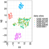
Figure 1: T-SNE plot for the GEO datasets over data sites.

2.3 Evaluation Criteria

To further explain the problem, before discussing any potential solution, we first address the question of how to evaluate model performance, which will help deeper understanding of the problem.

In RFMS, we want to obtain a model that genaralize well for the openbox, curator and hopefully for the lockbox as well, which is a multi-objective problem. Accordingly, the selected model should also be evaluated with method that could take different objectives into consideration.

Dominated hypervolume: A natural criterion is to measure the Dominated Hypervolume[2] of the model performance on the outbag part of openbox and curator site, as well as the lockbox, as in Equation (1)

$$J^{hv}(\phi\mid D_{ob}^{og},\leavevmode\nobreak\ D_{cu}^{og},\leavevmode\nobreak\ D_{lb})=\mathcal{H}\left[f_{ob}^{og},\leavevmode\nobreak\ f_{cu}^{og},\leavevmode\nobreak\ f_{lb}\leavevmode\nobreak\ \right],$$

$$f_{ob}^{og}=\mathcal{F}\left(D_{ob}^{og}\mid\theta=\mathcal{L}(D_{ob}^{ig}\mid\phi)\right),$$

$$f_{cu}^{og}=\mathcal{F}\left(D_{cu}^{og}\mid\theta=\mathcal{L}(D_{ob}^{ig}\mid\phi)\right),$$

$$f_{lb}=\mathcal{F}\left(D_{lb}\mid\theta=\mathcal{L}(D_{ob}^{ig}\mid\phi)\right).$$ (1)

where, $\mathcal{H}$ represent the calculation of the Dominated Hypervolume, and the performance on each data site outbag part is represented as $f_{ob}^{og},\leavevmode\nobreak\ f_{cu}^{og},\leavevmode\nobreak\ f_{lb}$ respectively. Dominated Hypervolume Indicator is also known as Lebesgue Measure or S-Metric which is the hypervolume between a non-dominated front and a reference point. Due to space limit, we invite readers who are not familiar with these multi-objective concepts to refer to the references.

3 Related Work

In this section, we review recent works that has connections with RFMS.

Nested Cross Validation(NCV): NCV [14] uses an outer loop cross validation to safe guard the risk of overfitting during the hyper-parameter tuning process. However, RFMS does not allow cross validation due to the constraint that remote data site can not be used for training.

Federated Learning: Federated learning [24] also consider situations where data is distributed non-i.i.d. across several data sites and possibly unbalanced, but they assume scenarios where data is fully accessible over a huge amounts of data sites compared to a smaller number of data points available at each site. This is different from RFMS, where we consider data can only be accessed through prediction. Moreover, in RFMS, we consider a relatively small amount of data sites with less instances but high dimensional data.

Distribution Shift: Distribution Shift refers to a mismatch in distribution between the data an algorithm was trained on, and data used for model validation or prediction. Detecting and characterizing such shift remains an open problem [42, 29]. In this work, we do not drive deeper in theory of the data shift problem, but provides an empirical study which partially addresses the data shift problem, especially when feature distribution varies across data sites.

Train On Validation: In [36] the authors use parts of the validation dataset for training to generate a stable algorithm. In [41], a progressive resampling process is used. However, both works assume that all the data in question is available for training, which is not possible in RFMS.

Thresholdout Family: [7] showes that differential privacy is deeply associated with model generalization and propose the Thresholdout algorithm to avoid overfitting on the validation set due to repetitive usage. [13] extends the instance wise Thresholdout to AUC measures. However, these methods rely on the i.i.d assumption of data which does not fit our scenario here.

Adaptive Regularization: In [30], the author proposed an alternative update method for model parameter $\theta$ and hyper-parameter $\phi=\lambda$ of a recommendation system[21], where the $\lambda$ is the regularization parameter. In adaptive regularization, the update for the $\lambda$ is based on the ”future” value of performance which is also similar to the EM algorithm update process. However, adaptive regularization only works with gradient based algorithms. Especially, it is only implemented for Factorization Machine in libFM. So in general it does not work for non-gradient based optimization typed machine learning models.

Model Agnostic Meta Learning (MAML): Model Agnostic Meta Learning [10] originates from few shot learning. It aims at adapting to new instances, in which sense is similar to RFMS. However, MAML works only with gradient based method and pre-assumes that the algorithm could see the full subsequent dataset which is not possible in RFMS problem setting.

4 Methods

In this section, we first describe the general RFMS process in 4.1, then in 4.2, we propose how to handle the RFMS process with Bayesian Optimization.

Figure 2: Restrictive Federated Model Selection starting from step $i$

4.1 Restrictive Federated Model Selection

The general process of RFMS is illustrated in Figure 2, which depicts an asynchronous communication process during optimization. At step $i$, based on hyper-parameter $\phi_{i}$, the machine learning model is trained on $D_{ob}$ to get the model parameter $\theta^{i}=\mathcal{L}(D_{ob}\mid\phi^{i})$.

With the same hyper-parameter $\phi_{i}$, a $10$-fold cross validation is carried out on the openbox inbag part $D_{ob}$, which gives us one loss function in Equation (2).

$$J_{i}^{l}(\phi_{i}\mid D_{ob}^{ig})=cv(D_{ob}^{ig}\mid\phi_{i})$$ (2)

where $cv(D_{ob}^{ig}\mid\phi_{i})$ represent the average loss of the cross validation and $J^{l}_{i}$ means local loss at the $i$th step.

Another loss function is obtained by sending the model parameters $\theta^{i}$ to the remote side as shown in Equation (3)

$$J^{r}_{i}(\phi_{i}\mid D_{cu}^{ig})=\mathcal{F}(D_{cu}^{ig}\mid\leavevmode\nobreak\ \theta_{i}=\mathcal{L}(D_{ob}^{ig}\mid\phi_{i}))$$ (3)

Here $J^{r}_{i}$ means loss on the remote curator at the $i$th step.

At the next step, a decision process $\beta$ (see Algorithm 1) based on all historical observations will propose a new hyper-parameter to be tried out for a potential better performance. This process is repeated until budget reached. The process should return the optimal hyper-parameters. The complete procedure is listed in Algorithm 1, where the the decision process $\beta$ to generate the proposal is approximately greedily taking the optimal of a Gaussian Process originated surrogate $\mu(\phi\mid\mathcal{R},\leavevmode\nobreak\ \Phi)$, Expected Improvement [33], for instance. We use $\Phi$ (with an inital design sized $n^{ini}$) to represent the hyper-parameter buffer and $\mathcal{R}$ to represent the corresponding objective(s) buffer.

4.2 Bayesian Optimization and Baselines

Bayesian optimization tries to solve the problem of optimizing (often expensive-to-evaluate) black-box functions by using an internal empirical performance model which learns a surrogate model of the objective function while optimizing it. A widely used application for Bayesian Optimization [16] is the optimization of hyperparameters [33, 1] of machine learning algorithms. Its aim is to find an optimal configuration $\phi^{\star}$ from the feasible region. The choice of hyperparameters for a machine learning model influences the learned model and can thus result in different performances (cf. [31, 28]).

Since the distribution of the data across different data sites is unknown, we propose to treat the model selection approach as a black box optimization problem. Specifically, we use Bayesian Optimization in Algorithm 1 to solve the Restrictive Federated Model Selection problem with the following variants.

Local Single Objective (lso) Bayesian Optimization: In local single objective (lso) Bayesian Optimization, we set objective function as cross validation performance on the local openbox data site, hyper-parameters are tuned based on $J^{lso}(\phi)=J^{l}=cv\left(D_{ob}^{ig}\mid\phi\right)$ where $J^{l}$ is defined in Equation (2).

Federated Single Objective (fso) Bayesian Optimization: In Federated Single Objective Bayesian Optimization, we combine the openbox cross validation aggregated results in Equation (2) and curator performance in Equation (3) linearly as objective function, hyper-parameters are tuned based on

$$J^{fso}(\phi)=\alpha\leavevmode\nobreak\ J^{l}(\phi_{i}\mid D_{ob}^{ig})+\left(1-\alpha\right)J^{r}(\phi_{i}\mid D_{cu}^{ig})$$

$$\alpha\in\left[0,\leavevmode\nobreak\ 1\right].$$ (4)

Specifically, we use $fso2$ to represent $\alpha=0.2$ and $fso8$ to represent $\alpha=0.8$ and so on. Note that $\alpha=1$ corresponds to $lso$. We use different $\alpha$ to check if there is an obvious effects by changing $\alpha$.

Federated Multiobjective Objective ($\mathbf{fmo}$) Bayesian Optimization : Multiobjective Bayesian Optimization [15] optimizes multiple objectives simultaneously, by random linear combination or optimization a S-metric based objective, which avoid deciding which linear combination parameter $\alpha$ to choose. In this work, we use the Parego algorithm [18] to optimize the local objective in Equation (2) and remote objective in Equation (3) jointly.

Random Search Multiobjective (rand_mo): To evaluate whether Bayesian optimization makes sense, we randomly search the hyper-parameter space and select the pareto front [38] as final output, which we call random search multi-objective.

Algorithm 1 RFMS with Bayesian Optimization (RFMS-BO)

1:procedure RFMS-BO $\triangleright$ data site notation here refer to the inbag part

2:     $\Phi_{1:n^{ini}}=\left\{\phi_{1},\ldots,\phi_{n^{ini}}\right\}$ $\triangleright$ initial design as hyper-parameter buffer

3:     $\mathcal{R}_{0}=\emptyset$ $\triangleright$ objective buffer

4:     for $i$ in $1:n^{ini}$, $\phi_{i}$ in $\Phi_{1:n^{ini}}$ do

5:         $J_{i}^{l}(\phi_{i}\mid D_{ob})=cv(D_{ob}\mid\phi_{i})$ $\triangleright$ Cross validation performance aggregation as loss

6:         $\theta_{i}=\mathcal{L}(D_{ob}\mid\phi_{i})$$\triangleright$ training on $D_{ob}$ with $\phi_{i}$

7:         $J^{r}_{i}(\phi_{i}\mid D_{cu},D_{ob})$ = $\mathcal{F}(D_{cu}\mid\theta_{i})$ $\triangleright$ test on curator

8:         $\mathcal{R}_{i}=\mathcal{R}_{i-1}\|\left[J_{i}^{l},J_{i}^{r}\right]$ $\triangleright$ populate objective buffer

9:     end for

10:     fit $\mu(\phi\mid\mathcal{R}_{i},\leavevmode\nobreak\ \Phi_{1:n^{ini}})$ $\triangleright$ train Surrogate Function

11:     $j=i+1$

12:     while budget not reached do

13:         $\phi_{j}=\beta(\mu(\phi\mid\mathcal{R}_{j-1},\leavevmode\nobreak\ \Phi_{1:j-1}))$ $\triangleright$ propose new hyper-parameter

14:         ${\Phi}_{1:j}=\Phi_{1:j-1}\|\left[\phi_{j}\right]$ $\triangleright$ populate hyper-parameter buffer

15:         $J_{j}^{l}(\phi_{j}\mid D_{ob})=cv(D_{ob}\mid\phi_{j})$

16:         $\theta_{j}=\mathcal{L}(D_{ob}\mid\phi_{j})$

17:         $J^{r}_{j}(\phi_{j}\mid D_{cu})$ = $\mathcal{F}(D_{cu}\mid\theta_{j})$

18:         ${\mathcal{R}}_{j}=\mathcal{R}_{j-1}\|\left[J_{j}^{l},\leavevmode\nobreak\ J_{j}^{r}\right]$ $\triangleright$ populate objective buffer

19:         $j\leftarrow j+1$

20:         update $\mu(\phi\mid\mathcal{R}_{j},\leavevmode\nobreak\ \Phi_{1:j})$ $\triangleright$ update surrogate

21:     end while

22:     $i^{*}=\operatorname*{arg\,max}_{i}(\mathcal{R})$

23:     $\{\phi^{*}\}=\Phi_{i*}$

24:     $\{\theta^{*}\}=\mathcal{L}(D_{ob};\phi^{*})$

25:     return $\phi^{*},\theta^{*}$

26:end procedure

4.3 Semi-simulation of Data sites

Publicly available datasets which could fit into the RFMS scenario intrinsically are rare. To get data from a diversified source aside from the Gene Expression Ominbus, we turn to approximate the RFMS scenario by splitting an existing dataset into different parts as if each part sits on a different data site. In practice, we always split an existing dataset into $5$ parts to keep consistence with our GEO datasets.

Since we use real data, but kind of simulate to split the dataset into different data sites to fit into the RFMS scenario, we call this semi-simulation of data sites. We propose the following strategy to semi-simulate the data sites.

Stratified Random Split (SRS): First, split the dataset into two parts according to a factor column. Specifically, we use the target column in a classification dataset. Then, each factor part is randomly split into $5$ buckets. The positive class part got $b^{p}_{1},\ldots,b^{p}_{5}$ and the negative class part got $b^{n}_{1},\ldots,b^{n}_{5}$, where $b^{n}_{i}$ and $b^{p}_{i}$ represent the $i$th bucket in the negative part and positive part respectively. Lastly, sort the buckets in each factor part according to the number of instances and combine the buckets in reversing order to form each data site, i.e., $d_{i}=b^{n}_{s^{n}(i)}\|b^{p}_{s^{p}(6-i)}$, where $d_{i}$ represents the $i$th combined data site, $s^{n}$ and $s^{p}$ are the sorted index vector of each part. We use $\|$ to denote pooling two data buckets.

Dimension Reduction and Clustering(DRC): First, carry out a dimension reduction technique on the dataset like Principal Component Analysis. Then split the dataset into positive class part and negative class part. Cluster each part into $5$ clusters, .i.e. $c^{n}_{1},\leavevmode\nobreak\ \ldots,\leavevmode\nobreak\ c^{n}_{5}$ for the negative class part and $c^{p}_{1},\leavevmode\nobreak\ \ldots,\leavevmode\nobreak\ c^{p}_{5}$ for the positive class part. Sort the clusters with respect to the cluster size in each part and combine them in reversed order to form each data site, i.e., $d_{i}=c^{n}_{s^{n}(i)}\|c^{p}_{s^{p}(6-i)}$, where $d_{i}$ represent the $i$th combined data site, $s^{n}$ and $s^{p}$ are the sorted index vector of each part. We use $\|$ to denote pooling two data together.

We choose Mixture of Gaussian Model (MOG) for the clustering, due to consideration that MOG could also serve as a density estimator.

$$p(X)={{\Sigma}}_{k=1}^{5}c_{k}\mathcal{N}(X|\boldsymbol{\mu}_{k},\boldsymbol{\Sigma}_{k})$$ (5)

In MOG, each cluster is represented by a Gaussian distribution $\mathcal{N}(X|\boldsymbol{\mu}_{k},\boldsymbol{\Sigma}_{k})$ with its own parameters $\boldsymbol{\mu}_{k}$(mean) and $\boldsymbol{\Sigma}_{k}$(covariance), as shown in Equation (5), $c_{k}$ is the mixing coefficient of each cluster. For each of the chosen datasets in Table 2, we model the data distribution as $p(X)$ in Equation(5) and approximately, each cluster resulted data site represent a different distribution. For simplicity, we assume all clusters are with different mean vectors but share the same covariance matrix to assemble a distribution shift. The T-SNE plot is done to the SRS scenario (Figure 5) and the DRC scenario. In DRC, we use PCA as dimension reduction, keeping 10% (Figure 5) and 50% (Figure 5) of the total variance to tell if the reduced dimension makes a big difference in generating an unevenly distributed data sites scenario). From these figures, we do not observe a big difference between different percentage of variance to reserve in PCA, but observe a big difference between SRS and DRC where SRS generates a more evenly distributed data sites, while DRC generates more uneven distributions across different clusters(data sites).

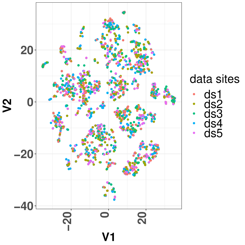
Figure 3: Stratified Random Split (SRS)

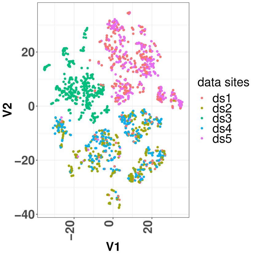
Figure 4: DRC with PCA and keep 10% variance

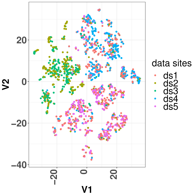
Figure 5: DRC with PCA and keep 50% variance

5 Experiment

5.1 Settings

Since we have selected $5$ datasets from the Gene Expression Ominibus to represent $5$ data sites, we will consider the exemplary problem of $5$ data sites for the remainder of the paper.

In the experiment, one of the $5$ data sites is used as openbox $D_{ob}$, another one as lockbox $D_{lb}$ and the three left over are used as curators $D_{cu}$. We choose to have only one openbox to simulate the scenario, that usually only local data at the current data sites are fully available to the analyst. We choose to have $3$ curators and only $1$ lockbox to simulate the scenario that more data sites want to collaborate with the openbox data site. Curator data site losses are weighted by the size of the each curator data site during optimization. With this strategy, there are in total $5\times 4=20$ combinations of openbox-curator-lockbox on the $5$ datasets. Each openbox and lockbox combination defines one scenario. Each scenario is repeated $10$ times ($10$ replications) where we call each replication one experiment. We sequentially run all RFMS methods, described in Section 4.2, with 3 machine learning algorithms (kernel support vector machine, random forest and elastic net). Thus, we have in total $20\times 10\times 3=600$ experiments given a RFMS problem with $5$ data sites. All Bayesian Optimization procedures share the same initial design of 20 randomly selected configurations, and are then run for another $40$ iterations. Thus in total we have a budget of $60$ evaluations. To have a fair comparison, Random Search use the same number of evaluations.

In order to evaluate our method, we randomly partition openbox and the curator into two parts, namely an inbag part(80%) and an outbag part(20%). Replications mentioned above could average out the random splits and other stochastic factors. We use $D_{ob}^{ig}$ for training a model, and use $D_{cu}^{ig}$ as well as $D_{ob}^{ig}$ for model selection. The outbag parts of openbox and curator are reserved for post-hoc analysis. This allows us to assess, whether our methods overfit in each of the two boxes. Additionally, performance is also recorded on the lockbox site for another aspect of evaluation. We then compare the different methods described in Section 4.2 on the outbag portion of the respective boxes (as noted in 2.1, all data of lockbox belongs to outbag).

5.2 Selection of Dataset for semi-simulation

In order to validate our results on different data sources, we obtain additional data sets from OpenML [39]. As no datasets with an intrinsic splitting mechanism such as the GEO dataset (where each dataset comes from a particular source) are available, we simulate the RFMS scenario according to the strategies described in Section 4.3.

Model generalization becomes more difficult when there are comparatively more features than instances. Therefore, we restrict ourselves to datasets with a relatively high-dimension characteristics: Since we intend to split a dataset into $5$ parts as $5$ data sites, the number or instances in each data site is approximately reduced by $5$ times compared to the original dataset (we rebalanced cluster results which generate too small clusters but adding instances to the smallest cluster from the biggest cluster until the smallest cluster reaches 10 percent of the total number of instances), but the number of features over the number of instances get to be approximately $5$ times of the original ratio, so a $p$ (number of features) over $n$ (number of instances) ratio of more than $0.2$ in the original dataset corresponds to $\frac{p}{n}=1$ in each data site, thus we consider datasets with $\frac{p}{n}$ ratio around $0.2$ to be high-dimensional.

Too few instances is more prone to problems in data resampling processes like cross validation. For example, one fold of the cross validation might contain no instance from the underrepresented class. Thus we do not want too extremely unbalanced classification datasets. In order to have a sufficient amount of data in each of the 5 boxes, we select only data sets with more than $500$ instances. For the purpose of simplicity, we additionally restrict our data set selection to data sets that are $i)$ binary class, $ii)$ do not have missing values. As a result, we use the data sets in Table 2 to provide additional validation of the proposed methods.

Table 2: List of datasets from OpenML

name	n	p	p/n	class ratio
gina agnostic	3468	970	0.28	0.97
Bioresponse	3751	1776	0.47	0.84
$fri\_c4\_500\_100$	500	100	0.2	0.77

5.3 Machine learning algorithms and hyper-parameters

We choose $3$ machine learning algorithms(which we call learner) based on the consideration that the learners should be representative to different mechanisms of various machine learning algorithms. Elastic net logistic regression (implemented in R package $glmnet$ [11]) is a good representative for linear classifier which could deal with high dimensional data(classif.glmnet), thus chosen because according to [35], one should not rule out simple models prematurely. R package $ranger$ [40] implements a random forest(classif.ranger) which is a state of art non-linear learner that has shown outstanding performance. Kernel support vector machine ($ksvm$)(classif.ksvm) implemented in [17], is a nonlinear classifier which could deal with high dimensional data. The hyper-parameters to be optimized with their ranges are shown in Table 3. Hyper-parameter tuning is done with $mlr$[4] and $mlrMBO$[5]. Meaning of hyper-parameters can be found in respective packages.

Table 3: List of Hyperparameters

Classifier	Hyperparameter	Type	Range
glmnet	alpha	numeric	($0$,$1$)
glmnet	s	numeric	($2^{-10}$,$2^{10}$)
ksvm	C	numeric	($2^{-15}$,$2^{15}$)
ksvm	sigma	numeric	($2^{-15}$,$2^{15}$)
random forest	num.trees	integer	(100,5000)
random forest	min.node.size	integer	(1,50)
random forest	sample.fraction	numeric	(0.1,1)

5.4 Results and Discussion

In this section, we compare different candidates of RMFS methods proposed in section 2.3 with respect to their predictive performance. Our aim is to obtain machine learning models, that generalize well across data sites. As an aggregate measure, we choose the dominated hypervolume of the data kept out-of-bag in the openbox $D_{ob}^{og}$, curator $D_{cu}^{og}$ and lockbox $D_{lb}$ respectively as shown in Equation (1). We consider the average performance on the curators for calculating the hypervolume. Lockbox data measures how our methods generalize to sub-populations not considered at all during the training and model selection process. Using hypervolume results in a comprehensive overview of them.

5.4.1 Results on the GEO datasets

As shown in Figure 7, we compare the mean dominated hypervolume from Equation (1) of 3 machine learning algorithms (corresponding to the 3 panels in the plot) and several RFMS methods. We aggregate over $10$ replications and $20$ combinations of possible openbox-lockbox combinations.

From Figure 7, we can observe that $lso$ performs the worst among other candidates, showing that in the RFMS scenario, solely tuning hyper-parameters on the local openbox data site will usually not lead to a model that generalizes well across data sites, which is in accordance with intuition. The other candidates methods including fmo  and several fso  variants, that predicting on the data of the curator and using this performance as a feedback performs better, showing that the feedback could help in arriving at models which generalize better. However, the considered Bayesian Optimization approaches do not overrate the multi-objective random search rand_mo, nor do we observe any effect of changing $\alpha$ in the performance of fso .

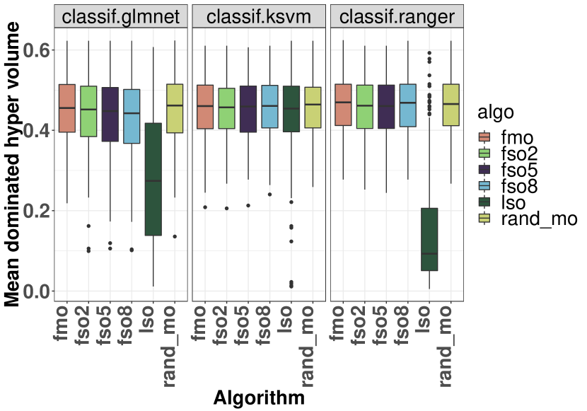
Figure 6: Dominated hypervolume on GEO datasets

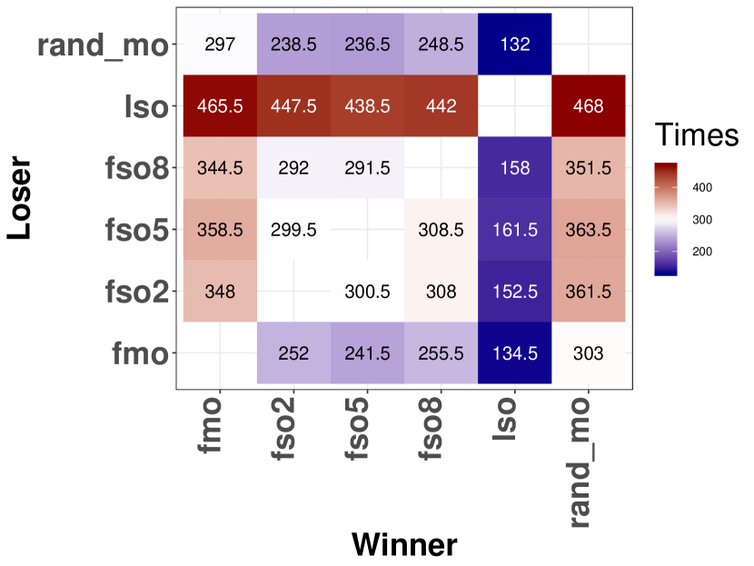
Figure 7: Comparison of wins and losses on GEO dataset

In order to make a more precise comparison, we compare the pairwise wins and losses of all the RFMS methods in terms of dominated hypervolume. For each experiment, we build a $0-1$ matrix to compare the win and loss of each algorithm pair (when method A is compared against method B, we take 0 for loss, 1 for win, and $0.5$ for tie) and aggregate the matrix across all $600$ experiments. Results are shown in Figure 7, where the horizontal axis corresponds to winners and the vertical axis correspond to losers. The elements in the matrix correspond to how many times the winner has won against the loser. It is easily observable that both bi-criteria methods (fmo  and rand_mo) are slightly better than other candidates, as they win more than half of the experiments.

5.4.2 Results on the semi-simulated RFMS scenario

To avoid single dataset bias, we also analyze how the same algorithms compare under our semi-simulated RFMS scenario described in section 4.3 over data of various sources.

Dimension Reduction and Clustering (DRC): We first simulate the RFMS scenario with DRC explained in section 4.3, which could result in a situation that data from different data sites are differently distributed, where we keep 10 percent variance in the PCA step.

Figure 9 shows the dominated hypervolume by aggregating across all the datasets in Table 2. Compared to Figure 7, it is more obvious here that the multi-objective methods work better than the single objective Bayesian optimization methods. In Figure 9, we have the Winner-vs-Loser plot for the aggregated results on the OpenML datasets listed in Table 2, where the multi-objective candidates outperform the rest by a large margin. Furthermore, fmo  wins rand_mo  by a considerable margin, giving confidence that Bayesian Optimization make a difference compared to random search.

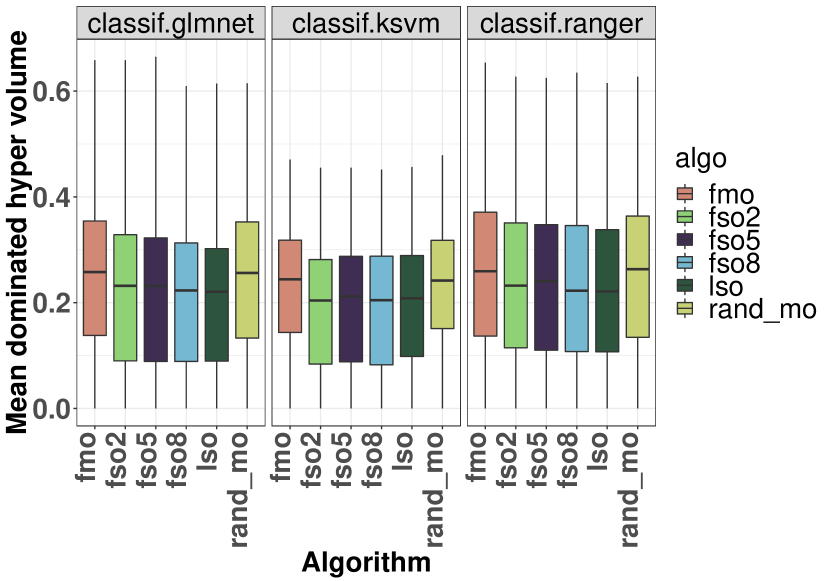
Figure 8: Aggregated mean dominated hypervolume under DRC scenarios obtained over OpenML datasets

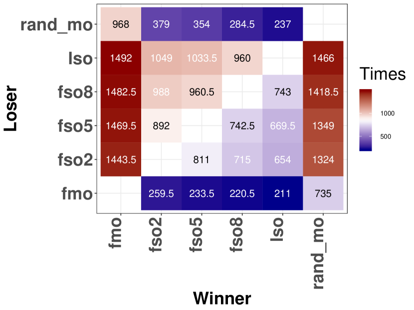
Figure 9: Aggregated wins and losses on the DRC scenarios obtained over OpenML datasets

Stratified Random Split (SRS): To answer the question if a different data splitting technique affects the comparison, we use the stratified technique described in section 4.3 which corresponds to the situation that data being more evenly distributed across data sites. Figure 11 shows the hypervolume plot, from which we can still observe the pattern that the multi-objective candidates perform better in terms of hypervolume, while compared to Figure 9, all methods show increased performance under this evenly distributed data scenario across data sites, possibly due to the bonus of evenly distributed data scenario. In Figure 11, we compare the wins and losses for each pair of candidates, where in this case, the fmo  wins rand_mo  by a larger margin, maybe because the SRS generate a simpler RFMS scenario for the Bayesian Optimization.

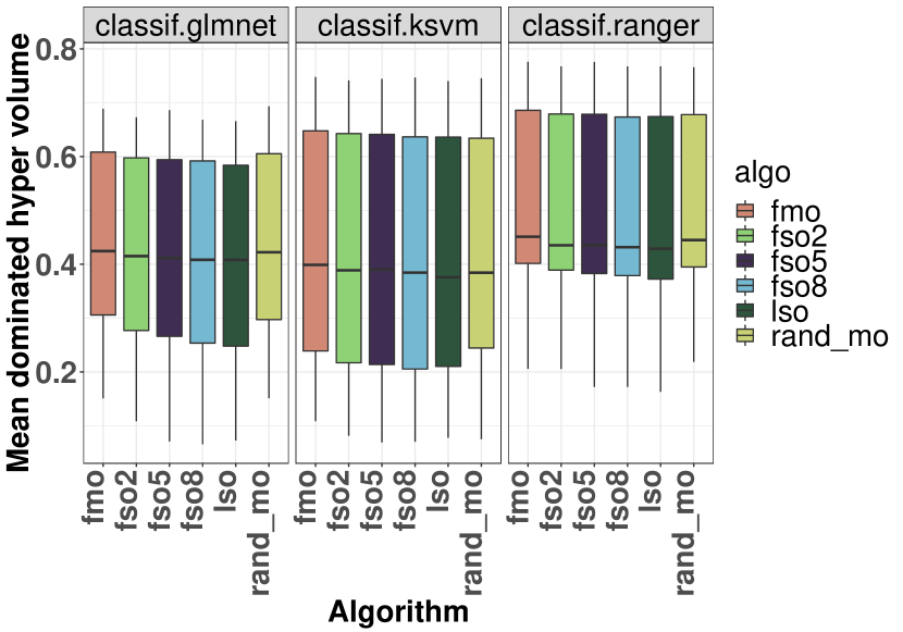
Figure 10: Aggregated mean dominated hyper-volume under SRS scenario obtained over OpenML datasets

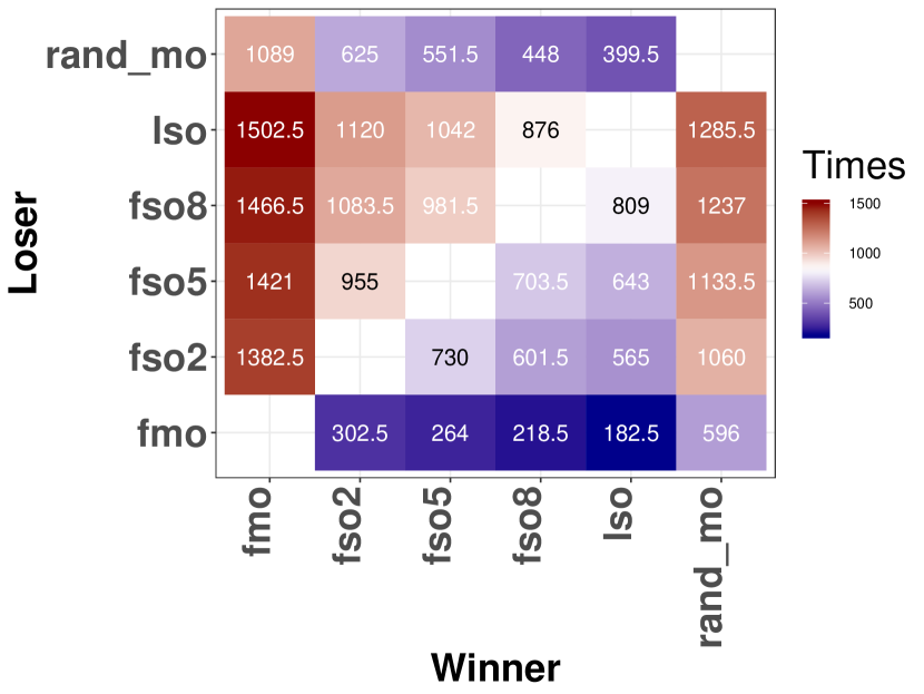
Figure 11: Aggregated wins and losses over SRS scenario obtained over OpenML datasets

Since close or even identical predicative performance values on a problem can occur for varying machine learning hyperparameters, when the predicative performance is used as the target for Gaussian Process regression, it can create numerical difficulties, so hyperparameter tuning might fail for a particular algorithm, even though we use a nugget value of $1e-6$. Therefore, to get fair comparison, all algorithms are run sequentially over a problem on the same computing node. Only those experiments with all algorithms finished are used for analysis, where in practice, we only get neglectable number of experiments (around 100 out of 1800 experiments, which is 5 percent) within which at least one algorithm is not finished, see Figure 9 and Figure 11. The Winner-vs-Loser plots are more effective than carrying out statistical test.

6 Summary

We introduce a novel learning scenario, Restrictive Federated Model Selection (RFMS), which could play an important role in clinical research, where privacy sensitive immobile high dimensional data is differently distributed among various data sites, in which case federated learning is not applicable due to a lack of access to data from all data sites to be used for training. RFMS is a model selection process in this scenario, with the aim to obtain a model that generalizes comparably well across data sites with potential different distributions. Compared to Federated Learning, RFMS can be carried out in an asynchronous fashion, which is not communication hungry compared to standard federated learning and much easier to be deployed. Additionally, the amount of information that needs to be transferred for each query is comparatively small which takes less efforts to be deployed.

As an initial investigation, we compare various methods for model selection and hyper-parameter tuning using Bayesian Optimization. Empirical results from various data sources indicate that Federated Multi-objective Bayesian Optimization compares favorably against other single objective candidates as well as multi-objective random search, in terms of better generalization across data sites.

References

- [1] Bergstra, J.S., Bardenet, R., Bengio, Y., Kégl, B.: Algorithms for hyper-parameter optimization. In: Advances in neural information processing systems, pp. 2546–2554 (2011)
- [2] Beume, N., Rudolph, G.: Faster s-metric calculation by considering dominated hypervolume as klee’s measure problem. Universitätsbibliothek Dortmund (2006)
- [3] Bhowmick, A., Duchi, J., Freudiger, J., Kapoor, G., Rogers, R.: Protection Against Reconstruction and Its Applications in Private Federated Learning. arXiv:1812.00984 (2018)
- [4] Bischl, B., Lang, M., Kotthoff, L., Schiffner, J., Richter, J., Studerus, E., Casalicchio, G., Jones, Z.M.: mlr: Machine learning in r. The Journal of Machine Learning Research 17(1), 5938–5942 (2016)
- [5] Bischl, B., Richter, J., Bossek, J., Horn, D., Thomas, J., Lang, M.: mlrmbo: A modular framework for model-based optimization of expensive black-box functions. arXiv preprint arXiv:1703.03373 (2017)
- [6] Cawley, G.C., Talbot, N.L.: On over-fitting in model selection and subsequent selection bias in performance evaluation. Journal of Machine Learning Research 11(Jul), 2079–2107 (2010)
- [7] Dwork, C., Feldman, V., Hardt, M., Pitassi, T., Reingold, O., Roth, A.: Guilt-free data reuse. Communications of the ACM 60(4), 86–93 (2017)
- [8] Edgar, R., Domrachev, M., Lash, A.E.: Gene expression omnibus: Ncbi gene expression and hybridization array data repository. Nucleic acids research 30(1), 207–210 (2002)
- [9] Elder, S.: Bayesian adaptive data analysis guarantees from subgaussianity. arXiv preprint arXiv:1611.00065 (2016)
- [10] Finn, C., Abbeel, P., Levine, S.: Model-agnostic meta-learning for fast adaptation of deep networks. arXiv preprint arXiv:1703.03400 (2017)
- [11] Friedman, J., Hastie, T., Tibshirani, R.: glmnet: Lasso and elastic-net regularized generalized linear models. R package version 1(4) (2009)
- [12] Geyer, R.C., Klein, T., Nabi, M.: Differentially private federated learning: A client level perspective. arXiv preprint arXiv:1712.07557 (2017)
- [13] Gossmann, A., Pezeshk, A., Sahiner, B.: Test data reuse for evaluation of adaptive machine learning algorithms: over-fitting to a fixed’test’dataset and a potential solution. In: Medical Imaging 2018: Image Perception, Observer Performance, and Technology Assessment, vol. 10577, p. 105770K. International Society for Optics and Photonics (2018)
- [14] Guyon, I., Saffari, A., Dror, G., Cawley, G.: Model selection: Beyond the bayesian/frequentist divide. Journal of Machine Learning Research 11(Jan), 61–87 (2010)
- [15] Horn, D., Dagge, M., Sun, X., Bischl, B.: First investigations on noisy model-based multi-objective optimization. In: International Conference on Evolutionary Multi-Criterion Optimization, pp. 298–313. Springer (2017)
- [16] Jones, D.R., Schonlau, M., Welch, W.J.: Efficient global optimization of expensive black-box functions. Journal of Global optimization 13(4), 455–492 (1998)
- [17] Karatzoglou, A., Smola, A., Hornik, K., Zeileis, A.: kernlab-an s4 package for kernel methods in r. Journal of statistical software 11(9), 1–20 (2004)
- [18] Knowles, J.: Parego: a hybrid algorithm with on-line landscape approximation for expensive multiobjective optimization problems. IEEE Transactions on Evolutionary Computation 10, 50–66 (2006)
- [19] Konecnỳ, J., McMahan, H.B., Ramage, D., Richtárik, P.: Federated optimization: Distributed machine learning for on-device intelligence. arXiv preprint arXiv:1610.02527 (2016)
- [20] Konečnỳ, J., McMahan, H.B., Yu, F.X., Richtárik, P., Suresh, A.T., Bacon, D.: Federated learning: Strategies for improving communication efficiency. arXiv preprint arXiv:1610.05492 (2016)
- [21] Kushwaha, N., Sun, X., Singh, B., Vyas, O.: A lesson learned from pmf based approach for semantic recommender system. Journal of Intelligent Information Systems 50(3), 441–453 (2018)
- [22] Maaten, L.v.d., Hinton, G.: Visualizing data using t-sne. Journal of machine learning research 9(Nov), 2579–2605 (2008)
- [23] McCall, M.N., Bolstad, B.M., Irizarry, R.A.: Frozen robust multiarray analysis (frma). Biostatistics 11(2), 242–253 (2010)
- [24] McMahan, H.B., Moore, E., Ramage, D., Hampson, S., y Arcas, B.A.: Communication-efficient learning of deep networks from decentralized data. In: AISTATS (2017)
- [25] McMahan, H.B., Moore, E., Ramage, D., Hampson, S., et al.: Communication-efficient learning of deep networks from decentralized data. arXiv preprint arXiv:1602.05629 (2016)
- [26] Melis, L.: Building and evaluating privacy-preserving data processing systems. Ph.D. thesis, UCL (University College London) (2018)
- [27] Melis, L., Song, C., De Cristofaro, E., Shmatikov, V.: Inference attacks against collaborative learning. arXiv preprint arXiv:1805.04049 (2018)
- [28] Probst, P., Bischl, B., Boulesteix, A.L.: Tunability: Importance of hyperparameters of machine learning algorithms. arXiv preprint arXiv:1802.09596 (2018)
- [29] Rabanser, S., Günnemann, S., Lipton, Z.C.: Failing loudly: An empirical study of methods for detecting dataset shift. arXiv preprint arXiv:1810.11953 (2018)
- [30] Rendle, S.: Learning recommender systems with adaptive regularization. In: Proceedings of the fifth ACM international conference on Web search and data mining, pp. 133–142. ACM (2012)
- [31] van Rijn, J.N., Hutter, F.: Hyperparameter importance across datasets. In: Proceedings of the 24th ACM SIGKDD International Conference on Knowledge Discovery & Data Mining, pp. 2367–2376. ACM (2018)
- [32] Shokri, R., Stronati, M., Song, C., Shmatikov, V.: Membership inference attacks against machine learning models. In: 2017 IEEE Symposium on Security and Privacy (SP), pp. 3–18 (2017). 10.1109/SP.2017.41
- [33] Snoek, J., Larochelle, H., Adams, R.P.: Practical bayesian optimization of machine learning algorithms. In: Advances in neural information processing systems, pp. 2951–2959 (2012)
- [34] Snoek, J., Rippel, O., Swersky, K., Kiros, R., Satish, N., Sundaram, N., Patwary, M., Prabhat, M., Adams, R.: Scalable bayesian optimization using deep neural networks. In: International Conference on Machine Learning, pp. 2171–2180 (2015)
- [35] Strang, B., van der Putten, P., van Rijn, J.N., Hutter, F.: Don’t rule out simple models prematurely: A large scale benchmark comparing linear and non-linear classifiers in openml. In: International Symposium on Intelligent Data Analysis, pp. 303–315. Springer (2018)
- [36] Tennenholtz, G., Zahavy, T., Mannor, S.: Train on validation: Squeezing the data lemon. arXiv preprint arXiv:1802.05846 (2018)
- [37] Truex, S., Baracaldo, N., Anwar, A., Steinke, T., Ludwig, H., Zhang, R.: A hybrid approach to privacy-preserving federated learning. arXiv preprint arXiv:1812.03224 (2018)
- [38] Van Veldhuizen, D.A., Lamont, G.B.: Evolutionary computation and convergence to a pareto front. In: Late breaking papers at the genetic programming 1998 conference, pp. 221–228 (1998)
- [39] Vanschoren, J., van Rijn, J.N., Bischl, B., Torgo, L.: OpenML: networked science in machine learning. ACM SIGKDD Explorations Newsletter 15(2), 49–60 (2014)
- [40] Wright, M.N., Ziegler, A.: Ranger: a fast implementation of random forests for high dimensional data in c++ and r. arXiv preprint arXiv:1508.04409 (2015)
- [41] Zeng, X., Luo, G.: Progressive sampling-based bayesian optimization for efficient and automatic machine learning model selection. Health information science and systems 5(1), 2 (2017)
- [42] Zhang, K., Schölkopf, B., Muandet, K., Wang, Z.: Domain adaptation under target and conditional shift. In: International Conference on Machine Learning, pp. 819–827 (2013)
- [43] Zhao, Y., Li, M., Lai, L., Suda, N., Civin, D., Chandra, V.: Federated learning with non-iid data. CoRR abs/1806.00582 (2018)