Passage through a sub-diffusing geometrical bottleneck

Abstract

The usual Kramers theory of reaction rates in condensed media predict the rate to have an inverse dependence on the viscosity of the medium, $\eta$. However, experiments on ligand binding to proteins, performed long ago, showed the rate to have $\eta^{-\nu}$ dependence, with $\nu$ in the range $0.4-0.8$. Zwanzig (Journal of Chemical Physics 97, 3587 (1992)) suggested a model, in which the ligand has to pass through a fluctuating opening to reach the binding site. This fluctuating gate model predicted the rate to be proportional to $\eta^{-1/2}$. More recently, experiments performed by Xie et. al. (Physical Review Letters 93, 1 (2004)) showed that the distance between two groups in a protein undergoes not normal diffusion, but subdiffusion. Hence in this paper, we suggest and solve a generalisation of the Zwanzig model, viz., passage through an opening, whose size undergoes sub-diffusion. Our solution shows that the rate is proportional to $\eta^{-\nu}$ with $\nu$ in the range $0.5-1$, and hence the sub-diffusion model can explain the experimental observations.

I Introduction

Simple, exactly solvable models of chemical reaction dynamics are very useful, as they give very valuable insights into the process. Among the very few such models is the one due to Zwanzig (Zwanzig, 1992), for the passage of a ligand molecule through a fluctuating bottleneck. Many authors have suggested similar models for the removal of a steric constraint by fluctuations, for molecular rotation in liquids and glasses (Glarum, 1960; Hunt and Powles, 1966; Bordewijk, 1975; Frobose and Jackle, 1986; Klafter and Blumen, 1985). The model of Zwanzig is for the passage of a ligand to a binding site that is buried deep inside a cavity within a protein. It assumes that the rate of binding is proportional to the area of the opening, which undergoes time dependent fluctuations. In general, the predictions of the model are in agreement with the experiments. The concentration of the ligand initially decays non-exponentialy, but changes over to exponential at long times. Taking the time scale of decay of the fluctuations of the opening as proportional to the viscosity $\eta$ of the medium, the model predicted that the rate constant for long term decay is $\propto$ $\eta^{-1/2}$. In comparison, the Kramers theory of activated processes leads to a rate proportional to $\eta^{-1}$. The experiments of Beece et al. (Beece et al., 1980) on the viscosity dependence of the rate, found an inverse fractional dependence of the form $\eta^{-\nu}$, in agreement with the Zwanzig theory. However, the value of $\nu$ was in the range $0.4-0.8$, prompting the study by Wang and Wolynes (Wang and Wolynes, 1993), of its extension to a non-Markovian model, in which the relaxation of the opening was taken to be a stretched exponential. They used the path integral technique to obtain the exact solution in the long time limit. Their model leads to $\nu$ values that are strictly less than $1/2$. Over the years, there have been a few more investigations into this rather old problem (Eizenberg and Klafter, 1996; Berezhkovskii et al., 1998; Seki and Tachiya, 2000; Berezhkovskii and Shvartsman, 2016). Of particular interest is the paper by Bicout and Szabo Bicout and Szabo (1998) who obtained general results for the rate in the case where the opening undergoes non-Markovian fluctuations. Even though most of these papers were published long ago, we have not been able to find in the literature, a simple analytically solvable model that accounts for all the experimental results. It is the aim of this paper to provide such a simple model, based on information from the very interesting experiments (Yang et al., 2003; Kou and Xie, 2004; Min et al., 2005; Min and Xie, 2006), that have become available since these original investigations.

Most of the above investigations assume the radius of the opening to undergo diffusive motion in a harmonic potential. That is, it is an Ornstein-Uhlenbeck process, with an exponential correlation function. The major exception to this is the work of Wang and Wolynes (Wang and Wolynes, 1993), which models the correlation as a stretched exponential, as well as that of Bicout and Szabo Bicout and Szabo (1998). In an elegant set of papers, the group of Xie (Yang et al., 2003; Kou and Xie, 2004; Min et al., 2005; Min and Xie, 2006) investigated the dynamics of the distance between two units in a protein, that are not directly bonded. Using single molecule fluorescence as a probe of the distance $x$, they showed that $x$ undergoes subdiffusion, in which its mean square displacement is proportional to $(time)^{\beta}$ with $\beta<1$. Further, they also showed that the units may be modelled as being held together by a harmonic spring, and that their motion is well described by the equation for a subdiffusing Brownian oscillator (see Eq. (5)), given in Section I.

Interestingly, the problem of a “quadratic sink representing a gate whose dynamics is diffusive” is of interest in other areas of chemical physics too. One example is the recent observation of “anomalous yet Brownian” diffusion in crowded rearranging media, where the probability distribution of the displacement at short times is found to be exponential, rather than the expected Gaussian Wang et al. (2009). It crosses over to being Gaussian at long times. Interestingly, the mean square displacement at all times is proportional to the time. This has been explained as resulting from the rearrangement of the medium, leading to time dependent random changes in the diffusion coefficient of the particle Chubynsky and Slater (2014); Metzler (2017). We have suggested a model for calculating the probability distribution of the position of such a particle. In this model, the probability distribution is the Fourier transform of the survival probability of a particle undergoing Brownian motion (Jain and Sebastian, 2016a, b, 2017a, 2017b, 2017c). Another interesting study is the “Fluctating Bottleneck model” for the passage of a DNA molecule through the $\alpha$-hemolysin pore by Bian et al. (Bian et al., 2015; Chatterjee and Cherayil, 2010), who found an approximate solution to the model, using the Wilhemski-Fixman approach. It is of interest to note that our study provides an exact solution to this model, though in this paper, we do not discuss our model in this context.

II The fluctuating Gate Model

The process that we study is shown schematically in Fig. 1.

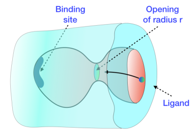
Figure 1: Schematic picture of gating

In order to bind to the site that is inside the cavity, the ligand has to pass through a gate which is modelled as a circular opening of radius $r$. The survival probability of the ligand at the time $t$, $S(t)$ is assumed to obey the equation

$$\frac{dS(t)}{dt}=-K(r)S(t).$$ (1)

Zwanzig (Zwanzig, 1992) takes the rate of passage of the ligand to be proportional to $\pi r^{2}$, the area of the circular gate so that

$$K(r)=kr^{2}.$$ (2)

The radius of the pore undergoes thermal fluctuations, obeying the equation for overdamped motion

$$\zeta\frac{dr}{dt}=-m\omega_{0}^{2}r+\sqrt{2\zeta k_{B}T}\xi(t),$$ (3)

where $m$ is the “mass” associated with the fluctating co-ordinate, and $\frac{\zeta}{m\omega_{0}^{2}}$ is its time of relaxation. $\xi(t)$ is Gaussian white noise with mean zero with $\left\langle\xi(t)\xi(t^{\prime})\right\rangle=\delta(t-t^{\prime})$ and $T$ is the temperature. $\zeta$ is the friction coefficient and is directly proportional to the viscosity $\eta$ of the medium. (Note that our notation is different from that of Zwanzig. Zwanzig’s $\theta$ and $\lambda$ are related to our constants by $\lambda=m\omega_{0}^{2}/\zeta$ and $\theta=\frac{k_{B}T}{m\omega_{0}^{2}}).$ The quantity of interest is $\left\langle S(t)\right\rangle=\int_{0}^{\infty}dr\bar{S}(r,t)$, where the noise averaged concentration $\bar{S}(r,t)$ obeys the reaction-diffusion equation with a sink term that is quadratic in the co-ordinate $r$:

$$\frac{\partial\bar{S}}{\partial t}=-kr^{2}\bar{S}+\frac{k_{B}T}{\zeta}\frac{\partial}{\partial r}\left(\frac{\partial\bar{S}}{\partial r}+\frac{m\omega_{0}^{2}}{k_{B}T}r\bar{S}\right).$$ (4)

Assuming that $\bar{S}$ has the equilibrium distribution at the initial time $t=0$, the instant at which the sink term in Eq. (4) is switched on, this can be solved exactly. The solution leads to the following results: (1) The decay of $\left\langle S(t)\right\rangle$ is multi-exponential. (2) At short times, $\bar{S}(t)=1-k\frac{k_{B}T}{m\omega_{0}^{2}}t+O(t^{2})$. (3) For long times, the decay is single exponential with a rate constant equal to $k_{eff}=\frac{1}{2}\left(\sqrt{4\frac{k_{B}T}{\zeta}k+(\frac{m\omega_{0}^{2}}{\zeta})^{2}}-\frac{m\omega_{0}^{2}}{\zeta}\right).$ For large $\frac{m\omega_{0}^{2}}{\zeta}$, one gets $k_{eff}\approx(k\frac{k_{B}T}{\zeta})^{1/2}$. As $\zeta$ is proportional to $\eta,$ we get $k_{eff}\propto\eta^{-1/2}$, in agreement with experimental observations of Beece et. al. (Beece et al., 1980), of an $\eta^{-\nu}$ dependence with $\nu$ in the range $0.4-0.8.$ The deviation of the predicted value of $\nu$ from the observed, shows that the model of Zwanzig can be considered only as a starting point. This prompted Wang and Wolynes (WW) (Wang and Wolynes, 1993, 1994) to consider a model in which correlation $\left\langle r(t)r(t^{\prime})\right\rangle$ has the form of a stretched exponential given by $\theta\exp\left[-\left(\lambda|t-t^{\prime}|\right)^{\beta}\right]$, with $\beta\leq 1$. Note that $\beta=1$ would be the case considerd by Zwanzig (Zwanzig, 1992), and $\beta\leq 1$ is a more general case of fluctuations, observed in biomolecules and glasses. In this more general case, Wang and Wolynes (Wang and Wolynes, 1993) found an exact expression for the rate constant $k_{eff}$, as a combination of Hypergeometric functions. For $\beta=1$, their result reduces to that of Zwanzig. For $\beta\neq 1$, they obtained an approximation to their result, which predicted a rate proportional to $\eta^{-\beta/(1+\beta)}.$ As $\beta\leq 1,$ this approximate result gives $\nu\leq 1/2$. They conclude that the inclusion of direct coupling of the reaction co-ordinate with the viscous medium is required to have better agreement with experiment. Bicout and Szabo Bicout and Szabo (1998) considered the case where the bottleneck undergoes non-Markovian fluctuations. They obtained analytical expressions for the rate, similar to that of Wang and Wolynes. Their calculations Bicout and Szabo (1998) showed the “Kramers turnover” behaviour as function of $\eta$, but did not give an explanation of the value of $\nu$ that was reported experimentally.

Thanks to the advances in single molecule experiments, we now have more information on the fluctuations of the distance between two sub-units in a protein. Yang et. al. (Yang et al., 2003) showed that the distance $x$ between the Flavin mononucleotide (FMN) and the Flavin adenine dinucleotide (FAD) in the protein flavin reductase, isolated from Escheria coli, undergoes subdiffusive motion. Its dynamics is well described by the equation for a subdiffusive Brownian oscillator (SBO),

$$\zeta\int_{-\infty}^{t}dt^{\prime}K_{\alpha}(t-t^{\prime})\dot{x}(t^{\prime})=-m\omega_{0}^{2}x(t)+\sqrt{2k_{B}T\zeta}\xi^{\alpha}(t).$$ (5)

In the above, $\xi^{\alpha}(t)$ is the fractional Gaussian noise (fGn) having the correlation function

$$\left\langle\xi^{\alpha}(t)\xi^{\alpha}(s)\right\rangle=K_{\alpha}(t-s),$$ (6)

where

$$K_{\alpha}(t-s)=(\alpha+1)\alpha\left|t-s\right|^{\alpha-1}+2(\alpha+1)|t-s|^{\alpha}\delta(t-s),$$ (7)

with $0\leq\alpha<1$. $\alpha=0$ corresponds to the usual Gaussian white noise. Note that Kou and Xie (Kou and Xie, 2004) use the parameter $H$ instead of our $\alpha$ and the two are related by $H=(\alpha+1)/2.$ The use of such an equation is also justified by the analysis of Dua and Adhikari (Dua and Adhikari, 2011). These studies suggest strongly that a very simple model for the passage through a gate is to assume that the dynamics of the gate is sub-diffusive. We discuss this model in the next Section. The model, as will be seen in Section 30, predict a value of $\nu\geq 1/2$, in agreement with the experimental observations.

III Subdiffusive Gating

III.1 The Model

The instantaneous state of the opening may be described by the position vector $\boldsymbol{r}=x\hat{\boldsymbol{i}}+y\hat{\boldsymbol{j}}$, of a point on its circumference, with the origin of the co-ordinates located at the center of the pore. The area of the opening is $\pi r^{2}=\pi\boldsymbol{r}^{2}=\pi\left(x^{2}+y^{2}\right)$. We take $\boldsymbol{r}$ to obey the subdiffusion equation

$$\zeta\int_{-\infty}^{t}dt^{\prime}K_{\alpha}(t-t^{\prime})\frac{d\boldsymbol{r}(t^{\prime})}{dt^{\prime}}=-m\omega_{0}^{2}\boldsymbol{r}(t)+\sqrt{2k_{B}T\zeta}\boldsymbol{\xi}^{\alpha}(t).$$ (8)

$\boldsymbol{\xi}^{\alpha}(t)=\xi^{\alpha}_{x}(t)\hat{\boldsymbol{i}}+\xi^{\alpha}_{y}(t)\hat{\boldsymbol{j}}$, where $\xi^{\alpha}_{i}(t)$ with $i=x,y$, are both white noises having the correlation functions $\left<\xi_{i}^{\alpha}(t)\xi_{j}^{\alpha}(s)\right>=\delta_{ij}K_{\alpha}(t-s)$. For more details on this equation and its application to single molecule experiments, we refer the reader to the articles by Kou (Kou, 2008; Qian and Kou, 2014). One can easily calculate the correlation function,

$$C_{\alpha}(t,t^{\prime})=\left\langle x(t)x(t^{\prime})\right\rangle=\left\langle y(t)y(t^{\prime})\right\rangle=\frac{k_{B}T}{m\omega_{0}^{2}}E_{1-\alpha}\left(-(|t-t^{\prime}|/\tau)^{1-\alpha}\right)$$ (9)

with

$$\tau=\left(\frac{\zeta\Gamma(\alpha+2)}{m\omega_{0}^{2}}\right)^{1/(1-\alpha)}$$ (10)

and $E_{a}(z)$ is the Mittag-Leffler function, defined by $E_{a}(z)=\sum_{k=0}^{\infty}\frac{z^{k}}{\Gamma(ak+1)}$. Also,

$$\left\langle x(t)y(t^{\prime})\right\rangle=0.$$ (11)

It is to be noted that the processes $x(t)$ and $y(t)$ are stationary. Hence we have $C_{\alpha}(t,t^{\prime})=C_{\alpha}(t-t^{\prime}).$ As a result of all the above,

$$\langle\boldsymbol{r}(t)\cdot\boldsymbol{r}(t^{\prime})\rangle=2C_{\alpha}(t-t^{\prime}).$$ (12)

In the following, we will also need the Fourier cosine transform of $C_{\alpha}(t)$, defined by

$$\tilde{C_{\alpha}}(\omega) =\int_{0}^{\infty}dt\cos\left(t\omega\right)C_{\alpha}(t)=\int_{0}^{\infty}dt\cos\left(t\omega\right)\frac{k_{B}T}{m\omega_{0}^{2}}E_{1-\alpha}\left(-(|t-t^{\prime}|/\tau)^{1-\alpha}\right)$$ (13)

$$=\frac{k_{B}T}{m\omega_{0}^{2}}\;\frac{\tau\cos\left(\frac{\pi\alpha}{2}\right)(\tau w)^{-\alpha}}{1+(\tau w)^{2-2\alpha}+2\sin\left(\frac{\pi\alpha}{2}\right)(\tau w)^{1-\alpha}}.$$ (14)

See the review by Kou Kou (2008) for the derivation of the correlation function.

III.2 Survival probability

On solving Eq. (1) using Eq. (2), we get the survival probability of the ligand after a time $t$ to be

$$\left\langle S(t)\right\rangle=\left\langle\exp\left(-k\int_{0}^{t}ds\boldsymbol{r}^{2}(s)\right)\right\rangle,$$ (15)

where the average $\left\langle...\right\rangle$ is over all possible realizations of $\boldsymbol{r}(s)$. We now introduce $\boldsymbol{\eta}(t)=\eta_{x}(t)\hat{\boldsymbol{i}}+\eta_{y}(t)\hat{\boldsymbol{j}},$ where $\eta_{i}(t)$ with $i=x,y$ are both Gaussian white noises, having mean zero and correlation $\left\langle\eta_{i}(t)\eta_{j}(t^{\prime})\right\rangle=\delta_{ij}\delta(t-t^{\prime})$. Using the result,

$$\int D\boldsymbol{\eta}(s)\exp\left(-\int_{0}^{t}ds\boldsymbol{\eta}^{2}(s)+2i\sqrt{k}\int_{0}^{t}ds\boldsymbol{r}(s)\cdot\boldsymbol{\eta}(s)\right)=\exp\left(-k\int_{0}^{t}ds\boldsymbol{r}^{2}(s)\right),$$

it is possible to rewrite Eq. (15) as

$$\left\langle S(t)\right\rangle=\int D\boldsymbol{\eta}(s)\left\langle\exp\left(-\int_{0}^{t}ds\boldsymbol{\eta}^{2}(s)+2i\sqrt{k}\int_{0}^{t}ds\boldsymbol{r}(s)\cdot\boldsymbol{\eta}(s)\right)\right\rangle,$$

where the functional integral $\int D\boldsymbol{\eta}(s)$ is over all possible realizations of $\boldsymbol{\eta}(s)$. As $\boldsymbol{r}(s)$ is a Gaussian stochastic process with mean zero, the average over it is easily performed to get (see the book by Chaichian and Demichev Chaichian and Demichev (2001) or the book by Zinn-Justin Zinn-Justin (2005), for an introduction to functional integrals and their applications).

$$\left\langle S(t)\right\rangle = \int D\boldsymbol{\eta}(s)\exp\left(-\int_{0}^{t}ds\boldsymbol{\eta}^{2}(s)-2k\int_{0}^{t}ds^{\prime}\int_{0}^{t}ds\boldsymbol{\eta}(s)\cdot\left\langle\boldsymbol{r}(s)\;\boldsymbol{r}(s^{\prime})\right\rangle\cdot\boldsymbol{\eta}(s^{\prime})\right)$$ (16)

The tensorial average $\left\langle\boldsymbol{r}(s)\;\boldsymbol{r}(s^{\prime})\right\rangle$ is to be performed over all realisations of the process $\boldsymbol{r}(s)$. Using Eq. (9) and (11), this may be written as

$$\left\langle S(t)\right\rangle = \int D\boldsymbol{\eta}(s)\exp\left(-\int_{0}^{t}ds\boldsymbol{\eta}^{2}(s)-2k\int_{0}^{t}ds^{\prime}\int_{0}^{t}ds\boldsymbol{\eta}(s)\cdot\boldsymbol{\eta}(s^{\prime})C_{\alpha}(s-s^{\prime})\right).$$ (17)

Noting that $\boldsymbol{\eta}(s)$ is a two dimensional vector, and performing the functional integration over it gives

$$\left\langle S(t)\right\rangle = A\left(\det\left[\delta(s-s^{\prime})+2kC_{\alpha}(s-s^{\prime})\right]\right)^{-1}\hskip 14.22636pt\mbox{with}\hskip 14.22636pts,s^{\prime}\;\in\;(0,t).$$ (18)

In the above, $\delta(s-s^{\prime})+2kC_{\alpha}(s-s^{\prime})$ is the $(s,s^{\prime})^{th}$ element of a functional matrix whose labels $s,s^{\prime}$ are continuous. $A$ is a constant, equal to $\det\left[\delta(s-s^{\prime})\right],$ which is divergent. Note that the value of $\left\langle S(t)\right\rangle$ is the ratio of two divergent quantities and is always finite, as it should be (see below). We use the identity $\det B=\exp\left(Tr\ln B\right),$ where $Tr$ stands for the trace of the matrix, valid for any Hermitian matrix $B,$ to write

$$\left\langle S(t)\right\rangle=A\exp\left(-tr\ln\left[\delta(s-s^{\prime})+2kC_{\alpha}(s-s^{\prime})\right]\right).$$

Expanding the logaritham, and using the condition $\left\langle S(t)\right\rangle|_{k=0}=1,$ we get

$$\left\langle S(t)\right\rangle=\exp\left(\sum_{n=1}^{\infty}(-1)^{n}\frac{(2k)^{n}}{n}Tr\boldsymbol{C}_{\alpha}^{n}\right),$$ (19)

where $\boldsymbol{C}_{\alpha}$ is the matrix with continuous labels $s,s^{\prime}$, defined by $\boldsymbol{C}_{\alpha}(s,s^{\prime})=C_{\alpha}(s-s^{\prime}).$ Equation (19) is our final expression, and we can now analyse it, to get the detailed behavior of the survival probability.

III.3 Short time behavior

For small times, i.e., $t\ll\tau,$ we can approximate $C_{\alpha}(s-s^{\prime})$ by $C_{\alpha}(0).$ Doing this in each term in Eq. (19), noting from Eq. (9) that $C_{\alpha}(0)=\frac{k_{B}T}{m\omega_{0}^{2}}$, and summing the resultant series gives

$$\left\langle S(t)\right\rangle=\left(1+2k\frac{k_{B}T}{m\omega_{0}^{2}}t\right)^{-1}\approx 1-2k\frac{k_{B}T}{m\omega_{0}^{2}}t+O(t^{2}),$$

exactly as in the case of the Zwanzig model. Thus subdiffusion of the gate does not make any difference to the short term behavior of the survival probability.

III.4 An exact expression for numerical evaluation of $\left\langle S(t)\right\rangle$

An exact expression, which may be used for numerical evaluation of the survival probabilty can be obtained by discretisation of the time interval $(0,t)$ into $N$ discrete intervals each of duration $\Delta t$, so that $N\Delta t=t.$ Denoting $s_{j}=(j-1)\Delta t,$ with $j=1,2,3,\ldots N$, and approximating the matrix $\boldsymbol{C}_{\alpha}(s,s^{\prime})$ by the finite dimensional matrix $\boldsymbol{C}_{\alpha;N}$ with matrix elements, $\left(C_{\alpha;N}\right)_{ij}=C_{\alpha}(s_{i}-s_{j})\Delta t$ in each term of the sum in the exponent of Eq. (19) gives

$$\left\langle S(t)\right\rangle=\lim_{N\rightarrow\infty,\Delta t\rightarrow 0,N\Delta t=t}\;\left(\det[\boldsymbol{I+}2k\boldsymbol{C_{\alpha}}_{N}]\right)^{-1},$$

where $\boldsymbol{I}$ is the $N\times N$ identity matrix. The value of $N$ can be chosen sufficiently large to get the survival probability to any desired accuracy.

III.5 Survival probability in the long time limit

One can easily get an approximation for $\left\langle S(t)\right\rangle$ in the long time limit. First we note that the matrix $\boldsymbol{I+}\boldsymbol{C}_{\alpha;N}$ would be the Hamiltonian matrix for a chain of $N$ atoms, in a tight binding model, having one orbital on each atom, with all the diagonal elements equal to $1+2kC_{\alpha}(0)\Delta t$ and the $ij^{th}$ offdiagonal element equal to $2kC_{\alpha}(\Delta t(i-j))\Delta t.$ We also note that $C_{\alpha}(t)$ is a decaying function of $t,$ decreasing like $t^{\alpha-1}$ for large values of $t,$ for $\alpha\neq 0$ (if $\alpha=0,$ then it decays exponentially). In either case, for large values of $t$ one expects that modifying the Hamiltonian matrix by imposing periodic boundary conditions on the chain of atoms will not cause a significant change to its eigenvalues. Once the condition is imposed, the eigenvectors of the matrix are $\phi_{j}$ with its $n^{th}$ element being given by $\phi_{j,n}=\frac{1}{\sqrt{N}}e^{i\frac{2\pi nj}{N}}$, where $j$ varies from $-N/2$ to $N/2+1$ and $n$ varies from $0$ to $(N-1)$. With this, it is easy to calculate the $j^{th}$ eigenvalue of the matrix $\boldsymbol{I+}\boldsymbol{C}_{\alpha;N}$. It is given by

$$\epsilon_{j}=1+2k\Delta t\sum_{n=-N/2+1}^{N/2}C_{\alpha}(n\Delta t)\,\exp\left(i\frac{2\pi nj}{N}\right)\hskip 10.00002pt\mbox{ with }j=0,\pm 1,\pm 2,...$$ (20)

In the limit $\Delta t\rightarrow 0$, and $N\rightarrow\infty$, with $N\Delta t=t$, one can convert the sum over $n$ to integration. This gives

$$\epsilon_{j}=1+2k\int_{-t/2}^{t/2}ds\,C_{\alpha}(s)\,\exp\left(i\frac{2\pi js}{t}\right).$$

Noting that $C_{\alpha}(s)$ is an even function of $s$, the above may be written as

$$\epsilon_{j}=1+2k\int_{-t/2}^{t/2}ds\,C_{\alpha}(s)\,\cos\left(\frac{2\pi js}{t}\right).$$

This may be re-written as

$$\epsilon_{j}\simeq 1+4k\int_{0}^{t/2}ds\,\cos\left(\frac{2\pi js}{t}\right)\,C_{\alpha}(s).$$ (21)

For large times, the upper limit of integration can be replaced with infinity, and then

$$\epsilon_{j}\simeq 1+4k\tilde{C_{\alpha}}(\frac{2\pi j}{t})\hskip 10.00002pt\mbox{for $j\neq 0$}.$$ (22)

The case where $j=0$ needs special attention, and is evaluated below:

$$\epsilon_{0}=1+4k\frac{k_{B}T}{m\omega_{0}^{2}}\int_{0}^{t/2}dsE_{1-\alpha}\left(-(s/\tau)^{1-\alpha}\right).$$ (23)

For $t\rightarrow\infty,$ the major contribution to the integral comes from large values of $s$ at which one may use the asymptotic expression $E_{1-\alpha}(-(s/\tau)^{1-\alpha})=\frac{(s/\tau)^{\alpha-1}}{\Gamma(\alpha)}+O((s/\tau)^{2\alpha-2}).$ This gives

$$\epsilon_{0}\approx 1+4k\frac{k_{B}T\tau}{m\omega_{0}^{2}\Gamma(\alpha+1)}\left(\frac{t}{2\tau}\right)^{\alpha}$$ (24)

Taking into account of the fact that $\epsilon_{0}$ is non-degenerate, and that all other eigenvalues are doubly degenerate, we get

$$\left\langle S(t)\right\rangle=\left(\det[\boldsymbol{I}+4k\boldsymbol{C_{\alpha}}_{N}]\right)^{-1}=\frac{1}{\epsilon_{0}\left(\prod_{j=1}^{\infty}\epsilon_{j}\right)^{2}},$$ (25)

which may be approximated as

$$\left\langle S(t)\right\rangle=\exp\left[-\sum_{j=-\infty}^{\infty}\ln(\epsilon_{j})\right].$$ (26)

Using the expression for $\epsilon_{j}$ in Eq. (22) and (24), we get

$$\left\langle S(t)\right\rangle=\exp\left[-\sum_{j=-\infty}^{\infty}\ln\left(1+4k\tilde{C_{\alpha}}(\frac{2\pi|j|}{t})\right)\right].$$

In the limit of large $t$, it is a good approximation to replace the sum by integration. Introducing $\omega=2\pi j/t$ and converting the sum over $j$ to integration over $\omega$, we can write

$$\left\langle S(t)\right\rangle=\exp\left[-\frac{t}{\pi\tau}\int_{0}^{\infty}d\omega\ln\left(1+4k\tau\frac{k_{B}T}{m\omega_{0}^{2}}\;\frac{\cos\left(\frac{\pi\alpha}{2}\right)\omega^{-\alpha}}{(1+\omega^{2-2\alpha}+2\sin\left(\frac{\pi\alpha}{2}\right)\omega^{1-\alpha})}\right)\right].$$ (27)

Notice that the integrand is divergent at $\omega=0$, this being a result of the divergence of the $j=0$ eigenvalue in the $t\rightarrow\infty$ limit. This does not cause any particular problem, as the integral in Eq. (27) is well behaved.

It is convenient to introduce the dimensionless variables $\bar{t}=t/t_{0}$, where $t_{0}=\frac{m\omega_{0}^{2}}{k_{B}T}$ and $\bar{\tau}=\frac{\tau}{t_{0}}$. Then, the survival probability $S$ is a function of these two reduced variables alone. Plots of this function are shown in Figures 2 and 3. We have also compared the values of $k_{eff}$ obtained by fitting the numerical results with $k_{eff}$ calculated numerically using equation (27) in Tables 1 and 2. It is to be noted that in general the agreement is good for small values of $\alpha$ $(\leq 1/2)$ but not so for higher values of $\alpha$. See the result for $\alpha=3/4$ in table 2. For higher values of $\alpha$ the Mittag-Leffler function $E_{1-\alpha}(-(t/\tau)^{1-\alpha})\sim\frac{(t/\tau)^{\alpha-1}}{\Gamma(\alpha)},$ which means that $C_{\alpha}(t)$ decays very slowly with and hence our approximation of using periodic boundary condition becomes poorer as the value of $\alpha$ approaches unity.

III.6 The effective rate constant, $k_{eff}$

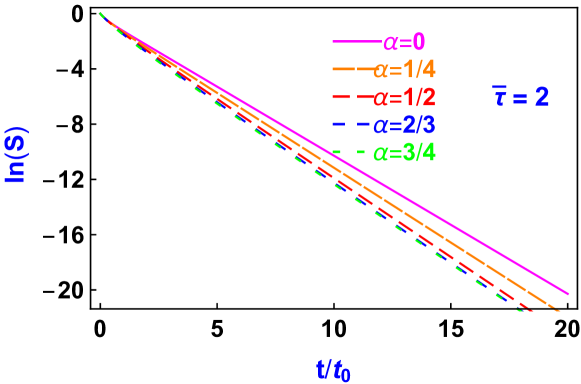
Figure 2: Plots of survival probability as a function of time $\bar{t}=t/t_{0}$ for different values of $\alpha$. $\bar{\tau}=\tau/t_{0}$ is taken to be $2$. The plots show that the decay is exponential for long times. Slopes obtained by fitting the data are given in Table 1.

$\hskip 8.5359pt\alpha\hskip 8.5359pt$	$\bar{k}_{eff}$ (fitted)	$\bar{k}_{eff}$ (from Eq. (29))
$0$	$0.9997$	$0.9999$
$\frac{1}{4}$	$1.0821$	$1.0824$
$\frac{1}{2}$	$1.1404$	$1.1398$
$\frac{2}{3}$	$1.1544$	$1.1398$
$\frac{3}{4}$	$1.1491$	$1.0968$

Table 1: Values of $k_{eff}$ for different values of $\alpha$. All the results are for $\bar{\tau}=2$.

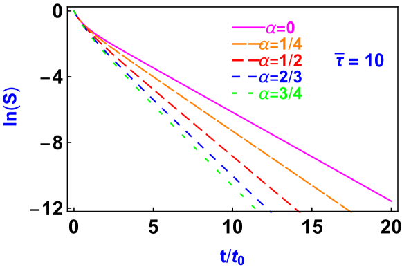
Figure 3: Plots of survival probability as a function of time $\bar{t}=t/t_{0}$ for different values of $\alpha$. $\bar{\tau}=\tau/t_{0}$ is taken to be $10$. The plots show that the decay is exponential for long times.

$\hskip 8.5359pt\alpha$	$\bar{k}_{eff}$ (fitted)	$\bar{k}_{eff}$ (from Eq. (29))
$0$	$0.5402$	$0.5403$
$\frac{1}{4}$	$0.6586$	$0.6575$
$\frac{1}{2}$	$0.8052$	$0.8000$
$\frac{2}{3}$	$0.9127$	$0.8910$
$\frac{3}{4}$	$0.9634$	$0.9038$

Table 2: Values of $\bar{k}_{eff}$ for different values of $\alpha$. All the results are for $\bar{\tau}=10$. It is to be noted that the agreement is good for smaller values of $\alpha$, but for $\alpha=3/4$, the agreement is not so good.

Figure 4: Plot of $\gamma$ and $\nu$ against $\alpha$.

It is clear that the long term decay is exponential, being of the form $e^{-k_{eff}t}$. From Eq. (27), an approximation to $k_{eff}$ is

$$k_{eff}=\frac{1}{\pi\tau}\int_{0}^{\infty}d\omega\ln\left(1+4k\tau\frac{k_{B}T}{m\omega_{0}^{2}}\;\frac{\cos\left(\frac{\pi\alpha}{2}\right)\omega^{-\alpha}}{(1+\omega^{2-2\alpha}+2\sin\left(\frac{\pi\alpha}{2}\right)\omega^{1-\alpha})}\right),$$ (28)

which in terms of the dimension-less quantities $\bar{t}$, $\bar{\tau}$ and $\bar{k}_{eff}=k_{eff}t_{0}$ may be written as

$$\bar{k}_{eff}=\frac{1}{\pi\bar{\tau}}\int_{0}^{\infty}d\omega\ln\left(1+4\bar{\tau}\;\frac{\cos\left(\frac{\pi\alpha}{2}\right)\omega^{-\alpha}}{(1+\omega^{2-2\alpha}+2\sin\left(\frac{\pi\alpha}{2}\right)\omega^{1-\alpha})}\right).$$ (29)

For $\alpha=0$, the integral can be evaluated exactly, to get the result

$$\bar{k}_{eff}=\frac{1}{\bar{\tau}}\left(\sqrt{1+4\bar{\tau}}-1\right),$$ (30)

which is the same as that obtained by Zwanzig (Zwanzig, 1992) (Note that while Zwanzig considers one dimensional version of the problem, while our analysis is for a two dimensional opening, and hence Zwanzig’s rate is only half of ours). On taking $\tau\propto\zeta\propto\eta$, for large values of $\frac{k_{B}T}{m\omega_{0}^{2}}$ (i.e., $\bar{\tau}\gg 1$), we find $k_{eff}\propto\eta^{-1/2},$ which is the result of Zwanzig. We now consider the situation where the radius of the opening undergoes subdiffusion. For $\alpha>0,$ we have not been able to evaluate $k_{eff}$ analytically. Hence we calculate the integral in Eq. (28) numerically, and find its dependence on $\zeta.$ We took $\bar{\tau}$ to be large and to vary from $1000$ to $10,000$. The value of $\overline{k}_{eff}$ was calculated for each $\bar{\tau}$, using Eq. (28) and MATHEMATICA. For each value of $\alpha$, plots of $\ln\bar{k}_{eff}$ against $\ln\bar{\tau}$ were then made, and were found to be linear with negative slope. This implies $\bar{k}_{eff}\propto(\bar{\tau})^{-\gamma}.$ As $\bar{\tau}\propto\zeta^{1/(1-a)}$ (see Eq. (10)), we get $\bar{\tau}\propto\eta^{-\nu}$, with $\nu=\gamma/(1-\alpha)$. The results for $\gamma$ and $\nu$ are plotted in Fig. LABEL:4-nuvsalp, for various values of $\alpha$. It is clear that the values range from $0.5$ to greater than unity (it is greater than unity for values of $\alpha$ very close to $1$). Remembering that $\zeta$ is proportional to the viscosity $\eta$, this is in better agreement with the experiments, than the simple diffusive model to Zwanzig (Zwanzig, 1992), or the stretched exponential model of Wang and Wolynes (Wang and Wolynes, 1993).

IV Summary and Conclusions

We have found exact solution to the problem of the survival probability of a Brownian oscillator that undergoes sub-diffusion, moving in presence of a quadratic sink. This is a problem of great interest in different areas of chemical physics Zwanzig (1992); Bian et al. (2015); Wang and Wolynes (1993) and for which only approximate solutions were known Bian et al. (2015). Our solution was used to analyse the problem of ligand passage through a fluctuating bottle neck. It was found that the model predicts an effective rate constant proportional to $\eta^{-\nu}$, $\eta$ being the viscosity of the medium, with a $\nu\geq 1/2$. This is in better agreement with experiments ($\nu$ in the range $0.4$ to $0.8$) than the previous models, which predict $\nu\leq 1/2$ Zwanzig (1992); Wang and Wolynes (1993). Hence sub-diffusion Kou and Xie (2004); Zheng et al. (2015) of the opening can explain the experimental observations Beece et al. (1980); Zwanzig (1992) on the viscosity dependence of ligand binding to a protein.

As already pointed out, there is experimental evidence for sub-diffusive motion (Yang et al., 2003; Kou and Xie, 2004; Min et al., 2005; Min and Xie, 2006) of the distance between two parts of a protein that are not directly bonded. There is also theoretical evidence for the same, for a simple polymer model (Dua and Adhikari, 2011). It would be nice to have more experimental and theoretical evidence in this direction. An attractive possibility would be to analyse the dynamics of the area of a gate using molecular dynamics simulations, as in (Nury et al., 2010).

V Acknowledgements

I thank Prof. Samuel C Kou (Harvard University) for making me aware of, and sending me a copy of the reference (Qian and Kou, 2014). This work was supported by the Department of Science and Technology, Government of India, through the J.C. Bose Fellowship.

References

- Zwanzig (1992) R. Zwanzig, Journal of Chemical Physics 97, 3587 (1992).
- Glarum (1960) S. H. Glarum, Journal of Chemical Physics 33, 1371 (1960).
- Hunt and Powles (1966) B. I. Hunt and J. Powles, Proceedings of Physical Society 88, 513 (1966).
- Bordewijk (1975) P. Bordewijk, Chemical Physics Letters 32, 592 (1975).
- Frobose and Jackle (1986) K. Frobose and J. Jackle, Journal of Statistical Physics 42, 551 (1986).
- Klafter and Blumen (1985) J. Klafter and A. Blumen, Chemical Physics Letters 293, 377 (1985).
- Beece et al. (1980) D. Beece, L.Eisenstein, and H. Frauenfelder, Biochemistry 19, 5147 (1980).
- Wang and Wolynes (1993) J. Wang and P. Wolynes, Chemical Physics Letters 212, 427 (1993).
- Eizenberg and Klafter (1996) N. Eizenberg and J. Klafter, Journal of Chemical Physics 104, 6796 (1996).
- Berezhkovskii et al. (1998) A. M. Berezhkovskii, Y. A. D’yakov, J. Klafter, and V. Y. Zitserman, Chemical Physics Letters 287, 442 (1998).
- Seki and Tachiya (2000) K. Seki and M. Tachiya, Journal of Chemical Physics 113, 3441 (2000).
- Berezhkovskii and Shvartsman (2016) A. M. Berezhkovskii and S. Y. Shvartsman, Journal of Chemical Physics 144, 204101 (2016).
- Bicout and Szabo (1998) D. J. Bicout and A. Szabo, Journal of Chemical Physics 108, 5491 (1998).
- Yang et al. (2003) H. Yang, G. Luo, P. Karnchanaphanurach, and X. S. Xie, Science 302, 262 (2003).
- Kou and Xie (2004) S. C. Kou and X. S. Xie, Physical Review Letters 93, 1 (2004).
- Min et al. (2005) W. Min, G. Luo, B. J. Cherayil, S. C. Kou, and X. S. Xie, Physical Review Letters 94, 1 (2005).
- Min and Xie (2006) W. Min and X. S. Xie, Physical Review E 73, 010902 (2006).
- Wang et al. (2009) B. Wang, S. M. Anthony, S. C. Bae, and S. Granick, Proceedings of the National Academy of Sciences of the United States of America 106, 15160 (2009), ISSN 1091-6490.
- Chubynsky and Slater (2014) M. V. Chubynsky and G. W. Slater, Physical Review Letters 113, 098302 (2014), ISSN 0031-9007, URL http://link.aps.org/doi/10.1103/PhysRevLett.113.098302.
- Metzler (2017) R. Metzler, Biophysical Journal 0112, 413 (2017).
- Jain and Sebastian (2016a) R. Jain and K. Sebastian, Journal of Physical Chemistry B 120 (2016a).
- Jain and Sebastian (2016b) R. Jain and K. L. Sebastian, The Journal of Physical Chemistry B 120, 9215 (2016b).
- Jain and Sebastian (2017a) R. Jain and K. Sebastian, Physical Review E 95 (2017a).
- Jain and Sebastian (2017b) R. Jain and K. Sebastian, Journal of Chemical Sciences 129, 929 (2017b).
- Jain and Sebastian (2017c) R. Jain and K. Sebastian, Journal of Chemical Physics 146, 214102 (2017c).
- Bian et al. (2015) Y. Bian, Z. Wang, A. Chen, and N. Zhao, Journal of Chemical Physics 143 (2015).
- Chatterjee and Cherayil (2010) D. Chatterjee and B. J. Cherayil, J. Chem. Phys. 132, 25103 (2010).
- Wang and Wolynes (1994) J. Wang and P. Wolynes, Chemical Physics 180, 141 (1994).
- Dua and Adhikari (2011) A. Dua and R. Adhikari, Journal of Statistical Mechanics: Theory and Experiment 2011, P04017 (2011).
- Kou (2008) S. C. Kou, The Annals of Applied Statistics 2, 501 (2008).
- Qian and Kou (2014) H. Qian and S. C. Kou, Annual Review of Statistics and its Application 1, 465 (2014).
- Chaichian and Demichev (2001) M. Chaichian and A. Demichev, Path Integrals in Physics. Volume I, Stochastic Processes and Quantum Mechanics (Institute of Physics Publishing, 2001).
- Zinn-Justin (2005) J. Zinn-Justin, Path Integrals in Quantum Mechanics (Oxford University Press, Oxford, 2005).
- Zheng et al. (2015) W. Zheng, D. De Sancho, T. Hoppe, and R. B. Best, Journal of the American Chemical Society 137, 3283 (2015).
- Nury et al. (2010) H. Nury, F. Poitevin, C. Van Renterghem, J.-P. Changeux, P.-J. Corringer, M. Delarue, and M. Baaden, Proceedings of the National Academy of Sciences 107, 6275 (2010), ISSN 0027-8424.