Channel Estimation for WiFi Prototype Systems with Super-Resolution Image Recovery

Abstract

Channel estimation is crucial for modern WiFi system and becomes more and more challenging with the growth of user throughput in multiple input multiple output configuration. Plenty of literature spends great efforts in improving the estimation accuracy, while the interpolation schemes are overlooked. To deal with this challenge, we exploit the super-resolution image recovery scheme to model the non-linear interpolation mechanisms without pre-assumed channel characteristics in this paper. To make it more practical, we offline generate numerical channel coefficients according to the statistical channel models to train the neural networks, and directly apply them in some practical WiFi prototype systems. As shown in this paper, the proposed super-resolution based channel estimation scheme can outperform the conventional approaches in both LOS and NLOS scenarios, which we believe can significantly change the current channel estimation method in the near future.

I Introduction

Channel estimation is often regarded as a critical component for modern wireless systems [24]. By inserting pre-known pilot sequences along with the transmit data, receivers shall be able to estimate the real-time wireless environment accordingly and perform coherent detection thereafter. Since the pilots consume air interface resources without useful information delivery, the existing literature spends tremendous efforts [18] in improving channel estimation accuracy, especially for multiple input multiple output (MIMO) orthogonal frequency division multiplexing (OFDM) configurations, which is commonly adopted in current cellular or wireless local area networks (WLAN) systems.

Along with the explosive growth of user throughput requirement for future wireless systems, the dimensions of available channels become huge when massive antennas and frequency bands have been aggregated and the accurate channel estimation under high dimensional signal spaces becomes much more challenging [25]. Several interesting schemes have been proposed to address this issue. For example, by recognizing the sparsity of MIMO channel characteristics, [19] proposes a distributed compressive sensing scheme with a few pilots for channel state recovery in MIMO systems. While for the case of broadband communication, [22] develops the matching pursuit based channel estimator which is an efficient method for the problem of multipath propagation. In [8], the authors utilize the non-orthogonal concept to aggregate multiple pilots together and improve the potential resolution of high dimension channel spaces. Nevertheless, the above schemes rely on abstracted channel models with certain characteristics, such as channel sparsity, and the application to practical systems is still challenging， especially when the hardware imperfectness has been considered [5].

In addition to the model based channel estimation schemes, the model-free channel estimation approaches, together with recent development of deep learning technologies, have been considered for practical wireless communication systems. For example, [29] utilizes deep neural networks (DNN) to combine the channel estimation and signal detection procedures in the conventional OFDM systems. In [9], a learned denoising-based approximate message passing (LDAMP) neural network has been proposed to reduce the noise effect in the iterative sparse channel estimation processes. The above methods provide insightful results on facilitating the deep learning technology for wireless application, which combines with several wireless domain knowledge, such as channel statistics or noise distributions. In this paper, however, we consider the domain knowledge from the image recovery area, where the deep learning technology has been successfully applied. To be more specific, super-resolution (SR), a deep-learning based image reconstruction technique, is proposed to recover the channel state information (CSI) from the limited observations of pilot signals and the main contributions of this paper are summarized as follows.

• Channel State Recovery versus Interpolation The existing literature for channel estimation focuses on the channel state recovery, which obtains CSI knowledge from the received pilot signals [24], while the interpolation schemes to calculate CSI values at wireless data transmission areas receive limited research attention. This is partially because the non-linear interpolation relation is challenging to characterize and the real-time requirement of channel estimation prevents complicated interpolation algorithms. In this paper, we exploit the SR image recovery scheme to model the non-linear interpolation relations in the conventional channel estimation problems, which does not rely on any pre-assumed statistical channel knowledge.

• Numerical versus Practical In the practical wireless systems, the true CSI knowledge can be hardly obtained. To make the proposed SR based channel estimation approach feasible, we offline generate some numerical channel coefficients according to the statistical channel models to train the SR neural networks, and then apply them online to some practical WiFi prototype systems. As we will show later, the proposed SR based channel estimation scheme can outperform several baseline schemes, which can provide some design insights for future deep learning based wireless communication system.

The rest of the paper is organized as follows. In Section II, we introduce the widely used MIMO-OFDM system model and summarize the traditional channel estimation as well as interpolation schemes. A brief formulation using SR framework for channel estimation is proposed in Section III and the associated neural network is analyzed in Section IV. In Section V, we verify the estimation accuracy via practical measurements by comparing the proposed SR based channel estimation scheme with conventional baselines and final remarks are given in Section VI.

Notations: Boldface uppercase and lowercase denote matrices and vectors, respectively, and the matrix inverse and conjugate transpose operations are given by $(\cdot)^{-1}$ and $(\cdot)^{H}$. $\mathbb{E}\left[\cdot\right]$ defines the mathematical expectation, while the matrix Frobenius is given by $\|\mathrm{\cdot}\|_{F}$.

II System Model and Conventional Schemes

In this section, we introduce the mathematical model for general MIMO-OFDM systems and explain the conventional channel state recovery and interpolation mechanisms in details.

II-A System Model

Consider a typical MIMO-OFDM system, as is depicted in Fig. 1, with $N_{t}$ transmit and $N_{r}$ receive antennas in the wireless fading environment. The received symbols at the $i^{th}$ subcarrier, $\mathbf{y}_{i}(t)\in\mathbb{C}^{N_{r}\times 1}$, after the Fast Fourier Transform (FFT) processing, can be modeled through,

$$\mathbf{y}_{i}(t)=\mathbf{H}_{i}(t)\mathbf{x}_{i}(t)+\mathbf{n}_{i}(t),$$ (1)

where $\mathbf{H}_{i}(t)\in\mathbb{C}^{N_{r}\times N_{t}}$ denotes the MIMO fading coefficients, $\mathbf{x}_{i}(t)\in\mathbb{C}^{N_{t}\times 1}$ denotes the transmitted symbols, and $\mathbf{n}_{i}(t)\in\mathbb{C}^{N_{r}\times 1}$ denotes the additive white Gaussian noise (AWGN) with zero mean and unit variance. Based on the observed $\mathbf{y}_{i}(t)$ and the pre-known pilot sequences $\mathbf{x}_{i}(t)$, we can recover the channel coefficients $\mathbf{H}_{i}(t)$ accordingly.

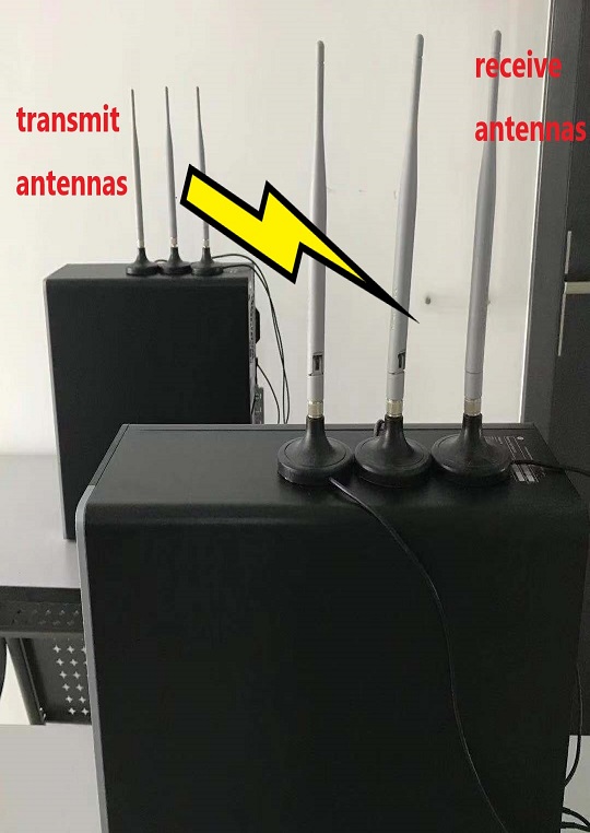
(a) Real Deployment

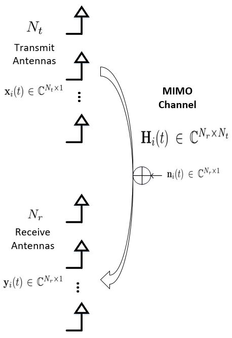
(b) System Model

Figure 1: An overview of WiFi prototype systems with $N_{r}\times N_{t}$ antenna configurations. Sub-figure (a) shows the real deployment of WiFi prototype systems and the abstracted model is shown in sub-figure (b). The MIMO channel conditions between transmit and receive antenna pairs for subcarrier $i$ are denoted as $\mathbf{H}_{i}(t)$.

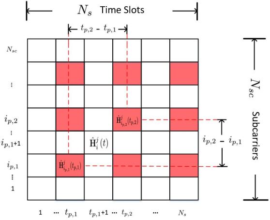
Figure 2: Illustration of interpolation mechanisms within one RB, containing $N_{sc}$ subcarriers in the frequency domain and $N_{s}$ slots in the time domain. Red grids represent the pilot locations, and the channel conditions at white grids are estimated through interpolation mechanisms defined in $\eqref{eqn:LI}$ and $\eqref{eqn:GI}$.

In the practical system, to minimize the channel estimation overhead, the entire process is performed on a resource block (RB) basis (usually in accordance with the coherence time and coherence bandwidth) with $N_{s}$ time slots and $N_{sc}$ subcarriers as shown in Fig. 2. Denote $\mathbf{H}_{i}^{j}(t)$ to be the MIMO fading coefficients for the $j^{th}$ RB, and by arranging them in order, we can obtain the entire channel condition, $\mathbf{H}^{j}$, as follows,

$$\mathbf{H}^{j} = \{\mathbf{H}_{i}^{j}(t)\},$$ (2)

$$= \left[\begin{matrix}\mathbf{H}_{1}^{j}(1)&\mathbf{H}_{1}^{j}(2)&\cdots&\mathbf{H}_{1}^{j}(N_{s})\\ \mathbf{H}_{2}^{j}(1)&\mathbf{H}_{2}^{j}(2)&\cdots&\mathbf{H}_{2}^{j}(N_{s})\\ \vdots&\vdots&\ddots&\vdots\\ \mathbf{H}_{N_{sc}}^{j}(1)&\mathbf{H}_{N_{sc}}^{j}(2)&\cdots&\mathbf{H}_{N_{sc}}^{j}(N_{s})\\ \end{matrix}\right].$$

In addition, to control the resource usage for channel estimation, only limited locations are selected for pilot allocation. Denote $\Omega_{p}$ to be the collections of pilot positions and the aggregated CSIs for pilots can be expressed through,

$$\mathbf{H}^{j}_{p}=\left\{\mathbf{H}_{i_{p}}^{j}(t_{p}),\forall(i_{p},t_{p})\in\Omega_{p}\right\},$$ (3)

where $i_{p}$ and $t_{p}$ denote the indexes of subcarrier and time slot within RB.

II-B Conventional Schemes

In the conventional channel estimation process, receivers perform channel state recovery to obtain an estimated channel conditions at the pilot positions, $\hat{\mathbf{H}}^{j}_{p}=\{\hat{\mathbf{H}}_{i_{p}}^{j}(t_{p}),\forall(i_{p},t_{p})\in\Omega_{p}\}$, and then apply interpolation mechanisms to get the entire channel coefficients, $\hat{\mathbf{H}}^{j}=\{\hat{\mathbf{H}}_{i}^{j}(t)\}$.

II-B1 Channel State Recovery

As mentioned before, the channel state recovery aims to obtain CSI knowledge at the pilot locations. For all the possible $(i_{p},t_{p})\in\Omega_{p}$, we can rewrite (1) as follows,

$$\mathbf{y}^{j}_{i_{p}}(t_{p})=\mathbf{H}^{j}_{i_{p}}(t_{p})\mathbf{x}_{i_{p}}(t_{p})+\mathbf{n}^{j}_{i_{p}}(t_{p}),$$ (4)

where we omit the superscript $j$ for $\mathbf{x}_{i_{p}}(t_{p})$ as the same pilot sequences are adopted for different RBs in practical systems. With the above relation, the classical least square (LS) and minimum mean square error (MMSE) [12] estimation can be described through,

$$\hat{\mathbf{H}}_{i_{p}}^{j,\textrm{LS}}(t_{p}) = \mathbf{y}^{j}_{i_{p}}(t_{p})\mathbf{x}_{i_{p}}^{H}(t_{p})\left(\mathbf{x}_{i_{p}}(t_{p})\mathbf{x}_{i_{p}}^{H}(t_{p})\right)^{-1},$$ (5)

$$\hat{\mathbf{H}}_{i_{p}}^{j,\textrm{MMSE}}(t_{p}) = \mathbf{R}_{\mathbf{H}}\left[\mathbf{R}_{\mathbf{H}}+\left(\mathbf{x}_{i_{p}}(t_{p})\mathbf{x}_{i_{p}}^{H}(t_{p})\right)^{-1}\right]^{-1}$$ (6)

$$\hat{\mathbf{H}}_{i_{p}}^{j,\textrm{LS}}(t_{p}),$$

where the unit variance assumption for the additive noise $\mathbf{n}^{j}_{i_{p}}(t_{p})$ is applied and $\mathbf{R}_{\mathbf{H}}$ is the channel correlation matrix at the receiver side with $\mathbf{R}_{\mathbf{H}}=\mathbb{E}\left[\mathbf{H}_{i_{p}}(t)\mathbf{H}_{i_{p}}^{H}(t)\right]$.

II-B2 Interpolation Mechanisms

With the estimated channel states at pilot positions, $\hat{\mathbf{H}}^{j}_{p}$, the interpolation mechanisms target to find the function $G(\cdot)$ that can minimize average mean square estimation error of $\hat{\mathbf{H}}^{j}$. Mathematically, the interpolation process can be modeled as,

$$\begin{aligned} G^{\star}(\cdot)=&\mathop{\arg\min}_{G(\cdot)}&\lim_{J\rightarrow\infty}\frac{1}{J}\sum_{j=1}^{J}\|\mathbf{H}^{j}-\hat{\mathbf{H}}^{j}\|_{F}^{2},\\ &\textrm{subject to}&\hat{\mathbf{H}}^{j}=G\left(\hat{\mathbf{H}}^{j}_{p}\right).\qquad\end{aligned}$$ (7)

In the practical deployment, since the real channel responses $\mathbf{H}^{j}$ is difficult to obtain, the above minimization is in general difficult to solve. Existing approaches rely on some heuristic interpolation schemes, such as linear interpolation (LI) and Gaussian interpolation (GI) [32]. Specifically, given two neighboring pilot locations $(i_{p,1},t_{p,1})$ and $(i_{p,2},t_{p,2})$, for any $t_{p,1}\leq t\leq t_{p,2}$ and $i_{p,1}\leq i\leq i_{p,2}$, we have the linear and Gaussian interpolated results $\hat{\mathbf{H}}_{i,LI}^{j}(t)$ and $\hat{\mathbf{H}}_{i,GI}^{j}(t)$ as follows,

$$\hat{\mathbf{H}}_{i,LI}^{j}(t)=G_{LI}\left(\hat{\mathbf{H}}^{j}_{p}\right)=\left(1-\alpha\right)\left(1-\beta\right)$$

$$\times\hat{\mathbf{H}}_{i_{p,1}}^{j}(t_{p,1})+\alpha\beta\hat{\mathbf{H}}_{i_{p,2}}^{j}(t_{p,2}),$$ (8)

$$\hat{\mathbf{H}}_{i,GI}^{j}(t)=G_{GI}\left(\hat{\mathbf{H}}^{j}_{p}\right)=\frac{1}{4}\left(\alpha^{2}-\alpha\right)\left(\beta^{2}-\beta\right)$$

$$\times\hat{\mathbf{H}}_{2i_{p,1}-i_{p,2}}^{j}(2t_{p,1}-t_{p,2})+\left(1-\alpha^{2}\right)\left(1-\beta^{2}\right)\hat{\mathbf{H}}_{i_{p}}^{j}(t_{p})$$

$$+\frac{1}{4}\left(\alpha^{2}+\alpha\right)\left(\beta^{2}+\beta\right)\hat{\mathbf{H}}_{2i_{p,1}+i_{p,2}}^{j}(2t_{p,1}+t_{p,2}),$$ (9)

where $\alpha=\frac{i-i_{p,1}}{i_{p,2}-i_{p,1}}$ and $\beta=\frac{t-t_{p,1}}{t_{p,2}-t_{p,1}}$ denote the interpolation coefficients.

Although the channel state recovery and interpolation provides a useful solution to the channel estimation for MIMO-OFDM systems, the achievable estimation accuracy is limited due to the following reasons. First of all, the time/frequency domain channel responses are never flat within each RB and the LI or GI can not well approximate the nonlinear variations in the practical scenarios. Second, the spatial correlations among different antennas are ignored in the current approach, which can be exploited via more complicated functions of $G(\cdot)$. Last but not least, the estimation performance can be further enhanced via a joint optimization for channel state recovery and interpolation.

III Super-Resolution Framework

In this section, we propose a novel interpolation scheme by applying the deep learning based SR image reconstruction technique, and elaborate the generation of data sets as well as the candidate neural networks.

III-A SR Formulation

Since the number of pilots, $N_{p}$, is always less than the number of resources, $N_{sc}\times N_{s}$, in each RB, the estimated channel conditions $\hat{\mathbf{H}}_{p}^{j}$ and $\hat{\mathbf{H}}^{j}$ can be regarded as low-resolution (LR) and high-resolution (HR) images with $N_{p}$ and $N_{sc}\times N_{s}$ pixels, respectively. Therefore, the function $G(\cdot)$ is a typical SR operation in the image processing area with the RGB color information determined by $N_{R}\times N_{T}$ complex numbers. With the above understanding, the SR framework as defined in [7] can be directly applied to approximate the optimal $G^{\star}(\cdot)$ as defined in (7), whose primary function is illustrated in Fig. 3.

As the objective function in (7) is the mean square errors (MSE) between the true channel condition $\mathbf{H}^{j}$ and the estimated channel condition $\hat{\mathbf{H}}^{j}$, we can construct the loss function in the deep learning based SR framework as,

$$\mathcal{L}\left(\hat{\mathbf{H}}^{j}\right)=\frac{1}{J}\sum_{j=1}^{J}\|\mathbf{H}^{j}-\hat{\mathbf{H}}^{j}\|_{F}^{2},$$ (10)

where the actual channel conditions $\mathbf{H}^{j}$ can be regarded as the ground truth HR image.

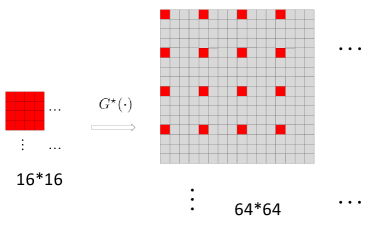
Figure 3: Illustration of optimal interpolation function $G^{\star}(\cdot)$, where the channel conditions estimated at the pilot locations ($16\times 16$ red grids) needs to be converted into $64\times 64$ grids via better interpolation mechanisms.

III-B Data Sets

Different from the traditional training data sets generation in the previous SR research, where a HR image is given in advance and the associated LR image is obtained through down-sampling, the true channel conditions $\mathbf{H}^{j}$ are difficult to collect in general. To overcome this obstacle, we generate $\mathbf{H}^{j}$ through a statistical channel model, e.g. COST 2100 as defined in [16], and simulate the pilot transmission process as defined in (4) via numerical examples. Based on the classical LS and MMSE estimation methods, e.g. (5) and (6), we generate LR images $\hat{\mathbf{H}}^{j,\textrm{LS}}_{p}=\left\{\hat{\mathbf{H}}^{j,\textrm{LS}}_{i_{p}}(t_{p})\right\}$ and $\hat{\mathbf{H}}^{j,\textrm{MMSE}}_{p}=\left\{\hat{\mathbf{H}}^{j,\textrm{MMSE}}_{i_{p}}(t_{p})\right\}$, respectively.

Through this approach, we can generate sufficient large size of data sets for training and evaluation, and to accommodate with the practical WiFi prototype system configuration, we choose $N_{r}=N_{t}=3$, $N_{sc}=64$, and $N_{s}=64$ in the SR neural network evaluation and optimization.

III-C Candidate Neural Networks

With the generated data sets and the clearly defined objective, we shall figure out the suitable neural network architecture for this type of application. Based on the existing literature, two types of neural networks show superior restoration performance over the traditional SR technology, which are summarized as follows.

• SR-CNN[7]: The LR image, $\hat{\mathbf{H}}_{p}^{j}$, is expanded to the HR image, $\hat{\mathbf{H}}_{LI}^{j}=\{\hat{\mathbf{H}}_{i,LI}^{j}(t)\}$ or $\hat{\mathbf{H}}_{GI}^{j}=\{\hat{\mathbf{H}}_{i,GI}^{j}(t)\}$, in the first stage, and then using neural networks to approximate the non-linear relation between $\hat{\mathbf{H}}_{LI}^{j}/\hat{\mathbf{H}}_{GI}^{j}$ and $\hat{\mathbf{H}}^{j}$.

• EDSR[15]: Apply a residual learning network [10] to progressively predict the SR images, $\hat{\mathbf{H}}^{j}$, from LR images, $\hat{\mathbf{H}}_{p}^{j}$.

Although the aforementioned deep learning based SR schemes achieves satisfied peak signal to noise ratio (PSNR) performance on the public data sets, such as BSD100 [2], the corresponding behaviors for approximating the optimal interpolation function $G^{\star}(\cdot)$ is still unknown.

IV SR Framework Analysis

In this section, we focus on analyzing the SR neural networks by comparing PSNR performance under the statistical COST 2100 channel models and exploits the possibility of applying SR based method for CSI estimation.

IV-A System Architecture

The architecture of SR-CNN and EDSR can be found in [7] and [15]. As is shown in Fig. 4,

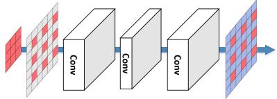
(a) SR-CNN

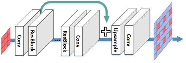
(b) EDSR

Figure 4: The network architecture of two typical SR neural networks, where sub-figure (a) and (b) demonstrates the abstracted network configuration of SR-CNN and EDSR, respectively. Different from the traditional linear interpolation or Gaussian interpolation, SR-CNN and EDSR approximate the non-linear interpolation via neural networks.

SR-CNN models the non-linear relationship between the LI$/$GI result and the real-time captured result, while EDSR applies massive residual network blocks to gradually generate the fine-grained result. Mathematically, the SR-CNN and EDSR based formulations are given as follows.

Problem 1 (SR-CNN Formulation)

In the SR-CNN formulation, the function $G^{\star}(\cdot)$ is approximated through $G^{\star}(\cdot)\approx G^{\star}_{CNN}(G_{LI/GI}(\cdot))$, with $G^{\star}_{CNN}(\cdot)$ given by

$$G^{\star}_{CNN}(\cdot) = \mathop{\arg\min}_{G_{CNN}(\cdot)}\lim_{J\rightarrow\infty}\frac{1}{J}\sum_{j=1}^{J}\|\mathbf{H}^{j}-\hat{\mathbf{H}}^{j}\|_{F},$$

$$\textrm{subject to}\ \hat{\mathbf{H}}^{j}=G_{CNN}\left(G_{LI/GI}\left(\hat{\mathbf{H}}^{j}_{p}\right)\right).$$

Problem 2 (EDSR Formulation)

In the EDSR formulation, we directly approximate $G^{\star}(\cdot)$ via progressively minimize the difference between the estimated results $\hat{\mathbf{H}}^{j}$ and the real channel state $\mathbf{H}^{j}$.

$$G^{\star}(\cdot) \approx G^{\star}_{EDSR}(\cdot)$$ (11)

$$= \mathop{\arg\min}_{G_{EDSR}(\cdot)}\lim_{J\rightarrow\infty}\frac{1}{J}\sum_{j=1}^{J}\|\mathbf{H}^{j}-\hat{\mathbf{H}}^{j}\|_{1},$$

$$\textrm{subject to}\ \ \hat{\mathbf{H}}^{j}=G_{EDSR}\left(\hat{\mathbf{H}}^{j}_{p}\right).$$

where $\|\cdot\|_{1}$ denotes the element-wise absolute value summation of the inner matrix.

From the above formulations, since SR-CNN focuses on the non-linear relationship between linear or Gaussian interpolated channel conditions and the real channel measurements, the optimization space for SR-CNN is in general limited. For EDSR, although the objective function is built on $l-1$ norm, the difference between $\|\mathbf{H}^{j}-\hat{\mathbf{H}}^{j}\|_{1}$ and the top of $\|\mathbf{H}^{j}-\hat{\mathbf{H}}^{j}\|_{F}$ is margined if $\|\mathbf{H}^{j}-\hat{\mathbf{H}}^{j}\|_{1}$ is sufficiently small. As a result, EDSR can provide better performance than SR-CNN approach under the same condition, which is verified in the coming subsection.

IV-B Network Training & Comparison

To generate sufficient data sets for neural network training, we consider the famous COST 2100 model to generate ${\mathbf{H}}^{j}$ as well as ${\mathbf{H}}_{p}^{j}$ as defined in Section II. To be more specific, the pilot positions are given by $\left\{\Omega_{p}:i_{p}\in\left\{1,5,9,\cdots,61\right\},\ t_{p}\in\left\{1,5,9,\cdots,61\right\}\right\}$ as shown in Fig. 3, and we generate $J=2000$ frames for the training and 200 frames for the validation test. The validation results are listed in Table I, comparing SR networks with conventional channel estimation methods mentioned in Section II, where the PSNR is selected as the performance metric. Based on Table I, EDSR takes the advantage of progressive learning for the entire function $G^{\star}(\cdot)$, which co-verifies the analysis in the previous subsection.

Table I: PSNR comparison of SR-CNN & EDSR based and conventional channel estimation schemes LS & MMSE

Interpolation Mechanisms	PSNR (LS/MMSE)
SR-CNN	25.7762$/$25.8396
EDSR	30.7883$/$31.0798
Linear Interpolation	21.0597$/$21.0671
Gaussian Interpolation	21.1140$/$21.1150

V Empirical Results

In this section, we deploy the SR based channel estimation scheme in the WiFi prototype systems using the trained SR neural network as illustrated in Section IV and provide some empirical results to show the effectiveness of the proposed channel estimation scheme by comparing with other traditional methods summerized in Section II. As shown in Fig. 1(a), two commercial desktops are communicating with each other through IEEE 802.11n WiFi protocols [1]. Since some of the subcarriers are muted as guard subcarriers in WiFi prototype systems, we slightly modify the input and output matrices, where $N_{sc}=N_{s}=56$ is selected and the number of pilots are scaled accordingly. The detailed parameters adopted in the evaluation are summarized in Table II.

Table II: Related Parameters Used in Evaluation

Scenario	COST 2100	WiFi Prototype
Frequency	5.3 GHz	5.32 GHz
Bandwidth	20 MHz	20 MHz
Antenna Configuration	3 $\times$ 3	3 $\times$ 3
Number of Packets	128000	60000

V-A LOS Scenario

In the first experiment, we compare the SR-CNN based channel estimation method with conventional schemes to show the effectiveness of the proposed SR based framework. LS and MMSE algorithms are adopted for channel state recovery at the pilot locations and we test two different pilot arrangements with $14\times 14$ and $28\times 28$ configurations. As is shown in Fig. 5, the SR-CNN based interpolation scheme outperforms the traditional LI or GI approach under both LS and MMSE channel state recovery methods, where the normalized MSE (NMSE) performance reduces from more than $-3$ dB to $-4$ dB. In addition, by comparing Real-SR-CNN and MMSE-SR-CNN curves, we can show that the SR networks trained from COST 2100 model is already sufficient for channel estimation in the practical system, and the NMSE loss is less than $0.2$ dB for $28\times 28$ case and $0.02$ dB for $14\times 14$ cases.

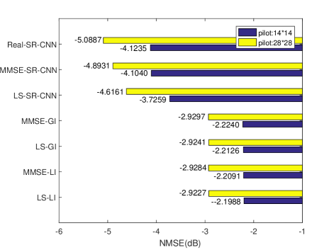
Figure 5: NMSE comparison of SR-CNN based and traditional channel estimation schemes in LOS environments. Two types of pilot arrangements are considered and the received SNR is fixed to 20 dB. As shown in this figure, the SR-CNN based channel estimation scheme outperforms the traditional LI and GI approaches for both two pilot arrangement cases.

V-B NLOS Scenario

In the second experiment, we extend the above experiments into NLOS scenario to show the robustness of the proposed algorithms in Fig. 6. Due to the potential scattering effects, the achievable NMSE will be degraded by $0.9$ dB for NLOS scenario. As the channel estimation in the NLOS environment is in general more difficult than LOS case as elaborated in [3], the proposed SR based channel estimation scheme achieves a reliable NMSE performance, which can be extended to NLOS application as well.

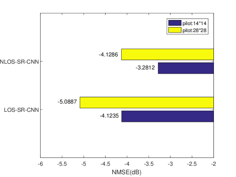
Figure 6: NMSE comparison of SR-CNN based and traditional channel estimation schemes in NLOS environments. Two types of pilot arrangements are considered and the received SNR is fixed to 20 dB. As shown in this figure, the SR based interpolation scheme achieves a reliable NMSE performance in NLOS conditions.

V-C Performance under EDSR

In the third experiment, we redo the above experiments by replacing the SR neural networks, e.g. from SR-CNN to EDSR. As EDSR provides better PSNR performance as shown in previous section, the better NMSE performance can be expected. As shown in Fig. 7, for both LOS and NLOS scenarios, EDSR based schemes achieve less than $-10$ dB NMSE for $14\times 14$ configuration and less than $-20$ dB NMSE for $28\times 28$ configuration. This is partially because the channel conditions are more close to sparse images and the gradually learning approach can adopt to the tiny variations.

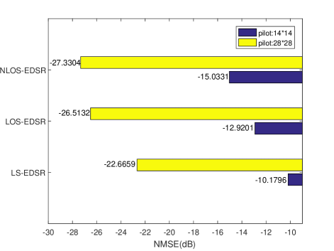
Figure 7: NMSE performance of EDSR networks under two different types of pilot arrangements in LOS and NLOS environments. The received SNR is fixed to 20 dB. As shown in this figure, the EDSR based channel estimation scheme achieves better NMSE performance in both LOS and NLOS conditions for two pilot arrangement cases.

VI Conclusion

In this paper, we propose a novel channel estimation method for WiFi prototype systems using SR based image recovery method. To make the proposed scheme more practical, we train the neural networks via numerical simulation results generated from COST 2100 model and directly apply it to the practical systems. Through the empirical examples, we show that the proposed SR based channel estimation methods provide significant performance gains in terms of NMSE over the traditional schemes in the prototype systems, which eventually benefits the channel estimation design for future wireless systems.

References

- [1] IEEE P802.11n-2009: Part 11: Wireless LAN Medium Access Control (MAC) and Physical Layer (PHY) Specifications Amendment 5: Enhancements for Higher Throughput, Oct. 2009.
- [2] Pablo Arbelaez, Michael Maire, Charless Fowlkes, and Jitendra Malik. Contour detection and hierarchical image segmentation. IEEE Trans. Pattern Anal. Mach. Intell., 33(5):898–916, Aug. 2011.
- [3] Francsco Benedetto, Gaetano Giunta, Alessandro Toscano, and Lucio Vegni. Dynamic LOS/NLOS statistical discrimination of wireless mobile channels. In IEEE Proc. VTC’07, pages 3071–3075, Apr. 2007.
- [4] Yajie Chai, Feng Hu, and Libiao Jin. A novel time interpolation channel estimation for IEEE802. 11ac system. In IEEE Proc. ICSESS’15, pages 722–725, Sep. 2015.
- [5] Xiang Cheng, Qi Yao, Miaowen Wen, Chengxiang Wang, Lingyang Song, and Bingli Jiao. Wideband channel modeling and intercarrier interference cancellation for vehicle-to-vehicle communication systems. IEEE J. Sel. Areas Commun., 31(9):434–448, Sep. 2013.
- [6] Carl De Boor. Bicubic spline interpolation. Wiley J. Math. Phys., 41(3):212–218, Apr. 1962.
- [7] Chao Dong, Change Loy Chen, Kaiming He, and Xiaoou Tang. Learning a deep convolutional network for image super-resolution. In Springer Proc. ECCV’14, volume 8692, pages 184–199, Sep. 2014.
- [8] Zhen Gao, Dai Linglong, Zhaocheng Wang, and Sheng Chen. Spatially common sparsity based adaptive channel estimation and feedback for FDD massive MIMO. IEEE Trans. Signal Process., 63(23):6169–6183, Jul. 2015.
- [9] Hengtao He, Chao Kai Wen, Shi Jin, and Geoffrey Ye Li. Deep learning-based channel estimation for beamspace mmwave massive MIMO systems. IEEE Wireless Commun. Lett., 7(5):852–855, Oct. 2018.
- [10] Kaiming He, Xiangyu Zhang, Shaoqing Ren, and Jian Sun. Deep residual learning for image recognition. In IEEE Proc. CVPR’16, pages 770–778, Jun. 2016.
- [11] Jakob Hoydis, Stephan Ten Brink, and Merouane Debbah. Massive MIMO in the UL/DL of cellular networks: How many antennas do we need? IEEE J. Sel. Areas Commun., 31(2):160–171, Feb. 2013.
- [12] Van De Beek Janjaap, Ove Edfors, Magnus Sandell, Sarah Kate Wilson, and Per Ola Borjesson. On channel estimation in OFDM systems. In IEEE Proc. VTC’95, volume 2, pages 815–819, Jul. 1995.
- [13] A Kutay, Haldun M Ozaktas, Orhan Ankan, and Levent Onural. Optimal filtering in fractional Fourier domains. IEEE Trans. Signal Process., 45(5):1129–1143, May. 1997.
- [14] Weisheng Lai, Jiabin Huang, Narendra Ahuja, and Minghsuan Yang. Deep Laplacian pyramid networks for fast and accurate super-resolution. In IEEE Proc. CVPR’17, pages 624–632, Jul. 2017.
- [15] Bee Lim, Sanghyun Son, Heewon Kim, Seungjun Nah, and Kyoung Mu Lee. Enhanced deep residual networks for single image super-resolution. In IEEE Proc. CVPRW’17, volume 1, pages 1132–1140, Jul. 2017.
- [16] L. Liu, C. Oestges, J. Poutanen, and K. Haneda. The COST 2100 MIMO channel model. IEEE Trans. Wireless Commun., 19(6):92–99, Dec. 2012.
- [17] Thomas L Marzetta. Noncooperative cellular wireless with unlimited numbers of base station antennas. IEEE Trans. Wireless Commun., 9(11):3590–3600, Oct. 2010.
- [18] Amine Mezghani and A Lee Swindlehurst. Blind estimation of sparse broadband massive MIMO channels with ideal and one-bit ADCs. IEEE Trans. Signal Process., 66(11):2972–2983, Mar. 2018.
- [19] Xiongbin Rao and Vincent KN Lau. Distributed compressive CSIT estimation and feedback for FDD multi-user massive MIMO systems. IEEE Trans. Signal Process., 62(12):3261–3271, May. 2014.
- [20] H R Sheikh, A C Bovik, and Veciana G De. An information fidelity criterion for image quality assessment using natural scene statistics. IEEE Trans. Image Process., 14(12):2117–2128, Nov. 2005.
- [21] Mehran Soltani, Ali Mirzaei, Vahid Pourahmadi, and Hamid Sheikhzadeh. Deep learning-based channel estimation. CoRR, abs/1810.05893, 2018.
- [22] Dongming Wang, Bing Han, Junhui Zhao, Xiqi Gao, and Xiaohu You. Channel estimation algorithms for broadband MIMO-OFDM sparse channel. In IEEE Proc. PIMRC’03, volume 2, pages 1929–1933, Sep. 2003.
- [23] Fanghua Weng, Changchuan Yin, and Tao Luo. Channel estimation for the downlink of 3GPP-LTE systems. In IEEE Proc. NIDC’10, pages 1042–1046, Sep. 2010.
- [24] Hongxiang Xie, Feifei Gao, and Shi Jin. An overview of low-rank channel estimation for massive MIMO systems. IEEE Access, 4(99):7313–7321, Nov. 2016.
- [25] Hongxiang Xie, Feifei Gao, Shi Jin, Jun Fang, and Yingchang Liang. Channel estimation for TDD/FDD massive MIMO systems with channel covariance computing. IEEE Trans. Wireless Commun., 17(6):4206–4218, Jun. 2018.
- [26] Hongxiang Xie, Feifei Gao, Shun Zhang, and Shi Jin. A unified transmission strategy for TDD/FDD massive MIMO systems with spatial basis expansion model. IEEE Trans. Veh. Technol., 66(4):3170–3184, Apr. 2017.
- [27] Yaxiong Xie, Zhenjiang Li, and Mo Li. Precise power delay profiling with commodity Wi-Fi. IEEE Trans. Mobile Comput., Jul. 2018.
- [28] Peng Xu, Jiangzhou Wang, Jinkuan Wang, and Feng Qi. Analysis and design of channel estimation in multicell multiuser MIMO OFDM systems. IEEE Trans. Veh. Technol., 64(2):610–620, Feb. 2015.
- [29] Hao Ye, Geoffrey Ye Li, and Biing Hwang Juang. Power of deep learning for channel estimation and signal detection in OFDM systems. IEEE Wireless Commun. Lett., 7(1):114–117, Feb. 2018.
- [30] Haifan Yin, David Gesbert, Miltiades Filippou, and Yingzhuang Liu. A coordinated approach to channel estimation in large-scale multiple-antenna systems. IEEE J. Sel. Areas Commun., 31(2):264–273, Feb. 2013.
- [31] Roman Zeyde, Michael Elad, and Matan Protter. On single image scale-up using sparse-representations. In Springer Proc. ICCS’12, volume 6920, pages 711–730, Jun. 2012.
- [32] Huaqing Zhang and Jianbo Liu. Two-dimension interpolation for OFDM channel estimation of DVB-T systems. In IEEE Proc. CMCE’10, volume 5, pages 253–256, Aug. 2010.
- [33] Dalin Zhu, Junil Choi, and Robert W Heath. Auxiliary beam pair enabled AoD and AoA estimation in closed-loop large-scale millimeter-wave MIMO systems. IEEE Trans. Wireless Commun., 16(7):4770–4785, Jul. 2017.