Gravitational-wave background from kink-kink collisions on infinite cosmic strings

Abstract

We calculate the power spectrum of the stochastic gravitational-wave (GW) background expected from kink-kink collisions on infinite cosmic strings. Intersections in the cosmic string network continuously generate kinks, which emit GW bursts by their propagation on curved strings as well as by their collisions. First, we show that the GW background from kink-kink collisions is much larger than the one from propagating kinks at high frequencies because of the higher event rate. We then propose a method to take into account the energy loss of the string network by GW emission as well as the decrease of the kink number due to the GW backreaction. We find that these effects reduce the amplitude of the GW background at high frequencies and produce a flat spectrum. Finally, we obtain a constraint on the string tension of $G\mu\lesssim 10^{-5}$ using the current upper bound on the GW background by Advanced LIGO, and $G\mu\lesssim 4\times 10^{-8}$ using pulsar timing arrays.

I I. Introduction

Cosmic strings are one-dimensional topological defects that may have been generated during a phase transition in the early Universe Kibble:1976sj . They are considered to form a network of infinite strings and loops, both of which have singular structures—called kinks and cusps—which emit strong gravitational-wave (GW) bursts Damour:2000wa ; Damour:2001bk . Overlapping bursts form a GW background, which can be tested by various GW experiments. In Ref. Kawasaki:2010yi and our previous work Matsui:2016xnp , the power spectrum of the GW background from kinks propagating on infinite strings was estimated using the number distribution of kinks derived in Ref. Copeland:2009dk . We have found that the GW background is generated over a wide range of frequencies, from the scale of the cosmic microwave background to direct-detection GW experiments.

In addition to GWs from kink propagation, kink-kink collisions are also expected to generate a GW background. Using the kink distribution derived in Copeland:2009dk , in this paper we calculate the power spectrum of the GW background originating from overlapping bursts from kink-kink collisions on infinite strings. We numerically calculate the kink number distribution as a function of time and sharpness, which gives the rate of kink-kink collisions, and estimate the amplitude of the GW spectrum by summing up the contribution from all of the redshifts. Since the result shows that kink-kink collisions generate a large GW background, we take into account two effects that could modify the estimate of the kink number distribution due to the large GW emission. The first effect is the energy loss of the string network through GW emission, which reduces the length of infinite strings. The second is the GW backreaction on kinks, which smooths out the kink sharpness. We include these factors in the calculation of the GW spectrum and, finally, compare it with the sensitivities of current and future GW experiments and discuss constraints on the cosmic string tension $G\mu$.

II II. Basic equations

The dynamics of cosmic strings is well described by the Nambu-Goto equations. By considering a spatially flat Friedmann-Lemaître-Robertson-Walker (FLRW) metric, ${\rm d}s^{2}=a^{2}(\tau)\left(-{\rm d}\tau^{2}+{\rm d}{\bf x}^{2}\right)$, choosing the coordinates on the worldsheet as $\tau$ (conformal time) and $\sigma$ (direction along a cosmic string), and using the gauge condition $\frac{\partial x^{\mu}}{\partial\tau}\frac{\partial x_{\mu}}{\partial\sigma}=0$, the Nambu-Goto action gives the evolution equation

$$\frac{\partial^{2}{\bf x}}{\partial\tau^{2}}+\frac{2}{a}\frac{{\rm d}a}{{\rm d}\tau}\frac{\partial{\bf x}}{\partial\tau}\Biggl{\{}1-\left(\frac{\partial{\bf x}}{\partial\tau}\right)^{2}\Biggr{\}}=\frac{1}{\epsilon}\frac{\partial}{\partial\sigma}\left(\frac{1}{\epsilon}\frac{\partial{\bf x}}{\partial\sigma}\right)\,,$$ (1)

where $\epsilon\equiv\sqrt{\frac{(\partial{\bf x}/\partial\sigma)^{2}}{1-(\partial{\bf x}/\partial\tau)^{2}}}$ is interpreted as energy per unit $\sigma$. In Minkowski spacetime, the solution is given by a linear superposition of left- and right-moving modes, ${\bf x}=({\bf a}+{\bf b})/2$. Here we introduce new variables ${\bf p}_{\pm}$, which represent left- and right-moving modes in the FLRW spacetime (corresponding to $\partial{\bf a}/\partial\sigma$ and $\partial{\bf b}/\partial\sigma$ in Minkowski spacetime), as

$${\bf p}_{\pm}\equiv\frac{\partial{\bf x}}{\partial\tau}\mp\frac{1}{\epsilon}\frac{\partial{\bf x}}{\partial\sigma}\,.$$ (2)

At a kink, the value of ${\bf p}_{\pm}$ changes discontinuously from ${\bf p}_{\pm,\,1}$ to ${\bf p}_{\pm,\,2}$. We define the sharpness of the kink as

$$\psi\equiv\frac{1}{2}(1-{\bf p}_{\pm,\,1}\cdot{\bf p}_{\pm,\,2})\,.$$ (3)

Cosmic strings obey a scaling law, in which the correlation length of cosmic strings evolves in proportion to the cosmic time $t$. The velocity-dependent one-scale (VOS) model Kibble:1984hp gives the evolution equations of the correlation length $L$ and the velocity $v$ as

$$\frac{{\rm d}L}{{\rm d}t} = HL(1+v^{2})+\frac{1}{2}cpv,$$ (4)

$$\frac{{\rm d}v}{{\rm d}t} = (1-v^{2})\left(\frac{k(v)}{L}-2Hv\right),$$ (5)

where $H$ is the Hubble parameter $H\equiv({\rm d}a/{\rm d}t)/a$ with $a(t)$ being the scale factor of the Universe and $k(v)$ is effective curvature $k(v)=\frac{2\sqrt{2}}{\pi}\frac{1-8v^{6}}{1+8v^{6}}$. The Hubble parameter is calculated as $H=H_{0}\sqrt{\Omega_{r}a^{-4}+\Omega_{m}a^{-3}+\Omega_{\Lambda}}$ with the Hubble constant $H_{0}=100h$km/s/Mpc. We use $\Omega_{r}h^{2}=4.31\times 10^{-5}$ and the cosmological parameters obtained from the Planck satellite: $h=0.692$, $\Omega_{\rm m}=0.308$, and $\Omega_{\Lambda}=0.692$ Ade:2015xua . The second term of Eq. (4) describes the loop production, and the value of the loop chopping efficiency $c$ is taken as $c\simeq 0.23$ Martins:2000cs . In this paper, we investigate the case of unit reconnection probability $p=1$, which is typical of field-theoretic strings. By simultaneously solving Eqs. (4) and (5), we obtain the solution of $L\propto t$ and we define the coefficient as $\gamma\equiv L/t$.

To calculate the GW background from kinks, we first estimate the distribution function of kinks $N(\psi,t)$, where $N(\psi,t){\rm d}\psi$ is the number of kinks between $\psi$ and $\psi+{\rm d}\psi$ within the arbitrary volume $V$. The evolution equation of $N(\psi,t)$ is written as Copeland:2009dk

$$\frac{\partial N}{\partial t}(\psi,\,t)=\frac{\bar{\Delta}V}{\gamma^{4}t^{4}}g(\psi)+\frac{2\zeta}{t}\frac{\partial}{\partial\psi}(\psi N(\psi,\,t))-\frac{\eta}{\gamma t}N(\psi,\,t).$$ (6)

The first term is the number of kinks produced by intersecting cosmic strings. The second term describes the blunting of kinks due to the expansion of the Universe. The third term is the number of kinks lost into loops. The parameters of each term in Eq.(6) are described as

$$\bar{\Delta} = \frac{2\pi}{35}\Bigl{\{}1+\frac{2}{3}(1-2v^{2})-\frac{1}{11}(1-2v^{2})^{2}\Bigr{\}},$$ (7)

$$\zeta = (1-2v^{2})\nu,$$ (8)

$$\eta = \frac{1}{2}cpv,$$ (9)

where $\nu$ is the parameter describing the time dependence of the scale factor $a\propto t^{\nu}$. By simultaneously solving Eqs. (4), (5), and (6), we obtain the distribution function of kinks. Figure 1 shows the number of kinks on infinite strings per unit length per logarithmic sharpness $\frac{\psi N(\psi,\,t)}{V(t)/(\gamma t)^{2}}$ as a function of $\psi$.

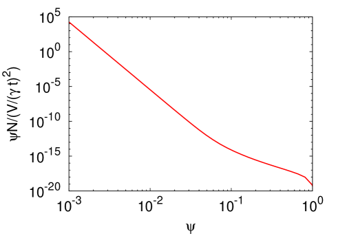
Figure 1: The distribution function of kinks on infinite strings. The number of kinks per unit length per logarithmic sharpness is shown as a function of sharpness.

From the figure, we see that kinks with small sharpness, which are produced in the radiation-dominated era, are more abundant than the ones with $\psi\sim 1$, which are produced recently. A more detailed explanation is given in Ref. Matsui:2016xnp .

III III. GW background

Next, we describe the method to calculate the GW background spectrum from kink-kink collisions. For comparison, we also describe the formalism for kinks propagating on infinite strings, which follows Ref. Matsui:2016xnp .

The Fourier strain amplitude of GWs from a propagating kink and a kink-kink collision are given, respectively, by Binetruy:2009vt

$$h_{\rm k}(\psi,f,z) = \frac{\psi^{1/2}G\mu\gamma t}{\{(1+z)f\gamma t\}^{2/3}}\frac{1}{r(z)}\Theta(1-\theta_{m}),$$ (10)

$$h_{\rm kk}(\psi,f,z) = \frac{\psi G\mu}{(1+z)f}\frac{1}{r(z)}\Theta(1-\theta_{m}),$$ (11)

where $f$ is the observed frequency so that $(1+z)f$ is the frequency at the emission, $\mu$ is the cosmic string tension, which becomes a dimensionless parameter $G\mu$ by multiplying it by the gravitational constant $G$, $r(z)=\int^{z}_{0}\frac{{\rm d}z}{H(z)}$ is the distance from the observer, and the first Heaviside step function $\Theta(1-\theta_{m})$ with $\theta_{m}\equiv\{(1+z)f\gamma t\}^{-1/3}$ plays the role to cutting off the long-wavelength mode beyond the string curvature $\gamma t$.

From Eq. (6), we obtain the number of kinks as a function of sharpness and $\psi\frac{N(\psi,\,t)}{V(t)/(\gamma t)^{2}}$ gives the number per unit length per logarithmic sharpness. The inverse of this gives the average interval of kinks with a given sharpness. Reference Kawasaki:2010yi investigated the GW background from kinks propagating on infinite strings and found that, for a given comoving GW frequency $f$, the dominant contribution on the GW background comes from kinks whose interval is the GW wavelength $\omega^{-1}$, where $\omega=2\pi f(1+z)$ is the physical GW angular frequency at the emission redshift $z$. Using the same discussion presented in the appendix of Ref. Kawasaki:2010yi , we can show that the same holds for the case of kink-kink collisions. For the sources at redshift $z$, the condition is given by

$$\left(\psi\frac{N(\psi,\,t)}{V(t)/(\gamma t)^{2}}\right)^{-1}\sim\omega^{-1}\,.$$ (12)

From now on, we denote the sharpness satisfying Eq. (12) as $\psi_{\rm m}$.

The power spectrum of the GW background is often characterized by $\Omega_{\rm gw}\equiv({\rm d}\rho_{\rm GW}/{\rm d}{\rm ln}f)/\rho_{c}$, where $\rho_{\rm GW}$ is the energy density of GWs and $\rho_{c}\equiv 3H^{2}/8\pi G$ is the critical density of the Universe. Using the effective GW burst rate $n(f,z)\equiv\frac{1}{f}\frac{{\rm d}\dot{N}}{{\rm d}\ln z}$, where $\dot{N}(f,z)$ is the event rate of GW bursts with frequency $f$ at redshift $z$, the power spectrum today is given by integrating contributions from all redshifts,

$$\Omega_{\rm GW}(t_{0},f)=\frac{2\pi^{2}f^{2}}{3H_{0}^{2}}\int\frac{{\rm d}z}{z}\Theta(n(\psi_{\rm m},f,z)-1)$$

$$\times n(\psi_{\rm m},f,z)h^{2}(\psi_{\rm m},f,z),$$ (13)

where we included the step function $\Theta(n(f,z)-1)$ to exclude rare bursts that do not overlap enough to form a GW background. Note that we only consider contributions from $\psi_{\rm m}$ according to the discussion around Eq. (12).

When one only considers contributions from kinks between $\ln\psi_{\rm m}$ and $\ln\psi_{\rm m}+{\rm d}\ln\psi_{\rm m}$, the event rate $n(\psi_{\rm m},f,z)$ can be estimated as

$$n(\psi_{\rm m},f,z)=\frac{1}{f}\times\left(\text{rate of GW bursts per kink})\right.$$

$$\times(\text{\# of kinks per unit volume }\frac{\psi_{\rm m}N(\psi_{\rm m},t)}{V})\times\frac{{\rm d}V(z)}{{\rm d}\,{\rm ln}z},$$

where $\frac{{\rm d}V}{{\rm d}z}=\frac{1}{z}\frac{{\rm d}V}{{\rm d}\ln z}=\frac{4\pi a^{3}r^{2}(z)}{H(z)}$ is the volume between $z$ and $z+{\rm d}z$. Using the beaming angle of GWs, $\frac{\theta_{m}}{2}$, and the typical curvature of the string $\gamma t$, the rate of GW bursts from a propagating kink is given by $\frac{\theta_{m}}{2(1+z)\gamma t}$, where $(1+z)$ is added to take into account the redshift of the time interval. For kink-kink collisions, the number of kinks per unit time crossing the path of any given kink is given by $\frac{\psi_{\rm m}N(\psi_{\rm m},t)}{V/(\gamma t)^{2}}$. By multiplying by $\frac{1}{2}$ to avoid double counting and taking into account the redshift, the rate of GW bursts per kink is given by $\frac{(\gamma t)^{2}}{2(1+z)}\frac{\psi_{\rm m}N(\psi_{\rm m},t)}{V}$. Note that a kink-kink collision emits GWs in all directions, and thus we do not multiply the rate by a beaming angle. In summary, the burst rates for propagating kinks and kink-kink collisions are written, respectively, as

$$n_{\rm k}(\psi_{\rm m},f,z) = \frac{1}{f}\frac{\theta_{m}}{2(1+z)\gamma t}\frac{\psi_{\rm m}N(\psi_{\rm m},t)}{V}\frac{{\rm d}V(z)}{{\rm d}\,{\rm ln}z},$$ (15)

$$n_{\rm kk}(\psi_{\rm m},f,z) = \frac{1}{f}\frac{(\gamma t)^{2}}{2(1+z)}\Bigl{\{}\frac{\psi_{\rm m}N(\psi_{\rm m},t)}{V}\Bigr{\}}^{2}\frac{{\rm d}V(z)}{{\rm d}\,{\rm ln}z}.$$

By substituting Eqs. (11) and (III) [Eqs. (10) and (15)] into Eq. (13), we obtain the GW background spectrum for kink-kink collisions (propagating kinks). Note that the value of $\psi_{\rm m}$ is time dependent and is estimated using Eq. (12) at every time step of the numerical calculation.

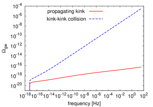
Figure 2: The power spectrum of the GW background from propagating kinks (red solid) and kink-kink collisions (blue dashed). For both lines, we assume $G\mu=10^{-11}$.

In Fig. 2 we compare the power spectrum of the GW background from propagating kinks and kink-kink collisions. Given the fact that $\psi\frac{N(\psi,\,t)}{V(t)/(\gamma t)^{2}}$ is a decreasing function of $\psi$, Eq. (12) indicates that the high-frequency GWs are produced by kinks with small sharpness, which have a high event rate. The large amplitude difference at high frequencies between the two cases arises because the event rate of kink-kink collisions increases in proportion to the square of the kink number, while the dependence is linear in the case of propagating kinks. One finds that the overproduction of GWs at high frequencies violates the constraints from big bang nucleosynthesis and the cosmic microwave background, $\Omega_{\rm GW}\lesssim 2\times 10^{-6}$ Cabass:2015jwe . However, this is not the final result and, in fact, it will be solved in the next section.

IV IV. Effects of GW emission

As shown in the previous section, the power spectrum increases dramatically towards high frequencies in the case of kink-kink collisions. One may be concerned that a large amount of GW emissions could change the number of infinite strings, since the energy of the string network is transferred to GWs. In addition, the backreaction of GW emission could smooth out the sharpness of kinks and reduce the power of GW emission. In this section, we take these two effects into account by modifying the VOS equation [Eq. (4)] and the evolution equation of the kink distribution [Eq. (6)], and recalculating the GW power spectrum.

Let us first consider the effect of GW radiation on the VOS equation Austin:1993rg ; Copeland:1999gn . The energy of GW emission from one kink-kink collision is estimated as $E_{\rm GW}\sim 2\pi^{3}\psi^{2}G\mu^{2}\omega^{-1}$ Binetruy:2009vt . Here, the factor $2\pi^{3}$ is added to make $E_{\rm GW}$ consistent with the expression for $\Omega_{\rm GW}$, that is, with the choice of the factor in front of $h_{\rm kk}$ in Eq. (11). Considering the energy conservation law for the string network density $\rho_{\infty}=\frac{\mu}{L^{2}}$ Martins:2000cs , the loss of energy density as GW radiation is given by

$$\frac{{\rm d}\rho_{\infty}}{{\rm d}t} = -\int_{0}^{1}{\rm d}\psi_{\rm m}\,E_{\rm GW}\times\text{(\# of GWs }$$

$$\hskip 70.0pt\text{ per unit volume, time, d$\psi_{m}$)},$$

$$= -\int_{0}^{1}{\rm d}\psi_{\rm m}\,2\pi^{3}\psi_{\rm m}^{2}G\mu^{2}\omega^{-1}~{}\frac{\psi_{\rm m}}{2}\left\{\frac{N(\psi_{\rm m},t)}{V/(\gamma t)^{2}}\right\}^{2}\frac{1}{(\gamma t)^{2}}.$$

Here, the integral in terms of d$\psi_{\rm m}$ corresponds to taking into account GWs of all frequencies. By rewriting $\rho_{\infty}$ in terms of $L$ and adding it to Eq. (4), we get

$$\frac{{\rm d}L}{{\rm d}t}=HL(1+v^{2})+\frac{1}{2}cpv+\frac{\pi^{3}G\mu}{2}\gamma t\int_{0}^{1}{\rm d}\psi_{\rm m}\,\frac{N(\psi_{\rm m},t)}{V/(\gamma t)^{2}}\psi_{\rm m}^{2},$$ (18)

where we have used Eq. (12) to replace $\omega$.

Next, we consider the GW backreaction on kinks and estimate the effect on the kink distribution. Before presenting the equations, let us compare the energy of one kink and the GW energy at one collision. When we treat a kink as a small perturbation $\delta{\bf p}_{\pm}$ Siemens:2001dx ; Copeland:2006if , the energy of the kink is estimated as $E_{\rm kink}=\mu(\delta{\bf p}_{\pm})^{2}\Delta\ell\sim\mu\psi\Delta\ell$ for a given length $\Delta\ell$, where we have used Eq. (3) in the second step. From Eq. (12), we expect that kinks contributing to the GW background are distributed with an average interval of $\omega^{-1}$, so we take $\Delta\ell\sim\omega^{-1}$. By taking the ratio $E_{\rm GW}/E_{\rm kink}=2\pi^{3}\psi G\mu$, we find that the fraction of energy going to GW emission is initially as small as $\sim G\mu$ for newly formed kinks $\psi\sim 1$, and the fraction gets even smaller when the kink sharpness is made smaller by the expansion of the Universe. Thus, when we consider the GW energy at one collision, the GW backreaction seems to be negligible.

However, the accumulation of a small GW backreaction through a huge number of collisions could change the kink distribution. This can be implemented as a modification of Eq. (6). By considering the energy fraction going to GWs, the backreaction term can be written as

$$(\text{\# of kinks lost by GW emission per V, time, d$\psi_{m}$})$$

$$\sim\frac{E_{\rm GW}\times(\text{\# of GWs per V, time, d$\psi_{m}$})}{E_{\rm kink}\times(\text{\# of kinks per V})}$$

$$\hskip 140.0pt\times(\text{\# of kinks per V})$$

$$\sim(2\pi^{3}\psi G\mu)\frac{\frac{1}{2}\psi\Bigl{\{}\frac{N(\psi)}{V/(\gamma t)^{2}}\Bigr{\}}^{2}\frac{V}{(\gamma t)^{2}}}{N(\psi,\,t)}N(\psi,\,t).$$ (19)

By adding this term, Eq. (6) becomes

$$\frac{\partial N}{\partial t}(\psi,\,t) = \frac{\bar{\Delta}V}{\gamma^{4}t^{4}}g(\psi)+\frac{2\zeta}{t}\frac{\partial}{\partial\psi}(\psi N(\psi,\,t))-\frac{\eta}{\gamma t}N(\psi,\,t)$$ (20)

$$\hskip 50.0pt-\frac{\pi^{3}G\mu\psi^{2}(\gamma t)^{2}}{V}N^{2}(\psi,\,t).$$

In Figs. 3 and 4, we show the time evolution of $\gamma$ and the kink distribution, respectively, calculated by simultaneously solving the VOS equations with GW radiation [Eqs. (18) and (5)] and the equation for the kink distribution with GW backreaction [Eq. (20)]. From Fig. 3, we see that the correlation length does not change at first, but starts to increase when the GW radiation term becomes non-negligible compared to the Hubble term.

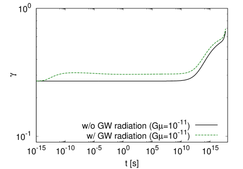
Figure 3: The time evolution of $\gamma$ calculated using Eqs. (18) and (20) for $10^{-11}$. For comparison, we also show the line calculated without the GW radiation term.

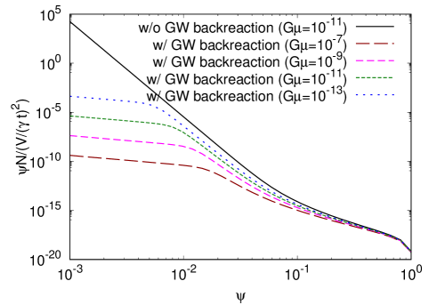
Figure 4: The distribution function of kinks calculated using Eqs. (18) and (20). The number of kinks per unit length per logarithmic sharpness is shown as a function of sharpness. Each line represents a different tension, from $G\mu=10^{-7}$ to $10^{-13}$. For comparison, we also show the line calculated using Eqs. (4) and (6).

In Fig. 4, we find that the number of kinks with small sharpness is suppressed, since the backreaction term in Eq. (20) affects the distribution when $N$ is large as it has a $\propto N^{2}$ dependence. We also see that the effect extends to larger sharpness when $G\mu$ is larger. The slope of the distribution function becomes gentler for large $G\mu$ because the value of $\gamma$ is larger due to the modification in Eq. (18).

Finally, in Fig. 5, we plot the power spectra of the GW background from kink-kink collisions for different $G\mu$. We see that high-frequency GWs are suppressed when we use the kink distribution with the GW modification. This is mainly because the number of small kinks is suppressed by the GW backreaction term in Eq. (20). We find that the suppression takes place at late times and it occurs earlier for smaller sharpness, which corresponds to high-frequency GWs. As a result, GWs of the high-frequency plateau are dominantly produced in kink-kink collisions in the radiation-dominated era, while ones in the small bump are produced in the matter-dominated era and ones in the low-frequency slope are generated today without being affected by the suppression. In the figure, we compare the spectra with the sensitivity curves of the future GW experiments SKA, LISA, DECIGO, and Advanced LIGO.

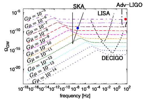
Figure 5: The power spectra of the GW background from kink-kink collisions for different string tensions, from $G\mu=10^{-5}$ to$10^{-14}$. We also show the sensitivities of the future observational instruments SKA, LISA, DECIGO, and Advanced LIGO. The red and blue circles represent the current upper limit on the GW amplitude by Advanced LIGO and NANOGrav.

We also plot the current upper limit on the GW background amplitude from the first observing run of Advanced LIGO, $\Omega_{\rm GW}<1.7\times 10^{-7}$ at 20-86 Hz TheLIGOScientific:2016dpb ; Abbott:2017mem , and the 11-year data set of NANOGrav, $\Omega_{\rm GW}h^{2}<3.4\times 10^{-10}$ at $3.2\times 10^{-8}$ Hz Arzoumanian:2018saf . We find that the current Advanced LIGO upper limit gives a constraint on the string tension of $G\mu\lesssim 10^{-5}$, and the NANOGrav constraint gives $G\mu\lesssim 4\times 10^{-8}$. In the future, Advanced LIGO operating at its full design sensitivity could provide $G\mu\lesssim 10^{-7}$, and pulsar timing with SKA could reach $G\mu\sim 10^{-11}$. With satellite experiments, we may be able to reach $G\mu\sim 10^{-11}$ using LISA and $G\mu\sim 10^{-13}$ using DECIGO.

V V. Discussion

Let us first discuss the spectral dependence of the GW background spectrum. When the GW backreaction is absent, one can find from Fig. 2 that the GW spectrum from kink-kink collisions scales as $\Omega_{\rm GW}\propto f^{0.77}$. This dependence is explained as follows. Substituting Eqs. (11) and (III) into Eq. (13), replacing the number of kinks with $f$ using Eq. (12), and leaving only the frequency and time dependence, we obtain

$$\Omega_{\rm GW}\propto\int{\rm d}({\rm ln}t)\,\frac{\psi_{\rm m}^{2}}{t(1+z)^{3}}f.$$ (21)

In our numerical calculation without the GW backreaction, we find that the contribution to the integration of $\Omega_{\rm GW}$ gets larger as the time increases for all of the frequencies. Thus, the shape of the GW spectrum is determined by the kink distribution today. From Fig. 1, we find $\psi\frac{N(\psi,\,t)}{V(t)/(\gamma t)^{2}}\propto\psi^{-8.8}$, and we get $\psi_{\rm m}\propto f^{-1/8.8}$ using Eq. (12). Substituting this into Eq. (21), we get $\Omega_{\rm GW}\propto f^{0.77}$. This frequency dependence continues up to the frequency where the oldest kinks (which have smallest sharpness) can generate GWs. Higher-frequency GWs are generated by kinks with smaller sharpness and the amplitude of the GW background starts to decrease at the frequency corresponding to the smallest kinks. This frequency is determined by the moment of time when cosmic strings were generated, which strongly depends on the generation model. Thus, in this paper we do not discuss the high-frequency behavior around the cutoff frequency.

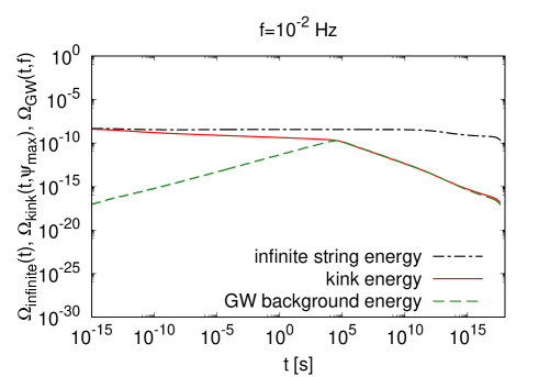
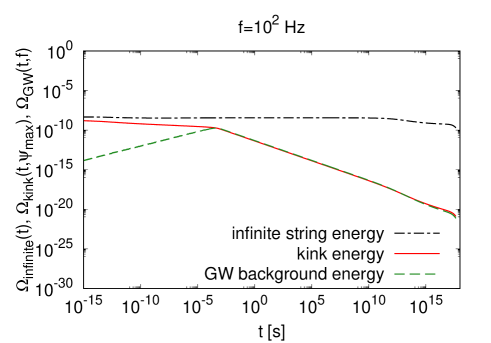
Figure 6: The time evolution of the infinite string energy density, the kink energy density, and the GW energy density produced at time $t$. The left panel is for kinks contributing to a GW frequency $f=10^{-2}$Hz and the right panel is for $10^{2}$Hz.

When we take the GW backreaction into account, we find that the number of kinks with small sharpness is suppressed, which reduces high-frequency GWs and creates a flat plateau in the spectrum. The reason for the flat spectrum is the following. The GW backreaction starts to affect kinks with small sharpness first, and the effect gradually extends to larger sharpness. Let us define the transition sharpness as $\psi_{\rm m,cut}(t)$, below which kinks are affected by the GW backreaction at time $t$. In the numerical calculation, we find that the contribution to the integration of $\Omega_{\rm GW}$ peaks when the backreaction starts to take affect, namely when $\psi_{\rm m}(t)=\psi_{\rm m,cut}(t)$. So let us evaluate Eq. (21) at the time $t_{c}$, which satisfies $\psi_{\rm m}(t_{c})=\psi_{\rm m,cut}(t_{c})$. Here we focus on the radiation-dominated era since $t_{c}$ is typically before radiation-matter equality for high-frequency GWs. Using $t\propto\frac{1}{(1+z)^{2}}$ and taking out only the contribution at $t_{c}$, Eq. (21) becomes

$$\Omega_{\rm GW}\propto\frac{\psi_{\rm m,cut}^{2}(t_{c})}{1+z_{c}}f.$$ (22)

Here, $z_{c}$ is the redshift at $t=t_{c}$, which depends on the frequency of interest $f$. Let us first see the time dependence of $\psi_{\rm m,cut}$. The GW backreaction starts to take effect when the fourth term becomes larger than the second and third terms in Eq. (20). Thus, we have

$$\left(\frac{\eta}{\gamma}-2\zeta\right)\frac{N}{t_{c}}=\pi^{3}G\mu\psi_{\rm m,cut}\Bigl{\{}\psi_{\rm m,cut}\frac{N}{V/(\gamma t_{c})^{2}}\Bigr{\}}N.$$ (23)

At early times, the backreaction term is negligible and the kink number evolves as $\psi\frac{N(\psi)}{V/(\gamma t)^{2}}\propto t^{-1}$, which is the analytic solution of Eq. (6) detailed in Ref. Copeland:2009dk . By substituting this into Eq.(23), we find that $\psi_{\rm m,cut}$ does not depend on time in the radiation-dominated era. The relation between $z_{c}$ and $f$ can be obtained using Eq. (12) as $2\pi f=\psi\frac{N(\psi,\,t)}{V(t)/(\gamma t)^{2}}\frac{1}{1+z}\propto(1+z)$. Applying this relation to Eq. (22), we get $\Omega_{\rm GW}\propto f^{0}$.

Next, let us see how the energy of GWs is balanced in the string network. We define the energy density parameter of kinks as

$$\Omega_{\rm kink}(t,\psi_{\rm m}) = \frac{E_{\rm kink}\times(\text{\# of kinks per unit volume})}{\rho_{c}}$$ (24)

$$\sim \frac{\mu\psi_{\rm m}\omega^{-1}\cdot\psi_{\rm m}\frac{N}{V/(\gamma t)^{2}}/(\gamma t)^{2}}{3H^{2}/(8\pi G)}$$

$$\sim \frac{8\pi G\mu}{3\gamma^{2}t^{2}H^{2}}\psi_{\rm m}.$$ (25)

In the second step, we have used Eq. (12). Note that this can be written as $\Omega_{\rm kink}=\psi_{m}\Omega_{\rm infinite}$, where $\Omega_{\rm infinite}\equiv\rho_{\infty}/\rho_{c}$. This indicates that the kink energy is always smaller than the total energy density of infinite strings by the order of the sharpness $\psi_{\rm m}$. In Fig. 6 we plot the time evolution of the infinite string energy density, the kink energy density, and the GW energy density produced at time $t$ [the integrand of Eq. (13) before redshifting]. The two panels show the GW frequencies $f=10^{-2}$ and $10^{2}$Hz, which correspond to different values of $\psi_{\rm m}$. As one can see, the energy of GWs increases at the beginning, and when it becomes comparable to the kink energy both the kink and GW energies start to decrease and evolve together. This behavior is due to the fact that the GW energy is balanced by the kink energy thanks to the GW terms added to the VOS equation [Eq. (18)] and the evolution equation for kink number density [Eq. (20)]. In summary, we find that the kink and GW energies become of the same order when the GW terms are turned on, and they always stay below the total energy of the scaling string network by the order of $\psi_{\rm m}$.

Finally, let us comment on previous works. The GW spectrum from small structures on infinite strings was calculated analytically in Refs. Sakellariadou:1990ne ; Hindmarsh:1990xi and numerical simulations for GWs from infinite strings were performed in Ref. Figueroa:2012kw . They all predicted a smaller GW amplitude compared to our result. We believe that the reason is because those previous studies only considered kinks with large sharpness $\sim 1$ (for simplicity in the analytic study, and because of the resolution in the simulation study), while our method based on solving the evolution equation of kink distribution (established in Ref. Copeland:2009dk ) enables us to take into account kinks with much smaller sharpness. In fact, we have seen that the enhancement of GWs occurs at high frequencies, which are mainly produced by kinks with small sharpness.

GWs from kink-kink collisions on loops were considered in Refs. Binetruy:2010cc ; Ringeval:2017eww ; Jenkins:2018nty . Although their estimate has some uncertainty since the number of kinks on one loop was taken as a free parameter in their calculation, it has been shown that a large GW background can be expected from kink-kink collisions on loops. We would like to mention that our estimate for the kink number distribution may help to determine the exact number of loops and may provide more concrete predictions.

VI VI. Conclusion

There have been many efforts to search for and constrain cosmic strings with cosmological observations. In this paper, we have shown a new way to test the existence of cosmic strings by considering kink-kink collisions on infinite strings. We have presented formulas to calculate the GW power spectrum from kink-kink collisions, which predict a much larger GW amplitude compared to the one from kink propagation. Furthermore, we have investigated the effect of GW radiation and backreaction on the scaling behavior and kink distribution, and found that these effects reduce the GW amplitude at high frequencies. Finally, by comparing with the upper bounds on the GW background amplitude from ongoing experiments, we obtained constraints on the string tension of $G\mu\lesssim 10^{-5}$ from Advanced LIGO, and $G\mu\lesssim 4\times 10^{-8}$ from NANOGrav. Although the current pulsar timing constraint from loops is stronger than these bounds, we would like to stress that our prediction based on infinite strings does not have any ambiguity on the initial loop size, which has been under debate and could weaken the pulsar timing constraint from loops. Therefore, our result can be used as an independent test of cosmic strings.

VII Acknowledgments

This work is partially supported by the Grant-in-Aid for Scientific Research from JSPS, Grant Number 17K14282, and by the Career Development Project for Researchers of Allied Universities (S. K.). We are deeply grateful to Danièle Steer for providing the initial idea and for useful comments which helped to enhance the quality of the work. S. K. would like to thank Jose J. Blanco-Pillado and Teruaki Suyama for helpful discussion.

References

- (1) T. W. B. Kibble, J. Phys. A 9, 1387 (1976).
- (2) T. Damour and A. Vilenkin, Phys. Rev. Lett. 85, 3761 (2000).
- (3) T. Damour and A. Vilenkin, Phys. Rev. D 64, 064008 (2001).
- (4) M. Kawasaki, K. Miyamoto, and K. Nakayama, Phys. Rev. D 81, 103523 (2010).
- (5) Y. Matsui, K. Horiguchi, D. Nitta, and S. Kuroyanagi, J. Cosmol. Astropart. Phys. 11 (2016) 005.
- (6) E. J. Copeland and T. W. B. Kibble, Phys. Rev. D 80, 123523 (2009).
- (7) T. W. B. Kibble, Nucl. Phys. B252, 227 (1985); B261, 750(E) (1985).
- (8) P. A. R. Ade et al. (Planck Collaboration), Astron. Astrophys. 594, A13 (2016).
- (9) C. J. A. P. Martins and E. P. S. Shellard, Phys. Rev. D 65, 043514 (2002).
- (10) P. Binetruy, A. Bohe, T. Hertog, and D. A. Steer, Phys. Rev. D 80, 123510 (2009).
- (11) G. Cabass, L. Pagano, L. Salvati, M. Gerbino, E. Giusarma, and A. Melchiorri, Phys. Rev. D 93, 063508 (2016).
- (12) D. Austin, E. J. Copeland, and T. W. B. Kibble, Phys. Rev. D 48, 5594 (1993).
- (13) E. J. Copeland, J. Magueijo, and D. A. Steer, Phys. Rev. D 61, 063505 (2000).
- (14) X. Siemens and K. D. Olum, Nucl. Phys. B611, 125 (2001); B645, 367(E) (2002).
- (15) E. J. Copeland, T. W. B. Kibble, and D. A. Steer, Phys. Rev. D 75, 065024 (2007).
- (16) B. P. Abbott et al. (LIGO Scientific and Virgo Collaborations), Phys. Rev. Lett. 118, 121101 (2017); 119, 029901(E) (2017).
- (17) B. P. Abbott et al. (LIGO Scientific and Virgo Collaborations), Phys. Rev. D 97, 102002 (2018).
- (18) Z. Arzoumanian et al. (NANOGRAV Collaboration), Astrophys. J. 859, 47 (2018).
- (19) M. Sakellariadou, Phys. Rev. D 42, 354 (1990); 43, 4150(E) (1991).
- (20) M. Hindmarsh, Phys. Lett. B 251, 28 (1990).
- (21) D. G. Figueroa, M. Hindmarsh, and J. Urrestilla, Phys. Rev. Lett. 110, 101302 (2013).
- (22) P. Binetruy, A. Bohe, T. Hertog, and D. A. Steer, Phys. Rev. D 82, 126007 (2010).
- (23) C. Ringeval and T. Suyama, J. Cosmol. Astropart. Phys. 12 (2017) 027.
- (24) A. Jenkins and M. Sakellariadou, Phys. Rev. D 98, 063509 (2018).