Neural Reverse Engineering of Stripped Binaries
using Augmented Control Flow Graphs

Abstract.

We address the problem of reverse engineering of stripped executables, which contain no debug information. This is a challenging problem because of the low amount of syntactic information available in stripped executables, and the diverse assembly code patterns arising from compiler optimizations.

We present a novel approach for predicting procedure names in stripped executables. Our approach combines static analysis with neural models. The main idea is to use static analysis to obtain augmented representations of call sites; encode the structure of these call sites using the control-flow graph (CFG) and finally, generate a target name while attending to these call sites. We use our representation to drive graph-based, LSTM-based and Transformer-based architectures.

Our evaluation shows that our models produce predictions that are difficult and time consuming for humans, while improving on existing methods by $28\%$ and by $100\%$ over state-of-the-art neural textual models that do not use any static analysis. Code and data for this evaluation are available at https://github.com/tech-srl/Nero.

1. Introduction

Reverse engineering (RE) of executables has a variety of applications such as improving and debugging legacy programs. Furthermore, it is crucial to analyzing malware. Unfortunately, it is a hard skill to learn, and it takes years to master. Even experienced professionals often have to invest long hours to obtain meaningful results. The main challenge is to understand how the different “working parts” inside the executable are meant to interact to carry out the objective of the executable. A human reverse-engineer has to guess, based on experience, the more interesting procedures to begin with, follow the flow in these procedures, use inter-procedural patterns and finally, piece all these together to develop a global understanding of the purpose and usage of the inspected executable.

Despite great progress on disassemblers [IDAPRO; RADAR], static analysis frameworks (Katz et al., 2018; Lee et al., 2011) and similarity detectors (David et al., 2017; Pewny et al., 2015), for the most part, the reverse engineering process remains manual.

Reviewing source code containing meaningful names for procedures can reduce human effort dramatically, since it saves the time and effort of looking at some procedure bodies (Alon et al., 2019c; Høst and Østvold, 2009; Fowler and Beck, 1999; Jacobson et al., 2011). Binary executables are usually stripped, i.e., the debug information containing procedure names is removed entirely.

As a result of executable stripping, a major part of a reverse engineer’s work is to manually label procedures after studying them. Votipka et al. (2020) detail this process in a user study of reverse engineers and depict their reliance on internal and external procedure names throughout their study.

In recent years, great strides have been made in the analysis of source code using learned models from automatic inference of variables and types (Raychev et al., 2015; Bielik et al., 2016; Alon et al., 2018; Bavishi et al., 2018; Allamanis et al., 2018) to bug detection (Pradel and Sen, 2018; Rice et al., 2017), code summarization (Allamanis et al., 2016; Alon et al., 2019c, a), code retrieval (Sachdev et al., 2018; Allamanis et al., 2015b) and even code generation (Murali et al., 2017; Brockschmidt et al., 2019; Lu et al., 2017; Alon et al., 2019b). However, all of these address high-level and syntactically-rich programming languages such as Java, C# and Python. None of them address the unique challenges present in executables.

Problem definition Given a nameless assembly procedure $\mathcal{X}$ residing in a stripped (containing no debug information) executable, our goal is to predict a likely and descriptive name $\mathcal{Y}=y_{1}...,y_{m}$, where $y_{1}...,y_{m}$ are the subtokens composing $\mathcal{Y}$. Thus, our goal is to model $P\left(\mathcal{Y}\mid\mathcal{X}\right)$. For example, for the name $\mathcal{Y}=$ create_server_socket, the subtokens $y_{1}...,y_{m}$ that we aim to predict are create, server and socket, respectively.

The problem of predicting a meaningful name for a given procedure can be viewed as a translation task – translating from assembly code to natural language. While this high-level view of the problem is shared with previous work (e.g., (Allamanis et al., 2016; Alon et al., 2019c, a)), the technical challenges are vastly different due to the different characteristic of binaries.

1: mov rsi, rdi
2: mov rdx, 16
3: mov rax, [rbp-58h]
4: mov rdi, rax
5: call connect
6: mov edx, eax
7: mov rax, [rbp-4h]
…
8: mov rax, [rbp-58h]
9: mov rdi, rax
10: mov r8, 4
11: mov rdx, 10
12: mov esi, 0
13: lea rcx, [rbp-88h]
14: call setsockopt
…
call printf
call close
3: call connect
call printf
2: call setsocketopt

(a)

(b)

(c)

(d) (a) The result of disassembing an optimized binary procedure taken from a stripped executable ; (b) The call instructions randomly placed in the procedure code by the compiler ; (c) the call instructions are placed in their correct call order as they appear in the CFG.

Challenge 1: Little syntactic information and token coreference Disassembling the code of a stripped procedure results in a sequence of instructions as the one in Fig. 1(a). These instructions are composed from a mnemonic (e.g., mov), followed by a mix of register names and alphanumeric constants. These instructions lack any information regarding the variable types or names that the programmer had defined in the high-level source code. Registers such as rsi and rax (lines 1, 7 in Fig. 1(a)) are referenced in different manners, e.g., rax or eax (lines 1, 12), and used interchangeably to store the values held by different variables. This means that the presence of a register name in an instruction carries little information. The same is true for constants: the number $4$ can be an offset to a stack variable (line 7), an Enum value used as an argument in a procedure call (line 10) or a jump table index.

Learning descriptive names for procedures from such a low-level stripped representation is a challenging task. A naïve approach, where the flat sequence of assembly instructions is fed into a sequence-to-sequence (seq2seq) architecture (Luong et al., 2015; Vaswani et al., 2017), yields imprecise results ($21.72$ F1 score), as we show in Section 6.

Challenge 2: Long procedure names Procedure names in compiled C code are often long, as they encode information that would be part of a typed function signature in a higher-level language (e.g., AccessCheckByTypeResultListAndAuditAlarmByHandleA in the Win32 API). Methods that attempt to directly predict a full label as a single word from a vocabulary will be inherently imprecise.

Our approach We present a novel representation for binary procedures specially crafted to allow a neural model to generate a descriptive name for a given stripped binary procedure. To construct this representation from a binary procedure we:

1. Build a control-flow graph (CFG) from the disassembled binary procedure input.

2. Reconstruct a call-site-like structure for each call instruction present in the disassembled code.

3. Use pointer-aware slicing to augment these call sites by finding concrete values or approximating abstracted values.

4. Transform the CFG into an augmented call sites graph.

This representation is geared towards addressing the challenge of analyzing non-informative and coreference riddled disassembled binary code (challenge 1).

In Section 5, we explain how this representation is combined with graph-based (Kipf and Welling, 2017), long short-term memory network (LSTM)-based (Sutskever et al., 2014; Luong et al., 2015) and Transformer-based (Vaswani et al., 2017) neural architectures. These architectures can decode long out-of-vocabulary (OOV) predictions to address the challenge of predicting long names for binary procedures (challenge 2).

This combination provides an interesting and powerful balance between the program-analysis effort required to obtain the representation from binary procedures, and the effectiveness of the learning model.

Existing techniques Debin (He et al., 2018) is a non-neural model for reasoning about binaries. This model suffers from inherent sparsity and can only predict full labels encountered during training.

DIRE (Lacomis et al., 2019) is a neural model for predicting variable names. DIRE uses the textual sequence (C code) created by an external black-box decompiler (Hex-Rays), accompanied by the abstract syntax tree (AST) to create a hybrid LSTM and graph neural network (GNN) based model.

In Section 6, we show that our approach outperforms DIRE and Debin with relative F1 score improvements of $28\%$ and $35\%$, respectively.

Main contributions The main contributions of this work are:

• A novel representation for binary procedures. This representation is based on augmented call sites in the CFG and is tailor-made for procedure name prediction.

• This representation can be used in a variety of neural architectures such as GNNs, LSTMs and Transformers (Section 4).

• Nero , A framework for binary name prediction. Nero is composed of: (i) a static binary analyzer for producing the augmented call sites representation from stripped binary procedures and (ii) three different neural networks for generating and evaluating name prediction .

• An extensive evaluation of Nero, comparing it with Debin, DIRE and state-of-the-art neural machine translation (NMT) models ((Luong et al., 2015; Vaswani et al., 2017)). Nero achieves an F1 score of $45.53$ in predicting procedure names within GNU packages, outperforming all other existing techniques.

• A thorough ablation study, showing the importance of the different components in our approach (Section 6.3).

2. Overview

In this section, we illustrate our approach informally and provide an example to further explain the challenges in binary procedure name prediction. This example is based on a procedure from our test set that we simplified for readability purposes. While this example is an Intel 64-bit Linux executable, the same process can be applied to other architectures and operating systems.

Using calls to imported procedures Given an unknown binary procedure $P$, which is stripped of debug symbols, our goal is to predict a meaningful and likely name that describes its purpose. After disassembling $P$’s code, the procedure is transformed into a sequence of assembly instructions. A snippet from this sequence is shown in Fig. 1(a).

We draw our initial intuition from the way a human reverse engineer skims this sequence of assembly instructions. The most informative pieces of information to understand what the code does are calls to procedures whose names are known because they can be statically resolved and can not be easily stripped. In our example, these are call connect (line $5$) and call setsockopt (line $14$) in Fig. 1(a). Resolving these names is possible because these called procedures reside in libraries that are dynamically linked to the executable, causing them to be imported (into the executable memory) as a part of the operating system (OS) loading process. We further discuss imported procedure name resolution in Section 4. Calls to such imported procedures are also called application program interface (API) calls, as they expose an interface to these libraries. We will refer to their names, e.g., connect and setsockopt, as API names.

In order to pass arguments when making these API calls, the calling convention used by the OS defines that these argument values are placed into specific registers before the call instruction. The process of assigning into these registers is shown in lines 1-4 and 8-13 of Fig. 1(a). Its important to note, while anti- reverse engineering (RE) tools may try and obfuscate API names, the values for the arguments passed when calling these external procedures must remain intact.

In Section 6 we discuss API name obfuscation and examine their effect on the performance of different approaches to procedure name prediction.

Putting calls in the right order After examining the API calls of the procedure, a human reverser will try to understand the order in which they are called at runtime. Figure 1(b) shows all the call instructions in $P$’s disassembled code, in the semi-random order in which they were generated by the compiler. This order does not reflect any logical or chronological order. For example, (i) the call to socket, which is part of the setup, is interleaved with printf used for error handling; and (ii) the calls in this sequence are randomly shuffled in the assembly, i.e., connect appears before setsocketopt .

To order the API calls correctly, we construct a CFG for $P$. A CFG is a directed graph representing the control flow of the procedure, as determined by jump instructions. Figure 1(c) shows a CFG created from the dissembled code in Fig. 1(a). For readability only, the API calls are presented in the CFG nodes (instead of the full instruction sequence). By observing the CFG, we learn all possible runtime paths, thus approximating all potential call sequences.

A human reverse-engineer can follow the jumps in the CFG and figure out the order in which these calls will be made: $\pi=$ socket$\rightarrow$setsockopt$\rightarrow$connect.

Reconstructing Call Sites Using Pointer-Aware Slicing After detecting call sites, we wish to augment them with additional information regarding the source of each argument. This is useful because the source of each argument can provide a hint for the possible values that this argument can store. Moreover, as discussed above, these are essential to allow name prediction in the face of API name obfuscation.

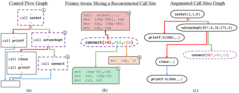
Figure 1. (a) The procedure’s CFG showing all call instructions, and focusing on the path leading to the call connect instruction is shown in dashed purple; (b) The reconstructed call site for connect connecting each argument register to its pointer aware slice ; (c) the augmented call sites graph containing the augmented call sites for all API calls, including connect.

Figure 1 depicts the process of creating our augmented call sites-based representation, focusing on the creation of the call site for the connect API call. Figure 1(a) depicts $P$’s CFG showing only call instructions.

We enrich the API call into a structure more similar to a call site in higher-level languages. To do so, we retrieve the number of arguments passed when calling an API by examining debug symbols for the library from which they were imported. Following the OS calling convention, we map each argument to the register used to pass it. By retrieving the three arguments for the connect API, we can reconstruct its call site: connect(rdi, rsi, rdx), as shown in Fig. 1(b). This reconstructed call site contains the API name (connect) and the registers that are used as arguments for this API call (rdi, rsi, rdx).

To obtain additional information from these call sites, we examine how the value of each argument was computed. To gather this information, we extract a static slice of each register at the call location in the procedure. A slice of a program (Weiser, 1984) at a specific location for a specific value is a subset of the instructions in the program that is necessary to create the value at this specific location.

\raisebox{0pt}{\footnotesize{1}}⃝, \raisebox{0pt}{\footnotesize{2}}⃝ and \raisebox{0pt}{\footnotesize{3}}⃝ in Fig. 1(a) mark the purple nodes composing the CFG path leading to the call connect instruction. In Fig. 1(b), each register of the connect call site is connected by an arrow to the slice of $P$ used to compute its value. These slices are extracted from instructions in this path. As some arguments are pointers, we perform a pointer-aware static program slice. This process is explained in Section 4.

Augmenting call sites using concrete and abstract values Several informative slices are shown Fig. 1(b):

1. In \raisebox{0pt}{\footnotesize{4}}⃝, rdi is assigned with the return value of the previous call to socket: (i) in accordance with the calling conventions, the return value of socket is placed in rax before returning from the call, (ii) rax’s value is assigned to a local variable on the stack at location rbp-58h, (iii) raxreads this value from the same stack location and finally, (iv) this value is assigned from rax to rdi.

2. In \raisebox{0pt}{\footnotesize{5}}⃝ , rsi gets its value from an argument passed into $P$: (i) rdiis coincidently used to pass this argument to $P$, (ii) this value is placed in a stack variable at rbp-50h, (iii) this value is assigned from the stack into rdi, and finally (iv) this value is assigned from rdi to rsi .

3. In \raisebox{0pt}{\scriptsize{6}}⃝, the constant value of $16$ is assigned directly to rdx. This means that we can determine the concrete value for this register that is used as an argument of connect.

Note that not all the instructions in Fig. 1(b)’s slices appear above the call instruction in Fig. 1(a). This is caused by the compiler optimizations and other placements constraints.

In slices \raisebox{0pt}{\footnotesize{4}}⃝ and \raisebox{0pt}{\footnotesize{5}}⃝, the concrete values for the registers that are used as arguments are unknown. Using static analysis, we augment the reconstructed call sites by replacing the register names (which carry no meaning) with: (i) the concrete value if such can be determined; or (ii) a broader category which we call argument abstract values. An abstract value is extracted by classifying the slice into one of the following classes: argument (ARG), global value (GLOBAL), unknown return value from calling a procedure (RET) and local variable stored on the stack (STK). Complete details regarding this representation are presented in Section 4.

Performing this augmentation process on the connect call site results in connect(RET,ARG,16), as shown in Fig. 1(c). Section 6.3 of our evaluation shows that augmenting call sites using abstract and concrete values provides our model a relative improvement of $20\%$ over the alternative of using only the API name. Further, as we show in Section 6.2, abstract and concrete values allow the model to make predictions even when API names are obfuscated.

Predicting procedure names using augmented call site graph Figure 1(c) shows how augmented call sites are used to create the augmented call sites graph. Each node represents an augmented call site. Call site nodes are connected by edges representing possible run-time sequences of $P$. This depicts how correctly ordered augmented call sites create a powerful representation for binary procedures. This becomes especially clear compared to the disassembled code (Fig. 1(a)).

Using this representation, we can train a GNN based model on the graph itself. Alternatively, we can employ LSTM-based and Transformer-based models by extracting simple paths from the graph, to serve as sequences that can be fed into these models.

Key aspects The illustrated example highlights several key aspects of our approach:

• Using static analysis, augmented API call sites can be reconstructed from the shallow assembly code.

• Analyzing pointer-aware slices for arguments allows call site augmentation by replacing register names with concrete or abstracted values.

• By analyzing the CFG, we can learn augmented call sites in their approximated runtime order.

• A CFG of augmented call site is an efficient and informative representation of a binary procedure.

• Various neural network architectures trained using this representation can accurately predict complex procedure names.

3. Background

In this section we provide the necessary background for the neural models that we later use to demonstrate our approach. In Section 3.1 we describe the encoder-decoder paradigm which is the basis for most seq2seq models; in Section 3.2 we describe the mechanism of attention; in Section 3.3 we describe Transformer models; and in Section 3.4 we describe graph neural networks (GNNs).

Preliminaries Contemporary seq2seq models are usually based on the encoder-decoder paradigm (Cho et al., 2014; Sutskever et al., 2014), where the encoder maps a sequence of input symbols $\boldsymbol{x}=\left(x_{1},...,x_{n}\right)$ to a sequence of latent vector representations $\boldsymbol{z}=\left(z_{1},...,z_{n}\right)$. Given $\boldsymbol{z}$, the decoder predicts a sequence of target symbols $\boldsymbol{y}=\left(y_{1},...,y_{m}\right)$, thus modeling the conditional probability: $p\left(y_{1},...,y_{m}\mid x_{1},...,x_{n}\right)$. At each decoding time step, the model predicts the next symbol conditioned on the previously predicted symbol, hence the probability of the target sequence is factorized as:

$$p\left(y_{1},...,y_{m}\mid x_{1},...,x_{n}\right)=\prod_{t=1}^{m}p\left(y_{t}\mid y_{<t},z_{1},...,z_{n}\right)$$

3.1. LSTM Encoder-Decoder Models

Traditionally (Cho et al., 2014; Sutskever et al., 2014), seq2seq models are based on recurrent neural networks, and typically LSTMs (Hochreiter and Schmidhuber, 1997). LSTMs are trainable neural network components that work on a sequence of input vectors, and return a sequence of output vectors, based on internal learned weight matrices. Throughout the processing of the input sequence, the LSTM keeps an internal state vector that is updated after reading each input vector.

The encoder embeds each input symbol into a vector using a learned embedding matrix $E^{in}$. The encoder then maps the input symbol embeddings to a sequence of latent vector representations $\left(z_{1},...,z_{n}\right)$ using an encoder LSTM:

$$z_{1},...,z_{n} =\text{LSTM}_{encoder}\left(\text{embed}\left(E^{in},x_{1},...,x_{n}\right)\right)$$

The decoder is an additional LSTM with separate learned weights. The decoder uses an aggregation of the encoder LSTM states as its initial state; traditionally, the final hidden state of the encoder LSTM is used:

$$h^{dec}_{1},...,h^{dec}_{m} =\text{LSTM}_{decoder}\left(z_{n}\right)$$

At each decoding step, the decoder reads a target symbol and outputs its own state vector $h^{dec}_{t}$ given the currently fed target symbol and its previous state vector. The decoder then computes a dot product between its new state vector $h^{dec}_{t}$ and a learned embedding vector $E^{out}_{i}$ for each possible output symbol in the vocabulary $y_{i}\in Y$, and normalizes the resulting scores to get a distribution over all possible symbols:

(1) $$p\left(y_{t}\mid y_{<t},z_{1},...,z_{n}\right)=\text{softmax}\left(E^{out}\cdot h^{dec}_{t}\right)$$

where softmax is a function that takes a vector of scalars and normalizes it into a probability distribution. That is, each dot product $E_{i}^{out}\cdot h^{dec}_{t}$ produces a scalar score for the output symbol $y_{i}$, and these scores are normalized by exponentiation and division by their sum. This results in a probability distribution over the output symbols $y\in Y$ at time step $t$.

The target symbol that the decoder reads at time step $t$ differs between training and test time: at test time, the decoder reads the estimated target symbol that the decoder itself has predicted in the previous step $\hat{y}_{t-1}$; at training time, the decoder reads the ground truth target symbol of the previous step $y_{t-1}$. This training setting is known as “teacher forcing” - even if the decoder makes an incorrect prediction at time $t-1$, the true $y_{t-1}$ will be used to predict $y_{t}$. At test time, the information of the true $y_{t-1}$ is unknown.

3.2. Attention Models

In attention-based models, at each step the decoder has the ability to compute a different weighted average of all latent vectors $\boldsymbol{z}=\left(z_{1},...,z_{n}\right)$ (Luong et al., 2015; Bahdanau et al., 2014), and not only the last state of the encoder as in traditional seq2seq models (Sutskever et al., 2014; Cho et al., 2014). The weight that each $z_{i}$ gets in this weighted average can be thought of as the attention that this input symbol $x_{i}$ is given at a certain time step. This weighted average is produced by computing a score for each $z_{i}$ conditioned on the current decoder state $h_{t}^{dec}$. These scores are normalized such that they sum to $1$:

$$\boldsymbol{\alpha}_{t}=\text{softmax}\left(\boldsymbol{z}\cdot W_{a}\cdot h^{dec}_{t}\right)$$

That is, $\boldsymbol{\alpha}_{t}$ is a vector of positive numbers that sum to $1$, where every element ${{\alpha_{t}}_{i}}$ in the vector is the normalized score for $z_{i}$ at decoding step $t$. $W_{a}$ is a learned weights matrix that projects $h^{dec}_{t}$ to the same size as each $z_{i}$, such that dot product can be performed.

Each $z_{i}$ is multiplied by its normalized score to produce $c_{t}$, the context vector for decoding step $t$:

$$c_{t}=\sum_{i}^{n}{\alpha_{t}}_{i}\cdot z_{i}$$

That is, $c_{t}$ is a weighted average of $\boldsymbol{z}=\left(z_{1},...,z_{n}\right)$, such that the weights are conditioned on the current decoding state vector $h^{dec}_{t}$. The dynamic weights $\boldsymbol{\alpha}_{t}$ can be thought of as the attention that the model has given to each $z_{i}$ vector at decoding step $t$.

The context vector $c_{t}$ and the decoding state $h^{dec}_{t}$ are then combined to predict the next target token $y_{t}$. A standard approach (Luong et al., 2015) is to concatenate $c_{t}$ and $h^{dec}_{t}$ and pass them through another learned linear layer $W_{c}$ and a nonlinearity $\sigma$, to predict the next symbol:

$$\widetilde{h_{t}^{dec}}= \sigma\left(W_{c}\left[c_{t};h^{dec}_{t}\right]\right)$$

(2) $$p\left(y_{t}\mid y_{<t},z_{1},...,z_{n}\right)= \text{softmax}\left(E^{out}\cdot\widetilde{h_{t}^{dec}}\right)$$

Note that target symbol prediction in non-attentive models (Eq. 1) is very similar to the prediction in attention models (Eq. 2), except that non-attentive models use the decoder’s state $h_{t}^{dec}$ to predict the output symbol $y_{t}$, while attention models use $\widetilde{h_{t}^{dec}}$, which is the decoder’s state combined with the dynamic context vector $c_{t}$. This dynamic context vector $c_{t}$ allows the decoder to focus its attention to the most relevant input vectors at different decoding steps.

3.3. Transformers

Transformer models were introduced by Vaswani et al. (2017) and were shown to outperform LSTM models for many seq2seq tasks. Transformer models are the basis for the vast majority of recent sequential models (Devlin et al., 2019; Radford et al., 2018; Chiu et al., 2018).

The main idea in Transformers is to rely on the mechanism of self-attention without any recurrent components such as LSTMs. Instead of reading the input vectors $\boldsymbol{x}=\left(x_{1},...,x_{n}\right)$ sequentially as in RNNs, the input vectors are passed through several layers, which include multi-head self-attention and a fully-connected feed-forward network.

In a self-attention layer, each $x_{i}$ is mapped to a new value that is based on attending to all other $x_{j}$’s in the sequence. First, each $x_{i}$ in the sequence is projected to query, key, and value vectors using learned linear layers:

$$Q=W_{q}\cdot\boldsymbol{x} K=W_{k}\cdot\boldsymbol{x} V=W_{v}\cdot\boldsymbol{x}$$

where $Q\in\mathbb{R}^{n\times d_{k}}$ holds the queries, $K\in\mathbb{R}^{n\times d_{k}}$ holds the keys, and $V\in\mathbb{R}^{n\times d_{v}}$ holds the values. The output of self-attention for each $x_{i}$ is a weighted average of the other value vectors, where the weight assigned to each value is computed by a compatibility function of the query vector of the element $Q_{i}$ with each of the key vectors of the other elements $K_{j}$, scaled by $\frac{1}{d_{k}}$. This can be performed for all keys and queries in parallel using the following quadratic computation:

$$\alpha\left(Q,K\right)=\text{softmax}\left(\frac{QK^{\top}}{\sqrt{d_{k}}}\right)$$

That is, $\alpha\in\mathbb{R}^{n\times n}$ is a matrix in which every entry $\alpha_{ij}$ contains the scaled score between the query of $x_{i}$ and the key of $x_{j}$. These scores are then used as the factors in the weighted average of the value vectors:

$$\text{Attention}\left(Q,K,V\right)=\alpha\left(Q,K\right)\cdot V$$

In fact, there are multiple separate (typically 8 or 16) attention mechanisms, or “heads” that are computed in parallel. Their resulting vectors are concatenated and passed through another linear layer. There are also multiple (six in the original Transformer) layers, which contain separate multi-head self-attention components, stacked on top of each other.

The decoder has similar layers, except that one self-attention mechanism attends to the previously-predicted symbols (i.e., $y_{<t}$) and another self-attention mechanism attends to the encoder outputs (i.e., $z_{1},...,z_{n}$).

The Transformer model has a few more important components such as residual connections, layer normalization and positional embeddings, see Vaswani et al. (2017) and excellent guides such as “The Illustrated Transformer” (Alammar, [n. d.]).

3.4. Graph Neural Networks

A directed graph $\mathcal{G}=\left(\mathcal{V},\mathcal{E}\right)$ contains nodes $\mathcal{V}$ and edges $\mathcal{E}$, where $\left(u,v\right)\in\mathcal{E}$ denotes an edge from a node $u$ to a node $v$, also denoted as $u\rightarrow v$. For brevity, in the following definitions we treat all edges as having the same type; in general, every edge can have a type from a finite set of types, and every type has different learned parameters.

Graph neural networks operate by propagating neural messages between neighboring nodes. At every propagation step, the network computes each node’s sent messages given the node’s current representation, and every node updates its representation by aggregating its received messages with its previous representation.

Formally, at the first layer ($k=0$) each node is associated with an initial representation $\mathbf{h}_{v}^{\left(0\right)}\in\mathcal{R}^{d_{0}}$. This representation is usually derived from the node’s label or its given features. Then, a GNN layer updates each node’s representation given its neighbors, yielding $\mathbf{h}_{v}^{\left(1\right)}\in\mathcal{R}^{d}$. In general, the $k$-’th layer of a GNN is a parametric function $f_{k}$ that is applied independently to each node by considering the node’s previous representation and its neighbors’ representations:

(3) $$\mathbf{h}_{v}^{\left(k\right)}=f_{k}\left(\mathbf{h}_{v}^{\left(k-1\right)},\{\mathbf{h}_{u}^{\left(k-1\right)}\mid u\in\mathcal{N}_{v}\};\theta_{k}\right)$$

Where $\mathcal{N}_{v}$ is the set of nodes that have edges to $v$: $\mathcal{N}_{v}=\{u\in\mathcal{V}\mid\left(u,v\right)\in\mathcal{E}\}$. The same $f_{k}$ layer weights can be unrolled through time; alternatively, each $f_{k}$ can have weights of its own, increasing the model’s capacity by using different weights for each value of $k$. The total number of layers $K$ is usually determined as a hyperparameter.

The design of the function $f$ is what mostly distinguishes one type of GNN from the other. For example, graph convolutional networks (Kipf and Welling, 2017) define $f$ as:

(4) $$\mathbf{h}_{v}^{\left(k\right)}=\sigma\left(\sum_{u\in\mathcal{N}_{v}}\frac{1}{c_{u,v}}W_{neighbor}^{\left(k\right)}\mathbf{h}_{u}^{\left({k-1}\right)}+W_{self}^{\left(k\right)}\mathbf{h}_{v}^{\left({k-1}\right)}\right)$$

Where $\sigma$ is an activation function such as $ReLU$, and $c_{u,v}$ is a normalization factor that is often set to $|\mathcal{N}_{v}|$ or $\sqrt{|\mathcal{N}_{v}|\cdot|\mathcal{N}_{u}}|$.

To generate a sequence from a graph, in this work we used an LSTM decoder that attends to the final node representations, as in Section 3.2, where the latent vectors $\left(z_{1},...,z_{n}\right)$ are the final node representations $\{\mathbf{h}_{v}^{\left(K\right)}\mid v\in\mathcal{V}\}$.

4. Representing Binary Procedures for Name Prediction

The core idea in our approach is to predict procedure names from structured augmented call sites. In Section 5 we will show how to employ the neural models of Section 3 in our setting, but first, we describe how we produce structured augmented call sites from a given binary procedure.

In this section, we describe the program analysis that builds our representation from a given binary procedure.

Pre-processing the procedure’s CFG Given a binary procedure $P$, we construct its CFG, $G_{P}$: a directed graph composed of nodes which correspond to P’s basic blocks, connected by edges according to control flow instructions, i.e., jumps between basic-blocks. An example for a CFG is shown in Fig. 1(b). For clarity, in the following: (i) we add an artificial entry node BB denoted $Entry$, and connect it to the original entry BB and, (ii) we connect all exit-nodes, in our case any BB ending with a return instruction (exiting the procedure), to another artificial sink node $Sink$.

For every simple path $p$ from $Entry$ to $Sink$ in $P_{G}$, we use $instructions(p)$ to denote the sequence of instructions in the path BBs. We use $[\![P]\!]$ to denote the set of sequences of instructions along simple paths from $Entry$ to $Sink$, that is:

$$[\![P]\!]=\{instructions(p)\mid p\in simplePaths(Entry,Sink)\}.$$

Note that when simple paths are extracted, loops create (at least) two paths: one when the loop is not entered, and another where the loop is unrolled once.

From each sequence of instructions $s\in[\![P]\!]$, we extract a list of call instructions. Call instructions contain the call target, which is the address of the procedure called by the instruction, henceforth target procedure. There are three options for call targets:

• Internal: an internal fixed address of a procedure inside the executable.

• External: a procedure in external dynamically loaded code.

• Indirect: a call to an address stored in a register at the time of the call. (e.g., call rax).

Reconstructing call sites In this step of our analysis, we will reconstruct the call instructions, e.g., call 0x40AABBDD, into a structured representation, e.g., setsockopt($arg_{1}$, ..., $arg_{k}$). This representation is inspired by call sites used in higher programming languages such as C. This requires resolving the name of the target procedure and the number of arguments sent ($k$ in our example).

For internal calls, the target procedure name is not required during runtime, and thus it is removed when an executable is stripped. The target procedure name of these calls cannot be recovered. Given a calling convention, the number of arguments can be computed using data-flow analysis. Note that our analysis is static and works at the intra-procedure level, so a recursive call is handled like any other internal call.

Reconstructing external calls requires the information about external dependencies stored in the executable. Linux executables declare external dependencies in a special section in the executable and linkable format (ELF) header. This causes the OS loader to load them dynamically at runtime and allows the executable to call into their procedures. These procedures are also called imported procedures. These external dependencies are usually software libraries , such as “libc”, which provides the API for most OS related functionality (e.g., opening a file using open()).

The target procedure name for external calls is present in the ELF sections. The number of arguments can be established by combining information from: the debug information for the imported library, the code for the imported library, and the calling procedure code preparing these arguments for the call. In our evaluation (Section 6), we explore cases in which the procedure target name from the ELF sections is obfuscated and there is no debug information for imported code.

In the context of a specific CFG path, some indirect calls can be resolved into a an internal or external call and handled accordingly. For unresolved indirect calls, the number of arguments and target procedure name remain unknown.

Using the information regarding the name and number of arguments for the target procedure (if the information is available), we reconstruct the call site according to the application binary interface (ABI), which dictates the calling convention. In our case (System-V-AMD64-ABI) the first six procedure arguments that fit in the native 64-bit registers are passed in the following order: rdi, rsi, rdx, rcx, r8, r9. Return values that fit in the native register are returned using rax. For example, libc’s open() is defined by the following C prototype: int open(const char *pathname, int flags, mode_t mode). As all arguments are pointers or integers, they can be passed using native registers, and the reconstruction process results in the following call site: rax = open(rdi, rsi, rdx).

The Linux ABI dictates that all global procedures (callable outside the compilation unit yet still internal) must adhere to the calling convention. Moreover, a compiler has to prove that the function is only used inside the compilation unit, and that its pointer does not “escape” the compilation unit to perform any ABI breaking optimizations. We direct the reader to the Linux ABI reference (Intel) for more information about calling conventions and for further details on how floats and arguments exceeding the size of the native registers are handled.

4.1. Augmenting call sites with concrete and abstract values

Our reconstructed call site contains more information than a simple call instruction, but is still a long way from a call site in higher level programming language. As registers can be used for many purposes, by being assigned a specific value at different parts of the execution, their presence in a call site carries little information. To augment our call site based representation our aim is to replace registers with a concrete value or an abstract value. Concrete values, e.g., “1”, are more informative than abstract values, yet a suitable abstraction, e.g., “RET” for a return value, is still better than a register name.

Creating pointer-aware slice-trees To ascertain a value or abstraction for a register that is used as an argument in a call, we create a pointer-aware slice for each register value at the call site location. This slice contains the calculation steps performed to generate the register value. We adapt the definitions of Lyle and Binkley (1993) to assembly instructions. For an instruction $inst$ we define the following sets:

• $V_{write}(inst)$: all registers that are written into in $i$.

• $V_{read}(inst)$: all values used or registers read from in $i$.

• $P_{write}(inst)$: all memory addresses written to in $i$.

• $P_{read}(inst)$: all memory addresses read from in $i$.

The first two sets, $V_{read}(inst)$ and $V_{write}(inst)$, capture the values that are read in the specific instruction and the values that are written into in the instruction. The last two sets, $P_{read}(inst)$ and $P_{write}(inst)$, capture the pointers addressed for writing and reading operations. Note that the effects of all control-flow instructions on the stack and the EIP and ESP registers are excluded from these definitions (as they are not relevant to data-flow).

	Instruction	$V_{read}$	$V_{write}$	$P_{read}$	$P_{write}$
$inst_{1}$	mov rax,5	$5$	rax	$\emptyset$	$\emptyset$
$inst_{2}$	mov rax,[rbx+5]	rbx	rax	rbx+5	$\emptyset$
$inst_{3}$	call rcx	rcx	rax	rcx	$\emptyset$

Table 1. An example for slice information sets created by three x64 instructions: $V_{read|write}$ sets show values read and written into and $P_{read|write}$ show pointer dereferences for reading from and writing to memory.

Table 1 shows three examples for assembly instructions and their slice information sets.

Instruction $inst_{1}$ shows a simple assignment of a constant value into the rax register. Accordingly, $V_{read}(inst_{1})$ contains the value 5 of the constant that is read in the assignment. $V_{write}(inst_{1})$ contains the assignment’s target register rax.

Instruction $inst_{2}$ shows an assignment into the same register, but this time, from the memory value stored at offset rbx+5. The full expression rbx+5 that is used to compute the memory address to read from is put in $P_{read}$, and the register used to compute this address is put in $V_{read}$. Note that $V_{read}(inst_{1})$ contains the value 5, because it is used as a constant value, while $V_{read}(inst_{2})$ does not contain the value $5$ because in $inst_{2}$ it is used as a memory offset.

Instruction $inst_{3}$ shows an indirect call instruction. This time, as the callee address resides in rcx, it is put in $V_{read}$. $V_{write}(inst_{3})$ contains $rax$, which does not explicitly appear in the assembly instruction, because the calling convention states that return values are placed in $rax$.

Given an instruction sequence $s\in[\![P]\!]$, we can define:

• $V_{last-write}(inst,r)$: the maximal instruction $inst^{\prime}<inst$, in which for the register $r$: $r\in V_{write}(inst^{\prime})$.

• $P_{last-write}(inst,p)$: the maximal instruction $inst^{\prime}<inst$, in which for the pointer $p$: $p\in P_{write}(inst^{\prime})$.

Finally, to generate a pointer-aware slice for a specific register $r$ at a call site in an instruction $inst$, we repeat the following calculations: $V_{last-write}\rightarrow V_{read}$ and $P_{last-write}\rightarrow P_{read}$, until we reach empty sets. Although this slice represents a sequential computation performed in the code, it is better visualized as a tree. Fig. 2(a) shows the pointer-aware slice for the rsi register (green) that is used as an argument for connect; Fig. 2(b) represents the same slice as a tree, we denote as a “slice tree”.

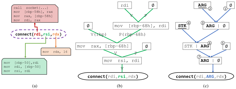
Figure 2. Creating pointer-aware slices for extracting concrete values or abstract values: all possible computations that create the value of the rsi are statically analyzed, and finally, the occurrence of rsi in the call to connect is replaced with the ARG abstract value originating from \raisebox{0pt}{\footnotesize{2}}⃝, which is defined as more informative than $\emptyset$ (\raisebox{0pt}{\footnotesize{1}}⃝) and STK (\raisebox{0pt}{\footnotesize{4}}⃝).

Analyzing slice trees We analyze slice trees to select a concrete value or an abstract value to replace the register name in the sink of the tree. To do this, we need to assign abstract values to some of the slice tree leaves, and propagate the values in the tree.

We begin by performing the following initial tag assignments in the tree:

• The arguments accepted by $P$ receive the “ARG” tag.

• All call instructions receive with the “RET” tag. Note that this tag will allways be propagated to a rax register as it holds the return value of the called procedure.

• The rbp register at the beginning of $P$ receives the “STK” tag. During the propagation process, this tag might be passed to rsp or other registers.

• When a pointer to a global value can not be resolved to a concrete value, e.g., a number or a string, this pointer receive the “GLOBAL” tag.

After this initial tag assignment, we propagate values downwards in the tree towards the register at the tree sink. We prefer values according to the following order: (1) concrete value, (2) ARG, (3) GLOBAL, (4) RET, (5) STK. This hierarchy represents the certainty level we have regarding a specific value: if the value was created by another procedure – there is no information about it; if the value was created using one of $P$’s arguments, we have some information about it; and if the concrete value is available – it is used instead of an abstract value. To make this order complete, we add (6) $\emptyset$ (empty set), but this tag is never propagated forward over any other tag, and in no case will reach the sink. This ordering is required to resolve cases in which two tags are propagated into the same node. An example for such a case is shown in the following example.

Figure 2(c) shows an example of this propagation process:

1. The assigned tags “ARG” and “STK” in \raisebox{0pt}{\footnotesize{2}}⃝ and \raisebox{0pt}{\footnotesize{4}}⃝, accordingly, are marked in bold and underlined.

2. Two tags, “ARG” and “$\emptyset$” are propagated to \raisebox{0pt}{\footnotesize{3}}⃝, and “ARG”, marked in bold, is propagated to \raisebox{0pt}{\footnotesize{6}}⃝.

3. In \raisebox{0pt}{\footnotesize{6}}⃝, as “ARG” is preferred over “STK”, “ARG”, marked again in bold, is propagated to \raisebox{0pt}{\footnotesize{7}}⃝.

4. From \raisebox{0pt}{\footnotesize{6}}⃝ “ARG”, in bold, is finally propagated to the sink and thus selected to replace the rdi register name in the connect call site.

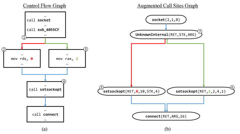
Figure 3. An example of a CFG and the augmented call site graph created by analyzing it using our approach

An augmented call site graph example Fig. 3 shows an example of a CFG and the augmented call site graph, henceforth augmented graph for short, created by analyzing it using our approach.

Node \raisebox{0pt}{\footnotesize{4}}⃝ from the CFG is represented by two nodes in the augmented graph: \raisebox{0pt}{\footnotesize{5}}⃝ and \raisebox{0pt}{\footnotesize{6}}⃝. This is the result of two different paths in the CFG leading into the call instruction call setsockopt: \raisebox{0pt}{\footnotesize{1}}⃝$\rightarrow$\raisebox{0pt}{\footnotesize{2}}⃝$\rightarrow$\raisebox{0pt}{\footnotesize{4}}⃝ and \raisebox{0pt}{\footnotesize{1}}⃝$\rightarrow$\raisebox{0pt}{\footnotesize{3}}⃝$\rightarrow$\raisebox{0pt}{\footnotesize{4}}⃝. In each path, the values building the augmented call site are different due to the different slices created for the same registers used as arguments in each path. One such difference is the second argument of setsockopt being a (red) $0$ in \raisebox{0pt}{\footnotesize{5}}⃝ and a (green) $1$ in \raisebox{0pt}{\footnotesize{6}}⃝.

Also note that internal procedure calls, while missing the target procedure name, which is marked by “UnknownInternal” in \raisebox{0pt}{\footnotesize{7}}⃝, is part of the augmented graph and thus contribute to the representation of $P$.

Dealing with aliasing and complex constant expressions Building upon our previous work, David et al. (2017), we re-optimize the entire procedure and re-optimize every slice before analyzing it to deduce argument values. A complex calculation of constants is thus replaced by the re-optimization process. For example, the instructions xor rax,rax; inc rax; are simply replaced to mov rax,1. This saves us from performing the costly process of expression simplification and the need to expand our analysis to support them.

Furthermore, although very common in (human written) source code – memory aliasing is seldom performed in optimized binary code, as it contradict the compiler’s aspiration for reducing memory consumption and avoiding redundant computations. An example for how aliasing is avoided is depicted in the lower left (green) slice in Fig. 2(a): an offset to the stack storing a local variable can always be addressed in the same way using rbp (in this case, rbp-50h). The re-optimization thus frees us from expanding our analysis to address memory aliasing.

Facilitating augmented call site graphs creation To efficiently analyze procedures with a sizable CFGs (i.e., a large number of basic blocks and edges) we apply a few optimizations: (i) cache value computation for path prefixes; (ii) merge sub-paths if they do not contain calls; (iii) remove duplicate sequences; and (iv) as all call instructions are replaced with the “RET” label, we do not continue the slicing operation after encountering call commands.

5. Model

The key idea in this work is to represent a binary procedure as structured call sites, and the novel synergy between program analysis of binaries and neural models, rather than the specific neural architecture. In Section 6, we experiment with plugging in our representation into LSTMs, Transformers, and GCNs. In Section 5.1 we describe how a call site is represented in the model; this encoding is performed similarly across architectures. We use the same encoding in three different popular architectures - LSTM-based attention encoder-decoder (Section 5.2), a Transformer (Section 5.3), and a GNN (Section 5.4).

5.1. Call Site Encoder

We define a vocabulary of learned embeddings $E^{names}$. This vocabulary assigns a vector for every subtoken of an API name that was observed in the training corpus. For example, if the training corpus contains a call to open_file, each of open and file is assigned a vector in $E^{names}$.

Additionally, we define a learned embedding for each abstract value, e.g., ARG, STK, RET and GLOBAL (Section 4), and for every actual value (e.g., the number “1”) that occurred in training data. We denote the matrix containing these vectors as $E^{values}$. We represent a call site by summing the embeddings of its API subtokens $w_{1}...w_{k_{s}}$, and concatenating with up to $k_{args}$ of argument abstract value embeddings:

$$encode\_callsite\left(w_{1}...w_{k_{s}},value_{1},...,value_{k_{args}}\right)=\left[\left(\sum_{i}^{k_{s}}E^{names}_{w_{i}}\right)\;;\;E^{values}_{value_{1}}\;;\;...\;;\;E^{values}_{{value_{k_{args}}}}\right]$$

We pad the remaining of the $k_{args}$ argument slots with an additional no-arg symbol.

5.2. Encoding Call Site Sequences with LSTMs

In LSTMs and Transformers, we extract all paths between $Entry$ and $Sink$ (Section 4) and use this set of paths to represent the procedure. We follow the general encoder-decoder paradigm (Cho et al., 2014; Sutskever et al., 2014) for sequence-to-sequence (seq2seq) models, with the difference being that the input is not the standard single sequence of symbols, but a set of call site sequences. Thus, these models can be described as “set-of-sequences-to-sequence”. We learn sequences of encoded call sites; finally, we decode the target procedure name word-by-word while considering a dynamic weighted average of encoded call site sequence vectors at each step.

In the LSTM-based model, we learn a call site sequence using a bidirectional LSTM. We represent each call site sequence by concatenating the last states of forward and backward LSTMs:

$$h_{1},...,h_{l}=LSTM_{encoder}\left(callsite_{1},...,callsite_{l}\right)$$

$$z=\left[h_{l}^{\rightarrow};h_{l}^{\leftarrow}\right]$$

Where $l$ is the maximal length of a call site sequence. In our experiments, we used $l=60$. Finally, we represent the entire procedure as a set of its encoded call site sequences $\left\{z_{1},z_{2},...,z_{n}\right\}$, which is passed to the LSTM decoder as described in Section 3.2.

5.3. Encoding Call Site Sequences with Transformers

In the Transformer model, we encode each call site sequence separately using $N$ Transformer-encoder layers, followed by attention pooling to represent a call site sequence as a single vector:

$$z=\text{Transformer}_{encoder}\left(callsite_{1},...,callsite_{l}\right)$$

Finally, we represent the entire procedure as a set of its encoded call site sequences $\left\{z_{1},z_{2},...,z_{n}\right\}$, which is passed to the Transformer-decoder as described in Section 3.3.

5.4. Encoding Call Site Sequences with Graph Neural Networks

In the GNN model, we model the entire processed CFG as a graph. We learn the graph using a graph convolutional network (GCN) (Kipf and Welling, 2017).

We begin with a graph that is identical to the CFG, where nodes are CFG basic blocks. A basic block in the CFG contains multiple call sites. We thus split each basic block to a chain of its call sites, such that all incoming edges are connected to the first call site, and the last call site is connected to all the basic block’s outgoing edges.

In a given call site in our analysis, the concrete and abstract values (Section 4) depend on the CFG path that “arrives” to the call site. In other words, the same call site argument can be assigned two different abstract values in two different runtime paths. We thus duplicate each call site that may have different combination of abstract values into multiple parallel call sites. All these duplicates contain the same API call, but with a different combination of possible abstract values. Note that while these values were deduced in the context of simple paths extracted from the CFG, here they are placed inside a graph which contains loops and other non-simple paths.

6. Evaluation

We implemented our approach in a framework called Nero, for NEural Reverse engineering Of stripped binaries.

6.1. Experimental Setup

To demonstrate how our representation can be plugged into various architectures, we implemented our approach in three models: Nero-LSTM encodes the control-flow sequences using bidirectional LSTMs and decodes with another LSTM; Nero-Transformer encodes these sequences and decodes using a Transformer (Vaswani et al., 2017); Nero-GNN encodes the CFG of augmented call sites using a GCN, and attends to the final node representations while decoding using an LSTM.

The neural architecture of Nero-LSTM is similar to the architecture of code2seq (Alon et al., 2019a), with the main difference that Nero-LSTM is based on sequences of augmented call sites, while code2seq uses sequences of AST nodes.

Creating a dataset We focus our evaluation on Intel 64-bit executables running on Linux, but the same process can be applied to other architectures and operating systems. We collected a dataset of software packages from the GNU code repository containing a variety of applications such as networking, administrative tools, and libraries.

To avoid dealing with mixed naming schemes, we removed all packages containing a mix of programming languages, e.g., a Python package containing partial C implementations.

Avoiding duplicates Following Lopes et al. (2017) and Allamanis (2018), who pointed out the existence of code duplication in open-source datasets and its adverse effects, we created the train, validation and test sets from completely separate projects and packages. Additionally, we put much effort, both manual and automatic, into filtering duplicates from our dataset. To filter duplicates, we filtered out the following:

1. Different versions of the same package – for example, “wget-1.7” and “wget-1.20”.

2. C++ code – C++ code regularly contains overloaded procedures; further, class methods start with the class name as a prefix. To avoid duplication and name leakage, we filtered out all C++ executables entirely.

3. Tests – all executables suspected as being tests or examples were filtered out.

4. Static linking – we took only packages that could compile without static linking. This ensures that dependencies are not compiled into the dependent executable.

Detecting procedure boundaries Executables are composed from sections, and, in most cases, all code is placed in one of these sections, dubbed the code section. Stripped executables do not contain information regarding the placement of procedures from the source-code in the code section. Moreover, in optimized code, procedures can be in-lined or split into chunks and scattered across the code section. Executable static analysis tools employ a linear sweep or recursive descent to detect procedure boundaries.

Shin et al. (2015); Bao et al. (2014) show that modern executable static analysis tools achieve very high accuracy (~94%) in detecting procedure boundaries, yet some misses exist. While we consider detecting procedure boundaries as an orthogonal problem to procedure name prediction, we wanted our evaluation to reflect the real-world scenario. With this in mind, we employed IDAPRO, which uses recursive descent, as our initial method of detecting procedure boundaries. Then, during our process of analyzing the procedure towards extracting our augmented call-site based representation, we perform a secondary check of each procedure to make sure data-flow paths and treatment of stack frames are coherent. This process revealed some errors in IDAPRO’s boundary detection. Some were able to be fixed while others were removed from our dataset. One example of such error, which could be detected and fixed, is a procedure calling exit(). In this case, no stack clean-up or ret instruction is put after the call, and the following instructions belong to another procedure. We note that without debug information, in-lined procedures are not detected and thus cannot have their name predicted.

Comparing the boundaries that are automatically detected by this process with the debug information generated during compilation – showed that less than $1\%$ of the procedures suffered from a boundary detection mistake. These errors resulted in short pieces of code that were moved from one procedure into another or causing a new procedure to be created. Following our desire to simulate a real-world scenario we kept all of these procedures in our dataset.

Obfuscating API names A common anti-RE technique is obfuscation of identities of APIs being used by the executable. Tools that implement this technique usually perform the following:

1. Modify the information that is stored inside sections of the executable in order to break the connections between calls targeting imported procedures and the imported procedure.

2. Add code in the beginning of the executable’s execution to mimic the OS loader and re-create these connections at runtime.

The obstructive actions of the first step ((1)) also affect automatic static analysis tools such as ours. Specifically, the process of reconstructing call sites for external calls (described in Section 4) will be disrupted. While the number of arguments can still be computed by analyzing the calling procedure, the API names can not be resolved, as the semantics of the call and argument preparation must remain intact.

In our evaluation, we wanted to test the performance of our approach in the presence of such API name obfuscation. To simulate API name obfuscation tools we removed the most important information used by the dynamic loader, the name of (or path to) the files to load, and which of the procedures in them are called by the executable. All of this information is stored in the .dynstr section, as a list of null-character separated strings. Replacing the content of this section with nulls (zeros) will hinder its ability to run, yet we made sure that after these manipulations Nero would still be able to analyze the executable correctly.

Dataset processing and statistics After applying all filtering, our dataset contains $67,246$ examples. We extracted procedure names to use as labels, and then created two datasets by: (i) stripping, and (ii) stripping and obfuscating API names (the API name obfuscation is described above.)

We split both datasets into the same training-validation-test sets using a $(8:1:1)$ ratio resulting in 60403/2034/4809 training/validation/test examples. Each dataset contains $2.42\left(\pm 0.04\right)$ target symbols per example. There are $\textbf{489.63}\left(\pm 2.82\right)$ assembly code tokens per procedure, which our analysis reduces to $5.6\left(\pm 0.03\right)$ nodes (in GNN); $9.05\left(\pm 0.18\right)$ paths per procedure (in LSTMs and Transformers); the average path is $9.15\left(\pm 0.01\right)$ call sites long. Our datasets are publicly available at https://github.com/tech-srl/Nero.

Procedures that do not have any API calls, but still have internal calls, can still benefit from our augmented call site representation. These constitute 15% of our benchmark.

Metrics At test and validation time, we adopted the measure used by previous work (Allamanis et al., 2016; Alon et al., 2019a; Fernandes et al., 2019), and measured precision, recall and F1 score over the target subtokens, case-, order-, and duplication-insensitive, and ignoring non-alphabetical characters. For example, for a true reference of open file: a prediction of open is given full precision and $50\%$ recall; and a prediction of file open input file is given $67\%$ precision and full recall.

Baselines We compare our models to the state-of-the-art, non-neural, model Debin (He et al., 2018). This is a non-neural baseline based on Conditional Random Fields (CRFs). We note that Debin was designed for a slightly different task of predicting names for both local variables and procedure names. Nevertheless, we focus on the task of predicting procedure names and use only these to compute their score. The authors of Debin (He et al., 2018) offered their guidance and advice in performing a fair comparison, and they provided additional evaluation scripts.

DIRE (Lacomis et al., 2019) is a more recent work, which creates a representation for binary procedure elements based on Hex-Rays, a black-box commercial decompiler. One part of the representation is based on a textual output of the decompiler – a sequence of C code tokens, that is fed to an LSTM. The other part is an AST of the decompiled C code, created by the decompiler as well, that is fed into a GNN. DIRE trains the LSTM and the GNN jointly. DIRE addresses a task related to ours – predicting names for local variables. We therefore adapted DIRE to our task of predicting procedure names by modifying the authors’ original code to predict procedure names only.

We have trained and tested the Debin and DIRE models on our dataset. As in Nero , we verified that our API name obfuscation method does prevent Debin and DIRE from analyzing the executables correctly.

Other straightforward baselines are Transformer-text and LSTM-text in which we do not perform any program analysis, and instead just apply standard NMT architectures directly on the assembly code: one is the Transformer which uses the default hyperparameters of Vaswani et al. (2017), and the other has two layers of bidirectional LSTMs with 512 units as the encoder, two LSTM layers with 512 units in the decoder, and attention (Luong et al., 2015).

Training We trained our models using a single Tesla V100 GPU. For all our models (Nero-LSTM, Nero-Transformer and Nero-GNN), we used embeddings of size $128$ for target subtokens and API subtokens, and the same size for embedding argument abstract values. In our LSTM model, to encode call site sequences, we used bidirectional LSTMs with $128$ units each; the decoder LSTM had $256$ units. We used dropout (Srivastava et al., 2014) of $0.5$ on the embeddings and the LSTMs. For our Transformer model we used $N=6$ encoder layers and the same number of decoder layers, keys and values of size $d_{k}=d_{v}=32$, and a feed-forward network of size $128$. In our GCN model we used 4 layers, by optimizing this value on the validation set; larger values showed only minor improvement. For all models, we used the Adam (Kingma and Ba, 2014) optimization algorithm with an initial learning rate of $10^{-4}$ decayed by a factor of $0.95$ every epoch. We trained each network end-to-end using the cross-entropy loss. We tuned hyperparameters on the validation set, and evaluated the final model on the test set.

	Stripped				Stripped & Obfuscated API calls
Model	Precision	Recall	F1		Precision	Recall	F1
LSTM-text	22.32	21.16	21.72		15.46	14.00	14.70
Transformer-text	25.45	15.97	19.64		18.41	12.24	14.70
Debin (He et al., 2018)	34.86	32.54	33.66		32.10	28.76	30.09
DIRE (Lacomis et al., 2019)	38.02	33.33	35.52		23.14	25.88	24.43
Nero-LSTM	39.94	38.89	39.40		39.12	31.40	34.83
Nero-Transformer	41.54	38.64	40.04		36.50	32.25	34.24
Nero-GNN	48.61	42.82	45.53		40.53	37.26	38.83

Table 2. Our models outperform previous work, DIRE and Debin , by a relative improvement of $28\%$ and $35\%$ resp.; learning from the flat assembly code (LSTM-text, Transformer-text) yields much lower results. Obfuscating API calls hurts all models, but thanks to the use of abstract and concrete values, our model still performs better than the baselines.

6.2. Results

The left side of Table 2 shows the results of the comparison to Debin, DIRE, LSTM-text, and Transformer-text on the stripped dataset. Overall, our models outperform all the baselines. This shows the usefulness of our representation with different learning architectures.

Nero-Transformer performs similarly to Nero-LSTM, while Nero-GNN performs better than both. Nero-GNN show $28\%$ relative improvement over DIRE, $35\%$ over Debin, and over $100\%$ relative gain over LSTM-text and Transformer-text.

The right side of Table 2 shows the same models on the stripped and API-obfuscated dataset. Obfuscation degrades the results of all models, yet our models still outperform DIRE , Debin, and the textual baselines. These results depict the importance of augmenting call sites using abstract and concrete values in our representation, which can recover sufficient information even in the absence of API names. We note that overall, in both datasets, our models perform best on both precision, recall, and F1.

Comparison to Debin  Conceptually, our model is much more powerful than the model of Debin because it is able to decode out-of-vocabulary procedure names (“neologisms”) from subtokens, while the CRF of Debin uses a closed vocabulary that can only predict already-seen procedure names. At the binary code side, since our model is neural, at test time it can utilize unseen call site sequences while their CRF can only use observed relationships between elements. For a detailed discussion about the advantages of neural models over CRFs, see Section 5 of (Alon et al., 2019c). Furthermore, their representation performs a shallow translation from binary instruction to connections between symbols, while our representation is based on a deeper data-flow-based analysis to find values of registers arguments of imported procedures.

Comparison to DIRE  The DIRE model and our Nero-GNN model use similar neural architectures; yet, our models perform much better. While decompilation evolves static analysis, its goal is to generate human readable output. On the other hand, our representation was tailor made for the prediction task, by focusing on the call sites and augmenting them to encode more information.

Comparison to LSTM-text and Transformer-text The comparison to the NMT baselines shows that learning directly from the assembly code performs significantly worse than leveraging semantic knowledge and static analysis of binaries. We hypothesize that the reasons are the high variability in the assembly data, which results in a low signal-to-noise ratio. This comparison necessitates the need of an informative static analysis to represent and learn from executables.

Model	Prediction
Ground truth	locate unset	free words	get user groups	install signal handlers
Debin	var is unset	search	display	signal setup
DIRE	env concat	restore	prcess file	overflow
LSTM-text	url get arg	func free	¡unk¿	¡unk¿
Transformer-text	¡unk¿	¡unk¿	close stdin	¡unk¿
Nero-LSTM	var is unset	quotearg free	get user groups	enable mouse
Nero-Transformer	var is unset	quotearg free	open op	¡empty¿
Nero-GNN	var is unset	free table	get user groups	signal enter handlers

Table 3. Examples from our test set and predictions made by the different models. Even when a prediction is not an “exact match” to the ground truth, it usually captures more subtokens of the ground truth than the baselines. More examples can be found in Appendix A.

Examples Table 3 shows a few examples for predictions made by the different models. Additional examples can be found in Appendix A.

6.3. Ablation study

To evaluate the contribution of different components of our representation, we compare the following configurations:

Nero-LSTM no values - uses only the CFG analysis with the called API names, without abstract nor concrete values, and uses the LSTM-based model.

Nero-Transformer no values - uses only the CFG analysis with the called API names, without abstract nor concrete values, and uses the Transformer-based model.

Nero-GNN no-values - uses only the CFG analysis without abstract nor concrete values, and uses the GNN-based model.

Nero-LSTM no-library-debug - does not use debug information for external dependencies when reconstructing call sites, and uses the LSTM-based model.

Nero-Transformer no-library-debug - does not use debug information for external dependencies when reconstructing call sites, and uses the Transformer-based model.

Nero-GNN no-library-debug - does not use debug information for external dependencies when reconstructing call sites, and uses the GNN-based model.

Nero Transformer$\rightarrow$LSTM - uses a Transformer to encode the sets of control-flow sequences and an LSTM to decode the prediction.

BiLSTM call sites - uses the same enriched call sites representation as our model including abstract values, with the main difference being that the order of the call sites is their order in the assembly code: there is no analysis of the CFG.

BiLSTM calls - does not use CFG analysis or abstract values. Instead, it uses two layers of bidirectional LSTMs with attention to encode call instructions with only the name of the called procedure, in the order they appear in the executable.

Results Table 4 shows the performance of the different configurations. Nero-LSTM achieves  $50\%$ higher relative score than Nero-LSTM no-values; Nero-GNN achieves $20\%$ higher relative score than Nero-GNN no-values. This shows the contribution of the call site augmentation by capturing values and abstract values and its importance to prediction.

The no-library-debug variations of each model achieve comparable results to the originals (which using the debug information from the libraries). These results showcase the precision of our analysis and its applicability to possible real-world scenarios in which library code is present without debug information.

Nero Transformer$\rightarrow$LSTM achieved slightly lower results to Nero-Transformer and Nero-LSTM. This shows that the representation and the information that is captured in it – affect the results much more than the specific neural architecture.

As we discuss in Section 4, our data-flow-based analysis helps filtering and reordering calls in their approximate chronological runtime order, rather than the arbitrary order of calls as they appear in the assembly code. BiLSTM call sites performs slightly better than BiLSTM calls due to the use of abstract values instead of plain call instructions. Nero-LSTM improves over BiLSTM call sites by 16%, showing the importance of learning call sites in their right chronological order and the importance of our data-flow-based observation of executables.

Model	Prec	Rec	F1
BiLSTM calls	23.45	24.56	24.04
BiLSTM call sites	36.05	31.77	33.77
Nero-LSTM no-values	27.22	23.91	25.46
Nero-Transformer no-values	29.84	24.08	26.65
Nero-GNN no-values	45.20	32.65	37.91
Nero-LSTM no-library-debug	39.51	40.33	39.92
Nero-Transformer no-library-debug	43.60	37.65	40.44
Nero-GNN no-library-debug	47.73	42.82	45.14
Nero Transformer$\rightarrow$LSTM	39.05	36.47	37.72
Nero-LSTM	39.94	38.89	39.40
Nero-Transformer	41.54	38.64	40.04
Nero-GNN	48.61	42.82	45.53

Table 4. Variations on our models that ablate different components.

6.4. Qualitative evaluation

Taking a closer look at partially-correct predictions reveals some common patterns. We divide these partially-correct predictions into major groups; Table 5 shows a few examples from interesting and common groups.

The first group, “Programmers VS English Language”, depicts prediction errors that are caused by programmers’ naming habits. The first two lines of Table 5 show an example of a relatively common practice for programmers – the use of shorthands. In the first example, the ground truth is i18n_initialize; yet the model predicts the shorthand init. In the second example, the ground truth subtoken is the shorthand cfg but the model predicts config. We note that cfg, config and init appear $81$, $496$ and $6808$ times, respectively, in our training set. However, initialize does not appear at all, thus justifying the model’s prediction of init.

In the second group, “Data Structure Name Missing”, the model, not privy to application-specific labels that exist only in the test set, resorts to predicting generic data structures names (i.e., a list). That is, instead of predicting the application-specific structure, the model predicts the most similar generic data structure in terms of common memory and API use-patterns. In the first example, speed records are predicted as list items. In the next example, the parsing of a (windows) directories, performed by the wget package, is predicted as parsing a tree. In the last example, the subtoken gzip is out-of-vocabulary, causing abort_gzip to be predicted instead as fatal.

The last group, “Verb Replacement”, shows how much information is captured in verbs of procedure name. In the first example, share is replaced with add, losing some information about the work performed in the procedure. In the last example, display is replaced with show, which are almost synonymous.

Error Type	Package	Ground Truth	Predicted Name
Programmers VS English Language	wget	i18n_initialize	i18n_init
	direvent	split_cfg_path	split_config_path
	gzip	add_env_opt	add_option
Data Structure Name Missing	gtypist	get_best_speed	get_list_item
	wget	ftp_parse_winnt_ls	parse_tree
	direvent	filename_pattern_free	free_buffer
	gzip	abort_gzip_signal	fatal_signal_handler
Verb Replacement	findutils	share_file_fopen	add_file
	units	read_units	parse
	wget	retrieve_from_file	get_from_file
	mcsim	display_help	show_help

Table 5. Examination of common interesting model mistakes.

6.5. Limitations

In this section, we focus on the limitations in our approach, which could serve as a basis for future research.

Heavy obfuscations and packers In our evaluation, we explored the effects of API obfuscation and show that they cause a noticeable decrease in precision for all name prediction models reviewed (Section 6.2). Alternatively, there are more types of obfuscators, packers, and other types of self-modifying code. Addressing these cases better involves detecting them at the static analysis phase and employing other methods (e.g., Edmonds (2006)) before attempting to predict procedure names.

Representation depending on call sites As our representation for procedures is based on call site reconstruction and augmentation, it is dependent on the procedure having at least one call site and the ability to detect them statically.

Moreover, as we mentioned above, $15\%$ of the procedures in our dataset contain only internal calls. These are small procedures with an average of 4 (internal or indirect) calls and 10 basic blocks. These procedures are represented only by call sites of internal and indirect calls. These call sites are composed of a special “UNKNOWN” symbol with the abstract or concrete values. Predictions for these procedures receive slightly higher results - $46.26$, $49.54$, $47.84$ (Precision, Recall, F1). This is consistent with our general observation that smaller procedures are easier to predict.

Predicting names for C++ or python extension modules There is no inherent limitation in Nero preventing it from predicting class or class method names. In fact, training on C++ code only and incorporating more information available in C++ compiled binaries (as shown in (Katz et al., 2018)) in our representation makes for great material for future work. Python extension modules contain even more information as the python types are created and manipulated by calling to the python C C++ API (e.g., _PyString_FromString).

We decided to focus on binaries created from C code because they contain the smallest amount of information and because this was also done in other works that we compared against (He et al. (2018); Lacomis et al. (2019)).

7. Related Work

Machine learning for source code Several works have investigated machine learning approaches for predicting names in high-level languages. Most works focused on variable names (Alon et al., 2018; Bavishi et al., 2018), method names (Allamanis et al., 2016; Alon et al., 2019c; Allamanis et al., 2015a) or general properties of code (Raychev et al., 2016b, 2014). Another interesting application is measuring the likelihood of existing names to detect naming bugs (Pradel and Sen, 2018; Rice et al., 2017). Most work in this field used either syntax only (Bielik et al., 2016; Raychev et al., 2016a; Maddison and Tarlow, 2014), semantic analysis (Allamanis et al., 2018) or both (Raychev et al., 2015; Iyer et al., 2018). Leveraging syntax only may be useful in languages such as Java and JavaScript that have a rich syntax, which is not available in our difficult scenario of RE of binaries. In contrast with syntactic-only work such as Alon et al. (2019a, c), working with binaries requires a deeper semantic analysis in the spirit of Allamanis et al. (2018), which recovers sufficient information for training the model using semantic analysis.

Allamanis et al. (2018), Brockschmidt et al. (2019) and Fernandes et al. (2019) further leveraged semantic analysis with GNNs, where edges in the graph were relations found using syntactic and semantic analysis. Another work (DeFreez et al., 2018) learned embeddings for C functions based on the CFG. We also use the CFG, but in the more difficult domain of stripped compiled binaries rather than C code.

Static analysis models for RE Debin (He et al., 2018) used static analysis with CRFs to predict various properties in binaries. As we show in Section 6, our model gains $20\%$ higher accuracy due to Debin’s sparse model and our deeper data-flow analysis.

In a concurrent work with ours, DIRE (Lacomis et al., 2019) addresses name prediction for local variables in binary procedures. Their approach relies on a commercial decompiler and its evaluation was performed only on non-stripped executables. Our approach works directly on the optimized binaries. Moreover, they focused on predicting variable names, which is more of a local prediction; in contrast, we focus on predicting procedure names, which requires a more global view of the given binary. Their approach combines an LSTM applied on the flat assembly code with a graph neural network applied on the AST of the decompiled C code, without a deep static analysis as in ours and without leveraging the CFG. Their approach is similar to the LSTM-text baseline combined with the Nero-LSTM no-values ablation. As we show in Section 6, our GNN-based model achieves $28\%$ higher scores thanks to our deeper data-flow analysis.

Static analysis frameworks for RE Katz et al. (2018) showed an approach to infer subclass-superclass relations in stripped binaries. Lee et al. (2011) used static and dynamic analysis to recover high-level types. In contrast, our approach is purely static. (Reps et al., 2005) presented CodeSurfer, a binary executable framework built for analyzing x86 executables, focusing on detecting and manipulating variables in the assembly code. Shin et al. (2015); Bao et al. (2014) used RNNs to identify procedure boundaries inside a stripped binary.

Similarity in binary procedures David et al. (2017) and Pewny et al. (2015) addressed the problem of finding similar procedures to a given procedure or executable, which is useful to detect vulnerabilities. Xu et al. (2017) presents Gemini, a deep nural network (DNN) based model for establishing binary similarity. Gemini works by annotating CFG with manually selected features, and using them to create embeddings for basic blocks and create a graph representation. This representation is then fed into a Siamese architecture to generate a similarity label (similar or not similar). Ding et al. (2019) propused Asm2Vec. Asm2Vec works by encoding assembly code and the CFG into a feature vector and using a PV-DM based model to compute similarity.

8. Conclusion

We present a novel approach for predicting procedure names in stripped binaries. The core idea is to leverage static analysis of binaries to encode rich representations of API call sites; use the CFG to approximate the chronological runtime order of the call sites, and encode the CFG using either a set of sequences or a graph, using three different neural architectures (LSTM-based, Transformer-based, and graph-based).

We evaluated our framework on real-world stripped procedures. Our model achieves a $35\%$ relative gain over existing non-neural approaches, and more than a $100\%$ relative gain over the naïve textual baselines (“LSTM-text”, “Transformer-text” and DIRE). Our ablation study shows the importance of analyzing argument values and learning from the CFG. To the best of our knowledge, this is the first work to leverage deep learning for reverse engineering procedure names in binary code.

We believe that the principles presented in this paper can serve as a basis for a wide range of tasks that involve learning models and RE, such as malware and ransomware detection, executable search, and neural decompilation. To this end, we make our dataset, code, and trained models publicly available at https://github.com/tech-srl/Nero.

Acknowledgements

We would like to thank Jingxuan He and Martin Vechev for their help in running Debin, and Emery Berger for his useful advice. We would also like to thank the anonymous reviewers for their useful suggestions.

The research leading to these results has received funding from the Israel Ministry of Science and Technology, grant no. 3-9779.

Appendix A Additional Examples

Table 6 contains more examples from our test set, along with the predictions made by our model and each of the baselines.

Ground Truth	He et al. (2018)	LSTM-text	Transformer-text	BiLSTM call-sites	Nero-LSTM
mktime from utc	nettle pss …	get boundary	¡unk¿	str file	mktime
read buffer	concat	fopen safer	mh print fmtspec	net read	filter read
get widech	get byte	user	mh decode rcpt flag	¡unk¿	do tolower
ftp parse winnt ls	uuconf iv …	mktime	print status	send to file	parse tree
write init pos	allocate pic buf	open int	¡unk¿	print type	cfg init
wait for proc	wait subprocess	start open	mh print fmtspec	¡unk¿	strip
read string	cmp	error	check command	process	io read
find env	find env pos	proper name utf	close stream	read token	find env
write calc jacob	usage msg	update pattern	print one paragraph	¡unk¿	write
write calc outputs	fsquery show	debug section	cwd advance fd	¡unk¿	write
get script line	get line	make dir hier	¡unk¿	read ps line	jconfig get
getuser readline	stdin read readline	rushdb print	mh decode rcpt flag	write line	readline read
set max db age	do link	set owner	make dir hier	sparse copy	set
write calc deriv	orthodox hdy	ds symbol	close stream	fprint entry	write type
read file	bt open	¡unk¿	… disable coredump	¡unk¿	vfs read file
parse options	parse options	finish	mh print fmtspec	get options	parse args
url free	hash rehash	hostname destroy	setupvariables	hol free	free dfa content
check new watcher	read index	check opt	¡unk¿	open source	check file
open input file	get options	query in	ck rename	set	delete input
write calc jacob	put in fp table	save game var	hostname destroy	¡unk¿	write
filename pattern free	add char segment	free dfa content	hostname destroy	glob cleanup	free exclude segment
read line	tartime	init all	close stdout	parse args	read
ftp parse unix ls	serv select fn	canonicalize	¡unk¿	¡unk¿	parse syntax option
free netrc	gea compile	hostname destroy	hostname destroy	free ent	hol free
string to bool	string to bool	setnonblock	mh decode rcpt flag	string to bool	string to bool

Table 6. Examples from our test set and predictions made by the different models.

References

- (1)
- Alammar ([n. d.]) Jay Alammar. [n. d.]. The Illustrated Transformer. http://jalammar.github.io/illustrated-transformer/.
- Allamanis (2018) Miltiadis Allamanis. 2018. The Adverse Effects of Code Duplication in Machine Learning Models of Code. arXiv preprint arXiv:1812.06469 (2018).
- Allamanis et al. (2015a) Miltiadis Allamanis, Earl T. Barr, Christian Bird, and Charles Sutton. 2015a. Suggesting Accurate Method and Class Names. In Proceedings of the 2015 10th Joint Meeting on Foundations of Software Engineering (ESEC/FSE 2015). ACM, New York, NY, USA, 38–49. https://doi.org/10.1145/2786805.2786849
- Allamanis et al. (2018) Miltiadis Allamanis, Marc Brockschmidt, and Mahmoud Khademi. 2018. Learning to Represent Programs with Graphs. In ICLR.
- Allamanis et al. (2016) Miltiadis Allamanis, Hao Peng, and Charles A. Sutton. 2016. A Convolutional Attention Network for Extreme Summarization of Source Code. In Proceedings of the 33nd International Conference on Machine Learning, ICML 2016, New York City, NY, USA, June 19-24, 2016. 2091–2100. http://jmlr.org/proceedings/papers/v48/allamanis16.html
- Allamanis et al. (2015b) Miltiadis Allamanis, Daniel Tarlow, Andrew D. Gordon, and Yi Wei. 2015b. Bimodal Modelling of Source Code and Natural Language. In Proceedings of the 32nd International Conference on International Conference on Machine Learning - Volume 37 (ICML’15). JMLR.org, 2123–2132. http://dl.acm.org/citation.cfm?id=3045118.3045344
- Alon et al. (2019a) Uri Alon, Shaked Brody, Omer Levy, and Eran Yahav. 2019a. code2seq: Generating Sequences from Structured Representations of Code. In International Conference on Learning Representations. https://openreview.net/forum?id=H1gKYo09tX
- Alon et al. (2019b) Uri Alon, Roy Sadaka, Omer Levy, and Eran Yahav. 2019b. Structural Language Models for Any-Code Generation. arXiv preprint arXiv:1910.00577 (2019).
- Alon et al. (2018) Uri Alon, Meital Zilberstein, Omer Levy, and Eran Yahav. 2018. A General Path-based Representation for Predicting Program Properties. In Proceedings of the 39th ACM SIGPLAN Conference on Programming Language Design and Implementation (PLDI 2018). ACM, New York, NY, USA, 404–419. https://doi.org/10.1145/3192366.3192412
- Alon et al. (2019c) Uri Alon, Meital Zilberstein, Omer Levy, and Eran Yahav. 2019c. Code2Vec: Learning Distributed Representations of Code. Proc. ACM Program. Lang. 3, POPL, Article 40 (2019), 29 pages. https://doi.org/10.1145/3290353
- Bahdanau et al. (2014) Dzmitry Bahdanau, Kyunghyun Cho, and Yoshua Bengio. 2014. Neural Machine Translation by Jointly Learning to Align and Translate. CoRR abs/1409.0473 (2014). http://arxiv.org/abs/1409.0473
- Bao et al. (2014) Tiffany Bao, Jonathan Burket, Maverick Woo, Rafael Turner, and David Brumley. 2014. BYTEWEIGHT: Learning to recognize functions in binary code. Proceedings of the 23rd USENIX Security Symposium (2014), 845–860.
- Bavishi et al. (2018) Rohan Bavishi, Michael Pradel, and Koushik Sen. 2018. Context2Name: A deep learning-based approach to infer natural variable names from usage contexts. arXiv preprint arXiv:1809.05193 (2018).
- Bielik et al. (2016) Pavol Bielik, Veselin Raychev, and Martin T. Vechev. 2016. PHOG: Probabilistic Model for Code. In Proceedings of the 33nd International Conference on Machine Learning, ICML 2016, New York City, NY, USA, June 19-24, 2016. 2933–2942. http://jmlr.org/proceedings/papers/v48/bielik16.html
- Brockschmidt et al. (2019) Marc Brockschmidt, Miltiadis Allamanis, Alexander L. Gaunt, and Oleksandr Polozov. 2019. Generative Code Modeling with Graphs. In International Conference on Learning Representations. https://openreview.net/forum?id=Bke4KsA5FX
- Chiu et al. (2018) Chung-Cheng Chiu, Tara N Sainath, Yonghui Wu, Rohit Prabhavalkar, Patrick Nguyen, Zhifeng Chen, Anjuli Kannan, Ron J Weiss, Kanishka Rao, Ekaterina Gonina, et al. 2018. State-of-the-art speech recognition with sequence-to-sequence models. In 2018 IEEE International Conference on Acoustics, Speech and Signal Processing (ICASSP). IEEE, 4774–4778.
- Cho et al. (2014) Kyunghyun Cho, Bart Van Merriënboer, Caglar Gulcehre, Dzmitry Bahdanau, Fethi Bougares, Holger Schwenk, and Yoshua Bengio. 2014. Learning phrase representations using RNN encoder-decoder for statistical machine translation. arXiv preprint arXiv:1406.1078 (2014).
- David et al. (2017) Yaniv David, Nimrod Partush, and Eran Yahav. 2017. Similarity of Binaries Through Re-optimization. In Proceedings of the 38th ACM SIGPLAN Conference on Programming Language Design and Implementation (PLDI 2017). ACM, New York, NY, USA, 79–94. https://doi.org/10.1145/3062341.3062387
- DeFreez et al. (2018) Daniel DeFreez, Aditya V. Thakur, and Cindy Rubio-González. 2018. Path-based Function Embedding and Its Application to Error-handling Specification Mining. In Proceedings of the 2018 26th ACM Joint Meeting on European Software Engineering Conference and Symposium on the Foundations of Software Engineering (ESEC/FSE 2018). ACM, New York, NY, USA, 423–433. https://doi.org/10.1145/3236024.3236059
- Devlin et al. (2019) Jacob Devlin, Ming-Wei Chang, Kenton Lee, and Kristina Toutanova. 2019. BERT: Pre-training of Deep Bidirectional Transformers for Language Understanding. In Proceedings of the 2019 Conference of the North American Chapter of the Association for Computational Linguistics: Human Language Technologies, Volume 1 (Long and Short Papers). 4171–4186.
- Ding et al. (2019) Steven H H Ding, Benjamin C M Fung, and Philippe Charland. 2019. Asm2Vec : Boosting Static Representation Robustness for Binary Clone Search against Code Obfuscation and Compiler Optimization. S&P (2019), 5–6.
- Edmonds (2006) R. Edmonds. 2006. PolyUnpack : Automating the Hidden-Code Extraction of.
- Fernandes et al. (2019) Patrick Fernandes, Miltiadis Allamanis, and Marc Brockschmidt. 2019. Structured Neural Summarization. In International Conference on Learning Representations. https://openreview.net/forum?id=H1ersoRqtm
- Fowler and Beck (1999) Martin Fowler and Kent Beck. 1999. Refactoring: Improving the Design of Existing Code. Addison-Wesley Professional.
- He et al. (2018) Jingxuan He, Pesho Ivanov, Petar Tsankov, Veselin Raychev, and Martin Vechev. 2018. Debin: Predicting Debug Information in Stripped Binaries. In Proceedings of the 2018 ACM SIGSAC Conference on Computer and Communications Security (CCS ’18). ACM, New York, NY, USA, 1667–1680. https://doi.org/10.1145/3243734.3243866
- Hex-Rays ([n. d.]) Hex-Rays. [n. d.]. Hex-Rays Hex-Rays. http://www.hex-rays.com.
- Hochreiter and Schmidhuber (1997) Sepp Hochreiter and Jürgen Schmidhuber. 1997. Long Short-Term Memory. Neural Comput. 9, 8 (Nov. 1997), 1735–1780. https://doi.org/10.1162/neco.1997.9.8.1735
- Høst and Østvold (2009) Einar W. Høst and Bjarte M. Østvold. 2009. Debugging Method Names. In Proceedings of the 23rd European Conference on ECOOP 2009 — Object-Oriented Programming (Genoa). Springer-Verlag, Berlin, Heidelberg, 294–317. https://doi.org/10.1007/978-3-642-03013-0_14
- IDAPRO ([n. d.]) IDAPRO. [n. d.]. IDAPRO IDAPRO. http://www.hex-rays.com.
- Intel ([n. d.]) Intel. [n. d.]. Linux64-abi LINUXABI. https://software.intel.com/sites/default/files/article/402129/mpx-linux64-abi.pdf.
- Iyer et al. (2018) Srinivasan Iyer, Ioannis Konstas, Alvin Cheung, and Luke Zettlemoyer. 2018. Mapping Language to Code in Programmatic Context. In Proceedings of the 2018 Conference on Empirical Methods in Natural Language Processing. 1643–1652.
- Jacobson et al. (2011) Emily R. Jacobson, Nathan E. Rosenblum, and Barton P. Miller. 2011. Labeling library functions in stripped binaries. In Proceedings of the 10th SIGPLAN-SIGSOFT workshop on Program analysis for software tools, PASTE’11. 1–8. https://doi.org/10.1145/2024569.2024571
- Katz et al. (2018) Omer Katz, Noam Rinetzky, and Eran Yahav. 2018. Statistical Reconstruction of Class Hierarchies in Binaries. In Proceedings of the Twenty-Third International Conference on Architectural Support for Programming Languages and Operating Systems (ASPLOS ’18). ACM, New York, NY, USA, 363–376. https://doi.org/10.1145/3173162.3173202
- Kingma and Ba (2014) Diederik Kingma and Jimmy Ba. 2014. Adam: A method for stochastic optimization. arXiv preprint arXiv:1412.6980 (2014).
- Kipf and Welling (2017) Thomas Kipf and Max Welling. 2017. Semi-Supervised Classification with Graph Convolutional Networks. In ICLR.
- Lacomis et al. (2019) Jeremy Lacomis, Pengcheng Yin, Edward J Schwartz, Miltiadis Allamanis, Claire Le Goues, Graham Neubig, and Bogdan Vasilescu. 2019. DIRE: A Neural Approach to Decompiled Identifier Naming. arXiv preprint arXiv:1909.09029 (2019).
- Lee et al. (2011) JongHyup Lee, Thanassis Avgerinos, and David Brumley. 2011. TIE: Principled reverse engineering of types in binary programs. (2011).
- Lopes et al. (2017) Cristina V Lopes, Petr Maj, Pedro Martins, Vaibhav Saini, Di Yang, Jakub Zitny, Hitesh Sajnani, and Jan Vitek. 2017. DéjàVu: a map of code duplicates on GitHub. Proceedings of the ACM on Programming Languages 1, OOPSLA (2017), 84.
- Lu et al. (2017) Yanxin Lu, Swarat Chaudhuri, Chris Jermaine, and David Melski. 2017. Data-Driven Program Completion. CoRR abs/1705.09042 (2017). arXiv:1705.09042 http://arxiv.org/abs/1705.09042
- Luong et al. (2015) Thang Luong, Hieu Pham, and Christopher D. Manning. 2015. Effective Approaches to Attention-based Neural Machine Translation. In Proceedings of the 2015 Conference on Empirical Methods in Natural Language Processing, EMNLP 2015, Lisbon, Portugal, September 17-21, 2015. 1412–1421. http://aclweb.org/anthology/D/D15/D15-1166.pdf
- Lyle and Binkley (1993) James R Lyle and David Binkley. 1993. Program slicing in the presence of pointers. In Proceedings of the 1993 Software Engineering Research Forum. Citeseer, 255–260.
- Maddison and Tarlow (2014) Chris Maddison and Daniel Tarlow. 2014. Structured generative models of natural source code. In International Conference on Machine Learning. 649–657.
- Murali et al. (2017) Vijayaraghavan Murali, Swarat Chaudhuri, and Chris Jermaine. 2017. Bayesian Sketch Learning for Program Synthesis. CoRR abs/1703.05698 (2017). arXiv:1703.05698 http://arxiv.org/abs/1703.05698
- Pewny et al. (2015) Jannik Pewny, Behrad Garmany, Robert Gawlik, Christian Rossow, and Thorsten Holz. 2015. Cross-Architecture Bug Search in Binary Executables. In Proceedings of the 2015 IEEE Symposium on Security and Privacy (SP ’15). IEEE Computer Society, Washington, DC, USA, 709–724. https://doi.org/10.1109/SP.2015.49
- Pradel and Sen (2018) Michael Pradel and Koushik Sen. 2018. DeepBugs: A Learning Approach to Name-based Bug Detection. Proc. ACM Program. Lang. 2, OOPSLA, Article 147 (Oct. 2018), 25 pages. https://doi.org/10.1145/3276517
- RADAR ([n. d.]) RADAR. [n. d.]. Radare RADAR. https://www.radare.org/.
- Radford et al. (2018) Alec Radford, Jeffrey Wu, Rewon Child, David Luan, Dario Amodei, and Ilya Sutskever. 2018. Language models are unsupervised multitask learners. (2018).
- Raychev et al. (2016a) Veselin Raychev, Pavol Bielik, and Martin Vechev. 2016a. Probabilistic Model for Code with Decision Trees. In Proceedings of the 2016 ACM SIGPLAN International Conference on Object-Oriented Programming, Systems, Languages, and Applications (OOPSLA 2016). ACM, New York, NY, USA, 731–747. https://doi.org/10.1145/2983990.2984041
- Raychev et al. (2016b) Veselin Raychev, Pavol Bielik, Martin Vechev, and Andreas Krause. 2016b. Learning Programs from Noisy Data. In Proceedings of the 43rd Annual ACM SIGPLAN-SIGACT Symposium on Principles of Programming Languages (POPL ’16). ACM, New York, NY, USA, 761–774. https://doi.org/10.1145/2837614.2837671
- Raychev et al. (2015) Veselin Raychev, Martin Vechev, and Andreas Krause. 2015. Predicting Program Properties from ”Big Code”. In Proceedings of the 42Nd Annual ACM SIGPLAN-SIGACT Symposium on Principles of Programming Languages (POPL ’15). ACM, New York, NY, USA, 111–124. https://doi.org/10.1145/2676726.2677009
- Raychev et al. (2014) Veselin Raychev, Martin Vechev, and Eran Yahav. 2014. Code Completion with Statistical Language Models. In Proceedings of the 35th ACM SIGPLAN Conference on Programming Language Design and Implementation (PLDI ’14). ACM, New York, NY, USA, 419–428. https://doi.org/10.1145/2594291.2594321
- Reps et al. (2005) T. Reps, G. Balakrishnan, J. Lim, and T. Teitelbaum. 2005. A Next-generation Platform for Analyzing Executables. In Proceedings of the Third Asian Conference on Programming Languages and Systems (APLAS’05). Springer-Verlag, Berlin, Heidelberg, 212–229. https://doi.org/10.1007/11575467_15
- Rice et al. (2017) Andrew Rice, Edward Aftandilian, Ciera Jaspan, Emily Johnston, Michael Pradel, and Yulissa Arroyo-Paredes. 2017. Detecting argument selection defects. Proceedings of the ACM on Programming Languages 1, OOPSLA (2017), 104.
- Sachdev et al. (2018) Saksham Sachdev, Hongyu Li, Sifei Luan, Seohyun Kim, Koushik Sen, and Satish Chandra. 2018. Retrieval on source code: a neural code search. In Proceedings of the 2nd ACM SIGPLAN International Workshop on Machine Learning and Programming Languages, MAPL@PLDI 2018, Philadelphia, PA, USA, June 18-22, 2018. 31–41. https://doi.org/10.1145/3211346.3211353
- Shin et al. (2015) Eui Chul Richard Shin, Dawn Song, and Reza Moazzezi. 2015. Recognizing Functions in Binaries with Neural Networks.. In USENIX Security Symposium. 611–626.
- Srivastava et al. (2014) Nitish Srivastava, Geoffrey E Hinton, Alex Krizhevsky, Ilya Sutskever, and Ruslan Salakhutdinov. 2014. Dropout: a simple way to prevent neural networks from overfitting. Journal of machine learning research 15, 1 (2014), 1929–1958.
- Sutskever et al. (2014) Ilya Sutskever, Oriol Vinyals, and Quoc V Le. 2014. Sequence to sequence learning with neural networks. In Advances in neural information processing systems. 3104–3112.
- Vaswani et al. (2017) Ashish Vaswani, Noam Shazeer, Niki Parmar, Jakob Uszkoreit, Llion Jones, Aidan N Gomez, Łukasz Kaiser, and Illia Polosukhin. 2017. Attention is all you need. In Advances in neural information processing systems. 5998–6008.
- Votipka et al. (2020) Daniel Votipka, Seth Rabin, Kristopher Micinski, Jeffrey S Foster, and Michelle L Mazurek. 2020. An Observational Investigation of Reverse Engineers’ Processes. In 29th USENIX Security Symposium (USENIX Security 20). 1875–1892.
- Weiser (1984) Mark Weiser. 1984. Program Slicing. IEEE Transactions on Software Engineering SE-10, 4 (jul 1984), 352–357. https://doi.org/10.1109/TSE.1984.5010248
- Xu et al. (2017) Xiaojun Xu, Chang Liu, Qian Feng, Heng Yin, Le Song, and Dawn Song. 2017. Neural network-based graph embedding for cross-platform binary code similarity detection. In Proceedings of the 2017 ACM SIGSAC Conference on Computer and Communications Security. 363–376.