Separating the EoR signal with a convolutional denoising autoencoder: a deep-learning-based method

Abstract

When applying the foreground removal methods to uncover the faint cosmological signal from the epoch of reionization (EoR), the foreground spectra are assumed to be smooth. However, this assumption can be seriously violated in practice since the unresolved or mis-subtracted foreground sources, which are further complicated by the frequency-dependent beam effects of interferometers, will generate significant fluctuations along the frequency dimension. To address this issue, we propose a novel deep-learning-based method that uses a nine-layer convolutional denoising autoencoder (CDAE) to separate the EoR signal. After being trained on the SKA images simulated with realistic beam effects, the CDAE achieves excellent performance as the mean correlation coefficient ($\bar{\rho}$) between the reconstructed and input EoR signals reaches $0.929\pm 0.045$. In comparison, the two representative traditional methods, namely the polynomial fitting method and the continuous wavelet transform method, both have difficulties in modelling and removing the foreground emission complicated with the beam effects, yielding only $\bar{\rho}_{\mathrm{poly}}=$0.296\pm 0.121$$ and $\bar{\rho}_{\mathrm{cwt}}=$0.198\pm 0.160$$, respectively. We conclude that, by hierarchically learning sophisticated features through multiple convolutional layers, the CDAE is a powerful tool that can be used to overcome the complicated beam effects and accurately separate the EoR signal. Our results also exhibit the great potential of deep-learning-based methods in future EoR experiments.

1 Introduction

The $21\text{\,}\mathrm{cm}$ line emission of neutral hydrogen from the epoch of reionization (EoR) is regarded as a decisive probe to directly explore this stage (see Furlanetto 2016 for a review). To detect the $21\text{\,}\mathrm{cm}$ signal, which is believed to have been redshifted to the frequencies below $200\text{\,}\mathrm{MHz}$, low-frequency radio interferometers such as the SKA (Koopmans et al., 2015) and its pathfinders and precursors have been built or under construction. The observational challenges, however, are immense due to complicated instrumental effects, ionospheric distortions, radio frequency interference, and the strong foreground contamination that overwhelms the EoR signal by about $45$ orders of magnitude (see Morales & Wyithe 2010 for a review). Fortunately, in the frequency dimension the foreground contamination is expected to be intrinsically smooth, while the EoR signal fluctuates rapidly on $\mathrm{MHz}$ scales. This difference is the key characteristic exploited by many foreground removal methods in order to uncover the faint EoR signal (e.g., Wang et al., 2006; Jelić et al., 2008; Harker et al., 2009; Liu et al., 2009b; Chapman et al., 2012, 2013; Gu et al., 2013; Wang et al., 2013; Bonaldi & Brown, 2015; Mertens et al., 2018).

However, the smoothness of the foreground spectra can be damaged by the frequency-dependent beam effects, i.e., the variation of the point spread function (PSF) with frequencies that cannot be perfectly calibrated (Liu et al., 2009a). Because of the incomplete $uv$ coverage, the PSF has a complicated profile consisting of a narrow peaky main lobe and a multitude of jagged side lobes with relative amplitudes of about 0.1 per cent that extend beyond the field of view (e.g., Liu et al., 2009a, their figs 1 and 3). A source that is unresolved or mis-subtracted (e.g., due to the limited field of view) during the CLEAN process leaves catastrophic residuals, the locations of which vary with the frequency since the angular position of a PSF side lobe is inversely proportional to the frequency. These effects lead to complicated residuals fluctuating along the frequency dimension, which cannot be correctly separated from the EoR signal by the traditional foreground removal methods that rely on the smoothness of the foreground spectra.

Given the complicated profiles and frequency-dependent variations of the PSF, it would be very difficult to craft a practicable model for most, if not all, existing foreground removal methods to overcome the beam effects, even at the cost of extensive computation burden (e.g., Lochner et al., 2015). Therefore, deep-learning-based methods, which can distil knowledge from the data to automatically refine the model, seem more feasible and appealing (e.g., Herbel et al., 2018; Vafaei Sadr et al., 2019). In recent years, deep learning algorithms have seen prosperous developments and have brought breakthroughs into many fields (see LeCun et al. 2015 for a recent review). Among various deep learning algorithms, the autoencoder is a common type of neural networks that aims at learning useful features from the input data in an unsupervised manner, and it is usually used for dimensionality reduction (e.g., Hinton & Salakhutdinov, 2006; Wang et al., 2014) and data denoising (e.g., Xie et al., 2012; Bengio et al., 2013; Lu et al., 2013). In particular, the convolutional denoising autoencoder (CDAE) is very flexible and powerful in capturing subtle and complicated features in the data and have been successfully applied to weak gravitational wave signal denoising (e.g., Shen et al., 2017), monaural audio source separation (e.g., Grais & Plumbley, 2017), and so on. These applications have demonstrated the outstanding abilities of the CDAE in extracting weak signals from highly temporal-variable data. Thus, it is worth trying to apply the CDAE to separate the EoR signal. Although the signal-to-noise ratio in the EoR separation task is much lower than in existing applications, the EoR signal and foreground emission as well as the beam effects are stationary or semistationary.

In this paper, a novel deep-learning-based method that uses a CDAE is proposed to tackle the complicated frequency-dependent beam effects and to separate the EoR signal along the frequency dimension. In Section 2, we introduce the CDAE and elaborate the proposed method. In Section 3, we demonstrate the performance of the CDAE by applying it to the simulated SKA images. We discuss the method and carry out comparisons to traditional methods in Section 4. Finally, we summarize our work in Section 5. The implementation code and data are made public at https://github.com/liweitianux/cdae-eor.

2 Methodology

2.1 Convolutional denoising autoencoder

An autoencoder is composed of an encoder and a decoder, which can be characterized by the functions $f(\cdot)$ and $g(\cdot)$, respectively. The encoder maps the input x to an internal code h, i.e., $\textbf{{h}}=f(\textbf{{x}})$, and the decoder tries to reconstruct the desired signal from the code h, i.e., $\textbf{{r}}=g(\textbf{{h}})$, where x, h, and r are all vectors in this work. By placing constraints (e.g., dimensionality, sparsity) on the code h and training the autoencoder to minimize the loss $L(\textbf{{r}},\,\textbf{{x}})$, which quantifies the difference between the reconstruction r and the input x, the autoencoder is expected to learn the codes that effectively represent the input (Goodfellow et al., 2016, chapter 14).

In order to make the autoencoder learn a better representation of the input to achieve better performance, Vincent et al. (2008, 2010) proposed a novel training strategy based on the denoising criterion: artificially corrupt the original input x (e.g., by adding noise), feed the corrupted input $\textbf{{x}}^{\prime}$ into the autoencoder, and then train it to reconstruct the original input x by minimizing the loss $L(\textbf{{r}},\,\textbf{{x}})$. During this denoising process, the autoencoder is forced to capture robust features that are critical to accurately reconstruct the original input. An autoencoder trained with such a strategy is called a ‘denoising autoencoder.’

Classic autoencoders are built with fully connected layers, each neuron of which is connected with every neuron in the previous layer. This makes the total number of parameters increase exponentially with the number of layers. Meanwhile, the extracted features are forced to be global, which is suboptimal to represent the input (e.g., Masci et al., 2011). On the other hand, convolutional layers, as used in convolutional neural networks (CNNs), make use of a set of small filters and share their weights among all locations in the data (e.g., LeCun et al., 1998b), which allows to better capture the local features in the data. Therefore, CNNs generally have 2 or more orders of magnitude less parameters than the analogous fully connected neural networks (e.g., Grais & Plumbley, 2017) and require much less training resources such as memory and time. Furthermore, multiple convolutional layers can be easily stacked to extract sophisticated higher level features by composing the lower-level ones obtained in previous layers. This technique guarantees highly expressive CNNs that achieve outstanding performance in image classification and relevant fields (e.g., Krizhevsky et al., 2012; Simonyan & Zisserman, 2014; Szegedy et al., 2015; Ma et al., 2019). By utilising multiple convolutional layers instead of fully connected layers in a denoising autoencoder, the obtained CDAE gains the powerful feature extraction capability of CNNs, which helps improve its denoising performance, and can reconstruct even seriously corrupted signals (e.g., Du et al., 2017). In consequence, the CDAE may be well suited to exploit the complicated differences between the EoR signal and the foreground emission for the purpose of separating them accurately.

2.2 Network architecture

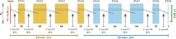
Figure 1: The architecture of the proposed CDAE that consists of a four-layer encoder and a five-layer decoder. The orange and blue boxes represent the feature vectors (FV) generated by the encoder and decoder layers, respectively. The numbers marked below the boxes are the number of filters in the corresponding convolutional layers. The batch normalization (BN) technique is applied to all layers except for the last layer.

Both the encoder and decoder parts of the proposed CDAE consist of multiple convolutional layers. We do not set a strict boundary between the two parts because we focus on the feature extraction and denoising capabilities rather than on the specific formats of the internal codes h. For the $l$-th convolutional layer that has $m_{l}$ filters, a set of $m_{l}$ feature vectors $\left(\left\{\textbf{{v}}_{i}^{(l)}\right\};i=1,2,\cdots,m_{l}\right)$ are generated as the output of this layer by convolving the output of the previous layer $\left(\left\{\textbf{{v}}_{j}^{(l-1)}\right\};j=1,2,\cdots,m_{l-1}\right)$ with each of the filters, i.e.,

$$\textbf{{v}}_{i}^{(l)}=\phi^{(l)}\left(\sum_{j=1}^{m_{l-1}}\textbf{{v}}_{j}^{(l-1)}*W_{i}^{(l)}+b_{i}^{(l)}\right),\quad i=1,2,\cdots,m_{l},$$ (1)

where $W_{i}^{(l)}$ and $b_{i}^{(l)}$ are the weights and bias of this filter in the $l$-th layer, $\phi^{(l)}(\cdot)$ is the layer’s activation function, and ‘$*$’ denotes the convolution operation.

Following the common practices (e.g., Géron, 2017; Suganuma et al., 2018), we adopt filters of size three in all layers and use the exponential linear unit (ELU; Clevert et al. 2016) as the activation function $\phi^{(l)}(\cdot)$ for all layers except the last layer, which uses the hyperbolic tangent function (i.e., tanh; see also Section 3.2). In addition, the batch normalization technique is applied to all layers except for the last layer to improve the training process as well as to act as a regularizer to prevent overfitting (Ioffe & Szegedy, 2015).

To determine the number of convolutional layers and the number of filters in each layer, we have tested multiple CDAE architectures, each containing a different number of layers and filters. After evaluating their performances (see also Section 3.3), the simplest one with sufficiently good performance is selected, which consists of a four-layer encoder with $(32,64,64,32)$ filters and a five-layer decoder with $(32,64,64,32,1)$ filters, as illustrated in Fig. 1. We note that the pooling and upsampling layers are not used in the CDAE because they have very little impact on the performance according to our tests (see also Springenberg et al., 2015).

2.3 Training and evaluation

At the beginning, the parameters of the CDAE (i.e., the weights and biases of filters in all layers) are initialized randomly using the He uniform initializer (He et al., 2015). In order to obtain an effective CDAE by training these parameters, the following three data sets are required (e.g., Ripley, 1996): (1) training set ($S_{\mathrm{tr}}$); (2) validation set ($S_{\mathrm{val}}$) that is used to validate the training process and to help determine the hyperparameters (e.g., the number of layers and filters); (3) test set ($S_{\mathrm{test}}$) that is solely used to evaluate the performance of the trained CDAE. Each data set is a collection of many data points of ($\textbf{{x}},\textbf{{x}}_{\mathrm{eor}}$), where $\textbf{{x}}=\textbf{{x}}_{\mathrm{eor}}+\textbf{{x}}_{\mathrm{fg}}$ is the total emission of one sky pixel, and $\textbf{{x}}_{\mathrm{eor}}$ is the corresponding EoR signal.

During each training epoch, the total emission $\textbf{{x}}^{(i)}$ is fed into the CDAE and goes through all the convolutional layers (Eq. 1), outputting the reconstructed EoR signal $\textbf{{r}}^{(i)}_{\mathrm{eor}}$. The difference between the reconstructed EoR signal $\textbf{{r}}^{(i)}_{\mathrm{eor}}$ and the input EoR signal $\textbf{{x}}^{(i)}_{\mathrm{eor}}$ is the loss $L$ and can be quantified with the mean squared error (MSE), i.e.,

$$L=\frac{1}{N_{\mathrm{tr}}}\sum_{i=1}^{N_{\mathrm{tr}}}\left[\textbf{{r}}_{\mathrm{eor}}^{(i)}-\textbf{{x}}_{\mathrm{eor}}^{(i)}\right]^{T}\left[\textbf{{r}}_{\mathrm{eor}}^{(i)}-\textbf{{x}}_{\mathrm{eor}}^{(i)}\right],$$ (2)

where $N_{\mathrm{tr}}$ is the number of data points in the training set $S_{\mathrm{tr}}$. By applying the back-propagation method (e.g., Rumelhart et al., 1986; LeCun et al., 1998a), the parameters are updated to reduce the loss $L$, so as to improve the quality of the reconstructed EoR signal. As the training goes for more epochs, the initially randomized CDAE is gradually shaped into a network that learns a better representation of the input and can reconstruct the EoR signal more accurately.

To evaluate the performance of the trained CDAE, the Pearson’s correlation coefficient (e.g., Harker et al., 2009; Chapman et al., 2013) is adopted to measure the similarity between the reconstructed and input EoR signals:

$$\rho(\textbf{{r}}_{\mathrm{eor}},\textbf{{x}}_{\mathrm{eor}})=\frac{\sum_{j=1}^{n}(r_{\mathrm{eor},j}-\bar{r}_{\mathrm{eor}})(x_{\mathrm{eor},j}-\bar{x}_{\mathrm{eor}})}{\sqrt{\sum_{j=1}^{n}(r_{\mathrm{eor},j}-\bar{r}_{\mathrm{eor}})^{2}\sum_{j=1}^{n}(x_{\mathrm{eor},j}-\bar{x}_{\mathrm{eor}})^{2}}},$$ (3)

where $\bar{r}_{\mathrm{eor}}$ and $\bar{x}_{\mathrm{eor}}$ represent the mean values of $\textbf{{r}}_{\mathrm{eor}}$ and $\textbf{{x}}_{\mathrm{eor}}$, respectively, and $n$ is the length of the signals. The closer to one the correlation coefficient $\rho(\textbf{{r}}_{\mathrm{eor}},\textbf{{x}}_{\mathrm{eor}})$ is, the better the achieved performance.

3 Experiments

3.1 Simulation of the SKA images

We carry out end-to-end simulations to generate the SKA images to train the proposed CDAE and evaluate its performance. A representative frequency band, namely $154162\text{\,}\mathrm{MHz}$, is chosen as an example (e.g., Datta et al., 2010) and is divided into $n_{f}=101$ channels with a resolution of $80\text{\,}\mathrm{kHz}$. At each frequency channel, the sky maps of the foreground emission and the EoR signal are simulated within an area of $10\text{\times}10\text{\,}\mathrm{\SIUnitSymbolDegree}$ and are pixelized into $1800\text{\times}1800$ with a pixel size of $20\text{\,}\mathrm{arcsec}$.

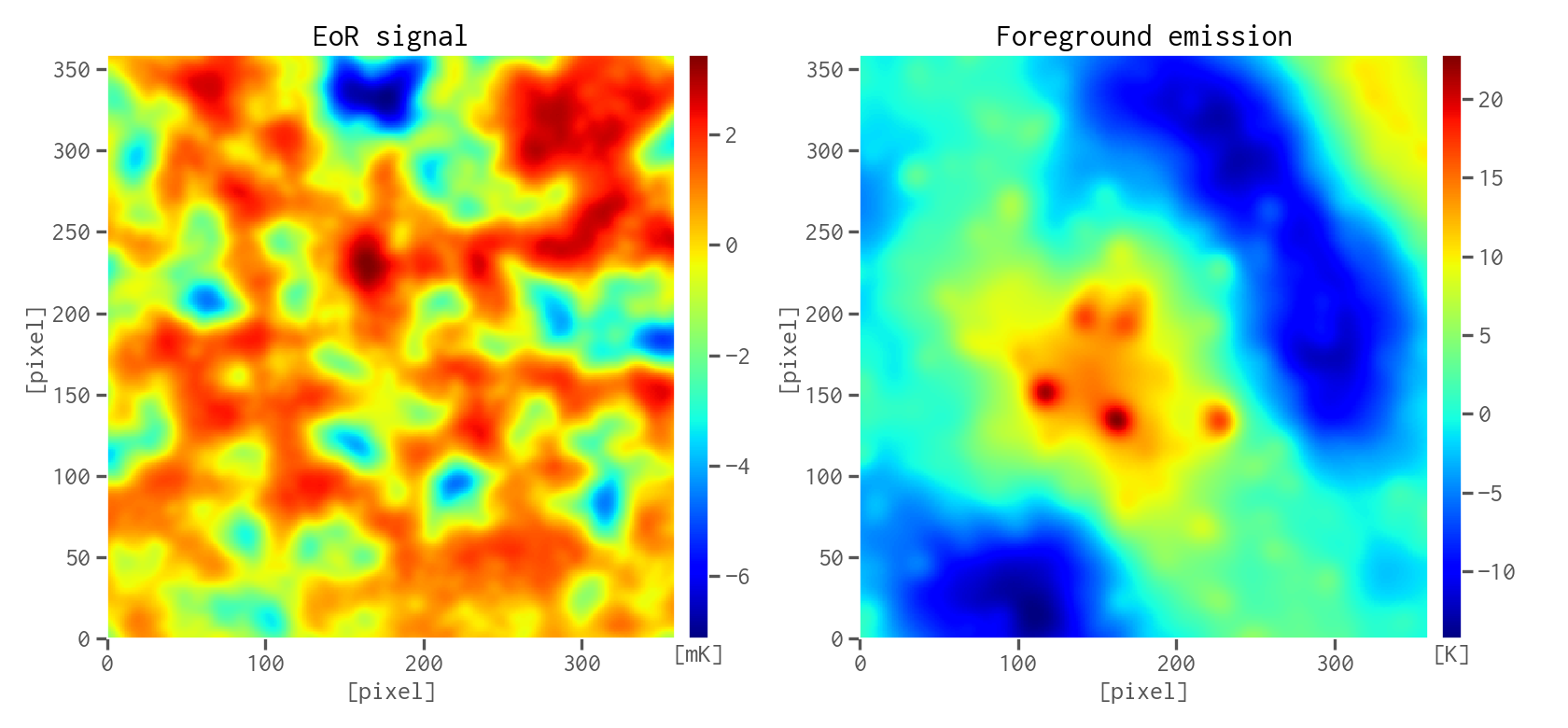
Figure 2: Simulated images of the EoR signal (left-hand panel) and the foreground emission (right-hand panel) at $158\text{\,}\mathrm{MHz}$. Both images have sizes of $360\text{\times}360$ and cover sky areas of $2\text{\times}2\text{\,}\mathrm{\SIUnitSymbolDegree}$. The blobs in the right-hand panel show the bright point sources and radio haloes.

Based on our previous work (Wang et al., 2010), we simulate the foreground emission by taking into account the contributions from the Galactic synchrotron and free-free radiations, extragalactic point sources, and radio haloes. The Galactic synchrotron radiation is simulated by extrapolating the Haslam $408\text{\,}\mathrm{MHz}$ map with a power-law spectrum, the index of which is given by the synchrotron spectral index map (Giardino et al., 2002) to account for its variation with sky positions. The reprocessed Haslam $408\text{\,}\mathrm{MHz}$ map (Remazeilles et al., 2015), which has significantly better instrument calibration and more accurate extragalactic source subtraction, is used as the template to obtain enhanced simulation results over Wang et al. (2010). By employing the tight relation between the H$\alpha$ and free-free emissions (see Dickinson et al., 2003, and references therein), the Galactic free-free radiation can be derived from the H$\alpha$ survey map (Finkbeiner, 2003). Since the Galactic diffuse emissions vary remarkably across the sky, we simulate them at a central position of (R.A., Dec.) = ($0\text{\,}\mathrm{\SIUnitSymbolDegree}$, $-27\text{\,}\mathrm{\SIUnitSymbolDegree}$), which has a high galactic latitude ($b=$-78.5\text{\,}\mathrm{\SIUnitSymbolDegree}$$) and is an appropriate choice for the simulation of SKA images (e.g., Beardsley et al., 2016). We account for the following five types of extragalactic point sources: (1) star-forming and starburst galaxies, (2) radio-quiet active galactic nuclei (AGNs), (3) Fanaroff–Riley type I and type II AGNs, (4) GHz-peaked spectrum AGNs, and (5) compact steep spectrum AGNs. The former three types of sources are simulated by utilizing the data published by Wilman et al. (2008) and the latter two types are simulated by employing their corresponding luminosity functions and spectral models. Similar to the real-time peeling of the brightest point sources in practical data analysis pipelines (e.g., Mitchell et al., 2008; Intema et al., 2009), we assume that sources with a $158\text{\,}\mathrm{MHz}$ flux density $S_{158}>$10\text{\,}\mathrm{mJy}$$ have been removed (e.g., Liu et al., 2009a). The radio haloes are simulated by generating a sample of galaxy clusters with the Press–Schechter formalism (Press & Schechter, 1974) and then applying multiple scaling relations (e.g., between cluster mass and X-ray temperature, between X-ray temperature and radio power) to derive their radio emissions.

In regard to the simulation of the EoR signal, we take advantage of the 2016 data release from the Evolution Of 21 cm Structure project (Mesinger et al., 2016) and extract the image slices at corresponding redshifts (i.e., frequencies) from the light-cone cube of the recommended ‘faint galaxies’ case. The extracted image slices are then re-scaled to match the sky coverage and pixel size of the foreground maps.

To incorporate the realistic frequency-dependent beam effects into the simulated sky maps, we further adopt the latest SKA1-Low layout configuration to simulate instrument observations. The SKA1-Low interferometer is composed of 512 stations, each of which contains 256 antennas randomly distributed inside a circle of $35\text{\,}\mathrm{m}$ in diameter. The 512 stations are divided into two parts: (1) 224 stations are randomly distributed within the ‘core’ region of $1000\text{\,}\mathrm{m}$ in diameter; (2) the remaining stations are placed on three spiral arms extending up to a radius of about $35\text{\,}\mathrm{km}$. For each sky map, we employ the OSKAR simulator (Mort et al., 2010) to perform 6-hour synthesis imaging to obtain the visibility data, from which the ‘observed’ image is created by the WSClean imager (Offringa et al., 2014). In order to emphasize the faint and relatively diffuse EoR signal, the natural weighting and baselines of $301000$ wavelengths are utilized in the imaging process. Finally, the created images are cropped to keep only the central $2\text{\times}2\text{\,}\mathrm{\SIUnitSymbolDegree}$ regions (i.e., $360\text{\times}360$ pixels) for the purpose of the best quality. Therefore, we obtain a pair of image cubes of size $360\text{\times}360\text{\times}101$ for the EoR signal $\left(C_{\mathrm{eor}}^{(1)}\right)$ and the foreground emission $\left(C_{\mathrm{fg}}^{(1)}\right)$, respectively (see Fig. 2 for the simulated images at the central frequency of $158\text{\,}\mathrm{MHz}$). To better illustrate the impacts of beam effects on the foreground spectra, we take one random sky pixel as an example and show the foreground spectra with and without the beam effects in Fig. 3, where the corresponding differential spectra (i.e., differences between every two adjacent frequency channels) and the EoR signal spectrum are also plotted. Compared to the ideal sky foreground (the top panel), the spectral smoothness of the ‘observed’ foreground (the middle panel) is seriously damaged by the rapid fluctuations resulted from the beam effects. Although such fluctuations exhibit somewhat similar spectral scales ($<$1\text{\,}\mathrm{MHz}$$) as the EoR signal (the bottom panel), they are still sufficiently different, which can be exploited by the CDAE to achieve an effective separation. We note that the ‘observed’ foreground has an amplitude of about two orders of magnitude smaller than the ideal foreground, the major reason for which is that interferometers are only sensitive to the spatial fluctuations of the emission (e.g., Braun & Walterbos, 1985).

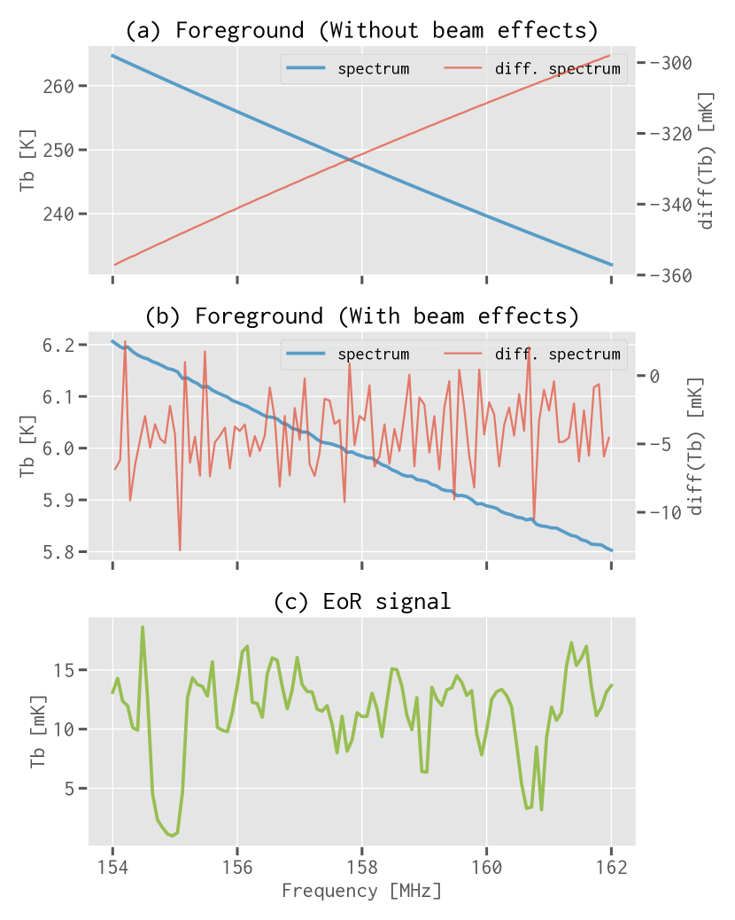
Figure 3: Example spectra of the foreground emission and the EoR signal for one random sky pixel. Top: The ideal (i.e., without beam effects) foreground spectrum (the blue line) and the corresponding differential spectrum (the red line). Middle: The ‘observed’ (i.e., with beam effects) foreground spectrum (the blue line) and the corresponding differential spectrum (the red line). Bottom: The EoR signal spectrum (the green line).

Considering that the training and evaluation of the CDAE require three data sets (i.e., training, validation, and test; Section 2.3), if there are only one pair of image cubes, the test set $S_{\mathrm{test}}$ could only contain a small fraction of all the pixels that are randomly distributed on the sky, from which it is impossible to obtain a complete image of the reconstructed EoR signal. Consequently, it is beneficial to simulate another pair of image cubes that are solely used as the test set. To this end, we simulate the Galactic diffuse radiations at a central coordinate of (R.A., Dec.) = ($3\text{\,}\mathrm{\SIUnitSymbolDegree}$, $-27\text{\,}\mathrm{\SIUnitSymbolDegree}$), i.e., $3\text{\,}\mathrm{\SIUnitSymbolDegree}$ away from the first pair of image cubes, which is sufficient because the finally cropped image cubes only cover a sky area of $2\text{\times}2\text{\,}\mathrm{\SIUnitSymbolDegree}$. Since extragalactic point sources, radio haloes, and the EoR signal are mostly isotropic, we shift their sky maps simulated above by $3\text{\,}\mathrm{\SIUnitSymbolDegree}$ to generate the new sky maps. Following the same procedures to simulate instrument observations, we obtain the second pair of image cubes $\left(C_{\mathrm{eor}}^{(2)},C_{\mathrm{fg}}^{(2)}\right)$.

We note that the simulations do not include thermal noise because the proposed method is designed to create tomographic EoR images from very deep observations that have a sufficiently low noise level. The SKA1-Low is planned to observe each of the target fields for about $1000\text{\,}\mathrm{h}$, reaching an unprecedented image noise level of $\,\lesssim$1\text{\,}\mathrm{mK}$$ that allows to directly image the reionization structures (e.g., Mellema et al., 2013; Mellema et al., 2015; Koopmans et al., 2015).

3.2 Data pre-processing

The data set $S=\{(\textbf{{x}},\,\textbf{{x}}_{\mathrm{eor}})\}$ for the CDAE is derived from the simulated image cubes $C_{\mathrm{eor}}$ and $C_{\mathrm{fg}}$, each data point $(\textbf{{x}}=\textbf{{x}}_{\mathrm{eor}}+\textbf{{x}}_{\mathrm{fg}},\,\textbf{{x}}_{\mathrm{eor}})$ representing the total emission and the EoR signal of one sky pixel, respectively. The data set thus has $N_{S}=$360\text{\times}360\text{\times}2$=$259\,200$$ data points in total.

For the input data $X=\{\textbf{{x}}\}$, we propose to apply the Fourier Transform (FT) along the frequency dimension, which makes the EoR signal more distinguishable from the foreground emission and thus easier to be learned by the CDAE (a comparison with the results derived without applying the FT is presented in Section 4.1). The Blackman–Nuttall window function is applied to suppress the FT side lobes caused by the sharp discontinuities at both ends of the finite frequency band (e.g., Chapman et al., 2016). It is sufficient to keep only half the Fourier coefficients because x is real, thus x of length $n_{f}=101$ is transformed to be 51 complex Fourier coefficients. The $n_{\mathrm{ex}}$ coefficients of the lowest Fourier frequencies are excised since they are mostly contributed by the spectral-smooth foreground emission. We adopt $n_{\mathrm{ex}}=6$ to achieve a balance between the foreground emission suppression and the EoR signal loss. The real and imaginary parts of the remaining 45 complex coefficients are then concatenated into a new real vector of length $n_{d}=90$, since the CDAE requires real data. Finally, the data are zero-centred and normalized to have unit variance.

The pre-processing steps for the input EoR signal $X_{\mathrm{eor}}=\{\textbf{{x}}_{\mathrm{eor}}\}$ are basically the same except for minor adjustments. After applying the FT, excising the $n_{\mathrm{ex}}$ lowest Fourier components, and concatenating the real and imaginary parts, the data elements that have a value less than the 1st percentile or greater than the 99th percentile are truncated, in order to prevent the possible outliers from hindering the training of the CDAE. Finally, the value range of the data is scaled to $[-1,1]$ by dividing by the maximum absolute value, which allows to use the ‘tanh’ activation function whose value range is also $[-1,1]$ in the output layer of the proposed CDAE (Section 2.2).

3.3 Training and results

The pre-processed data of the first cube pair $\left(C_{\mathrm{eor}}^{(1)},C_{\mathrm{fg}}^{(1)}\right)$ are randomly partitioned into the training set ($S_{\mathrm{tr}}$; corresponding to 80 per cent of the pixels, or $103\,680$ data points) and the validation set ($S_{\mathrm{val}}$; 20 per cent, or $25\,920$ data points). The pre-processed data of the second cube pair $\left(C_{\mathrm{eor}}^{(2)},C_{\mathrm{fg}}^{(2)}\right)$ are solely used as the test set ($S_{\mathrm{test}}$; $129\,600$ data points).

We implement the proposed CDAE using the Keras framework (Chollet et al., 2015) with the TensorFlow back end (Abadi et al., 2016), which is accelerated by the cuda toolkit. We adopt a small initial learning rate ($\alpha=${10}^{-5}$$) and use the Adam optimization method (Kingma & Ba, 2015). The CDAE is trained on the training set ($S_{\mathrm{tr}}$) with a batch size of 100 until the training loss converges, which takes about 50 epochs.

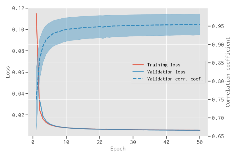
Figure 4: The training loss (the solid red line), validation loss (the solid blue line), and correlation coefficient ($\rho$; the dashed blue line with the shaded region representing its standard deviation) calculated on the validation set $S_{\mathrm{val}}$ along the training of the CDAE.

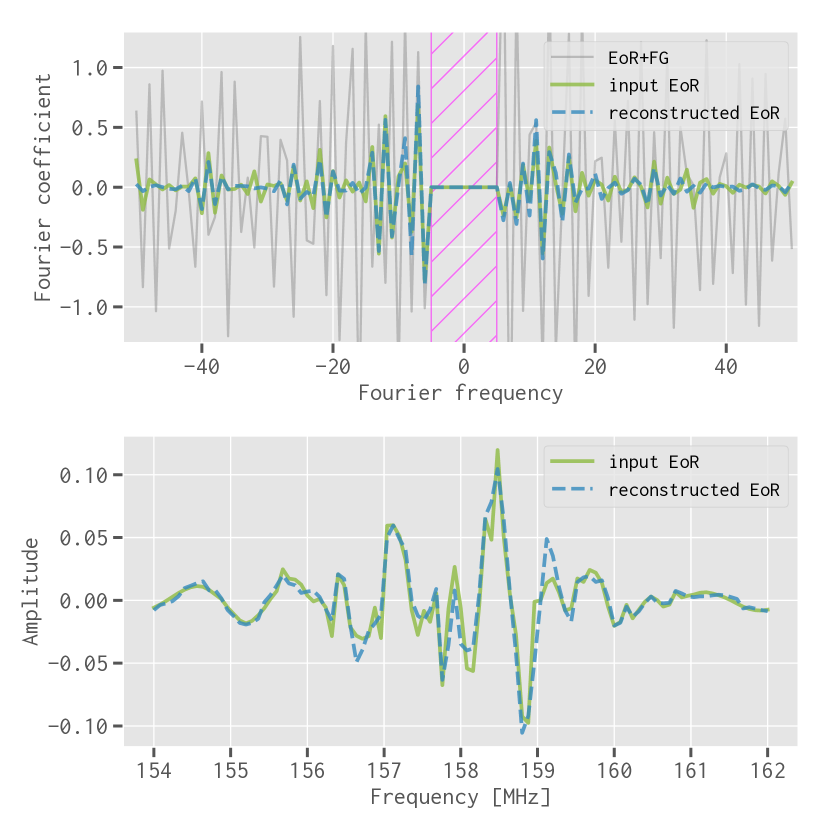
Figure 5: An example of the EoR signal reconstructed by the trained CDAE for one pixel in $S_{\mathrm{test}}$. (Top) The input EoR signal $\textbf{{x}}_{\mathrm{eor}}$ (the solid green line) and the reconstructed EoR signal $\textbf{{r}}_{\mathrm{eor}}$ (the dashed blue line) in the Fourier domain. The correlation coefficient between the input and reconstructed EoR signals is $\rho=0.931$. The grey line represents the input total emission $\textbf{{x}}=\textbf{{x}}_{\mathrm{fg}}+\textbf{{x}}_{\mathrm{eor}}$. The magenta hatched region marks the excised Fourier coefficients in data pre-processing. (Bottom) The input EoR signal $\textbf{{x}}_{\mathrm{eor}}$ (the solid green line) and the reconstructed EoR signal $\textbf{{r}}_{\mathrm{eor}}$ (the dashed blue line) transformed back to the observing frequency domain.

The training and validation losses together with the evaluation index (i.e., the correlation coefficient $\rho$) calculated on the validation set $S_{\mathrm{val}}$ during the training phase are shown in Fig. 4. The steadily decreasing losses and increasing correlation coefficient suggest that the CDAE is well trained without over-fitting. After training, the evaluation with the test set $S_{\mathrm{test}}$ yields a high correlation coefficient of $\bar{\rho}_{\mathrm{CDAE}}=$0.929\pm 0.045$$ between the reconstructed and input EoR signals. This result demonstrates that the trained CDAE achieves excellent performance in reconstructing the EoR signal. As an example, Fig. 5 illustrates the reconstructed EoR signal ($\rho=0.931$) for one pixel in $S_{\mathrm{test}}$.

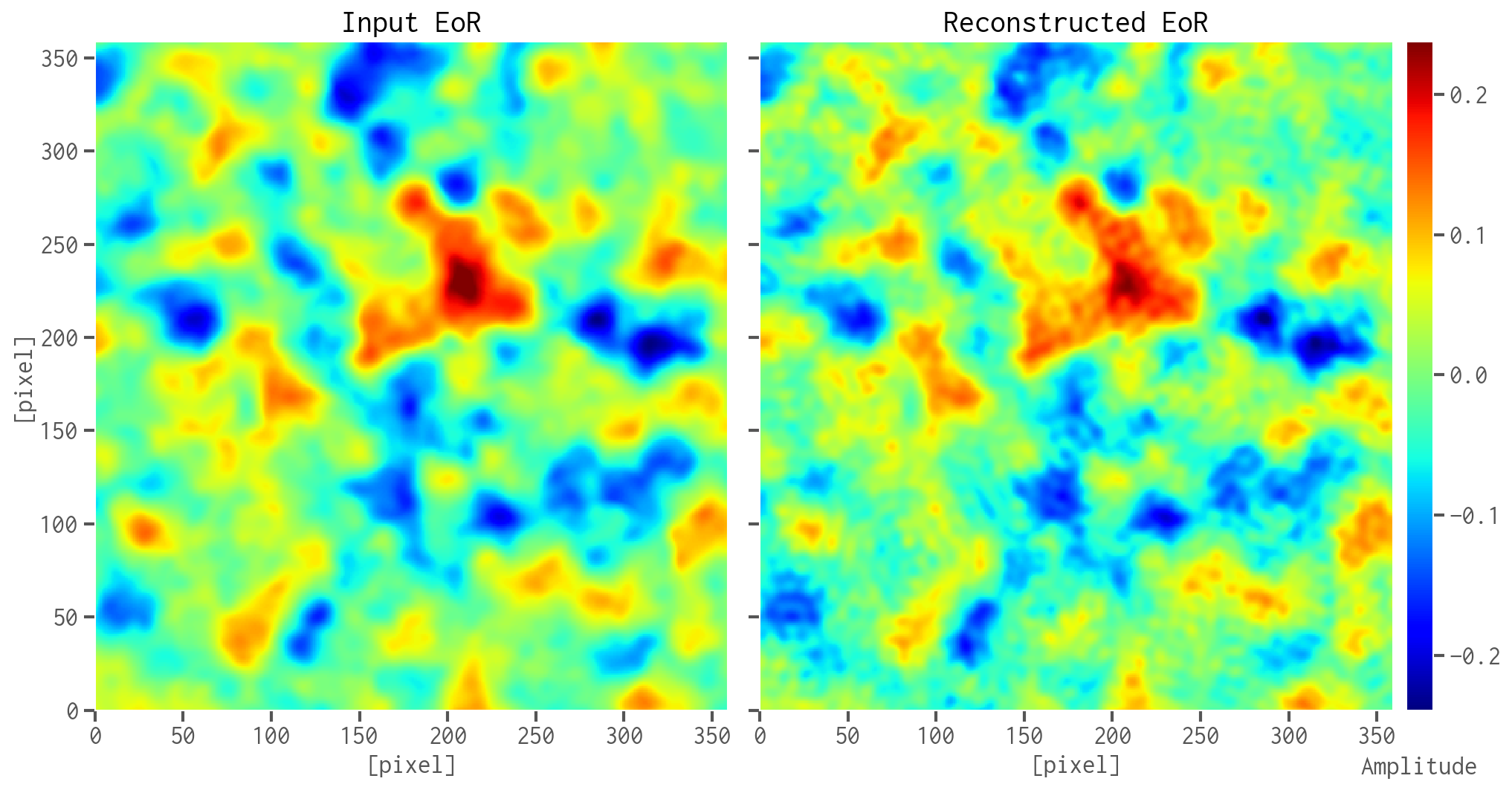
Figure 6: Comparison between the input EoR image (left-hand panel) and reconstructed EoR image (right-hand panel) at the central frequency of $158\text{\,}\mathrm{MHz}$. The images have the same size ($360\text{\times}360$ pixel) and the figures share the same colour bar (the amplitude is normalized for the CDAE).

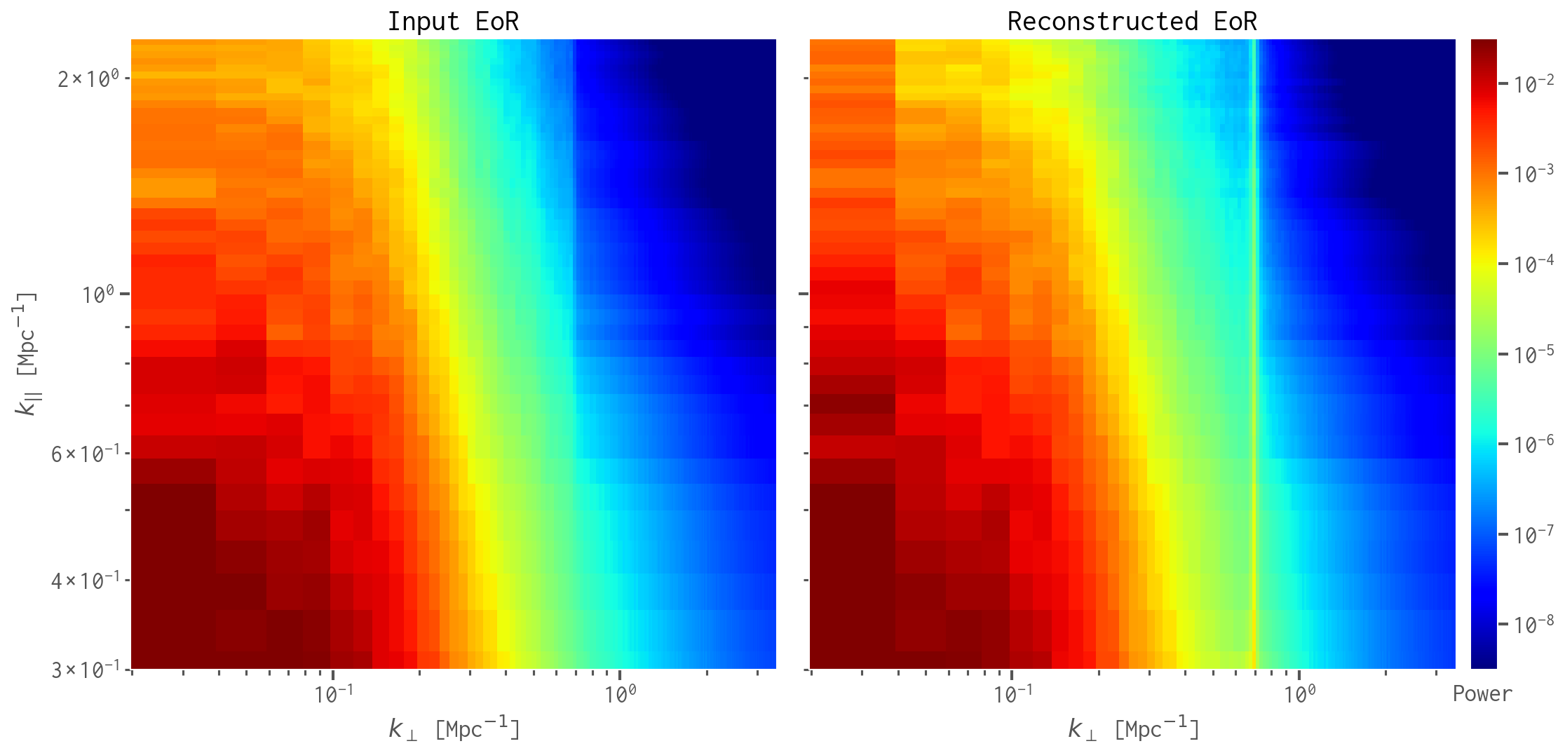
Figure 7: Comparison of two-dimensional power spectra between the input (left-hand panel) and reconstructed (right-hand panel) EoR signals.

Since the test set $S_{\mathrm{test}}$ is derived from the whole image cubes $\left(C_{\mathrm{eor}}^{(2)},C_{\mathrm{fg}}^{(2)}\right)$, we are able to create complete images of the reconstructed EoR signal and calculate the corresponding power spectrum. Taking the input and reconstructed EoR images at the central frequency of $158\text{\,}\mathrm{MHz}$ as an example (Fig. 6), the reconstructed EoR signal exhibits almost identical structures and amplitudes as the input EoR signal. We note that the reconstructed EoR image has weak but detectable redundant ripples on scales of about 10 pixels (i.e., $200\text{\,}\mathrm{arcsec}$), which are associated with the excision of the $n_{\mathrm{ex}}=6$ lowest Fourier frequencies in data pre-processing (Section 3.2). In addition, we calculate the two-dimensional power spectra from the image cubes of the input and reconstructed EoR signals (Fig. 7). It illustrates that the trained CDAE well recovers the EoR signal on all covered scales except for a very thin stripe region at $k_{\bot}\approx$0.7\text{\,}{\mathrm{Mpc}}^{-1}$$, where extra powers are generated by the aforementioned ripples in the reconstructed EoR images. We also note that there is a barely visible line at $k_{\bot}\approx$0.1\text{\,}{\mathrm{Mpc}}^{-1}$$ in both power spectra, which is caused by the boundary effect of Fourier transforming the finite frequency band.

The results clearly demonstrate that the trained CDAE is able to accurately reconstruct the EoR signal, overcoming the complicated beam effects. The achieved excellent performance of the CDAE can be mainly attributed to the architecture of stacking multiple convolutional layers, which implements a powerful feature extraction technique by hierarchically combining the basic features learned in each layer to build more and more sophisticated features (LeCun et al., 2015). Combined with the flexibility provided by the $53\,569$ trainable parameters, the CDAE, after being well trained, can intelligently learn a model that is optimised to accurately separate the faint EoR signal (e.g., Domingos, 2012).

3.4 Further validation of the CDAE

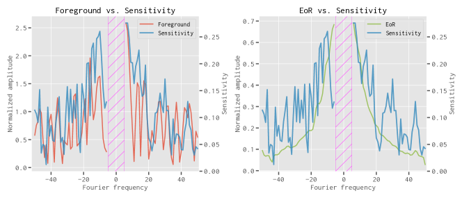
Figure 8: The CDAE’s sensitivity distribution s (blue lines in both panels) obtained by applying the occlusion method. We also plot the root-mean-square amplitudes of the foreground emission ($\textbf{{y}}_{\mathrm{fg}}$, red line in the left-hand panel) and the EoR signal ($\textbf{{y}}_{\mathrm{eor}}$, green line in the right-hand panel). The sensitivity distribution s is more correlated with the EoR signal [$\rho(\textbf{{s}},\textbf{{y}}_{\mathrm{eor}})=0.742$] than the foreground [$\rho(\textbf{{s}},\textbf{{y}}_{\mathrm{fg}})=0.562$].

With the purpose of further validating that the trained CDAE has actually learned the useful features of the EoR signal, we employ the occlusion method (Zeiler & Fergus, 2014) to visualize the sensitivity of the trained CDAE to the different part of the input data. At each time, we occlude three adjacent elements of every input x in the validation set $S_{\mathrm{val}}$, and then measure the CDAE’s sensitivity to the occluded part, which is calculated as the occlusion-induced performance loss, i.e.,

$$s=\frac{1}{N_{\mathrm{val}}}\sum_{i=1}^{N_{\mathrm{val}}}\left[\rho\left(\textbf{{r}}^{(i)}_{\mathrm{eor}},\textbf{{x}}^{(i)}_{\mathrm{eor}}\right)-\rho\left(\textbf{{R}}^{(i)}_{\mathrm{eor}},\textbf{{x}}^{(i)}_{\mathrm{eor}}\right)\right],$$ (4)

where $N_{\mathrm{val}}$ is the number of data points in the validation set, $\textbf{{x}}^{(i)}_{\mathrm{eor}}$ is the input EoR signal, and $\textbf{{r}}^{(i)}_{\mathrm{eor}}$ and $\textbf{{R}}^{(i)}_{\mathrm{eor}}$ are the reconstructed EoR signals without and with applying the occlusion, respectively. By varying the occlusion part of the input data and calculating the sensitivities, we obtain the CDAE’s sensitivity distribution (s) to every part of the input data, as shown in Fig. 8, where the root-mean-square amplitudes of the foreground emission ($\textbf{{y}}_{\mathrm{fg}}$) and the EoR signal ($\textbf{{y}}_{\mathrm{eor}}$) are also plotted. We find that the sensitivity distribution is more correlated with the EoR signal [$\rho(\textbf{{s}},\textbf{{y}}_{\mathrm{eor}})=0.742$] than the foreground [$\rho(\textbf{{s}},\textbf{{y}}_{\mathrm{fg}})=0.562$]. This verifies that the trained CDAE has learned useful features of the EoR signal to distinguish it from the foreground emission and thus becomes more sensitive to the data parts of higher signal-to-noise ratio.

4 Discussions

4.1 Why pre-process the data set with Fourier Transform?

We perform another experiment using the same CDAE architecture, data sets, and data pre-processing steps, but without applying the FT as depicted in Section 3.2. After training the CDAE in the same way as described in Section 3.3, the correlation coefficient between the reconstructed and input EoR signals evaluated on the test set $S_{\mathrm{test}}$ reaches only $\bar{\rho}_{\mathrm{noft}}=$0.628\pm 0.167$$, which indicates a significantly worse performance compared to the case with FT applied. As presented in Fig. 9, the training loss decreases more slowly and converges after about 100 epochs. We also find that the training process is slightly unstable given the small spikes on the curves of both the loss and correlation coefficient. These indicate that it is beneficial to pre-process the data set by applying the FT along the frequency dimension, because the EoR signal and the foreground emission become more distinguishable in the Fourier domain, where the fluctuating EoR signal concentrates on larger Fourier modes while the spectral-smooth foreground emission distributes mainly on smaller Fourier modes (e.g., Parsons et al., 2012).

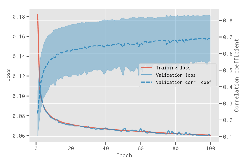
Figure 9: Same as Fig. 4 but for the case that the data are pre-processed without applying the FT.

4.2 Comparing to traditional methods

A variety of methods have been proposed to remove the foreground contamination with the aim of revealing the faint EoR signal. These methods can be broadly classified into two categories: (1) parametric methods that apply a parametric model (e.g., a low-degree polynomial) to fit and remove the foreground emission (e.g., Wang et al., 2006; Jelić et al., 2008; Liu et al., 2009b; Wang et al., 2013; Bonaldi & Brown, 2015); (2) non-parametric methods, which do not assume a specific parametric model for the foreground emission but exploit the differences between the foreground emission and the EoR signal (e.g., their different spectral features) to separate them (e.g., Harker et al., 2009; Chapman et al., 2012, 2013; Gu et al., 2013; Mertens et al., 2018).

In order to further demonstrate the performance of our method, we compare it to two representative traditional methods: the polynomial fitting method (e.g., Wang et al., 2006) and the continuous wavelet transform (CWT) method (Gu et al., 2013). The polynomial fitting method is the best representative of the parametric methods because it is widely used due to its simplicity and robustness (e.g., Jelić et al., 2008; Liu et al., 2009a; Pritchard & Loeb, 2010) and has been compared to various other foreground removal methods (e.g., Harker et al., 2009; Alonso et al., 2015; Chapman et al., 2015). Among the non-parametric category, the CWT method is chosen since it performs similarly well as other non-parametric methods, such as the Wp smoothing method (Harker et al., 2009) and the generalized morphological component analysis method (Chapman et al., 2013), meanwhile it is faster and simpler (Gu et al., 2013; Chapman et al., 2015).

With the polynomial fitting method, a low-degree polynomial is fitted along the frequency dimension for each sky pixel in the image cube of the total emission (i.e., $C_{\mathrm{tot}}=C_{\mathrm{eor}}+C_{\mathrm{fg}}$). Then by subtracting the fitted smooth component, which is regarded as the foreground emission, the EoR signal is expected to be uncovered. Using the same image cubes $\left(C_{\mathrm{eor}}^{(2)},C_{\mathrm{fg}}^{(2)}\right)$ simulated in Section 3.1, we have tested polynomials of the degree from 2 (quadratic) to 5 (quintic), and find that the quartic polynomial (degree of 4) can give the best result. However, the correlation coefficient calculated for the separated EoR signal in such a case is only $\bar{\rho}_{\mathrm{poly}}=$0.296\pm 0.121$$, which indicates that the polynomial fitting method performs poorly in removing the foreground emission.

The CWT method works based on the same assumption as other foreground removal methods that the foreground emission is spectrally smooth while the EoR signal fluctuates rapidly along the frequency dimension. After applying the CWT, the foreground emission and the EoR signal locate at different positions in the wavelet space because of their different spectral scales. Therefore, the foreground emission can be easily separated from the EoR signal and be removed (Gu et al., 2013). For each sky pixel, the spectrum of the total emission is transformed into the wavelet space by applying the CWT with the Morlet wavelet function. In the wavelet space, after identifying and removing the coefficients that are mainly contributed by the foreground emission, the remaining coefficients are transformed back to the frequency space to obtain the spectrum with the foreground emission removed, which is expected to be the EoR signal. By evaluating on the same data set $\left(C_{\mathrm{eor}}^{(2)},C_{\mathrm{fg}}^{(2)}\right)$, we have tuned the method parameters (minimum scale $s_{\mathrm{min}}$, maximum scale $s_{\mathrm{max}}$, number of scales $n_{s}$, and cone of influence $c_{i}$) and adopt $s_{\mathrm{min}}=7.4$, $s_{\mathrm{max}}=50.0$, $n_{s}=50$, and $c_{i}=1.6$ to obtain the relatively best performance, which is, however, only $\bar{\rho}_{\mathrm{cwt}}=$0.198\pm 0.160$$. We note that the CWT method performs slightly worse than the polynomial fitting method, which is different from the comparison in Gu et al. (2013). This may be caused by the more serious boundary effect since our simulated data have a narrower bandwidth and coarser frequency resolution than those of Gu et al. (2013).

The main reason that both traditional foreground removal methods only obtain remarkably inferior results is that the smoothness of the foreground spectra is seriously damaged by the frequency-dependent beam effects, which cause rapid fluctuations of strength the same order as the EoR signal on the originally smooth foreground spectra (Fig. 3b). As a result, the foreground spectra complicated by the beam effects cannot be well fitted by a low-degree polynomial and have more similar spectral scales as the EoR signal. In consequence, both methods are unable to well model the complicated foreground spectra and thus have great difficulties in removing them. On the contrary, given its data-driven nature and powerful feature extraction capabilities, the CDAE is able to distil knowledge from the training data and learns the features to distinguish the EoR signal from the fluctuations arising from the beam effects. Hence, the CDAE achieves superior performance in separating the EoR signal.

5 Summary

The frequency-dependent beam effects of interferometers can cause rapid fluctuations along the frequency dimension, which damage the smoothness of the foreground spectra and prevent traditional foreground removal methods from uncovering the EoR signal. Given the difficulties in crafting practicable models to overcome the complicated beam effects, methods that can intelligently learn tailored models from the data seem more feasible and appealing. To this end, we have proposed a deep-learning-based method that uses a nine-layer CDAE to separate the EoR signal. The CDAE has been trained on the simulated SKA images and has achieved excellent performance. We conclude that the CDAE has outstanding ability to overcome the complicated beam effects and accurately separate the faint EoR signal, exhibiting the great potential of deep-learning-based methods to play an important role in the forthcoming EoR experiments.

References

- Abadi et al. (2016) Abadi M., et al., 2016, in Proceedings of 12th USENIX Symposium on Operating Systems Design and Implementation (OSDI 2016). USENIX Association, https://www.tensorflow.org/
- Alonso et al. (2015) Alonso D., Bull P., Ferreira P. G., Santos M. G., 2015, MNRAS, 447, 400
- Beardsley et al. (2016) Beardsley A. P., et al., 2016, ApJ, 833, 102
- Bengio et al. (2013) Bengio Y., Yao L., Alain G., Vincent P., 2013, in Proceedings of the 26th International Conference on Neural Information Processing Systems (NIPS 2013). Curran Associates Inc., USA, pp 899–907, http://dl.acm.org/citation.cfm?id=2999611.2999712
- Bonaldi & Brown (2015) Bonaldi A., Brown M. L., 2015, MNRAS, 447, 1973
- Braun & Walterbos (1985) Braun R., Walterbos R. A. M., 1985, A&A, 143, 307
- Chapman et al. (2012) Chapman E., et al., 2012, MNRAS, 423, 2518
- Chapman et al. (2013) Chapman E., et al., 2013, MNRAS, 429, 165
- Chapman et al. (2015) Chapman E., et al., 2015, Advancing Astrophysics with the Square Kilometre Array (AASKA14), p. 5
- Chapman et al. (2016) Chapman E., Zaroubi S., Abdalla F. B., Dulwich F., Jelić V., Mort B., 2016, MNRAS, 458, 2928
- Chollet et al. (2015) Chollet F., et al., 2015, Keras, https://keras.io
- Clevert et al. (2016) Clevert D.-A., Unterthiner T., Hochreiter S., 2016, in The International Conference on Learning Representations (ICLR 2016). (arXiv:1511.07289)
- Datta et al. (2010) Datta A., Bowman J. D., Carilli C. L., 2010, ApJ, 724, 526
- Dickinson et al. (2003) Dickinson C., Davies R. D., Davis R. J., 2003, MNRAS, 341, 369
- Domingos (2012) Domingos P., 2012, Communications of the ACM, 55, 78
- Du et al. (2017) Du B., Xiong W., Wu J., Zhang L., Zhang L., Tao D., 2017, IEEE Transactions on Cybernetics, 47, 1017
- Finkbeiner (2003) Finkbeiner D. P., 2003, ApJS, 146, 407
- Furlanetto (2016) Furlanetto S. R., 2016, Understanding the Epoch of Cosmic Reionization: Challenges and Progress, 423, 247
- Géron (2017) Géron A., 2017, Hands-On Machine Learning with Scikit-Learn and TensorFlow: Concepts, Tools, and Techniques to Build Intelligent Systems, 1st edn. O’Reilly Media, Inc.
- Giardino et al. (2002) Giardino G., Banday A. J., Górski K. M., Bennett K., Jonas J. L., Tauber J., 2002, A&A, 387, 82
- Goodfellow et al. (2016) Goodfellow I., Bengio Y., Courville A., 2016, Deep Learning. MIT Press, http://www.deeplearningbook.org
- Grais & Plumbley (2017) Grais E. M., Plumbley M. D., 2017, in 5th IEEE Global Conference on Signal and Information Processing (GlobalSIP 2017). IEEE, pp 1265–1269 (arXiv:1703.08019), doi:10.1109/GlobalSIP.2017.8309164
- Gu et al. (2013) Gu J., Xu H., Wang J., An T., Chen W., 2013, ApJ, 773, 38
- Harker et al. (2009) Harker G., et al., 2009, MNRAS, 397, 1138
- He et al. (2015) He K., Zhang X., Ren S., Sun J., 2015, in Proceedings of the 2015 IEEE International Conference on Computer Vision (ICCV 2015). IEEE Computer Society, Washington DC, USA, pp 1026–1034, doi:10.1109/ICCV.2015.123
- Herbel et al. (2018) Herbel J., Kacprzak T., Amara A., Refregier A., Lucchi A., 2018, Journal of Cosmology and Astro-Particle Physics, 2018, 054
- Hinton & Salakhutdinov (2006) Hinton G. E., Salakhutdinov R. R., 2006, Science, 313, 504
- Intema et al. (2009) Intema H. T., van der Tol S., Cotton W. D., Cohen A. S., van Bemmel I. M., Röttgering H. J. A., 2009, A&A, 501, 1185
- Ioffe & Szegedy (2015) Ioffe S., Szegedy C., 2015, in Proceedings of the 32nd International Conference on International Conference on Machine Learning (ICML 2015). PMLR, pp 448–456
- Jelić et al. (2008) Jelić V., et al., 2008, MNRAS, 389, 1319
- Kingma & Ba (2015) Kingma D. P., Ba J., 2015, in International Conference on Learning Representations (ICLR 2015). (arXiv:1412.6980)
- Koopmans et al. (2015) Koopmans L., et al., 2015, Advancing Astrophysics with the Square Kilometre Array (AASKA14), p. 1
- Krizhevsky et al. (2012) Krizhevsky A., Sutskever I., Hinton G. E., 2012, in Proceedings of the 25th International Conference on Neural Information Processing Systems (NIPS). Curran Associates Inc., USA, pp 1097–1105, http://dl.acm.org/citation.cfm?id=2999134.2999257
- LeCun et al. (1998a) LeCun Y., Bottou L., Orr G. B., Müller K.-R., 1998a, in Neural Networks: Tricks of the Trade. Springer-Verlag, London, UK, UK, pp 9–50, http://dl.acm.org/citation.cfm?id=645754.668382
- LeCun et al. (1998b) LeCun Y., Bottou L., Bengio Y., Haffner P., 1998b, Proceedings of the IEEE, 86, 2278
- LeCun et al. (2015) LeCun Y., Bengio Y., Hinton G., 2015, Nature, 521, 436
- Liu et al. (2009a) Liu A., Tegmark M., Zaldarriaga M., 2009a, MNRAS, 394, 1575
- Liu et al. (2009b) Liu A., Tegmark M., Bowman J., Hewitt J., Zaldarriaga M., 2009b, MNRAS, 398, 401
- Lochner et al. (2015) Lochner M., Natarajan I., Zwart J. T. L., Smirnov O., Bassett B. A., Oozeer N., Kunz M., 2015, MNRAS, 450, 1308
- Lu et al. (2013) Lu X., Tsao Y., Matsuda S., Hori C., 2013, in 14th Annual Conference of the International Speech Communication Association (INTERSPEECH 2013). pp 436–440, https://www.isca-speech.org/archive/interspeech_2013/i13_0436.html
- Ma et al. (2019) Ma Z., et al., 2019, ApJS, 240, 34
- Masci et al. (2011) Masci J., Meier U., Cireşan D., Schmidhuber J., 2011, in Proceedings of the 21th International Conference on Artificial Neural Networks (ICANN 2011). Springer-Verlag, pp 52–59, http://dl.acm.org/citation.cfm?id=2029556.2029563
- Mellema et al. (2013) Mellema G., et al., 2013, Experimental Astronomy, 36, 235
- Mellema et al. (2015) Mellema G., Koopmans L., Shukla H., Datta K. K., Mesinger A., Majumdar S., 2015, Advancing Astrophysics with the Square Kilometre Array (AASKA14), p. 10
- Mertens et al. (2018) Mertens F. G., Ghosh A., Koopmans L. V. E., 2018, MNRAS, 478, 3640
- Mesinger et al. (2016) Mesinger A., Greig B., Sobacchi E., 2016, MNRAS, 459, 2342
- Mitchell et al. (2008) Mitchell D. A., Greenhill L. J., Wayth R. B., Sault R. J., Lonsdale C. J., Cappallo R. J., Morales M. F., Ord S. M., 2008, IEEE Journal of Selected Topics in Signal Processing, 2, 707
- Morales & Wyithe (2010) Morales M. F., Wyithe J. S. B., 2010, ARA&A, 48, 127
- Mort et al. (2010) Mort B. J., Dulwich F., Salvini S., Adami K. Z., Jones M. E., 2010, in IEEE International Symposium on Phased Array Systems and Technology. IEEE, pp 690–694, doi:10.1109/ARRAY.2010.5613289
- Offringa et al. (2014) Offringa A. R., et al., 2014, MNRAS, 444, 606
- Parsons et al. (2012) Parsons A. R., Pober J. C., Aguirre J. E., Carilli C. L., Jacobs D. C., Moore D. F., 2012, ApJ, 756, 165
- Press & Schechter (1974) Press W. H., Schechter P., 1974, ApJ, 187, 425
- Pritchard & Loeb (2010) Pritchard J. R., Loeb A., 2010, Phys. Rev. D, 82, 023006
- Remazeilles et al. (2015) Remazeilles M., Dickinson C., Banday A. J., Bigot-Sazy M.-A., Ghosh T., 2015, MNRAS, 451, 4311
- Ripley (1996) Ripley B. D., 1996, Pattern Recognition and Neural Networks. Cambridge University Press, doi:10.1017/CBO9780511812651
- Rumelhart et al. (1986) Rumelhart D. E., Hinton G. E., Williams R. J., 1986, Nature, 323, 533
- Shen et al. (2017) Shen H., George D., Huerta E. A., Zhao Z., 2017, preprint, (arXiv:1711.09919)
- Simonyan & Zisserman (2014) Simonyan K., Zisserman A., 2014, preprint, (arXiv:1409.1556)
- Springenberg et al. (2015) Springenberg J. T., Dosovitskiy A., Brox T., Riedmiller M., 2015, in International Conference on Learning Representations (ICLR 2015). (arXiv:1412.6806)
- Suganuma et al. (2018) Suganuma M., Ozay M., Okatani T., 2018, in Proceedings of the 35th International Conference on Machine Learning (ICML 2018). PMLR, p. 4771 (arXiv:1803.00370)
- Szegedy et al. (2015) Szegedy C., et al., 2015, in IEEE Conference on Computer Vision and Pattern Recognition (CVPR 2015). IEEE, pp 1–9 (arXiv:1409.4842), doi:10.1109/CVPR.2015.7298594
- Vafaei Sadr et al. (2019) Vafaei Sadr A., Vos E. E., Bassett B. A., Hosenie Z., Oozeer N., Lochner M., 2019, MNRAS, 484, 2793
- Vincent et al. (2008) Vincent P., Larochelle H., Bengio Y., Manzagol P.-A., 2008, in Proceedings of the 25th International Conference on Machine Learning (ICML 2008). ACM, pp 1096–1103, doi:10.1145/1390156.1390294
- Vincent et al. (2010) Vincent P., Larochelle H., Lajoie I., Bengio Y., Manzagol P.-A., 2010, The Journal of Machine Learning Research, 11, 3371
- Wang et al. (2006) Wang X., Tegmark M., Santos M. G., Knox L., 2006, ApJ, 650, 529
- Wang et al. (2010) Wang J., et al., 2010, ApJ, 723, 620
- Wang et al. (2013) Wang J., et al., 2013, ApJ, 763, 90
- Wang et al. (2014) Wang W., Huang Y., Wang Y., Wang L., 2014, in IEEE Conference on Computer Vision and Pattern Recognition Workshops. IEEE, pp 496–503, doi:10.1109/CVPRW.2014.79
- Wilman et al. (2008) Wilman R. J., et al., 2008, MNRAS, 388, 1335
- Xie et al. (2012) Xie J., Xu L., Chen E., 2012, in Proceedings of the 25th International Conference on Neural Information Processing Systems (NIPS 2012). Curran Associates Inc., USA, pp 341–349
- Zeiler & Fergus (2014) Zeiler M. D., Fergus R., 2014, in Fleet D., Pajdla T., Schiele B., Tuytelaars T., eds, European Conference on Computer Vision (ECCV 2014). Springer-Verlag, pp 818–833 (arXiv:1311.2901), doi:10.1007/978-3-319-10590-1_53