Nonlinear Approximation via Compositions

Abstract

Given a function dictionary $\mathcal{D}$ and an approximation budget $N\in\mathbb{N}^{+}$, nonlinear approximation seeks the linear combination of the best $N$ terms $\{T_{n}\}_{1\leq n\leq N}\subseteq\mathcal{D}$ to approximate a given function $f$ with the minimum approximation error

$$\varepsilon_{L,f}:=\min_{\{g_{n}\}\subseteq{\mathbb{R}},\{T_{n}\}\subseteq\mathcal{D}}\|f(\bm{x})-\sum_{n=1}^{N}g_{n}T_{n}(\bm{x})\|.$$

Motivated by recent success of deep learning, we propose dictionaries with functions in a form of compositions, i.e.,

$$T(\bm{x})=T^{(L)}\circ T^{(L-1)}\circ\cdots\circ T^{(1)}(\bm{x})$$

for all $T\in\mathcal{D}$, and implement $T$ using ReLU feed-forward neural networks (FNNs) with $L$ hidden layers. We further quantify the improvement of the best $N$-term approximation rate in terms of $N$ when $L$ is increased from $1$ to $2$ or $3$ to show the power of compositions. In the case when $L>3$, our analysis shows that increasing $L$ cannot improve the approximation rate in terms of $N$.

In particular, for any function $f$ on $[0,1]$, regardless of its smoothness and even the continuity, if $f$ can be approximated using a dictionary when $L=1$ with the best $N$-term approximation rate $\varepsilon_{L,f}=\mathcal{O}(N^{-\eta})$, we show that dictionaries with $L=2$ can improve the best $N$-term approximation rate to $\varepsilon_{L,f}=\mathcal{O}(N^{-2\eta})$. We also show that for Hölder continuous functions of order $\alpha$ on $[0,1]^{d}$, the application of a dictionary with $L=3$ in nonlinear approximation can achieve an essentially tight best $N$-term approximation rate $\varepsilon_{L,f}=\mathcal{O}(N^{-2\alpha/d})$. Finally, we show that dictionaries consisting of wide FNNs with a few hidden layers are more attractive in terms of computational efficiency than dictionaries with narrow and very deep FNNs for approximating Hölder continuous functions if the number of computer cores is larger than $N$ in parallel computing.

1 Introduction

For non-smooth and high-dimensional function approximation, a favorable technique popularized in recent decades is the nonlinear approximation devore_1998 that does not limit the approximants to come from linear spaces, obtaining sparser representation, cheaper computation, and more robust estimation, and therein emerged the bloom of many breakthroughs in applied mathematics and computer science (e.g., wavelet analysis doi:10.1137/1.9781611970104, dictionary learning DBLP:journals/corr/TariyalMSV16, data compression and denoising 600614; 374249, adaptive pursuit Davis94adaptivenonlinear; 6810285, compressed sensing 1614066; 4472240).

Typically, nonlinear approximation is a two-stage algorithm that designs a good redundant nonlinear dictionary, $\mathcal{D}$, in its first stage, and identifies the optimal approximant as a linear combination of $N$ elements of $\mathcal{D}$ in the second stage:

$$f(\bm{x})\approx g\circ T(\bm{x}):=\sum_{n=1}^{N}g_{n}T_{n}(\bm{x}),$$ (1.1)

where $f(\bm{x})$ is the target function in a Hilbert space $\mathcal{H}$ associated with a norm denoted as $\|\cdot\|_{*}$, $\{T_{n}\}\subseteq\mathcal{D}\subseteq\mathcal{H}$, $T$ is a nonlinear map from $\mathbb{R}^{d}$ to $\mathbb{R}^{N}$ with the $n$-th coordinate being $T_{n}$, and $g$ is a linear map from $\mathbb{R}^{N}$ to $\mathbb{R}$ with the $n$-th coordinate being $g_{n}\in\mathbb{R}$. The nonlinear approximation seeks $g$ and $T$ such that

$$\{\{T_{n}\},\{g_{n}\}\}=\operatorname*{arg\,min}_{\{g_{n}\}\subseteq{\mathbb{R}},\{T_{n}\}\subseteq\mathcal{D}}\|f(\bm{x})-\sum_{n=1}^{N}g_{n}T_{n}(\bm{x})\|_{*},$$ (1.2)

which is also called the best $N$-term approximation. One remarkable approach of nonlinear approximation is based on one-hidden-layer neural networks that give simple and elegant bases of the form $T(\bm{x})=\sigma(\bm{W}\bm{x}+\bm{b})$, where $\bm{W}\bm{x}+\bm{b}$ is a linear transform in $\bm{x}$ with the transformation matrix $\bm{W}$ (named as the weight matrix) and a shifting vector $\bm{b}$ (called bias), and $\sigma$ is a nonlinear function (called the activation function). The approximation

$$f(\bm{x})\approx\sum_{n=1}^{N}g_{n}T_{n}(\bm{x})=\sum_{n=1}^{N}g_{n}\sigma(\bm{W}_{n}\bm{x}+\bm{b}_{n})$$

includes wavelets pursuits 258082; 471413, adaptive splines devore_1998; PETRUSHEV2003158, radial basis functions radiusbase; HANGELBROEK2010203; Xie2013, sigmoidal neural networks Sig1; Sig2; Sig3; Sig4; Sig5; Cybenko1989ApproximationBS; HORNIK1989359; barron1993, etc. For functions in Besov spaces with smoothness $s$, radiusbase; HANGELBROEK2010203 constructed an $\mathcal{O}(N^{-s/d})$ approximation that is almost optimal Lin2014 and the smoothness cannot be reduced generally HANGELBROEK2010203. For Hölder continuous functions of order $1$ on $[0,1]^{d}$, Xie2013 essentially constructed an $\mathcal{O}(N^{-\frac{1}{2d}})$ approximation, which is far from the lower bound $\mathcal{O}(N^{-2/d})$ as we shall prove in this paper. Achieving the optimal approximation rate of general continuous functions in constructive approximation, especially in high dimensional spaces, remains an unsolved challenging problem.

1.1 Problem Statement

ReLU FNNs have been proved to be a powerful tool in many fields from various points of view NIPS2014_5422; 6697897; Bartlett98almostlinear; Sakurai; pmlr-v65-harvey17a; Kearns; Anthony:2009; PETERSEN2018296, which motivates us to tackle the open problem above via function compositions in the nonlinear approximation using deep ReLU FNNs, i.e.,

$$f(\bm{x})\approx g\circ T^{(L)}\circ T^{(L-1)}\circ\cdots\circ T^{(1)}(\bm{x}),$$ (1.3)

where $T^{(i)}(\bm{x})=\sigma\left(\bm{W}_{i}\bm{x}+\bm{b}_{i}\right)$ with $\bm{W}_{i}\in\mathbb{R}^{N_{i}\times N_{i-1}}$, $\bm{b}_{i}\in\mathbb{R}^{N_{i}}$ for $i=1,\dots,L$, $\sigma$ is the ReLU activation function, and $f$ is a Hölder continuous function. For the convenience of analysis, we consider $N_{i}=N$ for $i=1,\dots,L$. Let $\mathcal{D}_{L}$ be the dictionary consisting of ReLU FNNs $g\circ T^{(L)}\circ T^{(L-1)}\circ\cdots\circ T^{(1)}(\bm{x})$ with width $N$ and depth $L$. To identify the optimal FNN to approximate $f(\bm{x})$, it is sufficient to solve the following optimization problem

$$\phi^{*}=\operatorname*{arg\,min}_{\phi\in\mathcal{D}_{L}}\|f-\phi\|_{*}.$$ (1.4)

The fundamental limit of nonlinear approximation via the proposed dictionary is essentially determined by the approximation power of function compositions in (1.3), which gives a performance guarantee of the minimizer in (1.4). Since function compositions are implemented via ReLU FNNs, the remaining problem is to quantify the approximation capacity of deep ReLU FNNs, especially their ability to improve the best $N$-term approximation rate in $N$ for any fixed $L$ defined as

$$\varepsilon_{L,f}(N)=\min_{\phi\in\mathcal{D}_{L}}\|f-\phi\|_{*}.$$ (1.5)

Function compositions can significantly enrich the dictionary of nonlinear approximation and this idea was not considered in the literature previously due to the expensive computation of function compositions in solving the minimization problem in (1.4). Fortunately, recent development of efficient algorithms for optimization with compositions (e.g., backpropagation techniques werbos1975beyond; Fukushima1980; rumelhart1986psychological and parallel computing techniques 10.1007/978-3-642-15825-4_10; Ciresan:2011:FHP:2283516.2283603) makes it possible to explore the proposed dictionary in this paper. Furthermore, with advanced optimization algorithms Duchi:2011:ASM:1953048.2021068; Johnson:2013:ASG:2999611.2999647; ADAM, good local minima of (1.4) can be identified efficiently NIPS2016_6112; DBLP:journals/corr/NguyenH17; opt.

1.2 Related work and contribution

The main goal in the remaining article is to quantify the best $N$-term approximation rate $\varepsilon_{L,f}(N)$ defined in (1.5) for ReLU FNNs in the dictionary $\mathcal{D}_{L}$ with a fixed depth $L$ when $f$ is a Hölder continuous function. This topic is related to several existing approximation theories in the literature, but none of these existing works can be applied to answer the problem addressed in this paper.

First of all, this paper identifies explicit formulas for the best $N$-term approximation rate

$$\varepsilon_{L,f}(N)\leq\begin{cases}2\nu N^{-2\alpha},&\text{when $L\geq 2$ and $d=1$,}\\ 2(2\sqrt{d})^{\alpha}\nu N^{-2\alpha/d},&\text{when $L\geq 3$ and $d>1$},\end{cases}$$ (1.6)

for any $N\in\mathbb{N}^{+}$ and a Hölder continuous function $f$ of order $\alpha$ with a constant $\nu$, while existing theories NIPS2017_7203; bandlimit; yarotsky2017; DBLP:journals/corr/LiangS16; Hadrien; suzuki2018adaptivity; PETERSEN2018296; yarotsky18a; DBLP:journals/corr/abs-1807-00297 can only provide implicit formulas in the sense that the approximation error contains an unknown prefactor and work only for sufficiently large $N$ or $L$ larger than some unknown numbers. For example, the approximation rate in yarotsky18a via a narrow and deep ReLU FNN is $c(d)L^{-2\alpha/d}$ with $c(d)$ unknown and for $L$ larger than a sufficiently large unknown number $\mathcal{L}$; the approximation rate in yarotsky18a via a wide and shallow ($c_{1}(d)$-layer) ReLU FNN is $c_{2}(d)N^{-\alpha/d}$ with $c_{1}(d)$ and $c_{2}(d)$ unknown and for $N$ larger than a sufficiently large unknown number $\mathcal{N}$. For another example, given an approximation error $\varepsilon$, PETERSEN2018296 proved the existence of a ReLU FNN with a constant but still unknown number of layers approximating a $C^{\beta}$ function within the target error. Similarly, given the $\varepsilon$ error, Hadrien; bandlimit; DBLP:journals/corr/abs-1807-00297 estimate the scaling of the network size in $\varepsilon$ and the scaling contains unknown prefactors. Given an arbitrary $L$ and $N$, no existing work can provide an explicit formula for the approximation error to guide practical network design, e.g., to guarantee whether the network is large enough to meet the accuracy requirement. This paper provides such formulas for the first time and in fact the bound in these formulas is asymptotically tight as we shall prove later.

Second, our target functions are Hölder continuous, while most of existing works aim for a smaller function space with certain smoothness, e.g. functions in $C^{\alpha}([0,1]^{d})$ with $\alpha\geq 1$ NIPS2017_7203; DBLP:journals/corr/LiangS16; yarotsky2017; DBLP:journals/corr/abs-1807-00297, band-limited functions bandlimit, Korobov spaces Hadrien, or Besev spaces suzuki2018adaptivity. To the best of our knowledge, there is only one existing article yarotsky18a concerning the approximation power of deep ReLU FNNs for $C([0,1]^{d})$. However, the conclusion of yarotsky18a only works for ReLU FNNs with a fixed width $2d+10$ and a sufficiently large $L$, instead of a fixed $L$ and an arbitrary $N$ as required in the nonlinear approximation (see Figure 1 for the comparison of the conclusion of yarotsky18a and this paper).

As we can see in Figure 1, the improvement of the best $N$-term approximation rate in terms of $N$ when $L$ is increased from $1$ to $2$ or $3$ is significant, which shows the power of depth in ReLU FNNs. However, in the case when $L>3$, our analysis shows that increasing $L$ cannot improve the approximation rate in terms of $N$. As an interesting corollary of our analysis, for any function $f$ on $[0,1]$, regardless of its smoothness and even the continuity, if $f$ can be approximated using using functions in $\mathcal{D}_{1}$ with the best $N$-term approximation rate $\varepsilon_{L,f}=\mathcal{O}(N^{-\eta})$, we show that functions in $\mathcal{D}_{2}$ can improve the best $N$-term approximation rate to $\varepsilon_{L,f}=\mathcal{O}(N^{-2\eta})$. Extending this conclusion for a general $d$ dimensional function is challenging and we leave it as future work.

From the point of view of analysis techniques, this paper introduce new analysis methods merely based on the structure of FNNs, while existing works NIPS2017_7203; bandlimit; yarotsky2017; DBLP:journals/corr/LiangS16; Hadrien; suzuki2018adaptivity; PETERSEN2018296; yarotsky18a; DBLP:journals/corr/abs-1807-00297 rely on constructing FNNs to approximate traditional basis in approximation theory, e.g., polynomials, splines, and sparse grids, which are used to approximate smooth functions.

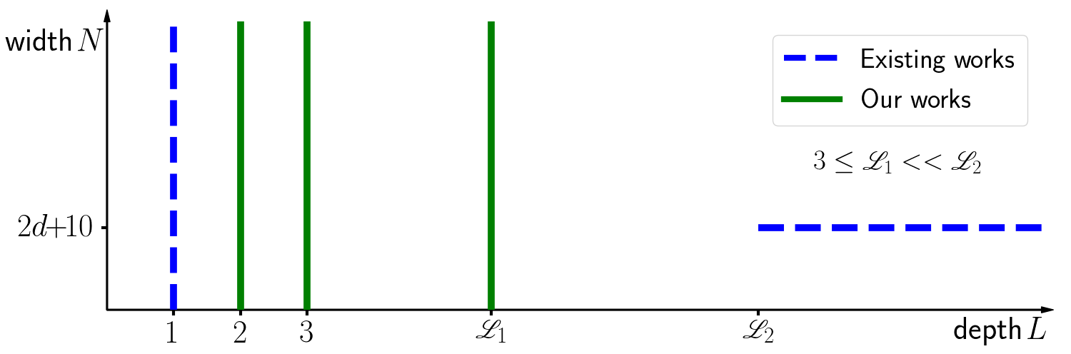
Figure 1: A comparison of existing works and our contribution on the approximation power of ReLU FNNs for Hölder continuous functions of order $\alpha$. Existing results in two cases: 1) $\mathcal{O}(N^{-\alpha/d})$ approximation rate for ReLU FNNs with depth $L=1$ and width $N$; 2) $\mathcal{O}(L^{-2\alpha/d})$ approximation rate for ReLU FNNs with depth $L$ larger than a sufficiently large unknown number $\mathscr{L}_{2}$ and width $2d+10$. Our contribution: $\mathcal{O}(N^{-2\alpha/d})$ approximation rate for ReLU FNNs width depth $L\geq 3$ and width $N$ in the case of $d>1$ ($L\geq 2$ in the case of $d=1$).

Finally, we analyze the approximation efficiency of neural networks in parallel computing, a very important point of view that was not paid attention to in the literature. In most applications, the efficiency of deep learning computation highly relies on parallel computation. We show that a narrow and very deep neural network is inefficient if its approximation rate is not exponentially better than wide and shallower networks. Hence, neural networks with $\mathcal{O}(1)$ layers are more attractive in modern computational platforms, considering the computational efficiency per training iteration in parallel computing platforms. Our conclusion does not conflict with the current state-of-the-art deep learning research since most of these successful deep neural networks have a depth that is asymptotically $\mathcal{O}(1)$ relative to the width.

1.3 Organization

The rest of the paper is organized as follows. Section 2 summarizes the notations throughout this paper. Section 3 presents the main theorems while Section LABEL:sec:numerical shows numerical tests in parallel computing to support the claims in this paper. Finally, Section LABEL:sec:con concludes this paper with a short discussion.

2 Preliminaries

For the purpose of convenience, we present notations and elementary lemmas used throughout this paper as follows.

2.1 Notations

• Matrices are denoted by bold uppercase letters, e.g., $\bm{A}\in\mathbb{R}^{m\times n}$ is a real matrix of size $m\times n$, and $\bm{A}^{T}$ denotes the transpose of $\bm{A}$. Correspondingly, $\bm{A}(i,j)$ is the $(i,j)$-th entry of $\bm{A}$; $\bm{A}(:,j)$ is the $j$-th column of $\bm{A}$; $\bm{A}(i,:)$ is the $i$-th row of $\bm{A}$.

• Vectors are denoted as bold lowercase letters, e.g., $\bm{v}\in\mathbb{R}^{n}$ is a column vector of size $n$ and $\bm{v}(i)$ is the $i$-th element of $\bm{v}$. $\bm{v}=[v_{1},\cdots,v_{n}]^{T}=\left[\begin{array}[]{c}\vspace{-3pt}v_{1}\\ \vspace{-5pt}\vdots\\ v_{n}\end{array}\right]$ are vectors consisting of numbers $\{v_{i}\}$ with $\bm{v}(i)=v_{i}$.

• The Lebesgue measure is denoted as $\mu(\cdot)$.

• The set difference of $A$ and $B$ is denoted by $A\backslash B$. $A^{c}$ denotes $[0,1]^{d}\backslash A$ for any $A\subseteq[0,1]^{d}$.

• For a set of numbers $A$, and a number $x$, $A-x:=\{y-x:y\in A\}$.

• For any $\xi\in\mathbb{R}$, let $\lfloor\xi\rfloor:=\max\{i:i\leq\xi,\ i\in\mathbb{Z}\}$ and $\lceil\xi\rceil:=\min\{i:i\geq\xi,\ i\in\mathbb{Z}\}$.

• Assume $\bm{n}\in\mathbb{N}^{n}$, then $f(\bm{n})=\mathcal{O}(g(\bm{n}))$ means that there exists positive $C$ independent of $\bm{n}$, $f$, and $g$ such that $f(\bm{n})\leq Cg(\bm{n})$ when $\bm{n}(i)$ goes to $+\infty$ for all $i$.

• Define $\textnormal{Lip}(\nu,\alpha,d)$ as the class of functions defined on $[0,1]^{d}$ satisfying the uniformly Lipchitz property of order $\alpha$ with a Lipchitz constant $\nu>0$. That is, any $f\in\textnormal{Lip}(\nu,\alpha,d)$ satisfies

  $$|f(\bm{x})-f(\bm{y})|\leq\nu\|\bm{x}-\bm{y}\|_{2}^{\alpha},\quad\textnormal{for any $\bm{x},\bm{y}\in[0,1]^{d}$.}$$

• Let CPL($N$) be the set of continuous piecewise linear functions with $N-1$ pieces mapping $[0,1]$ to $\mathbb{R}$. The endpoints of each linear piece are called “break points” in this paper.

• Let $\sigma:\mathbb{R}\to\mathbb{R}$ denote the rectified linear unit (ReLU), i.e. $\sigma(x)=\max\{0,x\}$. With the abuse of notations, we define $\sigma:\mathbb{R}^{d}\to\mathbb{R}^{d}$ as $\sigma({\bm{x}})=\left[\begin{array}[]{c}\max\{0,x_{1}\}\\ \vdots\\ \max\{0,x_{d}\}\end{array}\right]$ for any ${\bm{x}}=[x_{1},\cdots,x_{d}]^{T}\in\mathbb{R}^{d}$.

• We will use NN as a ReLU neural network for short and use Python-type notations to specify a class of NN’s, e.g., $\textnormal{NN}(\textnormal{c}_{1};\ \textnormal{c}_{2};\ \cdots;\ \textnormal{c}_{m})$ is a set of ReLU FNN’s satisfying $m$ conditions given by $\{\textnormal{c}_{i}\}_{1\leq i\leq m}$, each of which may specify the number of inputs (#input), the total number of nodes in all hidden layers ($\#$node), the number of hidden layers ($\#$layer), the total number of parameters ($\#$parameter), and the width in each hidden layer (widthvec), the maximum width of all hidden layers (maxwidth) etc. For example, $\textnormal{NN}(\textnormal{\#input}=2;\,\textnormal{widthvec}=[100,100])$ is a set of NN’s $\phi$ satisfying:

  • $\phi$ maps from $\mathbb{R}^{2}$ to $\mathbb{R}$.

  • $\phi$ has two hidden layers and the number of nodes in each hidden layer is $100$.

• $[n]^{L}$ is short for $[n,n,\cdots,n]\in\mathbb{N}^{L}$. For example,

  $$\textnormal{NN}(\textnormal{\#input}=d;\,\textnormal{widthvec}=[100,100,100])=\textnormal{NN}(\textnormal{\#input}=d;\,\textnormal{widthvec}=[100]^{3}).$$

• For $\phi\in\textnormal{NN}(\textnormal{\#input}=d;\,\textnormal{widthvec}=[N_{1},N_{2},\cdots,N_{L}])$, if we define $N_{0}=d$ and $N_{L+1}=1$, then the architecture of $\phi$ can be briefly described as follows:

  $$\bm{x}=\widetilde{\bm{h}}_{0}\mathop{\raisebox{0.0pt}{\scalebox{2.6}[1.0]{$\longrightarrow$}}}^{\bm{W}_{1},\ \bm{b}_{1}}\bm{h}_{1}\mathop{\longrightarrow}^{\sigma}\widetilde{\bm{h}}_{1}\ \cdots\ \mathop{\raisebox{0.0pt}{\scalebox{2.6}[1.0]{$\longrightarrow$}}}^{\bm{W}_{L},\ \bm{b}_{L}}\bm{h}_{L}\mathop{\longrightarrow}^{\sigma}\widetilde{\bm{h}}_{L}\mathop{\mathop{\raisebox{0.0pt}{\scalebox{2.6}[1.0]{$\longrightarrow$}}}}^{\bm{W}_{L+1},\ \bm{b}_{L+1}}\phi(\bm{x})=\bm{h}_{L+1},$$

  where $\bm{W}_{i}\in\mathbb{R}^{N_{i}\times N_{i-1}}$ and $\bm{b}_{i}\in\mathbb{R}^{N_{i}}$ are the weight matrix and the bias vector in the $i$-th linear transform in $\phi$, respectively, i.e., $\bm{h}_{i}:=\bm{W}_{i}\widetilde{\bm{h}}_{i-1}+\bm{b}_{i}$ for $\ i=1,2,\cdots,L+1$ and $\widetilde{\bm{h}}_{i}=\sigma(\bm{h}_{i})$ for $i=1,2,\cdots,L$.

2.2 Lemmas

Let us study the properties of ReLU FNNs with only one hidden layer to warm up in Lemma 2.1 below. It indicates that $\textnormal{CPL}(N+1)=\textnormal{NN}(\textnormal{\#input}=1;\,\textnormal{widthvec}=[N])$ for any $N\in\mathbb{N}^{+}$.

Lemma 2.1.

Suppose $\phi\in\textnormal{NN}(\textnormal{\#input}=1;\,\textnormal{widthvec}=[N])$ with an architecture:

$$x\mathop{\raisebox{0.0pt}{\scalebox{2.6}[1.0]{$\longrightarrow$}}}^{\bm{W}_{1},\ \bm{b}_{1}}\bm{h}\mathop{\mathop{\raisebox{0.0pt}{\scalebox{2.6}[1.0]{$\longrightarrow$}}}}^{\sigma}\widetilde{\bm{h}}\mathop{\mathop{\raisebox{0.0pt}{\scalebox{2.6}[1.0]{$\longrightarrow$}}}}^{\bm{W}_{2},\ \bm{b}_{2}}\phi(x).$$

Then $\phi$ is a continuous piecewise linear function. Let $\bm{W}_{1}=[1,1,\cdots,1]^{T}\in\mathbb{R}^{N\times 1}$, then we have:

1. Given a sequence of strictly increasing numbers $x_{0}$, $x_{1}$,$\cdots$, $x_{N}$, there exists $\bm{b}_{1}\in\mathbb{R}^{N}$ independent of $\bm{W}_{2}$ and $\bm{b}_{2}$ such that the break points of $\phi$ are exactly $x_{0}$, $\cdots$, $x_{N}$ on the interval $[x_{0},x_{N}]$.

2. Suppose $\{x_{i}\}_{i\in\{0,1,\cdots,N\}}$ and $\bm{b}_{1}$ are given in (1). Given any sequence $\{y_{i}\}_{i\in\{0,1,\cdots,N\}}$, there exist $\bm{W}_{2}$ and $\bm{b}_{2}$ such that $\phi(x_{i})=y_{i}$ for $i=0,1,\cdots,N$ and $\phi$ is linear on $[x_{i},x_{i+1}]$ for $i=0,1,\cdots,N-1$.

Part $(1)$ in Lemma 2.1 follows by setting $\bm{b}_{1}=[-x_{0},-x_{1},\cdots,-x_{N-1}]^{T}$. The existence in Part $(2)$ is equivalent to the existence of a solution of linear equations, which is left for the reader. Next, we study the properties of ReLU FNNs with two hidden layers. In fact, we can show that the closure of ${\textnormal{NN}}(\textnormal{\#input}=1;\,\textnormal{widthvec}=[2m,2n+1])$ contains $\textnormal{CPL}(mn+1)$ for any $m,n\in\mathbb{N}^{+}$, where the closure is in the sense of ${L^{p}}$-norm for any $p\in[1,\infty)$. The proof of this property relies on the following lemma.

Lemma 2.2.

For any $m,n\in\mathbb{N}^{+}$, given any $m(n+1)+1$ samples $(x_{i},y_{i})\in\mathbb{R}^{2}$ with $x_{0}<x_{1}<x_{2}<\cdots<x_{m(n+1)}$ and $y_{i}\geq 0$ for $i=0,1,\cdots,m(n+1)$, there exists $\phi\in\textnormal{NN}(\textnormal{\#input}=1;\,\textnormal{widthvec}=[2m,2n+1])$ satisfying the following conditions:

1. $\phi(x_{i})=y_{i}$ for $i=0,1,\cdots,m(n+1)$;

2. $\phi$ is linear on each interval $[x_{i-1},x_{i}]$ for $i\notin\{(n+1)j:j=1,2,\cdots,m\}$;

3. $\displaystyle\sup_{x\in[x_{0},\,x_{m(n+1)}]}|\phi(x)|\leq 3\max_{i\in\{0,1,\cdots,m(n+1)\}}y_{i}\prod_{k=1}^{n}\left(1+\tfrac{\max\{x_{j(n+1)+n}-x_{j(n+1)+k-1}:j=0,1,\cdots,m-1\}}{\min\{x_{j(n+1)+k}-x_{j(n+1)+k-1}:j=0,1,\cdots,m-1\}}\right)$.

Proof 2.3.

For simplicity of notation, we define $I_{0}(m,n)\coloneqq\{0,1,\cdots,m(n+1)\}$, $I_{1}(m,n)\coloneqq\{j(n+1):j=1,2,\cdots,m\}$, and $I_{2}(m,n)\coloneqq I_{0}(m,n)\backslash I_{1}(m,n)$ for any $m,n\in\mathbb{N}^{+}$. Since $\phi\in\textnormal{NN}(\textnormal{\#input}=1;\,\textnormal{widthvec}=[2m,2n+1])$, the architecture of $\phi$ is

$$x\mathop{\raisebox{0.0pt}{\scalebox{2.6}[1.0]{$\longrightarrow$}}}^{\bm{W}_{1},\ \bm{b}_{1}}\bm{h}\mathop{\mathop{\raisebox{0.0pt}{\scalebox{2.6}[1.0]{$\longrightarrow$}}}}^{\sigma}\widetilde{\bm{h}}\mathop{\raisebox{0.0pt}{\scalebox{2.6}[1.0]{$\longrightarrow$}}}^{\bm{W}_{2},\ \bm{b}_{2}}\bm{g}\mathop{\mathop{\raisebox{0.0pt}{\scalebox{2.6}[1.0]{$\longrightarrow$}}}}^{\sigma}\widetilde{\bm{g}}\mathop{\mathop{\raisebox{0.0pt}{\scalebox{2.6}[1.0]{$\longrightarrow$}}}}^{\bm{W}_{3},\ \bm{b}_{3}}\phi(x).$$ (2.1)

Note that $\bm{g}$ maps $x\in\mathbb{R}$ to $\bm{g}(x)\in\mathbb{R}^{2n+1}$ and hence each entry of $\bm{g}(x)$ itself is a sub-network with one hidden layer. Denote $\bm{g}=[g_{0},g_{1}^{+},g_{1}^{-},\cdots,g_{n}^{+},g_{n}^{-}]^{T}$, then $\{g_{0},g_{1}^{+},g_{1}^{-},\cdots,g_{n}^{+},g_{n}^{-}\}\subseteq\textnormal{NN}(\textnormal{\#input}=1;\,\textnormal{widthvec}=[2m])$. Our proof of Lemma 2.2 is mainly based on the repeated applications of Lemma 2.1 to determine parameters of $\phi(x)$ such that Conditions $(1)$ to $(3)$ hold.

Step $1$: Determine $\bm{W}_{1}$ and $\bm{b}_{1}$.

By Lemma 2.1, $\exists\ \bm{W}_{1}=[1,1,\cdots,1]^{T}\in\mathbb{R}^{2m\times 1}$ and $\bm{b}_{1}\in\mathbb{R}^{2m\times 1}$ such that sub-networks in $\{g_{0},g_{1}^{+},g_{1}^{-},\cdots,g_{n}^{+},g_{n}^{-}\}$ have the same set of break points: $\Big{\{}x_{i}:i\in I_{1}(m,n)\cup\big{(}I_{1}(m,n)-1\big{)}\cup\{0\}\Big{\}}$, no matter what $\bm{W}_{2}$ and $\bm{b}_{2}$ are.

Step $2$: Determine $\bm{W}_{2}$ and $\bm{b}_{2}$.

This is the key step of the proof. Our ultimate goal is to set up $\bm{g}=[g_{0},g_{1}^{+},g_{1}^{-},\cdots,g_{n}^{+},g_{n}^{-}]^{T}$ such that, after a nonlinear activation function, there exists a linear combination in the last step of our network (specified by $\bm{W}_{3}$ and $\bm{b}_{3}$ as shown in (2.1)) that can generate a desired $\phi(x)$ matching the sample points $\{(x_{i},y_{i})\}_{0\leq i\leq m(n+1)}$. In the previous step, we have determined the break points of $\{g_{0},g_{1}^{+},g_{1}^{-},\cdots,g_{n}^{+},g_{n}^{-}\}$ by setting up $\bm{W}_{1}$ and $\bm{b}_{1}$; in this step, we will identify $\bm{W}_{2}\in\mathbb{R}^{(2n+1)\times 2m}$ and $\bm{b}_{2}\in\mathbb{R}^{2n+1}$ to fully determine $\{g_{0},g_{1}^{+},g_{1}^{-},\cdots,g_{n}^{+},g_{n}^{-}\}$. This will be conducted in two sub-steps.

Step $2.1$: Set up.

Suppose $f_{0}(x)$ is a continuous piecewise linear function defined on $[0,1]$ fitting the given samples $f_{0}(x_{i})=y_{i}$ for $i\in I_{0}(m,n)$, and $f_{0}$ is linear between any two adjacent points of $\{x_{i}:i\in I_{0}(m,n)\}$. We are able to choose $\bm{W}_{2}(1,:)$ and $\bm{b}_{2}(1)$ such that $g_{0}(x_{i})=f_{0}(x_{i})$ for $i\in I_{1}(m,n)\cup(I_{1}(m,n)-1)\cup\{0\}$ by Lemma 2.1, since there are $2m+1$ points in $I_{1}(m,n)\cup(I_{1}(m,n)-1)\cup\{0\}$. Define $f_{1}:=f_{0}-\widetilde{g}_{0}$, where $\widetilde{g}_{0}=\sigma(g_{0})=g_{0}$ as shown in Equation (2.1), since $g_{0}$ is positive by the construction of Lemma 2.1. Then we have $f_{1}(x_{i})=f_{0}(x_{i})-\widetilde{g}_{0}(x_{i})=0$ for $i\in(I_{1}(m,n)-n-1)\cup\{m(n+1)\}$. See Figure 2 (a) for an illustration of $f_{0}$, $f_{1}$, and $g_{0}$.

Step $2.2$: Mathematical induction.

For each $k\in\{1,2,\cdots,n\}$, given $f_{k}$, we determine $\bm{W}_{2}(2k,:)$, $\bm{b}_{2}(2k)$, $\bm{W}_{2}(2k+1,:)$, and $\bm{b}_{2}(2k+1)$, to completely specify $g^{+}_{k}$ and $g^{-}_{k}$, which in turn can determine $f_{k+1}$. Hence, it is only enough to show how to proceed with an arbitrary $k$, since the initialization of the induction, $f_{1}$, has been constructed in Step $2.1$. See Figure 2 (b)-(d) for the illustration of the first two induction steps. We recursively rely on the fact of $f_{k}$ that

• $f_{k}(x_{i})=0$ for $i\in\cup_{\ell=0}^{k-1}(I_{1}(m,n)-n-1+\ell)\cup\{m(n+1)\}$,

• ${f}_{k}$ is linear on each interval $[x_{i-1},x_{i}]$ for $i\in I_{2}(m,n)\backslash\{0\}$,

to construct $f_{k+1}$ satisfying similar conditions as follows:

• $f_{k+1}(x_{i})=0$ for $i\in\cup_{\ell=0}^{k}(I_{1}(m,n)-n-1+\ell)\cup\{m(n+1)\}$,

• ${f}_{k+1}$ is linear on each interval $[x_{i-1},x_{i}]$ for $i\in I_{2}(m,n)\backslash\{0\}$.

The induction process for $\bm{W}_{2}(2k,:)$, $\bm{b}_{2}(2k)$, $\bm{W}_{2}(2k+1,:)$, $\bm{b}_{2}(2k+1)$, and $f_{k+1}$ can be divided into four parts.

Step $2.2.1$: Define index sets.

Let $\Lambda^{+}_{k}=\{j:f_{k}(x_{j(n+1)+k})\geq 0,\ 0\leq j<m\}$ and $\Lambda^{-}_{k}=\{j:f_{k}(x_{j(n+1)+k})<0,\ 0\leq j<m\}$. The cardinality of $\Lambda^{+}_{k}\cup\Lambda^{-}_{k}$ is $m$. We will use $\Lambda^{+}_{k}$ and $\Lambda^{-}_{k}$ to generate $2m+1$ samples to determine CPL functions $g^{+}_{k}(x)$ and $g^{-}_{k}(x)$ in the next step.

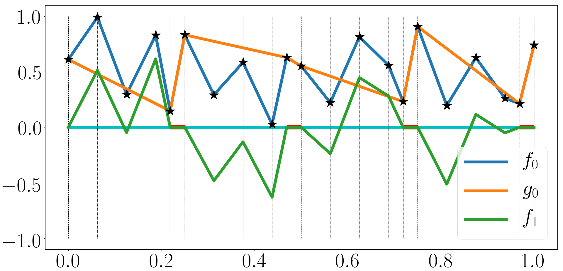
(a)

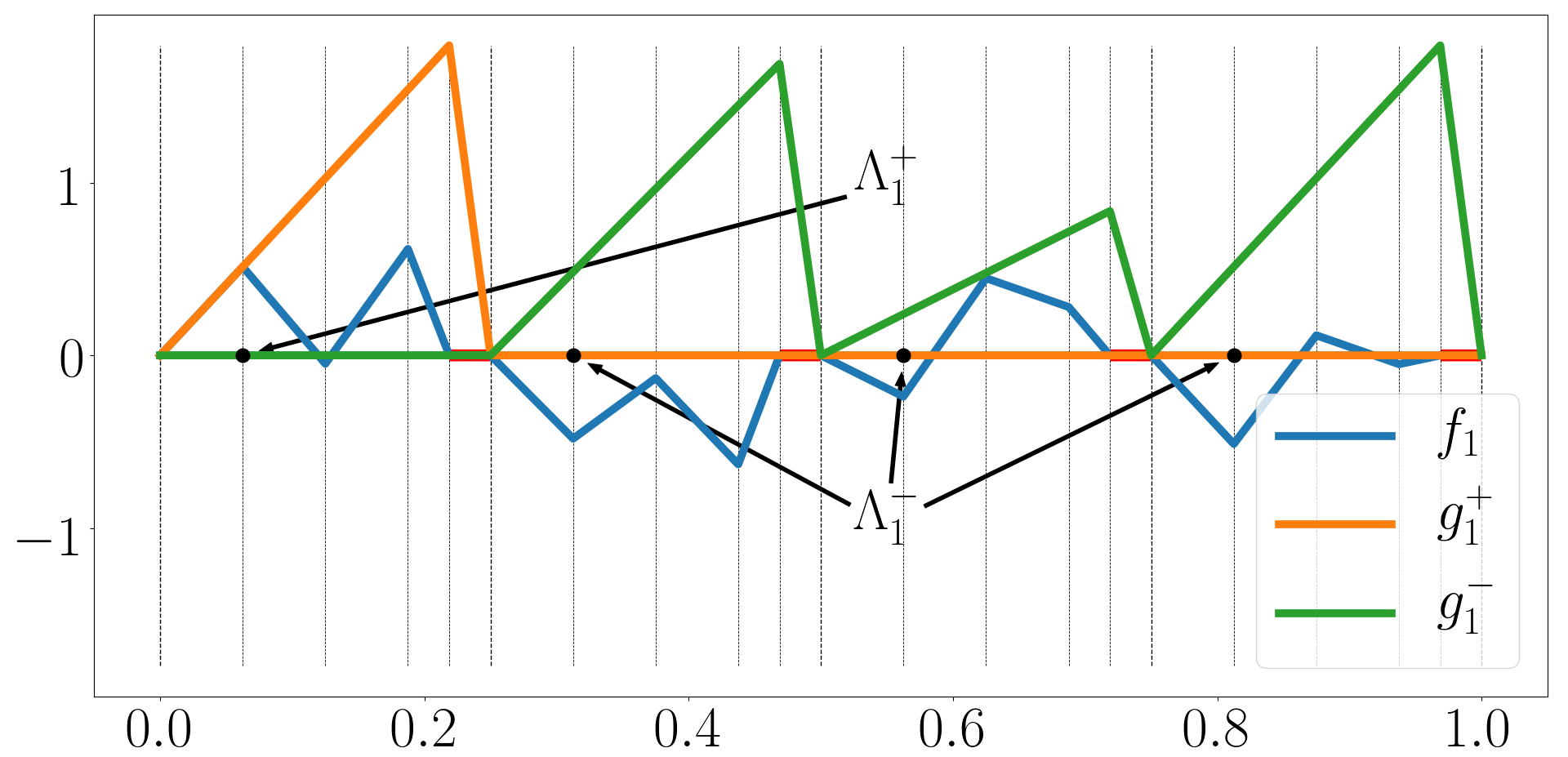
(b)

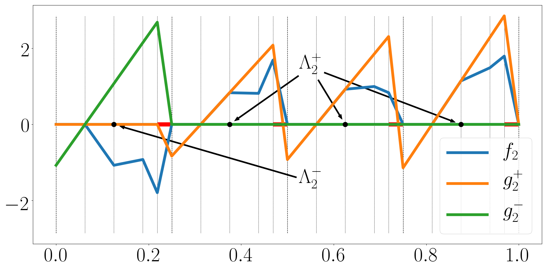
(c)

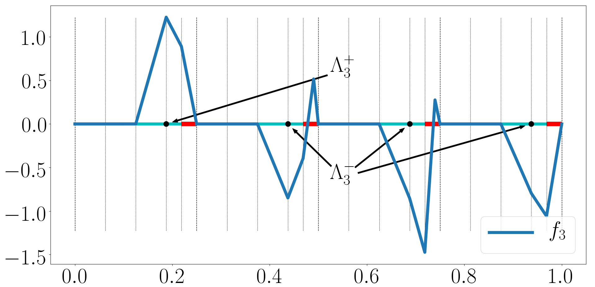
(d)

Figure 2: Illustrations of the proof of Lemma 2.2, especially Step $2$ of the proof, when $m=n=4$, with the “don’t-care” region in red. (a) Given samples $\{(x_{i},y_{i}):i=0,1,\cdots,m(n+1)\}$ marked with “star” signs, suppose $f_{0}(x)$ is a CPL function fitting the samples, construct $g_{0}$ such that $f_{1}=f_{0}-\sigma(g_{0})$ is closer to $0$ than $f_{0}$ in the $L^{\infty}$ sense. (b) Construct $g^{+}_{1}$ and $g^{-}_{1}$ such that $f_{2}=f_{1}-\sigma(g^{+}_{1})+\sigma(g^{-}_{1})$ is closer to $0$ than $f_{1}$ in the $L^{\infty}$ sense in a subset of the “important” region. (c) Construct $g^{+}_{2}$ and $g^{-}_{2}$ such that $f_{3}=f_{2}-\sigma(g^{+}_{2})+\sigma(g^{-}_{2})$ is closer to $0$ than $f_{2}$ in the $L^{\infty}$ sense in a larger subset of the “important” region. (d) The visualization of $f_{3}$, which is $0$ in the “important” areas that have been processed and may remain large near the “don’t-care” region. $f_{k}$ will decay quickly outside the “don’t-care” region as $k$ increases.

Step $2.2.2$: Determine $\bm{W}_{2}(2k,:)$ and $\bm{b}_{2}(2k)$.

By Lemma 2.1, we can choose $\bm{W}_{2}(2k,:)$ and $\bm{b}_{2}(2k)$ to fully determine $g^{+}_{k}(x)$ such that each $g^{+}_{k}(x_{i})$ matches a specific value for $i\in(I_{1}(m,n)-n-1)\cup(I_{1}(m,n)-1)\cup\{m(n+1)\}$. The values of $\big{\{}g^{+}_{k}(x_{i}):i\in(I_{1}(m,n)-n-1)\cup(I_{1}(m,n)-1)\cup\{m(n+1)\}\big{\}}$ are specified as:

• If $j\in\Lambda^{+}_{k}$, specify the values of $g^{+}_{k}(x_{j(n+1)})$ and $g^{+}_{k}(x_{j(n+1)+n})$ such that $g^{+}_{k}(x_{j(n+1)+k-1})=0$ and $g^{+}_{k}(x_{j(n+1)+k})=f_{k}(x_{j(n+1)+k})$. The existence of these values fulfilling the requirements above comes from the fact that $g^{+}_{k}(x)$ is linear on the interval $[x_{j(n+1)},x_{j(n+1)+n}]$ and $g^{+}_{k}(x)$ only depends on the values of $g^{+}_{k}(x_{j(n+1)+k-1})$ and $g^{+}_{k}(x_{j(n+1)+k})$ on $[x_{j(n+1)},x_{j(n+1)+n}]$. Now it is easy to verify that $\widetilde{g}^{+}_{k}(x):=\sigma(g^{+}_{k}(x))$ satisfies $\widetilde{g}^{+}_{k}(x_{j(n+1)+k})=f_{k}(x_{j(n+1)+k})\geq 0$ and $\widetilde{g}^{+}_{k}(x_{j(n+1)+\ell})=0$ for $\ell=0,1,\cdots,k-1$, and $\widetilde{g}^{+}_{k}$ is linear on each interval $[x_{j(n+1)+\ell},x_{j(n+1)+\ell+1}]$ for $\ell=0,1,\cdots,n-1$.

• If $j\in\Lambda^{-}_{k}$, let $g^{+}_{k}(x_{j(n+1)})=g^{+}_{k}(x_{j(n+1)+n})=0$. Then $\widetilde{g}^{+}_{k}(x)=0$ on the interval $[x_{j(n+1)},x_{j(n+1)+n}]$.

• Finally, specify the value of $g^{+}_{k}(x)$ at $x=x_{m(n+1)}$ as $0$.

Step $2.2.3$: Determine $\bm{W}_{2}(2k+1,:)$ and $\bm{b}_{2}(2k+1)$.

Similarly, we choose $\bm{W}_{2}(2k+1,:)$ and $\bm{b}_{2}(2k+1)$ such that $g^{-}_{k}(x)$ matches specific values as follows:

• If $j\in\Lambda^{-}_{k}$, specify the values of $g^{-}_{k}(x_{j(n+1)})$ and $g^{-}_{k}(x_{j(n+1)+n})$ such that $g^{-}_{k}(x_{j(n+1)+k-1})=0$ and $g^{-}_{k}(x_{j(n+1)+k})=-f_{k}(x_{j(n+1)+k})$. Then $\widetilde{g}^{-}_{k}(x):=\sigma(g^{-}_{k}(x))$ satisfies $\widetilde{g}^{-}_{k}(x_{j(n+1)+k})=-f_{k}(x_{j(n+1)+k})>0$ and $\widetilde{g}^{-}_{k}(x_{j(n+1)+\ell})=0$ for $\ell=0,1,\cdots,k-1$, and $\widetilde{g}^{-}_{k}(x)$ is linear on each interval $[x_{j(n+1)+\ell},x_{j(n+1)+\ell+1}]$ for $\ell=0,1,\cdots,n-1$.

• If $j\in\Lambda^{+}_{k}$, let $g^{-}_{k}(x_{j(n+1)})=g^{-}_{k}(x_{j(n+)+n})=0$. Then $\widetilde{g}^{-}_{k}(x)=0$ on the interval $[x_{j(n+1)},x_{j(n+1)+n}]$.

• Finally, specify the value of $g^{-}_{k}(x)$ at $x=x_{m(n+1)}$ as $0$.

Step $2.2.4$: Construct $f_{k+1}$ from $g^{+}_{k}$ and $g^{-}_{k}$.

For the sake of clarity, the properties of $g^{+}_{k}$ and $g^{-}_{k}$ constructed in Step $2.2.3$ are summarized below:

1. $f_{k}(x_{i})=\widetilde{g}_{k}^{+}(x_{i})=\widetilde{g}_{k}^{-}(x_{i})=0$ for $i\in\cup_{\ell=0}^{k-1}(I_{1}(m,n)-n-1+\ell)\cup\{m(n+1)\}$;

2. If $j\in\Lambda^{+}_{k}$,  $\widetilde{g}_{k}^{+}(x_{j(n+1)+k})=f_{k}(x_{j(n+1)+k})\geq 0$ and $\widetilde{g}_{k}^{-}(x_{j(n+1)+k})=0$;

3. If $j\in\Lambda^{-}_{k}$,  $\widetilde{g}_{k}^{-}(x_{j(n+1)+k})=-f_{k}(x_{j(n+1)+k})>0$ and $\widetilde{g}_{k}^{+}(x_{j(n+1)+k})=0$;

4. $\widetilde{g}_{k}^{+}$ and $\widetilde{g}_{k}^{-}$ are linear on each interval $[x_{j(n+1)+\ell},x_{j(n+1)+\ell+1}]$ for $\ell=0,1,\cdots,n-1,\ j\in\Lambda^{+}_{k}\cup\Lambda^{-}_{k}=\{0,1,\cdots,m-1\}$. In other words, $\widetilde{g}_{k}^{+}$ and $\widetilde{g}_{k}^{-}$ are linear on each interval $[x_{i-1},x_{i}]$ for $i\in I_{2}(m,n)\backslash\{0\}$.

See Figure 2 (a)-(c) for the illustration of $g_{0}$, $g^{+}_{1}$, $g^{-}_{1}$, $g^{+}_{2}$, and $g^{-}_{2}$, and to verify their properties as listed above.

Note that $\Lambda^{+}_{k}\cup\Lambda^{-}_{k}=\{0,1,\cdots,m-1\}$, so $f_{k}(x_{i})-\widetilde{g}_{k}^{+}(x_{i})+\widetilde{g}_{k}^{-}(x_{i})=0$ for $i\in\cup_{\ell=0}^{k}(I_{1}(m,n)-n-1+\ell)\cup\{m(n+1)\}$. Now we define $f_{k+1}:=f_{k}-\widetilde{g}^{+}_{k}+\widetilde{g}^{-}_{k}$, then

• $f_{k+1}(x_{i})=0$ for $i\in\cup_{\ell=0}^{k}(I_{1}(m,n)-n-1+\ell)\cup\{m(n+1)\}$;

• $f_{k+1}$ is linear on each interval $[x_{i-1},x_{i}]$ for $i\in I_{2}(m,n)\backslash\{0\}$.

See Figure 2 (b)-(d) for the illustration of $f_{1}$, $f_{2}$, and $f_{3}$, and to verify their properties as listed just above. This finishes the mathematical induction process. As we can imagine based on Figure 2, when $k$ increases, the support of $f_{k}$ shrinks to the “don’t-care” region.

Step $3$: Determine $\bm{W}_{3}$ and $\bm{b}_{3}$.

With the special vector function $\bm{g}=[g_{0},g_{1}^{+},g_{1}^{-},\cdots,g_{n}^{+},g_{n}^{-}]^{T}$ constructed in Step $2$, we are able to specify $\bm{W}_{3}$ and $\bm{b}_{3}$ to generate a desired $\phi(x)$ with a well-controlled $L^{\infty}$-norm matching the samples $\{(x_{i},y_{i})\}_{0\leq i\leq m(n+1)}$.

In fact, we can simply set $\bm{W}_{3}=[1,1,-1,1,-1,\cdots,1,-1]\in\mathbb{R}^{1\times(2n+1)}$ and $\bm{b}_{3}=0$, which finishes the construction of $\phi(x)$. The rest of the proof is to verify the properties of $\phi(x)$. Note that $\phi=\widetilde{g}_{0}+\sum_{\ell=1}^{n}\widetilde{g}^{+}_{\ell}-\sum_{\ell=1}^{n}\widetilde{g}^{-}_{\ell}$. By the mathematical induction, we have:

• $f_{n+1}=f_{0}-\widetilde{g}_{0}-\sum_{\ell=1}^{n}\widetilde{g}^{+}_{\ell}+\sum_{\ell=1}^{n}\widetilde{g}^{-}_{\ell}$;

• $f_{n+1}(x_{i})=0$ for $i\in\cup_{\ell=0}^{n}(I_{1}(m,n)-n-1+\ell)\cup\{m(n+1)\}=I_{0}(m,n)$;

• ${f}_{n+1}$ is linear on each interval $[x_{i-1},x_{i}]$ for $i\in I_{2}(m,n)\backslash\{0\}$.

Hence, $\phi=\widetilde{g}_{0}+\sum_{\ell=1}^{n}\widetilde{g}^{+}_{\ell}-\sum_{\ell=1}^{n}\widetilde{g}^{-}_{\ell}=f_{0}-f_{n+1}$. Then $\phi$ satisfies Conditions $(1)$ and $(2)$ of this lemma. It remains to check that $\phi$ satisfies Condition $(3)$.

By the definition of $f_{1}$, we have

$$\sup_{x\in[x_{0},\,x_{m(n+1)}]}|f_{1}(x)|\leq 2\max\{y_{i}:i\in I_{0}(m,n)\}.$$ (2.2)

By the induction process in Step $2$, for $k\in\{1,2,\cdots,n\}$, it holds that

$$\sup_{x\in[x_{0},\,x_{m(n+1)}]}|\widetilde{g}^{+}_{k}(x)|\leq\tfrac{\max\{x_{j(n+1)+n}-x_{j(n+1)+k-1}:j=0,1,\cdots,m-1\}}{\min\{x_{j(n+1)+k}-x_{j(n+1)+k-1}:j=0,1,\cdots,m-1\}}\sup_{x\in[x_{0},\,x_{m(n+1)}]}|f_{k}(x)|$$ (2.3)

and

$$\sup_{x\in[x_{0},\,x_{m(n+1)}]}|\widetilde{g}^{-}_{k}(x)|\leq\tfrac{\max\{x_{j(n+1)+n}-x_{j(n+1)+k-1}:j=0,1,\cdots,m-1\}}{\min\{x_{j(n+1)+k}-x_{j(n+1)+k-1}:j=0,1,\cdots,m-1\}}\sup_{x\in[x_{0},\,x_{m(n+1)}]}|f_{k}(x)|.$$ (2.4)

Since either $\widetilde{g}^{+}_{k}(x)$ or $\widetilde{g}^{-}_{k}(x)$ is equal to $0$ on $[0,1]$, we have

$$\sup_{x\in[x_{0},\,x_{m(n+1)}]}|\widetilde{g}^{+}_{k}(x)-\widetilde{g}^{-}_{k}(x)|\leq\tfrac{\max\{x_{j(n+1)+n}-x_{j(n+1)+k-1}:j=0,1,\cdots,m-1\}}{\min\{x_{j(n+1)+k}-x_{j(n+1)+k-1}:j=0,1,\cdots,m-1\}}\sup_{x\in[x_{0},\,x_{m(n+1)}]}|f_{k}(x)|.$$ (2.5)

Note that $f_{k+1}=f_{k}-\widetilde{g}^{+}_{k}+\widetilde{g}^{-}_{k}$, which means

$$\begin{split}\sup_{x\in[x_{0},\,x_{m(n+1)}]}|f_{k+1}(x)|&\leq\sup_{x\in[x_{0},\,x_{m(n+1)}]}|\widetilde{g}^{+}_{k}(x)-\widetilde{g}^{-}_{k}(x)|+\sup_{x\in[x_{0},\,x_{m(n+1)}]}|f_{k}(x)|\\ &\leq\left(\tfrac{\max\{x_{j(n+1)+n}-x_{j(n+1)+k-1}:j=0,1,\cdots,m-1\}}{\min\{x_{j(n+1)+k}-x_{j(n+1)+k-1}:j=0,1,\cdots,m-1\}}+1\right)\sup_{x\in[x_{0},\,x_{m(n+1)}]}|f_{k}(x)|\end{split}$$ (2.6)

for $k\in\{1,2,\cdots,n\}$. Then we have

$$\begin{split}\sup_{x\in[x_{0},\,x_{m(n+1)}]}|f_{n+1}(x)|\leq 2\max_{i\in I_{0}(m,n)}y_{i}\prod_{k=1}^{n}\left(\tfrac{\max\{x_{j(n+1)+n}-x_{j(n+1)+k-1}:j=0,1,\cdots,m-1\}}{\min\{x_{j(n+1)+k}-x_{j(n+1)+k-1}:j=0,1,\cdots,m-1\}}+1\right).\end{split}$$

Hence

$$\begin{split}\sup_{x\in[x_{0},\,x_{m(n+1)}]}|\phi(x)|&\leq\sup_{x\in[x_{0},\,x_{m(n+1)}]}|f_{0}(x)|+\sup_{x\in[x_{0},\,x_{m(n+1)}]}|f_{n+1}(x)|\\ &\leq 3\max_{i\in I_{0}(m,n)}y_{i}\prod_{k=1}^{n}\left(\tfrac{\max\{x_{j(n+1)+n}-x_{j(n+1)+k-1}:j=0,1,\cdots,m-1\}}{\min\{x_{j(n+1)+k}-x_{j(n+1)+k-1}:j=0,1,\cdots,m-1\}}+1\right).\end{split}$$

So, we finish the proof.

3 Main Results

We present our main results in this section. First, we quantitatively prove an achievable approximation rate in the $N$-term nonlinear approximation by construction, i.e., the lower bound of the approximation rate. Second, we show a lower bound of the approximation rate asymptotically, i.e., no approximant exists asymptotically following the approximation rate. Finally, we discuss the efficiency of the nonlinear approximation considering the approximation rate and parallel computing in FNNs together.

3.1 Quantitative Achievable Approximation Rate

Theorem 3.1.

For any $N\in\mathbb{N}^{+}$ and $f\in\textnormal{Lip}(\nu,\alpha,d)$ with $\alpha\in(0,1]$, we have:

1. If $d=1$, $\exists\ \phi\in\textnormal{NN}(\textnormal{\#input}=1;\,\textnormal{widthvec}=[2N,2N+1])$ such that

   $$\|\phi-f\|_{L^{1}([0,1])}\leq 2\nu N^{-2\alpha},\quad\textnormal{ for any }\ N\in\mathbb{N}^{+};$$

2. If $d>1$, $\exists\ \phi\in\textnormal{NN}(\textnormal{\#input}=d;\,\textnormal{widthvec}=[2d\lfloor N^{2/d}\rfloor,2N+2,2N+3])$ such that

   $$\|\phi-f\|_{L^{1}([0,1]^{d})}\leq 2(2\sqrt{d})^{\alpha}\nu N^{-2\alpha/d},\quad\textnormal{ for any }\ N\in\mathbb{N}^{+}.$$

Proof 3.2.

Without loss of generality, we assume $f(\bm{0})=0$ and $\nu=1$.

Step $1$: The case $d=1$.

Given any $f\in\textnormal{Lip}(\nu,\alpha,d)$ and $N\in\mathbb{N}^{+}$, we know $|f(x)|\leq 1$ for any $x\in[0,1]$ since $f(0)=0$ and $\nu=1$. Set $\bar{f}=f+1\geq 0$, then $0\leq\bar{f}(x)\leq 2$ for any $x\in[0,1]$. Let $X=\{\frac{i}{N^{2}}:i=0,1,\cdots,N^{2}\}\cup\{\frac{i}{N}-\delta:i=1,2,\cdots,N\}$, where $\delta$ is a sufficiently small positive number depending on $N$, and satisfying (3.2). Let us order $X$ as $x_{0}<x_{1}<\cdots<x_{N(N+1)}$. By Lemma 2.2, given the set of samples $\big{\{}(x_{i},\bar{f}(x_{i})):i\in\{0,1,\cdots,N(N+1)\}\big{\}}$, there exists $\phi\in\textnormal{NN}(\textnormal{\#input}=1;\,\textnormal{widthvec}=[2N,2N+1])$ such that

• $\phi(x_{i})=\bar{f}(x_{i})$ for $i=0,1,\cdots,N(N+1)$;

• $\phi$ is linear on each interval $[x_{i-1},x_{i}]$ for $i\notin\{(N+1)j:j=1,2,\cdots,N\}$;

• $\phi$ has an upper bound estimation: $\sup\{\phi(x):x\in[0,1]\}\leq 6(N+1)!$.

It follows that

$$|\bar{f}(x)-\phi(x)|\leq(x_{i}-x_{i-1})^{\alpha}\leq N^{-2\alpha},\quad\textnormal{if }x\in[x_{i-1},x_{i}],\quad\textnormal{for }i\notin\{(N+1)j:j=1,2,\cdots,N\}.$$

Define $H_{0}=\cup_{i\in\{(N+1)j:j=1,2,\cdots,N\}}[x_{i-1},x_{i}]$, then

$$|\bar{f}(x)-\phi(x)|\leq N^{-2\alpha},\quad\textnormal{ for any }x\in[0,1]\backslash H_{0},$$ (3.1)

by the fact that $\bar{f}\in\textnormal{Lip}(1,\alpha,d)$ and points in $X$ are equispaced. By $\mu(H_{0})\leq N\delta$, it follows that

$$\begin{split}\|\bar{f}-\phi\|_{L^{1}([0,1])}&=\int_{H_{0}}|\bar{f}(x)-\phi(x)|dx+\int_{[0,1]\backslash H_{0}}|\bar{f}(x)-\phi(x)|dx\\ &\leq N\delta(2+6(N+1)!)+N^{2}(N^{-2\alpha})N^{-2}\leq 2N^{-2\alpha},\end{split}$$

where the last inequality comes from the fact $\delta$ is small enough satisfying

$$N\delta(2+6(N+1)!)\leq N^{-2\alpha}.$$ (3.2)

Note that $f-(\phi-1)=f+1-\phi=\bar{f}-\phi$. Hence, $\phi-1\in\textnormal{NN}(\textnormal{\#input}=1;\,\textnormal{widthvec}=[2N,2N+1])$ and $\|f-(\phi-1)\|\leq 2N^{-2\alpha}$. So, we finish the proof for the case $d=1$.

Step $2$: The case $d>1$.

The main idea is to project the $d$-dimensional problem into a one-dimensional one and use the results proved above. For any $N\in\mathbb{N}^{+}$, let $n=\lfloor N^{2/d}\rfloor$ and $\delta$ be a sufficiently small positive number depending on $N$ and $d$, and satisfying (3.8). We will divide the $d$-dimensional cube into $n^{d}$ small non-overlapping sub-cubes (see Figure 3 for an illustration when $d=3$ and $n=3$), each of which is associated with a representative point, e.g., a vertex of the sub-cube. Due to the continuity, the target function $f$ can be represented by their values at the representative points. We project these representatives to one-dimensional samples via a ReLU FNN $\psi$ and construct a ReLU FNN $\bar{\phi}$ to fit them. Finally, the ReLU FNN $\phi$ on the $d$-dimensional space approximating $f$ can be constructed by $\phi=\bar{\phi}\circ\psi$. The precise construction can be found below.

By Lemma 2.1, there exists $\psi_{0}\in\textnormal{NN}(\textnormal{\#input}=1;\,\textnormal{widthvec}=[2n])$ such that

• $\psi_{0}(1)=n-1$, and $\psi_{0}(\tfrac{i}{n})=\psi_{0}(\tfrac{i+1}{n}-\delta)=i$ for $i=0,1,\cdots,n-1$;

• $\psi_{0}$ is linear between any two adjacent points of $\{\tfrac{i}{n}:i=0,1,\cdots,n\}\cup\{\tfrac{i}{n}-\delta:i=1,2,\cdots,n\}$.

Define the projection map $\psi$ by

$$\psi(\bm{x})=\sum_{i=1}^{d}\tfrac{1}{n^{i}}\psi_{0}(x_{i}),\quad\textnormal{for}\ \bm{x}=[x_{1},x_{2},\cdots,x_{d}]^{T}\in[0,1]^{d}.$$ (3.3)

Note that $\psi\in\textnormal{NN}(\textnormal{\#input}=1;\,\textnormal{widthvec}=[2dn])$. Given $f\in\textnormal{Lip}(\nu,\alpha,d)$, then $|f(\bm{x})|\leq\sqrt{d}$ for ${\bm{x}}\in[0,1]^{d}$ since $f(\bm{0})=0$, $\nu=1$, and $\alpha\in(0,1]$. Define $\bar{f}=f+\sqrt{d}$, then $0\leq\bar{f}(\bm{x})\leq 2\sqrt{d}$ for ${\bm{x}}\in[0,1]^{d}$. Hence, we have

$$\bigg{\{}\Big{(}\sum_{i=1}^{d}\tfrac{\theta_{i}}{n^{i}},\,\bar{f}(\tfrac{\bm{\theta}}{n})\Big{)}:{\bm{\theta}}=[\theta_{1},\theta_{2},\cdots,\theta_{d}]^{T}\in\{0,1,\cdots,n-1\}^{d}\bigg{\}}\cup\{(1,0)\}$$

as a set of $n^{d}+1$ samples of a one-dimensional function. By Lemma 2.1, $\exists\ \bar{\phi}\in\textnormal{NN}(\textnormal{\#input}=1;\,\textnormal{widthvec}=[2\lceil n^{d/2}\rceil,2\lceil n^{d/2}\rceil+1])$ such that

$$\bar{\phi}\Big{(}\sum_{i=1}^{d}\tfrac{\theta_{i}}{n^{i}}\Big{)}=\bar{f}\left(\tfrac{\bm{\theta}}{n}\right),\quad\textnormal{for}\ {\bm{\theta}}=[\theta_{1},\theta_{2},\cdots,\theta_{d}]^{T}\in\{0,1,\cdots,n-1\}^{d},$$ (3.4)

and

$$\sup_{t\in[0,1]}|\bar{\phi}(t)|\leq 6\sqrt{d}\left(\lceil n^{d/2}\rceil+1\right)!.$$ (3.5)

Since the range of $\psi$ on $[0,1]^{d}$ is a subset of $[0,1]$, $\exists\ \phi\in\textnormal{NN}\left(\textnormal{\#input}=d;\,\textnormal{widthvec}=[2nd,2\lceil n^{d/2}\rceil,2\lceil n^{d/2}\rceil+1]\right)$ defined via $\phi(\bm{x})=\bar{\phi}\scalebox{0.85}[0.85]{$\circ$}\psi(\bm{x})$ for ${\bm{x}}\in[0,1]^{d}$ such that

$$\sup_{{\bm{x}}\in[0,1]^{d}}|\phi(\bm{x})|\leq 6\sqrt{d}\left(\lceil n^{d/2}\rceil+1\right)!.$$ (3.6)

Define $H_{1}=\cup_{j=1}^{d}\left\{{\bm{x}}=[x_{1},x_{2},\cdots,x_{d}]^{T}\in[0,1]^{d}:x_{j}\in\cup_{i=1}^{n}[\tfrac{i}{n}-\delta,\tfrac{i}{n}]\right\}$, which separates the $d$-dimensional cube into $n^{d}$ important sub-cubes as illustrated in Figure 3. To index these $d$-dimensional smaller sub-cubes, define $Q_{\bm{\theta}}=\big{\{}{\bm{x}}=[x_{1},x_{2},\cdots,x_{d}]^{T}\in[0,1]^{d}:x_{i}\in[\tfrac{\theta_{i}}{n},\tfrac{\theta_{i}+1}{n}-\delta],\ i=1,2,\cdots,d\big{\}}$ for each $d$-dimensional index ${\bm{\theta}}=[\theta_{1},\theta_{2},\cdots,\theta_{d}]^{T}\in\{0,1,\cdots,n-1\}^{d}$. By (3.3), (3.4), and the definition of $\psi_{0}$, for any $\bm{x}=[x_{1},x_{2},\cdots,x_{d}]^{T}\in Q_{\bm{\theta}}$, we have $\phi(\bm{x})=\bar{\phi}(\psi(\bm{x}))=\bar{\phi}\Big{(}\sum_{i=1}^{d}\tfrac{1}{n^{i}}\psi_{0}(x_{i})\Big{)}=\bar{\phi}\Big{(}\sum_{i=1}^{d}\tfrac{1}{n^{i}}\theta_{i}\Big{)}=\bar{f}\left(\tfrac{\bm{\theta}}{n}\right)$. Then

$$|\bar{f}(\bm{x})-\phi(\bm{x})|=|\bar{f}(\bm{x})-\bar{f}\left(\tfrac{\bm{\theta}}{n}\right)|\leq(\sqrt{d}/n)^{\alpha},\quad\textnormal{for any}\ {\bm{x}}\in Q_{\bm{\theta}}.$$ (3.7)

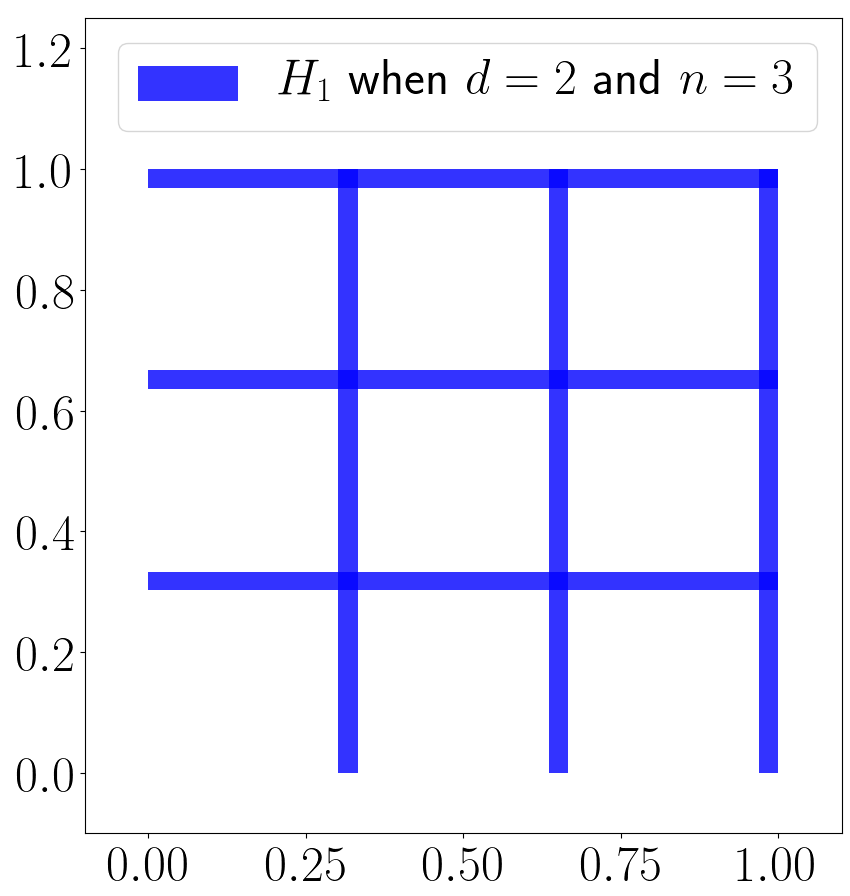
(a)

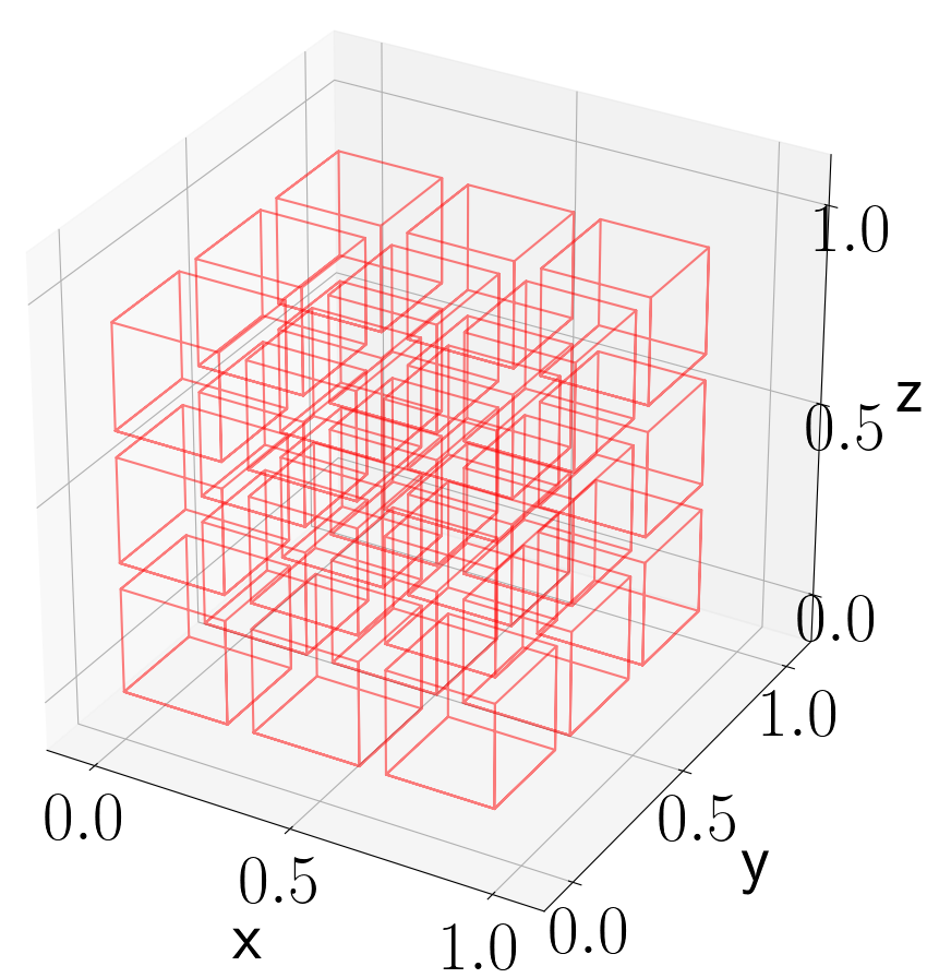
(b)

Figure 3: An illustration of $H_{1}$ and $n^{d}$ small non-overlapping sub-cubes that $H_{1}$ separates when $n=3$. (a) When $d=2$, $H_{1}$ in blue separates $[0,1]^{2}$ into $n^{d}=9$ sub-cubes. (b) When $d=3$, $H_{1}$ (no color) separates $[0,1]^{3}$ into $n^{d}=27$ sub-cubes in red.

Because $\mu(H_{1})\leq dn\delta$, $[0,1]^{d}=\cup_{\bm{\theta}\in\{0,1,\cdots,n-1\}^{d}}Q_{\bm{\theta}}\cup H_{1}$, (3.6), and (3.7), we have

$$\begin{split}\|\bar{f}-\phi\|_{L^{1}([0,1]^{d})}&=\int_{H_{1}}|\bar{f}-\phi|d{\bm{x}}+\int_{[0,1]^{d}\backslash H_{1}}|\bar{f}-\phi|d{\bm{x}}\\ &\leq\mu(H_{1})\Big{(}2\sqrt{d}+6\sqrt{d}\big{(}\lceil n^{d/2}\rceil+1\big{)}!\Big{)}+\sum_{\bm{\theta}\in\{0,1,\cdots,n-1\}^{d}}\int_{Q_{\bm{\theta}}}|\bar{f}-\phi|d{\bm{x}}\\ &\leq 2n\delta d\sqrt{d}\Big{(}1+3\big{(}\lceil n^{d/2}\rceil+1\big{)}!\Big{)}+\sum_{\bm{\theta}\in\{0,1,\cdots,n-1\}^{d}}(\sqrt{d}/n)^{\alpha}\mu(Q_{\bm{\theta}})\\ &\leq 2d^{\alpha/2}n^{-\alpha},\end{split}$$

where the last inequality comes from the fact that $\delta$ is small enough such that

$$2n\delta d\sqrt{d}\Big{(}1+3\big{(}\lceil n^{d/2}\rceil+1\big{)}!\Big{)}\leq d^{\alpha/2}n^{-\alpha}.$$ (3.8)

Note that $f-(\phi-\sqrt{d})=\bar{f}-\phi$. Hence, $\phi-\sqrt{d}\in\textnormal{NN}(\textnormal{\#input}=d;\,\textnormal{widthvec}=[2nd,2\lceil n^{d/2}\rceil,2\lceil n^{d/2}\rceil+1])$ and $\|f-(\phi-\sqrt{d})\|_{L^{1}([0,1]^{d})}\leq 2d^{\alpha/2}n^{-\alpha}$. Since $n=\lfloor N^{2/d}\rfloor$, we have $\lceil n^{d/2}\rceil\leq N+1$. Therefore,

$$\begin{split}\phi-\sqrt{d}&\in\textnormal{NN}(\textnormal{\#input}=d;\,\textnormal{widthvec}=[2d\lfloor N^{2/d}\rfloor,2N+2,2N+3])\\ \end{split}$$

and

$$\|f-(\phi-\sqrt{d})\|_{L^{1}([0,1]^{d})}\leq 2d^{\alpha/2}n^{-\alpha}=2d^{\alpha/2}\lfloor N^{2/d}\rfloor^{-\alpha}\leq 2d^{\alpha/2}(N^{2/d}/2)^{-\alpha}=2(2\sqrt{d})^{\alpha}N^{-2\alpha/d},$$

where the second inequality comes from the fact $\lfloor x\rfloor\geq\tfrac{x}{2}$ for $x\in[1,\infty)$. So, we finish the proof when $d>1$.

Theorem 3.1 shows that for $f\in\textnormal{Lip}(\nu,\alpha,d)$ ReLU FNNs with two or three function compositions can achieve the approximation rate $\mathcal{O}(\nu N^{-2\alpha/d})$. Following the same proof as in Theorem 3.1, we can show that:

Corollary 3.3.

$\forall\ m,n\in\mathbb{N}^{+}$, the closure of $\textnormal{NN}(\textnormal{\#input}=1;\,\textnormal{widthvec}=[2m,2n+1])$ contains $\textnormal{CPL}(mn+1)$ in the sense of $L^{1}$-norm.

An immediate implication of Corollary 3.3 is that, for any function $f$ on $[0,1]$, if $f$ can be approximated via one-hidden-layer ReLU FNNs with an approximation rate $\mathcal{O}(N^{-\eta})$ for any $\eta>0$, the rate can be improved to $\mathcal{O}(N^{-2\eta})$ via one more composition.

3.2 Asymptotic Unachievable Approximation Rate

In Section 3.1, we have analyzed the approximation capacity of ReLU FNNs in the nonlinear approximation for general continuous functions by construction. In this section, we will show that the construction in Section 3.1 is essentially and asymptotically tight via showing the approximation lower bound in Theorem 3.4 below.

Theorem 3.4.

For any $\ L\in\mathbb{N}^{+}$, $\rho>0$, and $C>0$, $\exists\ f\in\textnormal{Lip}(\nu,\alpha,d)$ with $\alpha\in(0,1]$, for all $N_{0}>0$, there exists $N\geq N_{0}$ such that

$$\inf_{\phi\in\textnormal{NN}(\textnormal{\#input}=d;\,\textnormal{maxwidth}\leq N;\,\textnormal{\#layer}\leq L)}\|\phi-f\|_{L^{\infty}([0,1]^{d})}\geq C\nu N^{-(2\alpha/d+\rho)}.$$