Online Learning with Continuous Ranked Probability Score

Abstract

We consider the case where several competing methods produce online predictions in the form of probability distribution functions. The dissimilarity between a probability forecast and an outcome is measured by a loss function (scoring rule). Popular example of scoring rule for continuous outcomes is Continuous Ranked Probability Score (${\rm CRPS}$). In this paper the problem of combining probabilistic forecasts is considered in the prediction with expert advice framework. We show that ${\rm CRPS}$ is a mixable loss function and then the time-independent upper bound for the regret of the Vovk’s aggregating algorithm using ${\rm CRPS}$ as a loss function can be obtained. Also, we incorporate in this scheme a smooth version of the method of specialized experts which allows us to make more flexible and accurate predictions. We present the results of numerical experiments illustrating the proposed methods.

1 Introduction

Probabilistic forecasts in the form of probability distributions over future events have become popular in several fields including meteorology, hydrology, economics, demography (see discussion in Jordan et al. 2018). Probabilistic predictions are used in the theory of conformal predictions, where a predictive distribution that is valid under a nonparametric assumption can be assigned to any forecasting algorithm (see Vovk et al. 2019).

The dissimilarity between a probability forecast and an outcome is measured by a loss function (scoring rule). Popular example of scoring rule for continuous outcomes is Continuous Ranked Probability Score (${\rm CRPS}$).

$${\rm CRPS}(F,y)=\int(F(u)-H(u-y))^{2}du,$$

where $F(u)$ is a probability distribution function, $y$ is an outcome – a real number, and $H(x)$ is the Heaviside function: $H(x)=0$ for $x<0$ and $H(x)=1$ for $x\geq 0$

We consider the case where several competing methods produce online predictions in the form of probability distribution functions. These predictions can lead to large or small losses. Our task is to combine these forecasts into one optimal forecast, which will lead to the smallest possible loss in the framework of the available past information.

We solve this problem in the prediction with expert advice (PEA) framework. We consider the game-theoretic on-line learning model in which a learner (aggregating) algorithm has to combine predictions from a set of $N$ experts (see e.g. Littlestone and Warmuth 1994, Freund and Schapire 1997, Vovk 1990, Vovk 1998,  Cesa-Bianchi and Lugosi 2006 among others).

In contrast to the standard PEA approach, we consider the case where each expert presents probability distribution functions rather than a point prediction. The learner presents his forecast also in a form of probability distribution function computed using probabilistic predictions presented by the experts.

In online setting, at each time step $t$ any expert issues a probability distribution as a forecast. The aggregating algorithm combines these forecasts into one aggregated forecast, which is a probability distribution function. The effectiveness of the aggregating algorithm on any time interval $[1,T]$ is measured by the regret which is the difference between the cumulated loss of the aggregating algorithm and the cumulated loss of the best expert suffered on first $T$ steps.

There are a lot of papers on probabilistic predictions and on ${\rm CRPS}$ scoring rule (some of them are Brier 1950, Bröcker et al. 2007, Bröcker et al. 2008, Bröcker 2012, Epstein 1969, Jordan et al. 2018, Raftery et al. 2005). Most of them referred to the ensemble interpretation models. In some cases, experts use for their predictions probability distributions functions (data models) which are defined explicitly in an analytic form. In this paper we propose the rules for aggregation of such the probability distributions functions. We present the exact formulas for direct calculation of the aggregated probability distribution function given probability distribution functions presented by the experts.

In this paper we obtain a tight upper bound of the regret for a special case when the outcomes and the probability distributions are located in a finite interval $[a,b]$ of real line. We show that the loss function ${\rm CRPS}(F,y)$ is mixable in sense of Vovk (1998) and apply the Vovk’s aggregating algorithm to obtain the time-independent upper bound $\frac{b-a}{2}\ln N$ for the regret.

The application we will consider below in Section 5 (which is the sequential short-term (one-hour-ahead) forecasting of probability distribution function of electricity consumption) will take place in a variant of the basic problem of prediction with expert advice called prediction with specialized (or sleeping) experts. At each round only some of the experts output a prediction while the other ones are inactive. Each expert is expected to provide accurate forecasts mostly in given external conditions, that can be known beforehand. For instance, in the case of the prediction of electricity consumption, experts can be specialized to a season, temperature, to time of day.

In Section 4 we prove that the ${\rm CRPS}$ function is mixable and then all machinery of the Vovk (1998) aggregating algorithm (AA) and of the exponentially weighted average forecaster (WA) can be applied (see Cesa-Bianchi and Lugosi 2006).

In Section 4 we present a method for computing online the aggregated probability distribution function given the probability distribution functions presented by the experts and prove a time-independent bound for the regret of the proposed algorithm.

The method of specialized experts was first proposed by Freund et al. (1997) and further developed by Chernov and Vovk (2009), Devaine et al. (2013), Kalnishkan et al. (2015). With this approach, at each step $t$, a set of specialized experts $E_{t}\subseteq\{1,\dots,N\}$ be given. A specialized expert $i$ issues its forecasts not at all steps $t=1,2,\dots$, but only when $i\in E_{t}$. At any step, the aggregating algorithm uses forecasts of only “active (non-sleeping)” experts.

The second contribution of this paper is that we have incorporated into the aggregating algorithm a smooth generalization of the method of specialized experts (Sections 3 and 5.2). At each time moment $t$, we complement the expert $i$ forecast by a confidence level which is a real number $p_{i,t}\in[0,1]$. In particular, $p_{i,t}=1$ means that the forecast of the expert $i$ is used in full, whereas in the case of $p_{i,t}=0$ it is not taken into account at all (the expert sleeps). In cases where $0<p_{i,t}<1$ the expert’s forecast is partially taken into account. For example, when moving from one season to another, an expert tuned to the previous season gradually loses his predictive abilities. The dependence of $p_{i,t}$ on values of exogenous parameters can be predetermined by a specialist in the domain or can be constructed using regression analysis on historical data.

We demonstrate the effectiveness of the proposed methods in Section 5, where the results of numerical experiments with synthetic and real data are presented.

2 Preliminaries

In this section we present the main definitions and the auxiliary results of the theory of prediction with expert advice, namely, learning with mixable loss functions.

2.1 Online learning

Let a set of outcomes $\Omega$ and a set $\Gamma$ of forecasts (decision space) be given. We consider the learning with a loss function $\lambda(f,y)$, where $f\in\Gamma$ and $y\in\Omega$. Let also, a set $E$ of experts be given. For simplicity we assume that $E=\{1,\dots,N\}$.

In PEA approach the learning process is represented as a game. The experts and the learner observe past real outcomes generated online by some adversarial mechanism (called nature) and present their forecasts. After that, a current outcome is revealed by the nature.

At any round $t=1,2,\dots$ each expert $i\in E$ presents a forecast $f_{i,t}\in\Gamma$, then the learner presents its forecast $f_{t}\in\Gamma$, after that, an outcome $y_{t}\in\Omega$ will be revealed. Each expert $i$ suffers the loss $\lambda(f_{i,t},y_{t})$ and the learner suffers the loss $\lambda(f_{t},y_{t})$; see Protocol 1 below.

Protocol 1

  

FOR $t=1,\dots,T$

1. Receive the experts’ predictions $f_{i,t}$, where $1\leq i\leq N$.

2. Present the learner’s forecast $f_{t}$.

3. Observe the true outcome $y_{t}$ and compute the losses $\lambda(f_{i,t},y_{t})$ of the experts and the loss $\lambda(f_{t},y_{t})$ of the learner.

ENDFOR   

Let $H_{T}=\sum\limits_{t=1}^{T}\lambda(f_{t},y_{t})$ be the cumulated loss of the learner and $L^{i}_{T}=\sum\limits_{t=1}^{T}\lambda(f_{i,t},y_{t})$ be the cumulated loss of an expert $i$. The difference $R^{i}_{T}=H_{T}-L^{i}_{T}$ is called regret with respect to an expert $i$ and $R_{T}=H_{T}-\min_{i}L^{i}_{T}$ is the regret with respect to the best expert. The goal of the learner is to minimize the regret.

2.2 Aggregating Algorithm (AA)

The Vovk’s Aggregating algorithm (Vovk 1990, Vovk 1998) is the base algorithm for computing the learner predictions. This algorithm starting from the initial weights $w_{i,1}$ (usually $w_{i,1}=\frac{1}{N}$ for all $i$) assign weights $w_{i,t}$ for the experts $i\in E$ using the weights update rule:

$$w_{i,t+1}=w_{i,t}e^{-\eta\lambda(f_{i,t},y_{t})}\mbox{ for }t=1,2,\dots,$$ (1)

where $\eta>0$ is a learning rate. The normalized weights are defined

$$w^{*}_{i,t}=\frac{w_{i,t}}{\sum\limits_{j=1}^{N}w_{j,t}}.$$ (2)

The main tool of AA is a superprediction function

$$g_{t}(y)=-\frac{1}{\eta}\ln\sum\limits_{i=1}^{N}e^{-\eta\lambda(f_{i,t},y)}w^{*}_{i,t}.$$ (3)

We consider probability distributions ${\bf q}=(q_{1},\dots,q_{N})$ on the set $E$ of the experts: $\sum\limits_{i=1}^{N}q_{i}=1$ and $q_{i}\geq 0$ for all $i$. By Vovk (1998) a loss function is called $\eta$-mixable if for any probability distribution ${\bf q}$ on the set $E$ of experts and for any predictions ${\bf c}=(c_{1},\dots,c_{N})$ of the experts there exists a forecast $f$ such that

$$\lambda(f,y)\leq g(y)\mbox{ for all }y,$$ (4)

where

$$g(y)=-\frac{1}{\eta}\ln\sum\limits_{i=1}^{N}e^{-\eta\lambda(c_{i},y)}q_{i}.$$ (5)

We fix some rule for calculating a forecast $f$ and write

$$f={\rm Subst}({\bf c},{\bf q}).$$ (6)

The function ${\rm Subst}$ is called the substitution function.

As follows from (4) and (5) if a loss function $\lambda(f,y)$ is $\eta$-mixable then the loss function $c\lambda(f,y)$ is $\frac{\eta}{c}$-mixable for any $c>0$.

Regret analysis for AA. Assume that a loss function $\lambda(f,y)$ is $\eta$-mixable. Let ${\bf w}^{*}_{t}=(w^{*}_{1,t},\dots,w^{*}_{N,t})$ be the normalized weights and ${\bf f}_{t}=(f_{1,t},\dots,f_{N,t})$ be the experts’ forecasts at step $t$. Define in Protocol 1 the learner’s forecast $f_{t}={\rm Subst}({\bf f}_{t},{\bf w}^{*}_{t})$. By (4) $\lambda(f_{t},y_{t})\leq g_{t}(y_{t})$ for all $t$, where $g_{t}(y)$ is defined by (3).

Let $H_{T}=\sum\limits_{t=1}^{T}\lambda(f_{t},y_{t})$ be the cumulated loss of the learner and $L^{i}_{T}=\sum\limits_{t=1}^{T}\lambda(f_{i,t},y_{t})$ be the cumulated loss of an expert $i$. By definition $g_{t}(y_{t})=-\frac{1}{\eta}\ln\frac{W_{t+1}}{W_{t}}$, where $W_{t}=\sum\limits_{i=1}^{N}w_{i,t}$ and $W_{1}=1$. By the weight update rule (1) we obtain $w_{i,t+1}=\frac{1}{N}e^{-\eta L^{i}_{t}}$.

By telescoping, we obtain the time-independent bound

$$H_{T}\leq\sum\limits_{t=1}^{T}g_{t}(y_{t})=-\frac{1}{\eta}\ln W_{T+1}\leq L^{i}_{T}+\frac{\ln N}{\eta}$$ (7)

for any expert $i$. Therefore, there is a strategy for the learner that guarantees $R_{T}\leq\frac{\ln N}{\eta}$ for all $T$.

Exponential concave loss functions. Assume that the set of all forecasts form a linear space. In this case, the mixability is a generalization of the notion of the exponential concavity. A loss function $\lambda(f,y)$ is called $\eta$-exponential concave if for each $\omega$ the function $\exp(-\eta\lambda(f,y))$ is concave by $f$ for any $y$ (see Cesa-Bianchi and Lugosi 2006). For exponential concave loss function the inequality $\lambda(f,y)\leq g(y)$ holds for all $y$ by definition, if the forecast of the learner is computed using the weighted average (WA) of the experts predictions:

$$f=\sum\limits_{i=1}^{N}q_{i}f_{i},$$ (8)

where ${\bf q}=(q_{1},\dots,q_{N})$ is a probability distribution on the set of experts, and $f_{1},\dots,f_{N}$ are theirs forecasts.

For exponential concave loss function and the game defined by Protocol 1, where the learner’s forecast is computed by (8), we also have the time-independent bound (7) for the regret.

Square loss function. The important special case is $\Omega=\{0,1\}$ and $\Gamma=[0,1]$. The square loss function $\lambda(\gamma,\omega)=(\gamma-\omega)^{2}$ is $\eta$-mixable loss function for any $0<\eta\leq 2$, where $\gamma\in[0,1]$ and $\omega\in\{0,1\}$. In this case, at any step $t$, the corresponding forecast $f_{t}$ (in Protocol 1) can be defined as

$$f_{t}={\rm Subst}({\bf f}_{t},{\bf w}^{*}_{t})=\frac{1}{2}-\frac{1}{2\eta}\ln\frac{\sum\limits_{i=1}^{N}w^{*}_{i,t}e^{-\eta\lambda(f_{i,t},0)}}{\sum\limits_{i=1}^{N}w^{*}_{i,t}e^{-\eta\lambda(f_{i,t},1)}},$$ (9)

where ${\bf f}_{t}=(f_{1,t},\dots,f_{N,t})$ is the vector of the experts’ forecasts and ${\bf w}^{*}_{t}=(w^{*}_{1,t},\dots,w^{*}_{N,t})$ is the vector of theirs normalized weights defined by (1) and (2). We refer the reader for details to Vovk (1990), Vovk (1998), and Vovk (2001).

The square loss function $\lambda(f,\omega)=(f-\omega)^{2}$, where $\omega\in\{0,1\}$ and $f\in[0,1]$, is $\eta$-exponential concave for any $0<\eta\leq\frac{1}{2}$ (see Cesa-Bianchi and Lugosi 2006).

3 AA for experts with confidence

In this section we consider an extended setting. At each time moment $t$ the forecasts ${\bf f}_{t}=(f_{1,t},\dots f_{N,t})$ of the experts and confidence levels ${\bf p}_{t}=(p_{1,t},\dots,p_{N,t})$ of these forecasts are revealed.

Each confidence level is a number between 0 and 1. If $p_{i,t}=0$ then the corresponding expert “sleeps” at step $t$ and its forecast is not taken into account. If $p_{i,t}<1$ then we will use the forecast $f_{i,t}$ only partially. Confidence levels can be set by the expert itself or by the learner.

To take into account confidence levels, we use the fixed point method by Chernov and Vovk (2009). We consider any confidence level $p_{i,t}$ as a probability distribution ${\bf p}_{i,t}=(p_{i,t},1-p_{i,t})$ on a two element set. Define the auxiliary forecast:

$$\tilde{f}_{i,t}=\left\{\begin{array}[]{l}f_{i,t}\mbox{ with probability }p_{i,t},\\ f_{t}\mbox{ with probability }1-p_{i,t},\end{array}\right.$$

where $f_{t}$ is a forecast of the learner.

First, we provide a justification of the algorithm presented below. Our goal is to define the forecast $f_{t}$ such that

$$e^{-\eta\lambda(f_{t},y)}\geq\sum_{i=1}^{N}E_{{\bf p}_{i,t}}[e^{-\eta\lambda(\tilde{f}_{i,t},y)}]w_{i,t}$$ (10)

for each $y$. Here $E_{{\bf p}_{i,t}}$ is the mathematical expectation with respect to the probability distribution ${\bf p}_{i,t}$. Also, $w_{i,t}$ is the weight of the expert $i$ accumulated at the end of step $t$.

We rewrite inequality (10) in a more detailed form:

$$e^{-\eta\lambda(f_{t},y)}\geq\sum_{i=1}^{N}E_{{\bf p}_{i,t}}[e^{-\eta\lambda(\tilde{f}_{i,t},y)}]w_{i,t}=$$ (11)

$$\sum_{i=1}^{N}p_{i,t}w_{i,t}e^{-\eta\lambda(f_{i,t},y)}+e^{-\eta\lambda(f_{t},y)}\left(1-\sum_{i=1}^{N}p_{i,t}w_{i,t}\right)$$ (12)

for all $\omega$. Therefore, the inequality (10) is equivalent to the inequality

$$e^{-\eta\lambda(f_{i},y)}\geq\sum_{i=1}^{N}w^{*}_{i,t}e^{-\eta\lambda(f_{i,t},y)},$$ (13)

where

$$w^{*}_{i,t}=\frac{p_{i,t}w_{i,t}}{\sum_{j=1}^{N}p_{j,t}w_{j,t}}.$$ (14)

According to the rule (6) for computing the forecast of AA define $f_{t}={\rm Subst}({\bf f}_{t},{\bf w}^{*}_{t})$. Then (13) and its equivalent (11) are valid. Here ${\rm Subst}$ is the substitution function, ${\bf w}^{*}_{t}=(w^{*}_{i,1},\dots,w^{*}_{i,N})$ and ${\bf f}_{t}=(f_{1,t},\dots f_{i,N})$.

Now, we present the analogue of Protocol 1 for AA with confidence.

Protocol 1a

  

FOR $t=1,\dots,T$

1. Receive the experts’ predictions $f_{i,t}$ and confidence levels $p_{i,t}$, where $1\leq i\leq N$.

2. Present the learner’s forecast $f_{t}={\rm Subst}({\bf f}_{t},{\bf w}^{*}_{t}))$, where normalized weights ${\bf w}^{*}_{t}=(w^{*}_{1,t},\dots,w^{*}_{N,t})$ are defined by (14).

3. Observe the true outcome $y_{t}$ and compute the losses $l_{i,t}=\lambda(f_{i,t},y_{t})$ of the experts and the loss $\lambda(f_{t},y_{t})$ of the learner.

4. Update the weights (of the virtual experts) by the rule

   $$w_{i,t+1}=w_{i,t}e^{-\eta(p_{i,t}\lambda(f_{i,t},y_{t})+(1-p_{i,t})\lambda(f_{t},y_{t}))}$$ (15)

ENDFOR   

Let $h_{t}=\lambda(f_{t},y_{t})$ be the loss of the learner at time moment $t$, $\tilde{l}_{i,t}=\lambda(\tilde{f}_{i,t},y_{t})$ be the estimated loss of an expert $i$, and $\hat{l}_{i,t}=E_{{\bf p}_{i,t}}[\tilde{l}_{i,t}]$ be its expectation. By virtual expert we mean the expert which suffers the loss $\hat{l}_{i,t}$.

Since by definition $\hat{l}_{i,t}=p_{i,t}l_{i,t}+(1-p_{i,t})h_{t}$, we have $h_{t}-\hat{l}_{i,t}=p_{i,t}(h_{t}-l_{i,t})$. We call the last quantity discounted excess loss with respect to an expert $i$ at a time moment $t$ and we will measure the performance of our algorithm by the cumulative discounted excess loss with respect to any expert $i$.

Theorem 1

For any ${1\leq i\leq N}$, the following upper bound for the cumulative excess loss (discounted regret) holds true:

$$\sum\limits_{t=1}^{T}p_{i,t}(h_{t}-l_{i,t})\leq\frac{\ln N}{\eta}.$$ (16)

Proof. By convexity of the exponent the inequality (10) implies

$$e^{-\eta\lambda(f_{t},y)}\geq\sum_{i=1}^{N}e^{-\eta E_{{\bf p}_{i,t}}[\lambda(\tilde{f}_{i,t},y)]}w^{*}_{i,t}=\sum_{i=1}^{N}e^{-\eta\hat{l}_{i,t}}w^{*}_{i,t}.$$ (17)

Let $m_{t}=-\frac{1}{\eta}\ln\sum_{i=1}^{N}w^{*}_{i,t}e^{-\eta\hat{l}_{i,t}}$. By (17) $h_{t}\leq m_{t}$. Rewrite the update rule (15) as

$$w_{i,t+1}=w_{i,t}e^{-\eta\hat{l}_{i,t}}.$$ (18)

Recall that $W_{T}=\sum_{t=1}w_{i,t}$, $W_{1}=1$ and $m_{t}=\frac{1}{\eta}\ln\frac{W_{t+1}}{W_{t}}$. As in (7), using (17) and (18), we obtain

$$\sum_{t=1}^{T}h_{t}\leq\sum_{t=1}^{T}m_{t}=-\frac{1}{\eta}\ln W_{T+1}\leq\sum_{t=1}^{T}\hat{l}_{i,t}+\frac{\ln N}{\eta}$$

for any $i$. Since $h_{t}-\hat{l}_{i,t}=p_{i,t}(h_{t}-l_{i,t})$, the inequality (16) follows. QED

4 Aggregation of probability forecasts

4.1 ${\rm CRPS}$ loss function

Let in Protocol 1 the set of outcomes be an interval $\Omega=[a,b]$ of the real line for some $a<b$ and the set of forecasts $\Gamma$ be a set of all probability distribution functions $F:[a,b]\to[0,1]$.

The quality of the prediction $F$ in view of the actual outcome $y$ is often measured by the continuous ranked probability score (loss function)

$${\rm CRPS}(F,y)=\int_{a}^{b}(F(u)-H(u-y))^{2}du,$$ (19)

where $H(x)$ is the Heaviside function: $H(x)=0$ for $x<0$ and $H(x)=1$ for $x\geq 0$ (Epstein (1969), Matheson and Winkler 1976, etc).

For simplicity in this definition, we consider integration over a finite interval. Such definition is closer to practical applications and allows a more elementary theoretical analysis. More general definition includes a density $\mu(u)$ and integration over the real line:

$${\rm CRPS}(F,y)=\int_{-\infty}^{+\infty}(F(u)-H(u-y))^{2}\mu(u)du.$$ (20)

The definition (19) is a special case of this definition (up to a factor), where $\mu(u)=\frac{1}{b-a}$ for $u\in[a,b]$ and $\mu(u)=0$ otherwise. In can be proved that the function (20) is $\eta$-mixable for $0<\eta\leq 2$ and $\eta$-exponentially concave for $0<\eta\leq\frac{1}{2}$ (see Korotin et al. 2019).

The ${\rm CRPS}$ score measures the difference between the forecast $F$ and a perfect forecast $H(u-y)$ which puts all mass on the verification $y$. The lowest possible value $0$ is attained when $F$ is concentrated at $y$, and in all other cases ${\rm CRPS}(F,y)$ will be positive.

We consider a game of prediction with expert advice, where the forecasts of the experts and of the learner are (cumulative) probability distribution functions. At any step $t$ of the game each expert $i\in\{1,\dots,N\}$ presents its forecast – a probability distribution function $F_{i,t}(u)$ and the learner presents its forecast $F_{t}(u)$. After an outcome $y_{t}\in[a,b]$ be revealed and the experts and the learner suffer losses ${\rm CRPS}(F_{i,t},y_{t})$ and ${\rm CRPS}(F_{t},y_{t})$. The corresponding game of probabilistic prediction is defined by the following protocol:

Protocol 2

  

FOR $t=1,\dots,T$

1. Receive the experts’ predictions – the probability distribution functions $F_{i,t}(u)$ for $1\leq i\leq N$.

2. Present the learner’s forecast – the probability distribution function $F_{t}(u)$.

3. Observe the true outcome $y_{t}$ and compute the scores

   ${\rm CRPS}(F_{i,t},y_{t})=\int_{a}^{b}(F_{i,t}(u)-H(u-y_{t}))^{2}du$ of the experts $1\leq i\leq N$

   and the score

   ${\rm CRPS}(F_{t},y_{t})=\int_{a}^{b}(F_{t}(u)-H(u-y_{t}))^{2}du$ of the learner.

ENDFOR   

The goal of the learner is to predict such that independently of which outcomes are revealed and the experts’ predictions are presented its cumulated loss $L_{T}=\sum\limits_{t=1}^{T}{\rm CRPS}(F_{t},y_{t})$ is asymptotically less than the loss $L^{i}_{T}=\sum\limits_{t=1}^{T}{\rm CRPS}(F_{i,t},y_{t})$ of the best expert $i$ up to some regret and $L_{T}-\min_{i}L^{i}_{T}=o(T)$ as $T\to\infty$.

First, we show that ${\rm CRPS}$ loss function (and the corresponding game) is mixable.

Theorem 2

The continuous ranked probability score ${\rm CRPS}(F,y)$ is $\frac{2}{b-a}$-mixable loss function. The corresponding learner’s forecast $F(u)$ given the forecasts $F_{i}(u)$ of the experts $1\leq i\leq N$ and a probability distribution ${\bf q}=(q_{1},\dots,q_{N})$ on the set of all experts can be computed by the rule

$$F(u)=\frac{1}{2}-\frac{1}{4}\ln\frac{\sum_{i=1}^{N}q_{i}e^{-2(F_{i}(u))^{2}}}{\sum_{i=1}^{N}q_{i}e^{-2(1-F_{i}(u))^{2}}},$$ (21)

Proof. We approximate any probability distribution function $F(u)$ by a piecewise-constant function that take a finite number of values on a uniform grid of arguments. Accordingly, the forecasts of the experts and of the learner will take the form of $d$-dimensional vectors. We apply AA to the $d$-dimensional forecasts, then we consider the limit $d\to\infty$.

Adamskiy et al. (2017) generalize the AA for the case of $d$-dimensional forecasts, where $d$ is a positive integer number. Let an $\eta$-mixable loss function $\lambda(f,y)$ be given, where $\eta>0$, $f\in\Gamma$ and $y\in\Omega$. Let ${\bf f}=(f^{1},\dots,f^{d})\in\Gamma^{d}$ be a $d$-dimensional forecast and ${\bf y}=(y^{1},\dots,y^{d})\in\Omega^{d}$ be a $d$-dimensional outcome. The generalized loss function is defined $\lambda({\bf f},{\bf y})=\sum\limits_{s=1}^{d}\lambda(f^{s},y^{s})$; we call $\lambda(f,y)$ its source function.

The corresponding (generalized) game can be presented by Protocol 1 where at each step $t$ the experts and the learner present $d$-dimensional forecasts: at any round $t=1,2,\dots$ each expert $i\in\{1,\dots,N\}$ presents a vector of forecasts ${\bf f}_{i,t}=(f^{1}_{i,t},\dots,f^{d}_{i,t})$ and the learner presents a vector of forecasts ${\bf f}_{t}=(f^{1}_{t},\dots,f^{d}_{t})$. After that, a vector ${\bf y}_{t}=(y^{1}_{t},\dots,y^{d}_{t})$ of outcomes will be revealed and the experts and the learner suffer losses $\lambda({\bf f}_{i,t},{\bf y}_{t})=\sum\limits_{s=1}^{d}\lambda(f^{s}_{i,t},{\bf y}^{s}_{t})$ and $\lambda({\bf f}_{t},{\bf y}_{t})=\sum\limits_{s=1}^{d}\lambda(f^{s}_{t},y^{s}_{t})$.

Adamskiy et al. (2017) proved that the generalized loss function (game) is mixable. We rewrite this result for completeness of presentation.

Lemma 1

The generalized loss function $\lambda({\bf f},{\bf y})$ is $\frac{\eta}{d}$-mixable if the source loss function $\lambda(f,y)$ is $\eta$-mixable.

Proof. Let the forecasts ${\bf c}_{i}=(c^{1}_{i},\dots,c^{d}_{i})$ of the experts $1\leq i\leq N$ and a probability distribution ${\bf p}=(p_{1},\dots,p_{N})$ on the set of the experts be given.

Since the loss function $\lambda(f,y)$ is $\eta$-mixable, we can apply the aggregation rule to each $s$th column ${\bf e}^{s}=(c^{s}_{1},\dots,c^{s}_{N})$ of coordinates separately: define $f^{s}={\rm Subst}({\bf e}^{s},{\bf p})$ for $1\leq s\leq d$. Rewrite the inequality (4):

$$e^{-\eta\lambda(f^{s},y}\geq\sum\limits_{i=1}^{N}e^{-\eta\lambda(c^{s}_{i},y)}p_{i}\mbox{ for all }y$$ (22)

for $1\leq s\leq d$.

Let ${\bf y}=(y^{1},\dots,y^{d})$ be a vector of outcomes. Multiplying the inequalities (22) for $s=1,\dots,d$ and $y=y^{s}$, we obtain

$$e^{-\eta\sum_{s=1}^{d}\lambda(f^{s},y^{s})}\geq\prod_{s=1}^{d}\sum_{i=1}^{N}e^{-\eta\lambda(c^{s}_{i},y^{s})}p_{i}$$ (23)

for all ${\bf y}=(y^{1},\dots,y^{d})$.

The generalized Hölder inequality says that

$$\|G_{1}G_{2}\cdots G_{d}\|_{r}\leq\|G_{1}\|_{q_{1}}\|G_{2}\|_{q_{2}}\cdots\|G_{d}\|_{q_{d}},$$

where $\frac{1}{q_{1}}+\dots+\frac{1}{q_{d}}=\frac{1}{r}$, $q_{s}\in(0,+\infty)$ and $G_{s}\in L^{q_{s}}$ for $1\leq s\leq d$. Let $q_{s}=1$ for all $1\leq s\leq d$, then $r=1/d$. Let $G_{i,s}=e^{-\eta\lambda(c^{s}_{i},y^{s})}$ for $s=1,\dots,d$ and $\|G_{s}\|_{1}=E_{i\sim{\bf p}}[G_{i,s}]=\sum\limits_{i=1}^{N}G_{i,s}p_{i}$. Then

$$e^{-\eta\frac{1}{d}\sum_{s=1}^{d}\lambda(f^{s},y^{s})}\geq\sum_{i=1}^{N}e^{-\eta\frac{1}{d}\sum\limits_{s=1}^{d}\lambda(c^{s}_{i},y^{s})}p_{i}.$$

or, equivalently,

$$e^{-\frac{\eta}{d}\lambda({\bf f},{\bf y})}\geq\sum_{i=1}^{N}e^{-\frac{\eta}{d}\lambda({\bf c}_{i},{\bf y})}p_{i}$$ (24)

for all ${\bf y}=(y^{1},\dots,y^{d})$, where ${\bf f}=(f^{1},\dots,f^{d})$.

The inequality (24) means that the generalized loss function $\lambda({\bf f},{\bf y})$ is $\frac{\eta}{d}$-mixable. QED

By (1) the weights update rule for generalized loss function in Protocol 1 is

$$w_{i,t+1}=w_{i,t}e^{-\frac{\eta}{d}\lambda({\bf f}_{i,t},{\bf y}_{t})}\mbox{ for }t=1,2,\dots,$$

where $\eta>0$ is a learning rate for the source function. The normalized weights ${\bf w}^{*}_{t}=(w^{*}_{i,t},\dots,w^{*}_{i,t})$ are defined by (2). The learner forecast ${\bf f}_{t}=(f^{1}_{t},\dots,f^{d}_{t})$ an any round $t$ is defined: $f^{s}_{t}={\rm Subst}({\bf e}^{s}_{t},{\bf w}^{*}_{t})$ for each $s=1,\dots,d$, where ${\bf e}^{s}_{t}=(f^{s}_{1,t},\dots,f^{s}_{N,t})$.

We now turn to the proof of Theorem 2. We approximate any probability distribution function $F(y)$ by the piecewise-constant functions $L_{d}(y)$, where $d=1,2,\dots$. Any such function $L_{d}$ is defined by the points $z_{0},z_{1},z_{2},\dots,z_{d}$ and the values $f_{0}=F(z_{0})$, $f_{1}=F(z_{1})$, $f_{2}=F(z_{2})$, $\dots$, $f_{d}=F(z_{d})$, where $a=z_{0}<z_{1}<z_{2}<\dots<z_{d}=b$ and $0=f_{0}\leq f_{1}\leq f_{2}\leq\dots\leq f_{d}=1$. By definition $L_{d}(y)=f_{1}$ for $z_{0}\leq y<z_{1}$, $L_{d}(y)=f_{2}$ for $z_{1}\leq y<z_{2}$, $\dots$, $L_{d}(y)=f_{d}$ for $z_{d-1}\leq y<z_{d}$. Also, assume that $z_{i+1}-z_{i}=\Delta$ for all $0\leq i<d$. By definition $\Delta=\frac{b-a}{d}$. We have

$$\left|{\rm CRPS}(F,y)-{\rm CRPS}(L_{d},y)\right|\leq$$

$$\int_{a}^{y}(L_{d}^{2}(u)-F^{2}(u))du+\int_{y}^{b}((1-F(u))^{2}-(1-L_{d}(u))^{2})du\leq 2\Delta$$ (25)

for any $y$, since each integral is bounded by $\Delta$. Also, we take into account that by definition $F(u)\leq L_{d}(u)$ for all $u$.

Define an auxiliary representation of $y$, which is a binary variable $\omega^{s}_{y}=1_{z_{s}\geq y}\in\{0,1\}$ for $1\leq s\leq d$ and ${\bm{\omega}}_{y}=(\omega^{1}_{y},\dots,\omega^{d}_{y})$, where $1_{z_{s}\geq y}=H(z_{s}-y)$.

Consider any $y\in[a,b]$. Easy to see that for each $1\leq s\leq d$ the uniform measure of all $u\in[z_{s-1},z_{s}]$ such that $1_{z_{s}\geq y}\not=1_{u\geq y}$ is less or equal to $\Delta$ if $y\in[z_{s-1},z_{s}]$ and $1_{z_{s}\geq y}=1_{u\geq y}$ for all $u\in[z_{s-1},z_{s}]$ otherwise. Since $0\leq f_{s}\leq 1$ for all $s$, this implies that

$$\left|{\rm CRPS}(L_{d},y)-\Delta\sum_{s=1}^{d}(f_{s}-\omega^{s}_{y})^{2}\right|\leq 2\Delta$$ (26)

for all $y$. Let us study the generalized loss function

$$\lambda({\bf f},{\bm{\omega}})=\Delta\sum_{s=1}^{d}(f_{s}-\omega^{s})^{2},$$ (27)

where ${\bf f}=(f_{1},\dots,f_{d})$, ${\bm{\omega}}=(\omega^{1},\dots,\omega^{d})$ and $\omega^{s}\in\{0,1\}$ for $1\leq s\leq d$.

The key observation is that the deterioration of the learning rate for the generalized loss function (it gets divided by the dimension $d$ of vector-valued forecasts) is exactly offset by the decrease in the weight of each component of the vector-valued prediction as the grid-size decreases.

Since the square loss function $\lambda(f,\omega)=(\gamma-\omega)^{2}$ is $2$-mixable, where $f\in[0,1]$ and $\omega\in\{0,1\}$, by results of Section 2 the corresponding generalized loss function $\sum_{s=1}^{d}(f_{s}-\omega^{s})^{2}$ is $\frac{2}{d}$-mixable and then the loss function (27) is $\frac{2}{d\Delta}=\frac{2}{b-a}$-mixable independently of that grid-size is used.

Let $F_{i}(u)$ be the probability distribution functions presented by the experts $1\leq i\leq N$ and ${\bf f}_{i}=(f^{1}_{i},\dots,f^{d}_{i})$, where $f^{s}_{i}=F^{i}(z_{s})$ for $1\leq s\leq d$. By (24)

$$e^{-\frac{2}{(b-a)}\lambda({\bf f},{\bm{\omega}})}\geq\sum_{i=1}^{N}e^{-\frac{2}{b-a}\lambda({\bf f}_{i},{\bm{\omega}})}q_{i}$$ (28)

for each ${\bm{\omega}}\in\{0,1\}^{d}$ (including ${\bm{\omega}}={\bm{\omega}}_{y}$ for any $y\in[a,b]$), where the forecast ${\bf f}=(f^{1},\dots,f^{d})$ can be defined as

$$f^{s}=\frac{1}{2}-\frac{1}{4}\ln\frac{\sum_{i=1}^{N}q_{i}e^{-2(f^{s}_{i})^{2}}}{\sum_{i=1}^{N}q_{i}e^{-2(1-f^{s}_{i})^{2}}}$$ (29)

for each $1\leq s\leq d$.

By letting the grid-size $\Delta\to 0$ (or, equivalently, $d\to\infty$) in (26), (28), where ${\bm{\omega}}={\bm{\omega}}_{y}$, and in (25), we obtain for any $y\in[a,b]$,

$$e^{-\frac{2}{(b-a)}{\rm CRPS}(F,y)}\geq\sum_{i=1}^{N}e^{-\frac{2}{b-a}{\rm CRPS}(F_{i},y)}q_{i},$$ (30)

where $F(u)$ is the limit form of (29) defined by

$$F(u)=\frac{1}{2}-\frac{1}{4}\ln\frac{\sum_{i=1}^{N}q_{i}e^{-2(F_{i}(u))^{2}}}{\sum_{i=1}^{N}q_{i}e^{-2(1-F_{i}(u))^{2}}}$$ (31)

for each $u\in[a,b]$.

The inequality (30) means that the loss function ${\rm CRPS}(F,y)$ is $\frac{2}{b-a}$-mixable. QED

Let us specify the protocol 2 of the game with probabilistic predictions for case when the rule (21) for AA is used.

Protocol 3

  

Define $w_{i,1}=\frac{1}{N}$ for $1\leq i\leq N$.

FOR $t=1,\dots,T$

1. Receive the expert predictions – the probability distribution functions $F_{i,t}(u)$, where $1\leq i\leq N$.

2. Present the learner forecast – the probability distribution function $F_{t}(u)$:

   $$F_{t}(u)=\frac{1}{2}-\frac{1}{4}\ln\frac{\sum_{i=1}^{N}w^{*}_{i,t}e^{-2(F_{i,t}(u))^{2}}}{\sum_{i=1}^{N}w^{*}_{i,t}e^{-2(1-F_{i,t}(u))^{2}}},$$ (32)

   where $w^{*}_{i,t}=\frac{w_{i,t}}{\sum_{j=1}^{N}w_{j,t}}$.

3. Observe the true outcome $y_{t}$ and compute the score ${\rm CRPS}(F_{i,t},y_{t})$ for the experts $1\leq i\leq N$ and the score ${\rm CRPS}(F_{t},y_{t})$ for the learner.

4. Update the weights of the experts $1\leq i\leq N$

   $$w_{i,t+1}=w_{i,t}e^{-\frac{2}{b-a}{\rm CRPS}(F_{i,t},y_{t})}$$ (33)

ENDFOR   

The performance bound of algorithm defined by Protocol 3 is presented in the following theorem.

Theorem 3

For any $i$

$$\sum\limits_{t=1}^{T}{\rm CRPS}(F_{t},y_{t})\leq\sum\limits_{t=1}^{T}{\rm CRPS}(F_{i,t},y_{t})+\frac{b-a}{2}\ln N$$ (34)

for each $T$.

Proof. The bound (34) is a direct corollary of the regret analysis of Section 2 and the bound (7). QED

The square loss function is also $\eta$-exponential concave for $0<\eta\leq\frac{1}{2}$ (see Cesa-Bianchi and Lugosi (2006)). In this case (32) can be replaced with the forecast WA

$$F_{t}(u)=\sum\limits_{i=1}^{N}w^{*}_{i,t}F_{i,t}(u),$$ (35)

where $w^{*}_{i,t}=\frac{w_{i,t}}{\sum\limits_{j=1}^{N}w_{j,t}}$ are normalized weights. The corresponding weights are computing recursively

$$w_{i,t+1}=w_{i,t}e^{-\frac{1}{2(b-a)}{\rm CRPS}(F_{i,t},y_{t})}.$$ (36)

Using results of Adamskiy et al. (2017) (presented in Section 2), we conclude that in this case the bound (34) can be replaced with

$$\sum\limits_{t=1}^{T}{\rm{\rm CRPS}}(F_{t},y_{t})\leq\sum\limits_{t=1}^{T}{\rm{\rm CRPS}}(F_{i,t},y_{t})+2(b-a)\ln N.$$

The proof is similar to the proof of Theorem 3.

5 Experiments

The proposed rules (32) for AA and (33) for WA can be used in the case when the probability distributions presented by the experts are given in the closed form (i.e., distributions given by analytical formulas). For this case, numerical methods can be used to calculate the integrals (${\rm CRPS}$) with any degree of accuracy given in advance (see also Footnote 9).

In the experiments, we have used Fixed Share modification (see Herbster and Warmuth 1998) of Protocol 3 and 3a, where we replace the rule (33) with the two-level scheme

$$w^{\mu}_{i,t}=\frac{w_{i,t}e^{-\frac{2}{b-a}{\rm CRPS}(F_{i,t},y_{t})}}{\sum\limits_{j=1}^{N}w_{j,t}e^{-\frac{2}{b-a}{\rm CRPS}(F_{j,t},y_{t})}},$$

$$w_{i,t+1}=\frac{\alpha}{N}+(1-\alpha)w^{\mu}_{i,t},~{}~{}~{}$$

where $0<\alpha<1$. We do the same for the rule (36). We set $\alpha=0.001$ in our experiments.

5.1 Synthetic data

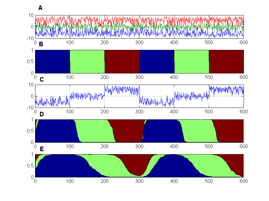
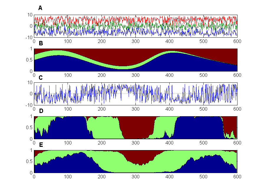
Figure 1: The stages of numerical experiments and the results of experts’ aggregation for two data generation methods (Method 1 – left, Method 2 - right). (A) – realizations of the trajectories for the three data generating distributions; (B) – weights of the distributions assigned by the data generating method; (C) – sequence sampled from the distributions defined by Method 1 and Method 2; (D) – weights of the experts assigned online by the AA using the rule (33) and Fixed Share update; (E) – weights of the experts assigned online using the rule (36) and Fixed Share.

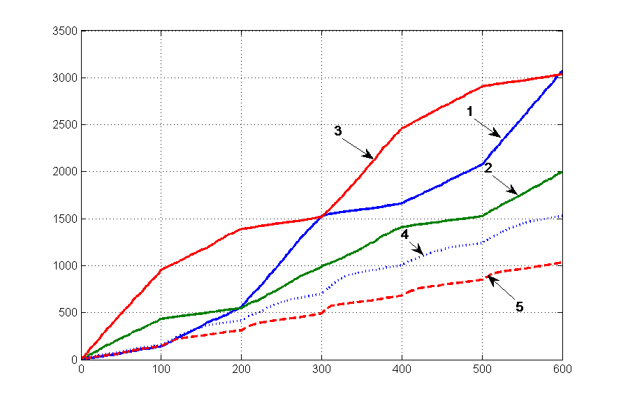
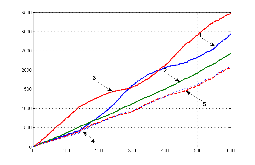
Figure 2: The cumulated losses of the experts (lines 1-3) and of the aggregating algorithm for both data generating methods (Method 1 – left, Method 2 - right) and for both methods of computing aggregated forecasts: line 4 – for the rule (35) and line 5 – for the rule (32). We note an advantage of rule (32) over rule (35) in the case of data generating Method 1, in which there is a rapid change in leadership of the data generating distributions.

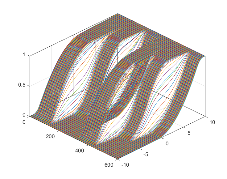
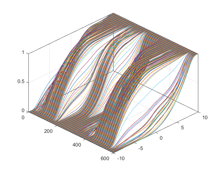
Figure 3: Empirical distribution functions obtained online as a result of aggregation of the distributions of three experts by the rule (32) for both data generating methods.

In this section we present the results of experiments with AA and WA which were performed on synthetic data. The initial data was obtained by sampling from a mixture of the three distinct probability distributions with the triangular densities. The time interval is made up of several segments of the same length, and the weights of the components of the mixture depend on time. We use two methods of mixing. By Method 1, only one generating probability distribution is a leader at each segment (i.e. its weight is equal to one). By Method 2, the weights of the mixture components vary smoothly over time (as shown in section B of Figure 1).

There are three experts $i=1,2,3$, each of which assumes that the time series under study is obtained as a result of sampling from the probability distribution with the fixed triangular density with given peak and base. Each expert evaluates the similarity of the testing point of the series with its distribution using ${\rm CRPS}$ score.

We compare two rules of aggregations of the experts’ forecasts: Vovk’s AA (32) and the weighted average WA (35).

Figure 1 shows the main stages of data generating (Method 1 – left, Method 2 - right) and the results of aggregation of the experts models. Section A of the figure shows the realizations of the trajectories of the three data generating distributions. The diagram in Section B displays the actual relative weights that were used for mixing of the probability distributions. Section C shows the result of sampling from the mixture distribution. The diagram of Sections D and E show the weights of the experts assigned by the corresponding Fixed Share algorithm in the online aggregating process using rules (32) and (35).

Figure 2 shows the cumulated losses of the experts and the cumulated losses of the aggregating algorithm for both data generating methods (Method 1 – left, Method 2 - right) and for both methods of computing the aggregated forecasts – by the rule (32) and by the rule (35). We note an advantage of rule (32) over the rule (35) in the case of data generating Method 1, in which there is a rapid change in leadership of the generating experts.

Figure 3 shows in 3D format the empirical distribution functions obtained online by Protocol 3 for both data generating methods and the rule (32).

5.2 Aggregation of probabilistic predictions with confidence

In Section 5.3 (below) we present results of numerical experiments with the real data and when prediction of the experts are supplied by the levels of confidence. In this case we use a modification of Protocol 3 – Protocol 3a, which is presented below.

Protocol 3a

  

Define $w_{i,1}=\frac{1}{N}$ for $1\leq i\leq N$.

FOR $t=1,\dots,T$

1. Receive the expert predictions – the probability distribution functions $F_{i,t}(u)$ and confidence levels $p_{i,t}$, where $1\leq i\leq N$.

2. Present the learner forecast – the probability distribution function $F_{t}(u)$ which is defined by the rule (32) (AA) or by the rule (35) (WA), where $w^{*}_{i,t}=\frac{p_{i,t}w_{i,t}}{\sum_{j=1}^{N}p_{j,t}w_{j,t}}$.

3. Observe the true outcome $y_{t}$ and compute the score ${\rm CRPS}(F_{i,t},y_{t})$ for the experts $1\leq i\leq N$ and the score ${\rm CRPS}(F_{t},y_{t})$ for the learner.

4. Update the weights of the (virtual) experts $1\leq i\leq N$

   $$w_{i,t+1}=w_{i,t}e^{-\eta(p_{i,t}{\rm CRPS}(F_{i,t},y_{t})+(1-p_{i,t}){\rm CRPS}(F_{t},y_{t}))},$$ (37)

   where $\eta=\frac{2}{b-a}$ if the rule (32) is used and $\eta=\frac{1}{2(b-a)}$ for the rule (35).

ENDFOR   

The performance of this algorithm is presented by the inequality (16) from Theorem 1, where $h_{t}={\rm CRPS}(F_{t},y_{t})$, $l_{i,t}={\rm CRPS}(F_{i,t},y_{t})$ and $\eta=\frac{2}{b-a}$ if the rule (32) for computing the learner’s forecast was used and $\eta=\frac{1}{2(b-a)}$ if the rule (35) was used.

5.3 Probabilistic forecasting of electrical loads

The second group of numerical experiments on probabilistic forecasting were performed with the data of the 2014 (GEFCOM 2014,Track Load) competition conducted on the Kaggle platform (Tao Hong et al. 2016).

The main unit of the training sample includes data on hourly electrical load for 69 months from January 2005 to September 2010 and data on hourly temperature measurements during 117 month period. Databases are available at http://www.kaggle.com/datasets.

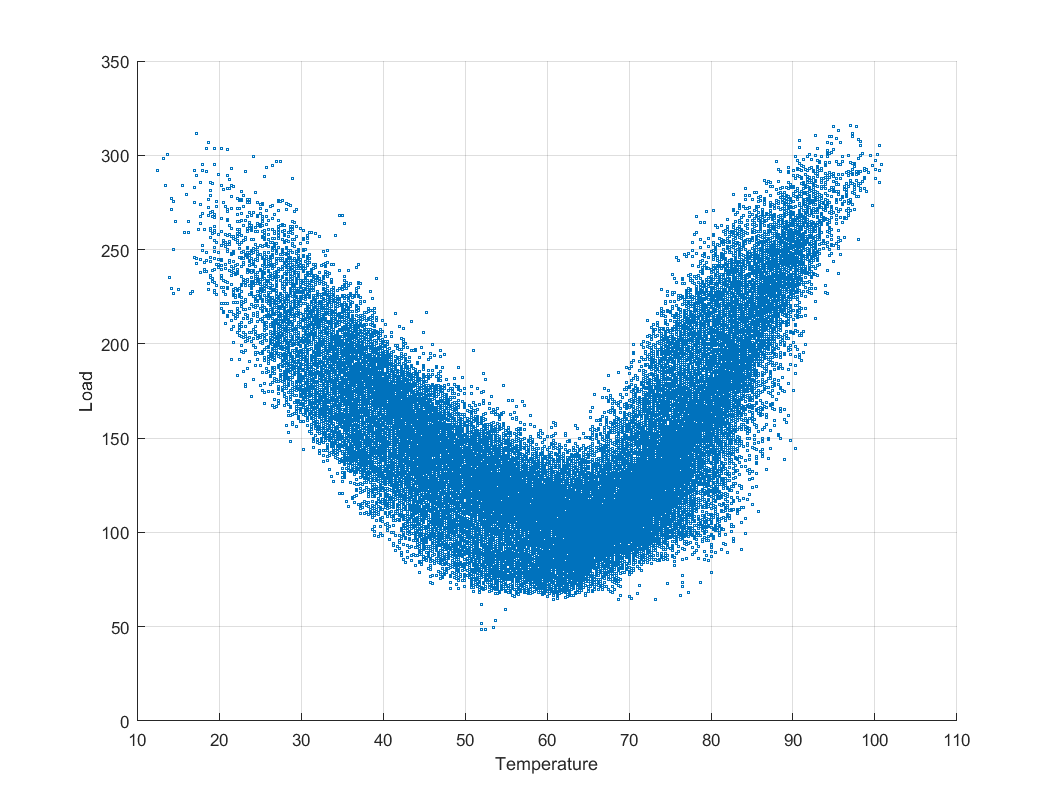
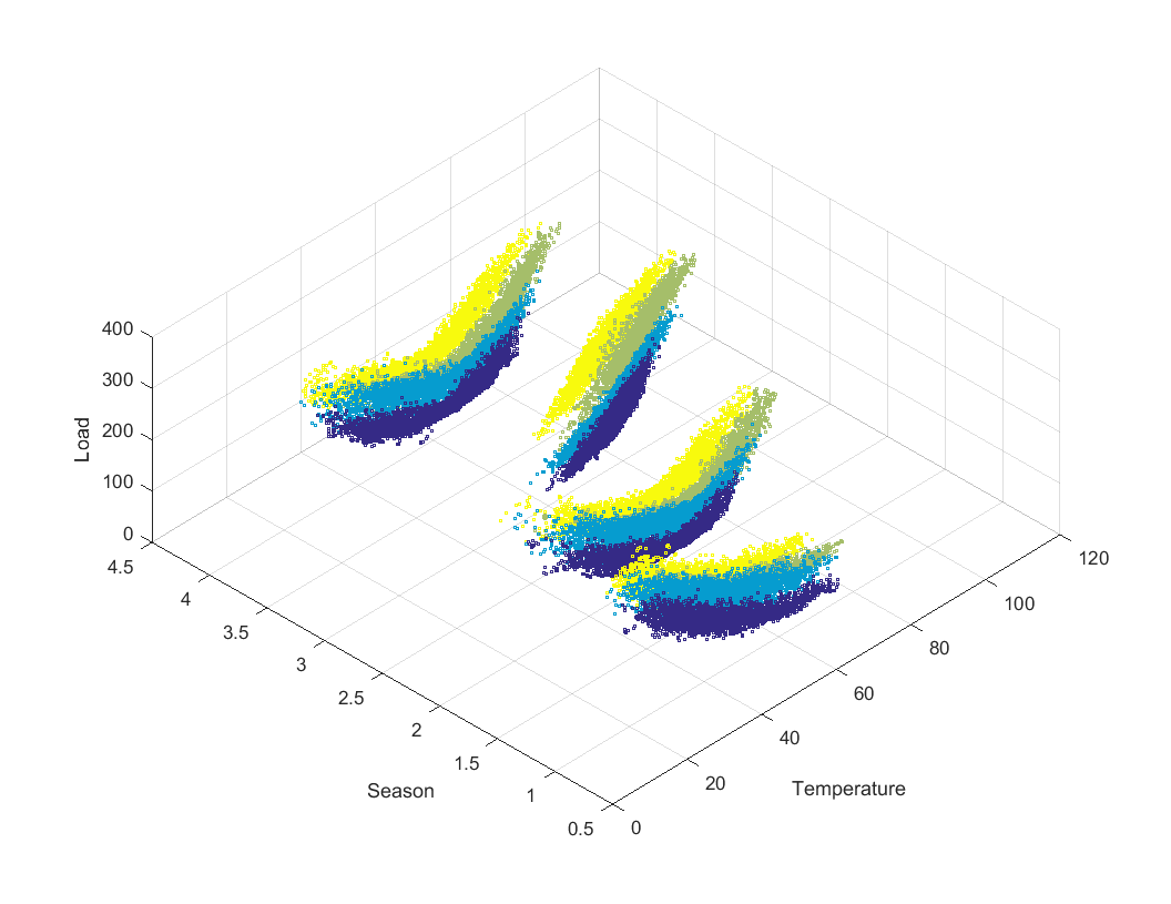
Figure 4: Daily temperature and electrical load paths for all days from January 2001 to September 2010. Left figure – all data; right figure – data grouped by seasons (Winter, Spring, Summer, Autumn) and time of day marked in color (Night, Morning, Day, Evening).

The scatter diagrams “Load - Temperature” for several sets of calendar parameters: (four seasons of the year and four consecutive intervals of day, each for 6 hours) are presented in Figure 4. The diagrams are constructed according to the training part of the sample.

Figure 4 shows the nature of the relationship between potential predictors and response. This data shows the dependence of electrical loads on temperature looking differently during different seasons and time of day. For each of the scattering diagrams presented, two temperature intervals can be distinguished in such a way that within each intervals the point cloud has a simple ellipsoidal shape. This provides the basis for using a mixture of normal distributions for the probabilistic forecast of the expected electrical load according to the short-term temperature forecast.

Scatter patterns on Figure 4 can serve as the basis for determining the pool of the experts. Each of them learns (builds a predictive probabilistic model) at sample points related to a predefined calendar segment, for example “Winter$\&$Morning”, etc. These segments should cover all possible combinations of calendar indicators present in the data.

A set of 21 specialized experts is defined by dividing the calendar space into areas where the relationship between temperature and electrical load can be described by a simple and relatively uniform dependence. To define an expert a combined sample of historical data consisting of the initial sample of “temperatures – loads” ensemble, as well as its competence area (season, time of day), was determined.

The anytime Expert 1 corresponds to the left part of Figure 4, Experts 2-5 correspond to four seasons (see right part of Figure 4). Experts 6-21 correspond to the colored parts of the plots on the right part of Figure 4. To construct the probability distribution of any expert, we use the method of Gauss Mixture Models (GMM), which is applied to the corresponding ensemble of “temperatures – loads”. This probabilistic model is presented as a mixture of two normal distributions.

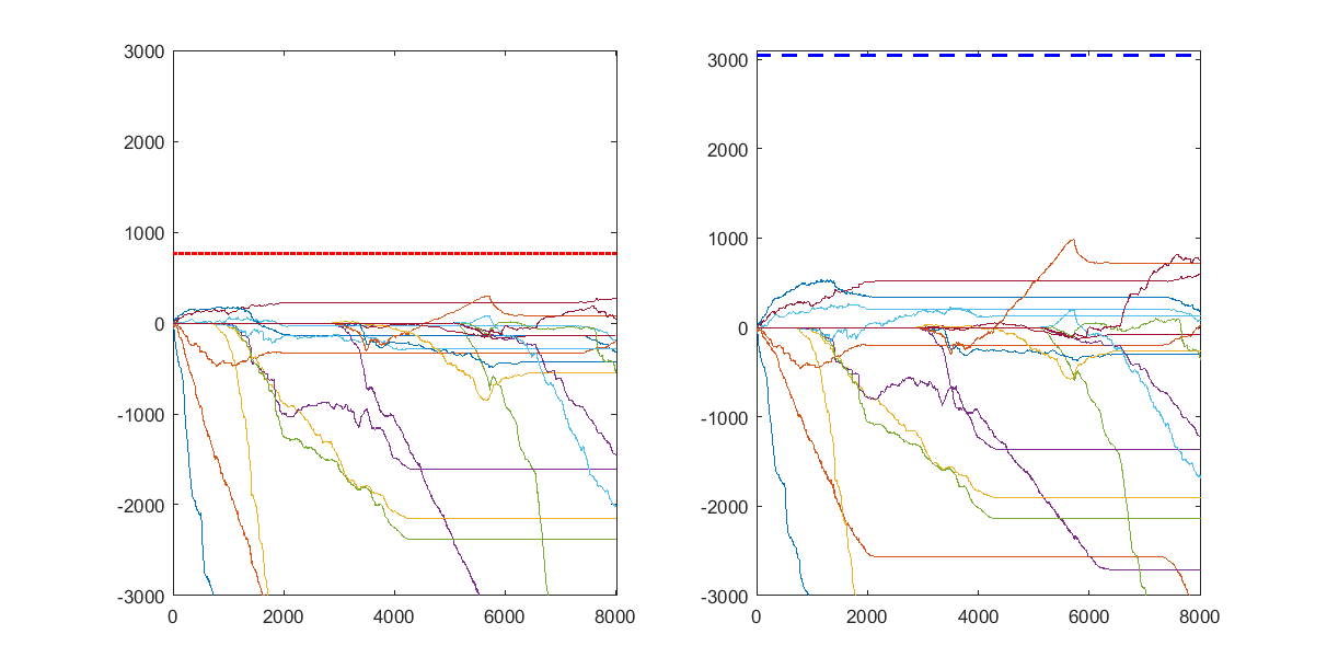
Figure 5: Discounted regret curves for AA (left) and WA (right) with respect to each of 21 specialized experts. The dotted lines above represents the theoretical bounds for the regret.

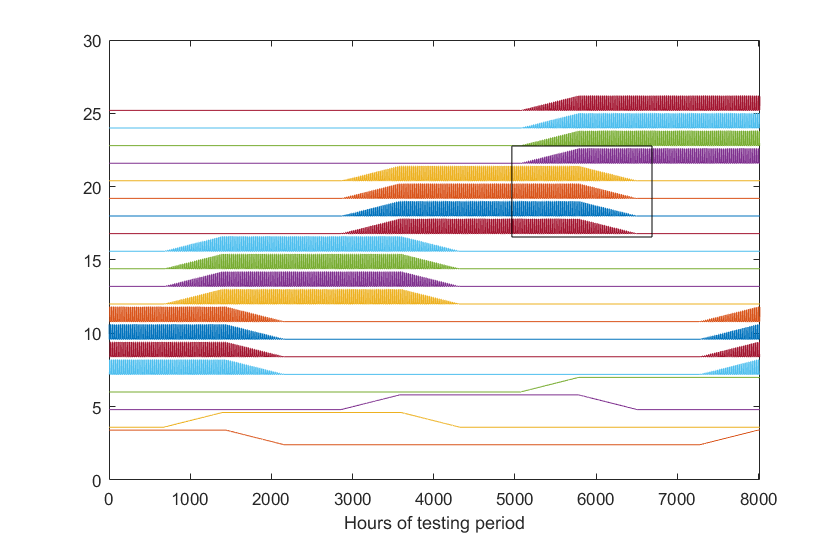
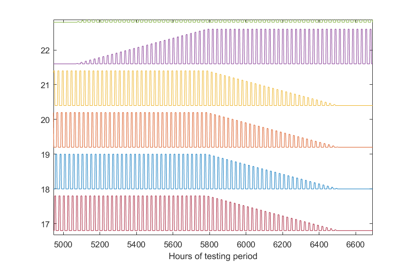
Figure 6: Left part: confidence levels for for Experts 2-5 (season experts) and 6–21 (“season$\&$time of day”). Right part: enlarged fragment.

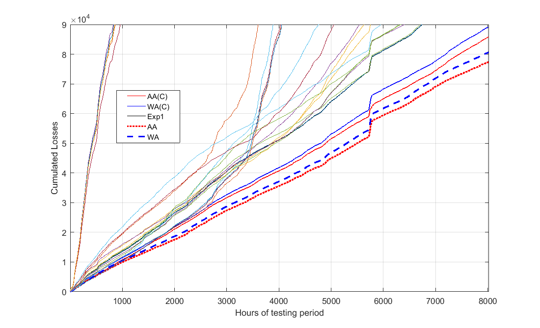
Figure 7: Comparative study of learning with/without specialization of the experts. 1) Cumulated losses of all 21 specialized experts working any time; 2) results of their aggregation by AA and WA, where confidence levels of the experts are set to 1; 3) results of aggregation by AA and WA of specialized experts, where theirs confidence levels are taken into account.

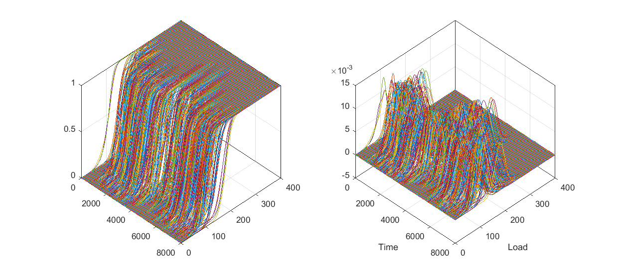
Figure 8: Time changing of probability forecasts – probability distribution functions (left) and of the corresponding densities (right).

We consider a particular forecasting problem – the short-term forecasting of a probability distribution function for one hour in advance. The scope of each expert is determined by its confidence function. When forecasting, the expert s smooth areas of competence are chosen wider than those areas in which this expert was trained. Thus, each expert competes with other experts working at overlapping intervals using the corresponding algorithm for combining experts with confidence levels from Section 5.2, like it was done for computing the pointwise forecasts by V yugin and Trunov (2019).

The discounted regret curves $T\to\sum\limits_{t=1}^{T}p_{i,t}(h_{t}-l_{i,t})$ for AA and WA with respect to each of 21 specialized experts are presented in Figure 5. The dotted lines above represent the theoretical bounds for the regret (see the inequality (16)).

To justify the role of confidence parameters, the comparative experiments were conducted. During the first experiment, all confidence values for each expert were equal to 1. In the second experiment, AA and WA algorithms used the experts predictions within the levels of their confidence.

The results of both experiments are presented in Figure 7. The cumulated losses of all 21 specialized experts working any time are presented in this figure. Cumulative loss curves show that specialized experts, which were trained only for certain types of data, quickly lose their effectiveness in other types of data areas and generally suffer large losses. An exception is Expert 1, who trained on all types of data.

The results of two methods of aggregation of these experts by AA and WA are also presented in Figure 7. In the first method of aggregation, confidence levels of all experts were equal to 1.

In the second method, algorithms AA and WA use specialized experts, where theirs confidence levels are set externally. They correspond to the training intervals of specialized experts, but are somewhat wider and monotonically decrease to zero outside these intervals (see example in Figure 6). Confidence levels were not optimized in this experiment. The results of aggregation by AA and WA of specialized experts are also presented in Figure 7. The results of the experiments show that the use confidence levels of specialized experts increases the efficiency of the process of online adaptation. These results also show that AA in all experiments slightly outperforms WA.

Time changes of probability forecasts (probability distribution functions) and of the corresponding densities are presented on Figure 8.

6 Conclusion

In this paper the problem of aggregating the probabilistic forecasts is considered. In this case, a popular example of proper scoring rule for continuous outcomes is the continuous ranked probability score ${\rm CRPS}$.

We present the theoretical analysis of the continuous ranked probability score ${\rm CRPS}$ in the prediction with expert advice framework and illustrate these results with computer experiments.

We have proved that the ${\rm CRPS}$ loss function is mixable and and then all machinery of the aggregating algorithm by Vovk (1998) can be applied. The proof is an application of prediction of packs by Adamskiy et al. (2017): the probability distribution function can be approximated by a piecewise-constant function and further the method of aggregation of the generalized square loss function have been used.

Basing on mixability of ${\rm CRPS}$, we propose two methods for calculating the predictions using the aggregating algorithm (AA) and the weighted average of forecasts of the experts (WA). The time-independent upper bounds for the regret were obtained for both methods.

The proposed methods are closely related to the so called ensemble forecasting (Thorey et al. 2017). In practice, the output of physical process models usually not probabilities, but rather ensembles. Ensemble forecasts are based on a set of physical models. Each model may have its own physical formulation, numerical formulation and input data. An ensemble is a collection of model trajectories, generated using different initial conditions of model equations. Consequently, the individual ensemble members represent likely scenarios of the future physical system development, consistent with the currently available incomplete information. In this case, the aggregation methods of the corresponding ensemble based probability distribution functions may be useful.

We have presented the results of numerical experiments based on the proposed methods and algorithms. These results show that two methods of computing forecasts AA and WA lead to similar empirical cumulative losses while the rule (32) results in four times less regret bound than (35). We note a significantly best performance of method AA (32) over method WA (35) in the case where there is a rapid change in leadership of the experts. This difference has been demonstrated in numerical experiments.

References

- Adamskiy et al. (2017) D. Adamskiy, T. Bellotti, R. Dzhamtyrova, Y. Kalnishkan. Aggregating Algorithm for Prediction of Packs. Machine Learning, https://link.springer.com/article/10.1007/s10994-018-5769-2 (arXiv:1710.08114 [cs.LG]).
- Blum and Mansour (2007) A. Blum, Y. Mansour. From external to internal regret. Journal of Machine Learning Research. 8:1307–1324, 2007.
- Brier (1950) G.W. Brier. Verification of forecasts expressed in terms of probabilities. Mon. Weather Rev., 78: 1–3, 1950.
- Bröcker et al. (2007) J. Bröcker, L.A. Smith. Scoring probabilistic forecasts: The importance of being proper. Weather and Forecasting, 22: 382–388, 2007.
- Bröcker et al. (2008) J. Bröcker, L.A. Smith. From ensemble forecasts to predictive distribution functions. Tellus A, 60: 663–678, 2008.
- Bröcker (2012) J. Bröcker. Evaluating raw ensembles with the continuous ranked probability score. Q. J. R. Meteorol. Soc., 138: 1611–1617, July 2012 B.
- Chernov and Vovk (2009) A. Chernov and V. Vovk. Prediction with expert evaluators advice. In Algorithmic Learning Theory, ALT 2009, Proceedings, volume 5809 of LNCS, pages 8- 22. Springer, 2009.
- Cesa-Bianchi and Lugosi (2006) N. Cesa-Bianchi, G. Lugosi. Prediction, Learning, and Games, Cambridge University Press, 2006.
- Cesa-Bianchi et al. (2007) N. Cesa-Bianchi, Y. Mansour, and G. Stoltz. Improved second-order bounds for prediction with expert advice. Machine Learning. 66(2/3):321–352, 2007.
- Devaine et al. (2013) M. Devaine, P. Gaillard, Y. Goude, G. Stoltz. Forecasting electricity consumption by aggregating specialized experts. Machine Learning. 90(2): 231–260, 2013.
- Epstein (1969) E.S. Epstein. A scoring system for probability forecasts of ranked categories. J. Appl. Meteorol. Climatol., 8: 985–987, 1969.
- Freund and Schapire (1997) Y. Freund, R.E. Schapire. A Decision-Theoretic Generalization of On-Line Learning and an Application to Boosting. Journal of Computer and System Sciences, 55: 119–139, 1997.
- Freund et al. (1997) Y. Freund, R.E. Schapire, Y. Singer, M.K. Warmuth. Using and combining predictors that specialize. In: Proc. 29th Annual ACM Symposium on Theory of Computing. 334–343, 1997.
- Herbster and Warmuth (1998) M. Herbster, M. Warmuth. Tracking the best expert. Machine Learning, 32(2): 151–178, 1998.
- Jordan et al. (2018) A. Jordan, F. Krüger, S. Lerch. Evaluating Probabilistic Forecasts with scoring Rules, arXiv:1709.04743
- Kalnishkan et al. (2015) Y. Kalnishkan, D. Adamskiy, A. Chernov, T. Scarfe. Specialist Experts for Prediction with Side Information. IEEE International Conference on Data Mining Workshop (ICDMW). IEEE, 1470–1477, 2015.
- Korotin et al. (2019) A. Korotin, V. V’yugin, E. Burnaev. Integral Mixabilty: a Tool for Efficient Online Aggregation of Functional and Probabilistic Forecasts. arXiv:1912.07048 [cs.LG], 2019 https://arxiv.org/abs/1912.07048
- Littlestone and Warmuth (1994) N. Littlestone, M. Warmuth. The weighted majority algorithm. Information and Computation, 108: 212–261, 1994.
- Matheson and Winkler (1976) J.E. Matheson, R.L. Winkler. Scoring Rules for Continuous Probability Distributions. Management Science, 22(10): 1087- 1096, 1976. doi:10.1287/mnsc.22.10.1087
- Raftery et al. (2005) A.E. Raftery, T. Gneiting, F. Balabdaoui, M. Polakowski. Using Bayesian model averaging to calibrate forecast ensembles. Mon. Weather Rev., 133: 1155–1174, 2005.
- Tao Hong et al. (2016) Tao Hong,, Pierre Pinson, Shu Fanc, Hamidreza Zareipour, Alberto Troccoli, Rob J. Hyndman. Probabilistic energy forecasting: Global Energy Forecasting Competition 2014 and beyond. International Journal of Forecasting 32: 896- 913, 2016.
- Thorey et al. (2017) J. Thorey, V. Mallet and P. Baudin. Online learning with the Continuous Ranked Probability Score for ensemble forecasting. Quarterly Journal of the Royal Meteorological Society, 143: 521- 529, January 2017 A DOI:10.1002/qj.2940
- Vovk (1990) V. Vovk, Aggregating strategies. In M. Fulk and J. Case, editors, Proceedings of the 3rd Annual Workshop on Computational Learning Theory, 371–383. San Mateo, CA, Morgan Kaufmann, 1990.
- Vovk (1998) V. Vovk, A game of prediction with expert advice. Journal of Computer and System Sciences, 56(2): 153–173, 1998.
- Vovk (2001) V. Vovk. Competitive on-line statistics. International Statistical Review, 69: 213–248, 2001.
- Vovk et al. (2019) V. Vovk, J. Shen, V. Manokhin, Min-ge Xie. Nonparametric predictive distributions based on conformal prediction. Machine Learning, 108(3): 445- 474, 2019. https://doi.org/10.1007/s10994-018-5755-8
- V yugin and Trunov (2019) V. V’yugin, V. Trunov. Online aggregation of unbounded losses using shifting experts with confidence. Machine Learning, 108(3): 425–444, 2019. https://doi.org/10.1007/s10994-018-5751-z
- V yugin and Trunov (2019) V. V’yugin, V. Trunov. Online Learning with Continuous Ranked Probability Score, Proceedings of Machine Learning Research 105: 163–177, 2019.