SAFE ML: Surrogate Assisted Feature Extraction for Model Learning

Abstract

Complex black-box predictive models may have high accuracy, but opacity causes problems like lack of trust, lack of stability, sensitivity to concept drift. On the other hand, interpretable models require more work related to feature engineering, which is very time consuming. Can we train interpretable and accurate models, without timeless feature engineering? In this article, we show a method that uses elastic black-boxes as surrogate models to create a simpler, less opaque, yet still accurate and interpretable glass-box models. New models are created on newly engineered features extracted/learned with the help of a surrogate model. We show applications of this method for model level explanations and possible extensions for instance level explanations. We also present an example implementation in Python and benchmark this method on a number of tabular data sets.

1 Motivation

Questions of trust in machine learning models became crucial issues in recent years. Complex predictive models have various applications in different areas Paliwal and Kumar (2009); Kourou et al. (2015) and an increasing number of people use machine learning solutions in everyday life. Hence, it is important to ensure that predictions of these models are reliable. There are four requirements whose fulfillment is essential to ensure that predictive model is trustworthy and accessible: (1) high model performance, (2) auditability, (3) interpretability, and (4) automaticity.

(1) High model performance means that a model rarely makes wrong predictions or the prediction error is small on average. Usually, this can be achieved by using complex, so-called black-box models, such as, boosting trees Chen and Guestrin (2016) or deep neutral networks Goodfellow et al. (2016). The opposite of black-boxes are glass-boxes. They are simple, interpretable models, such as linear regression, logistic regression, decision trees, regression trees, and decision rules.

Model performance ensures only a part of information about model’s quality. Model’s (2) auditability guarantees that the model can be verified with respect to different criteria. They are, for example, stability, fairness, and sensitivity to a concept drift. There are tools that allow to audit black-box models Gosiewska and Biecek (2018), yet simple glass-boxes offer more extended range of diagnostic methods Harrell (2006).

The third requirement is an (3) interpretability, which became an important topic in recent years O’Neil (2016). Machine learning models influence people’s lives, in particular, they are used by financial, medical, and security institutions. Models have an impact on whether we get a loan Huang et al. (2007), what type of treatment we receive Cruz and Wishart (2006), or even whether we are searched by the police Nath (2006). Therefore, models reasoning should be transparent and accessible. There is an ongoing debate about the right to explanation, what does it mean and how it can be achieved Wachter et al. (2017); Edwards and Veale (2018).

The (4) automaticity of machine learning methods is spreading rapidly. Due to the increasing computational power, it becomes easier and easier to obtain more precise models, usually in an automatic manner. There are automated frameworks for AutoML like autokeras, auto-sklearn, TPOT Jin et al. (2018); Feurer et al. (2015); Olson et al. (2016) that allow one to train a model even without any statistical knowledge or even programming skills. Yet, machine learning specialists can also take an advantage of automated methods of modeling. Such methods reduce time needed to train the model, therefore human effort can be directed towards more creative and sophisticated tasks than testing wide range of parameters and models.

People usually choose automatically fitted black-box models that achieve high performance at the cost of auditability and interpretability. As a response to this problem, the methodology for explaining predictions of black-box models, so called post-hoc interpretability, is under active development. There are several approaches to explaining the global behavior of black-boxes. Model can be reduced to simple if-then rules Puri et al. (2017) or decision trees Hall (2018). However, these explanations are simplifications of models and may be inaccurate. As a consequence, they may be misleading or even harmful. Hence, in many applications it is better to train a transparent, interpretable model than apply explanations to a complex model Tan et al. (2017); Rudin (2018). Therefore, automated methods of obtaining interpretable models, while maintaining the predictive capabilities of a complex model, are extremely important.

In this article, we present a method for Surrogate Assisted Feature Extraction for Model Learning (SAFE ML). This method uses a surrogate model to assist feature engineering and lead to training accurate and transparent glass-box model. In this approach, surrogate model should be accurate to produce best feature transformation, yet it does not have to be interpretable. Based on the new features, the transparent glass-box model is trained. In many cases the high accuracy of black-box models comes from good data representation and this is something than can be next extracted from the model.

The SAFE ML method is flexible and model agnostic, any class of models may be used as a surrogate model and as a glass-box model. Therefore, surrogate model may be selected to fit the data as best as possible, while glass-box model one can be selected according to the particular task or abilities of the end-users to interpreting models.

An advantage of this methodology is that the final glass-box model has a performance close to the surrogate model. By changing the representation of the data, SAFE ML allows to gain interpretability with minimal or no reduction of model performance.

The SAFE ML method can be used as a step in training a model with AutoML methods. We can use AutoML to fit elastic and complex model, then use SAFE to obtain a transparent model.

The paper is organized as follows. Section 2 provides a description of the SAFE algorithm. Section 3 contains illustrations and benchmarks for the SAFE method for regression and classification problems. Extensions for instance-level approaches and interactions are discussed in Section 4. Conclusions are in Section 5.

2 Description of the SAFE Algorithm

Figure 1: The SAFE ML algorithm in four steps, 1. train elastic surrogate model, 2. approximate model response, 3. extract transformations and new features, 4. train refined model.

The SAFE ML algorithm uses a complex model as a surrogate. New binary features are created on the basis of surrogate predictions. These new features are used to train a simple refined model.

Illustration of the SAFE ML method is presented in Figure 1. In the Algorithm 1 we describe how data transformations are extracted from the surrogate model while in Algorithm 2 we show how to train a new refined model based on transformed features. Below, we explain details of the terminology being used in algorithms. Let $x_{1},x_{2},...,x_{p}$ be features in the surrogate model $M$. A subset of all features except $x_{i}$ we denote as $x_{-i}$.

The partial dependence profile Friedman (2001) is defined as

$$f_{i}(x_{i})=\mathbb{E}_{x_{-i}}[M(x_{i},x_{-i})],$$

and calculated as

$$\hat{f}_{i}(x_{i})=\frac{1}{n}\sum_{j=1}^{n}M(x_{i}^{j},x_{-i}^{j}),$$

where $n$ is the number of observations and $x_{i}^{j}$ is a value of the $i$-th feature for the $j$-th instance. Partial dependence function describes the expected output condition on a selected variable. The visualization of this function is Partial Dependence Plot Greenwell (2017), an example plot is presented in Step 1 in Figure 1.

The change point method Truong et al. (2018) is used to identify times when the probability distribution of a time series changes. The hierarchical clustering Rokach and Maimon (2005) is an algorithm that groups observations into clusters. It involves creating a hierarchy of clusters that have a predetermined ordering. Step 2 in Figure 1 corresponds to both change point method and hierarchical clustering.

Algorithm 1 Surrogate Assisted Feature Extraction

  Input: data $X_{n\times p}$, surrogate model $M$, regularization penalty $\lambda$.

  Start:

  for $i=1$ to $p$ do

     Let $x_{i}$ be $i$-th feature.

     if $x_{i}$ is numerical then

        Calculate partial dependence profile $f_{i}(x)$ for feature $x_{i}$.

        Approximate $f_{i}(x)$ with interpretable features $x^{*}_{i}$, for example, use the change point method to discretize the variable with regularization penalty $\lambda_{i}$.

        Save transformation $t_{i}(x)$ that transforms $x_{i}$ into $x_{i}^{*}$.

     end if

     if $x_{i}$ is categorical then

        Calculate model responses for each observation with imputed each possible value of $x_{i}$.

        Merge levels of $f_{i}(x)$ with similar model responses, for example use the hierarchical clustering with number of clusters $\lambda_{i}$.

        Save transformation $t_{i}(x)$ that transforms $x_{i}$ into $x_{i}^{*}$.

     end if

  end for

  Sets of transformations $T^{*}=\{t_{1},...,t_{p}\}$ may be used to create new data $X^{*}$ from features $x_{i}^{*}=t_{i}(x_{i})$.

Algorithm 2 Model Learning with Surrogate Assisted Feature Extraction

  Input: data $X^{new}_{m\times p}$, set of transformations $T^{*}$ derived from surrogate model $M$.

  Start:

  Transform dataset $X$ into $X^{*,new}=T^{*}(X^{new})$.

  Create transparent model $M^{new}$ based on $X^{*,new}$.

3 Application and Benchmarks

In this section, we perform SAFE ML on selected data sets for regression and classification problems. A summary discussion of the results is conducted at the end of this section.

Examples are generated with scikit-learn models Pedregosa et al. (2011) and SafeTransformer. SafeTransformer is a Python library that implements SAFE ML method.

Code that generates artificial data sets and performs SAFE ML method and can be found in the GitHub repository: https://github.com/agosiewska/SAFE_examples.

3.1 Classification - Artificial Data Set

We compare performance of naïve logistic regression, surrogate xgboost, and refined logistic regression. Here naïve regression means that we fill vanilla regression model without any feature engineering.

This example is performed on the artificial data set SIMULD2 for binary classification. SIMULD2 consists of 500 observations and three variables. Variable $y$ is a binary target. Variable $X1$ is continuous, uniform distributed at range from $-5$ to $5$ with normally distributed noise. Variable $X2$ is categorical with 40 levels.

As can be seen in Table 1, refined logistic regression performs better than the other two models. Refined logistic regression achieves even better accuracy and AUC than xgboost model, while being a more transparent model.

It may be surprising that the refined model is better than the surrogate one, however there are some reasons for that. Elastic models are better to capture non-linear relations but at the price of larger variance for parameter estimation. In some cases the refined models will work on better features and will have less parameters to train, thus it can outperform the surrogate model.

Table 1: Results of the SAFE method for models trained on the SIMULD2 data set. SAFE was performed with penalty equals $0.42625$.

Model	Accuracy	AUC
Naïve logistic regression	0.736	0.897
Surrogate xgboost	0.960	0.982
Refined logistic regression	0.976	0.989

Partial Dependence Plot in Figure 2 shows the relationship between variable $X1$ and output of the xgboost model. This pattern is close to real association, which is a step function with discontinuities in $-3$ and $2.5$. This relationship could not be caught by logistic regression. However, in Figure 2, we can see that SAFE ML method divided $X1$ variable into three binary variables. This make it possible for refined logistic regression to capture the non-linearity.

Variable $X2$ consists of 40 levels, yet process of generating target variable y distinguishes between variables in three groups. When examining how SAFE ML has grouped variables, one can see that groups almost match up with real dependencies. This caused that instead of one variable of 40 levels, the new model was trained on 3 binary variables. This means that transformed features better reflected the real relationships.

Figure 2: An expected response of the xgboost model conditioned on the variable X1. Black vertical lines marks points of the discretization calculated with SAFE ML.

3.2 Regression - Boston Housing

Second example is performed on Boston Housing data set Harrison and Rubinfeld (1978). Boston Housing consists of 506 rows and 14 columns. The target variable is medv (median value of owner-occupied homes).

We compare performances of naïve linear regression, surrogate xgboost, and refined linear regression.

As described in Section 2, feature extraction in SAFE ML algorithm depends on a choice of a regularization penalty $\lambda$. Figure 3 shows performances of models as functions of penalty. Mean Square Errors (MSE) of the refined linear regression models are, in general, close to MSE of surrogate model. Thus, the use of a simpler model did not negatively affect the performance. At the same time, we gained transparency.

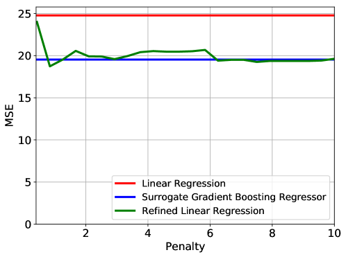
Figure 3: Dependence between SAFE ML method’s penalty and MSE for refined model.

Partial Dependence Plot for xgboost model and variable ZN is presented in Figure 4. Flexible boosting model captured the non-linear relationship between variable ZN and target medv. As a result, SAFE ML method divided ZN variable into two binary features to improve performance of refined model.

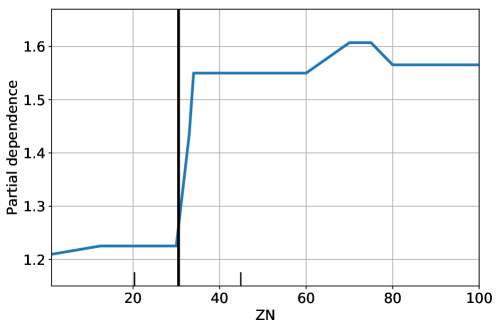
Figure 4: Partial Dependence Plot (PDP) of the gradient boosting model and ZN variable . Black vertical line indicates variable split generated with SAFE ML method.

3.3 Benchmark on a Number of Tabular Data Sets

In this section we benchmark the SAFE ML method on a number of tabular data sets for regression and classification problems. We compare performances of three groups of models: simple models trained without SAFE ML feature transformation, complex surrogate models, and refined interpretable models.

3.3.1 Benchmark for Classification

We train classification models on six different data sets. They are two simulated data sets, Titanic from Kaggle, Blood Transfusion Service Center Yeh et al. (2009), Teaching Assistant Evaluation form UCI Machine Learning Repository Dheeru and Karra Taniskidou (2017), and Pima Indian Diabetes Johannes (1988).

We use Accuracy and AUC metrics to evaluate models. Logistic regression and classification trees trained without any feature extraction are baselines. Complex xgboost models are surrogates required to perform SAFE ML algorithm. Parameters of surrogate models differ between data sets. Refined models are logistic regression models and classification trees. To chose best penalty for SAFE ML transformations, for each surrogate model we examined 25 equally spaced penalties in the range from $0.01$ to $10$. The criterion was performance of a refined model.

Results of benchmarking are in Table 2. For 22 out of 24 cases, refined model surpasses baseline model. In more than half cases, refined model outperforms baseline and surrogate model.

Table 2: Performances of models trained on six data sets for classification. Artificial data sets are marked by (A). Headers indicate class of baseline model (BASE.) and refined model (REF.). In each case, surrogate model (SURR.) is xgboost.

Logistic Regression - AUC
Data set	BASE.	SURR.	REF.
SIMULD1 (A)	0.833	0.980	0.963
SIMULD2 (A)	0.897	0.982	0.989
Titanic	0.861	0.896	0.870
Blood Transfusion	0.670	0.679	0.668
Teaching Evaluation	0.725	0.838	0.821
Pima Indian Diabetes	0.814	0.822	0.838
Logistic Regression - Accuracy
Data set	BASE.	SURR.	REF.
SIMULD1 (A)	0.744	0.888	0.912
SIMULD2 (A)	0.736	0.960	0.976
Titanic	0.798	0.834	0.834
Blood Transfusion	0.749	0.754	0.668
Teaching Evaluation	0.842	0.842	0.868
Pima Indian Diabetes	0.745	0.734	0.771
Classification Tree - AUC
Data set	BASE.	SURR.	REF.
SIMULD1 (A)	0.877	0.980	0.972
SIMULD2 (A)	0.928	0 982	0.983
Titanic	0.777	0.896	0.878
Blood Transfusion	0.598	0.667	0.683
Teaching Evaluation	0.763	0.817	0.842
Pima Indian Diabetes	0.665	0.822	0.767
Classification Tree - Accuracy
Data set	BASE.	SURR.	REF.
SIMULD1 (A)	0.896	0.888	0.912
SIMULD2 (A)	0.928	0.96	0.976
Titanic	0.794	0.834	0.839
Blood Transfusion	0.738	0.775	0.759
Teaching Evaluation	0.842	0.842	0.895
Pima Indian Diabetes	0.688	0.734	0.760

3.3.2 Benchmark for regression

In this section, we examine performance of the SAFE ML method on 5 data sets for regression problems. They are Energy Efficiency and Yacht Hydrodynamics form UCI Machine Learning Repository Dheeru and Karra Taniskidou (2017), Boston Housing Harrison and Rubinfeld (1978), Warsaw Apartments Biecek (2018), and Real Estates Yeh and Hsu (2018).

Base and refined models are linear regression models. We use xgboosts as a surrogate model, xgboost parameters differ between data sets. To chose best penalty for SAFE ML transformations we examine 25 equally spaced penalties in the range from $0.01$ to $10$ and MSE criterion.

Results are presented in Table 3. For all data sets, baseline models outperform base models. For 3 out of 5 data sets, refined linear model achieves better performance than xgboost model.

Table 3: Performances of models trained on five data sets for regression problem. Artificial data sets are marked by (A). Baseline models (BASE.) and refined models (REF.) are linear regression models. Surrogate models (SURR.) are xgboost models. Performance metric is MSE, values in columns are scaled to MSE for baseline model.

Data set	BASE.	SURR.	REF.
Warsaw Apartments (A)	1	7.12	64.99
Real Estates	1	1.02	1.38
Boston Housing	1	1.27	1.32
Energy efficiency	1	43.09	8.88
Yacht Hydrodynamics	1	267.75	105.17

3.4 Benchmark Summary

We examined 6 data sets for regression and 5 data sets for classification. In more than half of the cases, refined model had outperformed surrogate model. In majority of the rest examples performance differences between surrogate and refined models were minimal.

Refined models are simple, with a small number of parameters, therefore one could conclude that refined models generalize data better than complex models. However, it is worth noting that the refined models generalize relationships that were captured by surrogate models. Thus, without a complex model as a surrogate, it would not have been possible. With SAFE ML method, transferring knowledge about relationships to a simple model is automatic and do not require detailed investigation of the complex model.

Even if black-box model gains better results, it is still worth considering applying transparent glass-box model. As we have seen in previous examples, performance of surrogate and refined model were, in general, close to each other. The advantage of a simpler model is that we gain transparency, interpretability and auditability.

4 Future extensions of the SAFE ML method

4.1 Instance Level Problems

In previous sections, we showed how to use complex surrogate models to extract global, interpretable features. SAFE ML method could be also extended to instance level feature extraction. A complex model can capture local relationships between variables. Therefore, we may consider several local, interpretable models, instead of one global model.

There are several approaches to obtain locality, we can subset data set, reweight original data, or simulate instances from the original data distribution. One of the examples of local model approximations is LIME (Local interpretable model-agnostic explanations) Ribeiro et al. (2016). It is a method for generating local models that approximate the predictions of the underlying complex model. Local models are simple, such as, LASSO regression. Since LASSO is a method for selecting variables, while applying LIME we perform also a feature extraction. However, this method is not capable of extracting new interpretable features.

An extension of the LIME that includes extraction of interpretable features is localModel (Local Explanations of Machine Learning Models for Tabular Data) Staniak and Biecek (2019). Local interpretable features are created by discretization of numerical features due to the splits of the decision tree. Categorical features are discretized by merging levels using the marginal relationship between the feature and the model response. Locality is obtained by generating a random number of interpretable inputs around the explained instance. Then, LASSO regression model is fitted to new features and original model’s responses.

The idea behind localModel is similiar to SAFE ML. However, localModel is used to make statements about predictions and behaviour of the underlying black-box model, while the idea of SAFE is to create new refined model to make its own predictions.

4.2 Interactions Extractions

SAFE ML algorithm is used for transforming single features. One can consider extending this approach of interactions. There are methods of capturing interactions from random forest Paluszynska and Biecek (2017) or xgboost Foster (2017). This can be used for extraction of new features which contain information about interactions between variables.

5 Discussion

In this article, we presented SAFE ML algorithm that uses surrogate model to feature transformations. New features are then used to train refined glass-box model.

We benchmarked SAFE ML for regression and classification problems. The results confirmed that SAFE ML algorithm produces features that can be further used to fit accurate and transparent model. We also justified the advantage of refined models over surrogate black-boxes.

We also discussed possible extensions of SAFE ML to instance level problems. In addition, we see the possibility of extending the SAFE ML method to include interaction extraction.

5.1 Benchmarking Methodology

Benchmarks in Section 3 were based on a single split into training and test data sets. In further research, benchmarks could include k-fold cross-validation technique. However, while applying cross-validation, it would be necessary to take into account values of penalty. In Section 3 we were selecting a penalty on the basis of the model performance on a test data. The use of cross-validation will cause that values of penalty for each fold will be different. Thus it will not be possible to point the best penalty.

5.2 Conclusions

The SAFE ML method allows us to fulfill four requirements of trustworthy predictive model, stated in Section 1. One can choose a final refined model, accordingly to the simplicity and transparency, therefore statement (3) about interpretability is accomplished. Simple models, such as, linear regression and logistic regression are extensively described from a mathematical point of view. As a result, there are many methods to diagnose such models. Therefore, requirement of the (2) auditability is also fulfilled. In Section 3 we showed that performances of refined models are close to performance of complex surrogate models. Therefore, SAFE ML method allows to gain (1) high model performance. In Section 3 we also argued that SAFE ML algorithm allows automatic feature transformation for the purpose of fitting refined model. This approach allows you to omit examining a complex model. Thus (4) automaticity is also accomplished.

5.3 Similar Nomenclature

The phrase surrogate model is occasionally referred to an interpretable glass-box model that approximates predictions of a black-box model Hall et al. (2017). The surrogate model in this sense mimics most of the properties of the model under consideration, and is used to makes statements about the black-box model and not about the real world. However, there is no unambiguous nomenclature for this kind of problem. Models that mimic black-boxes are called also proxy models, shadow models, metamodels, response surface models, emulators Molnar (2018); Hall (2018).

Therefore, our meaning of the term surrogate model is not a duplication the meaning of the existing phrase. In this article, we refer surrogate model to a complex model that supports training interpretable model.

5.4 Software and Code

Benchmarks from Section 3 were generated with SafeTransformer Python library available at (https://github.com/olagacek/SAFE). Code that generates benchmarks is availible on Github: (https://github.com/agosiewska/SAFE_examples).

6 Acknowledgements

Alicja Gosiewska was financially supported by the grant of Polish Centre for Research and Development POIR.01.01.01-00-0328/17. Przemyslaw Biecek was financially supported by the grant NCN Opus grant 2017/27/B/ST6/01307.

References

- Biecek (2018) P. Biecek. DALEX: Explainers for Complex Predictive Models in R. Journal of Machine Learning Research, 19(84):1–5, 2018. URL http://jmlr.org/papers/v19/18-416.html.
- Chen and Guestrin (2016) T. Chen and C. Guestrin. XGBoost: A Scalable Tree Boosting System. 2016. URL http://arxiv.org/abs/1603.02754.
- Cruz and Wishart (2006) J. A. Cruz and D. S. Wishart. Applications of Machine Learning in Cancer Prediction and Prognosis. Cancer Informatics, 2, 2006. URL https://doi.org/10.1177/117693510600200030.
- Dheeru and Karra Taniskidou (2017) D. Dheeru and E. Karra Taniskidou. UCI Machine Learning Repository, 2017. URL http://archive.ics.uci.edu/ml.
- Edwards and Veale (2018) L. Edwards and M. Veale. Enslaving the Algorithm: From a “Right to an Explanation” to a “Right to Better Decisions”? IEEE Security and Privacy, 16(3):46–54, 2018. URL https://doi.org/10.1109/msp.2018.2701152.
- Feurer et al. (2015) M. Feurer, A. Klein, K. Eggensperger, J. Springenberg, M. Blum, and F. Hutter. Efficient and Robust Automated Machine Learning. In Advances in Neural Information Processing Systems 28, pages 2962–2970. 2015. URL https://bit.ly/2yQL2Dh.
- Foster (2017) D. Foster. xgboostExplainer: An R package that makes xgboost models fully interpretable, 2017. URL https://github.com/AppliedDataSciencePartners/xgboostExplainer/. R package version 0.1.
- Friedman (2001) J. H. Friedman. Greedy function approximation: A gradient boosting machine. Ann. Statist., 29(5):1189–1232, 10 2001. URL https://doi.org/10.1214/aos/1013203451.
- Goodfellow et al. (2016) I. Goodfellow, Y. Bengio, and A. Courville. Deep Learning. 2016. http://www.deeplearningbook.org.
- Gosiewska and Biecek (2018) A. Gosiewska and P. Biecek. auditor: an R Package for Model-Agnostic Visual Validation and Diagnostic. 2018. URL https://arxiv.org/abs/1809.07763.
- Greenwell (2017) B. M. Greenwell. pdp: An R Package for Constructing Partial Dependence Plots. The R Journal, 9(1):421–436, 2017. URL https://doi.org/10.32614/RJ-2017-016.
- Hall (2018) P. Hall. On the Art and Science of Machine Learning Explanations. In Proceedings of the JSM, Statistical Computing Section. Alexandria, VA: American Statistical Association, pages 1781–1799, 2018.
- Hall et al. (2017) P. Hall, N. Gill, M. Kurka, and W. Phan. Machine Learning Interpretability with H2O Driverless AI. 2017. URL: http://docs.h2o.ai/driverless-ai/latest-stable/docs/booklets/MLIBooklet.pdf.
- Harrell (2006) F. E. Harrell, Jr. Regression Modeling Strategies. Berlin, Heidelberg, 2006.
- Harrison and Rubinfeld (1978) D. Harrison and D. L. Rubinfeld. Hedonic housing prices and the demand for clean air. Journal of Environmental Economics and Management, 5(1):81–102, 1978. URL https://doi.org/10.1016/0095-0696(78)90006-2.
- Huang et al. (2007) C.-L. Huang, M.-C. Chen, and C.-J. Wang. Credit scoring with a data mining approach based on support vector machines. Expert Systems with Applications, 33(4):847–856, 2007. URL https://doi.org/10.1016/j.eswa.2006.07.007.
- Jin et al. (2018) H. Jin, Q. Song, and X. Hu. Auto-Keras: Efficient Neural Architecture Search with Network Morphism, 2018.
- Johannes (1988) R. S. Johannes. Using the ADAP learning algorithm to forecast the onset of diabetes mellitus. Johns Hopkins APL Technical Digest, 10:262–266, 1988.
- Kourou et al. (2015) K. Kourou, T. P. Exarchos, K. P. Exarchos, M. V. Karamouzis, and D. I. Fotiadis. Machine learning applications in cancer prognosis and prediction. Computational and Structural Biotechnology Journal, 13:8–17, 2015. URL https://doi.org/10.1016/j.csbj.2014.11.005.
- Molnar (2018) C. Molnar. Interpretable Machine Learning. 2018. https://christophm.github.io/interpretable-ml-book/.
- Nath (2006) S. V. Nath. Crime Pattern Detection Using Data Mining. In 2006 IEEE/WIC/ACM International Conference on Web Intelligence and Intelligent Agent Technology Workshops, pages 41–44, 2006. URL https://doi.org/10.1109/wi-iatw.2006.55.
- Olson et al. (2016) R. S. Olson, N. Bartley, R. J. Urbanowicz, and J. H. Moore. Evaluation of a Tree-based Pipeline Optimization Tool for Automating Data Science. In Proceedings of the Genetic and Evolutionary Computation Conference 2016, pages 485–492, 2016. URL http://doi.acm.org/10.1145/2908812.2908918.
- O’Neil (2016) C. O’Neil. Weapons of Math Destruction: How Big Data Increases Inequality and Threatens Democracy. New York, NY, USA, 2016.
- Paliwal and Kumar (2009) M. Paliwal and U. A. Kumar. Neural networks and statistical techniques: A review of applications. Expert Systems with Applications, 36(1):2–17, 2009. URL https://doi.org/10.1016/j.eswa.2007.10.005.
- Paluszynska and Biecek (2017) A. Paluszynska and P. Biecek. randomForestExplainer: A set of tools to understand what is happening inside a Random Forest, 2017. URL https://github.com/MI2DataLab/randomForestExplainer. R package version 0.9.
- Pedregosa et al. (2011) F. Pedregosa, G. Varoquaux, A. Gramfort, V. Michel, B. Thirion, O. Grisel, M. Blondel, P. Prettenhofer, R. Weiss, V. Dubourg, J. Vanderplas, A. Passos, D. Cournapeau, M. Brucher, M. Perrot, and E. Duchesnay. Scikit-learn: Machine Learning in Python. Journal of Machine Learning Research, 12:2825–2830, 2011.
- Puri et al. (2017) N. Puri, P. Gupta, P. Agarwal, S. Verma, and B. Krishnamurthy. MAGIX: Model Agnostic Globally Interpretable Explanations. 2017. URL http://arxiv.org/abs/1706.07160.
- Ribeiro et al. (2016) M. T. Ribeiro, S. Singh, and C. Guestrin. "Why Should I Trust You?": Explaining the Predictions of Any Classifier. In Proceedings of the 22nd ACM SIGKDD International Conference on Knowledge Discovery and Data Mining, pages 1135–1144, 2016.
- Rokach and Maimon (2005) L. Rokach and O. Maimon. Clustering Methods, pages 321–352. 2005. URL https://doi.org/10.1007/0-387-25465-X_15.
- Rudin (2018) C. Rudin. Please Stop Explaining Black Box Models for High Stakes Decisions. NIPS 2018 Workshop on Critiquing and Correcting Trends in Machine Learning, Longer version, 2018. URL https://arxiv.org/abs/1811.10154.
- Staniak and Biecek (2019) M. Staniak and P. Biecek. LIME-based Explanations With Interpretable Inputs Based on Ceteris Paribus Profiles, 2019. URL https://github.com/ModelOriented/localModel.
- Tan et al. (2017) S. Tan, R. Caruana, G. Hooker, and Y. Lou. Auditing Black-Box Models Using Transparent Model Distillation With Side Information. 2017. URL http://adsabs.harvard.edu/abs/2017arXiv171006169T.
- Truong et al. (2018) C. Truong, L. Oudre, and N. Vayatis. A review of change point detection methods. 2018. URL http://arxiv.org/abs/1801.00718.
- Wachter et al. (2017) S. Wachter, B. D. Mittelstadt, and C. Russell. Counterfactual Explanations without Opening the Black Box: Automated Decisions and the GDPR. 2017. URL http://arxiv.org/abs/1711.00399.
- Yeh and Hsu (2018) I.-C. Yeh and T.-K. Hsu. Building Real Estate Valuation Models with Comparative Approach Through Case-based Reasoning. Appl. Soft Comput., 65(C):260–271, 2018. URL https://doi.org/10.1016/j.asoc.2018.01.029.
- Yeh et al. (2009) I.-C. Yeh, K.-J. Yang, and T.-M. Ting. Knowledge discovery on RFM model using Bernoulli sequence. Expert Systems with Applications, 36(3):5866–5871, 2009. URL https://doi.org/10.1016/j.eswa.2008.07.018.