• Abstract. This paper deals with the quasilinear degenerate chemotaxis system with flux limitation

  $$\begin{cases}u_{t}=\nabla\cdot\left(\dfrac{u^{p}\nabla u}{\sqrt{u^{2}+|\nabla u|^{2}}}\right)-\chi\nabla\cdot\left(\dfrac{u^{q}\nabla v}{\sqrt{1+|\nabla v|^{2}}}\right),\\[5.69054pt] 0=\Delta v-\mu+u\end{cases}$$

  under no-flux boundary conditions in balls $\Omega\subset\mathbb{R}^{n}$, and the initial condition $u|_{t=0}=u_{0}$ for a radially symmetric and positive initial data $u_{0}\in C^{3}(\overline{\Omega})$, where $\chi>0$ and $\mu:=\frac{1}{|\Omega|}\int_{\Omega}u_{0}$. Bellomo–Winkler (Comm.  Partial Differential Equations;2017;42;436–473) proved local existence of unique classical solutions and extensibility criterion ruling out gradient blow-up as well as global existence and boundedness of solutions when $p=q=1$ under some conditions for $\chi$ and $\int_{\Omega}u_{0}$. This paper derives local existence and extensibility criterion ruling out gradient blow-up when $p,q\geq 1$, and moreover shows global existence and boundedness of solutions when $p>q+1-\frac{1}{n}$.

1 Introduction and results

In this paper we consider the following quasilinear degenerate chemotaxis system with flux limitation:

(1.1) $$\begin{cases}u_{t}=\nabla\cdot\left(\dfrac{u^{p}\nabla u}{\sqrt{u^{2}+|\nabla u|^{2}}}\right)-\chi\nabla\cdot\left(\dfrac{u^{q}\nabla v}{\sqrt{1+|\nabla v|^{2}}}\right),&x\in\Omega,\ t>0,\\[5.69054pt] 0=\Delta v-\mu+u,&x\in\Omega,\ t>0,\\[5.69054pt] \left(\dfrac{u^{p}\nabla u}{\sqrt{u^{2}+|\nabla u|^{2}}}-\chi\dfrac{u^{q}\nabla v}{\sqrt{1+|\nabla v|^{2}}}\right)\cdot\nu=0,&x\in\partial\Omega,\ t>0,\\[14.22636pt] u(x,0)=u_{0}(x),&x\in\Omega,\end{cases}$$

where $\Omega=B_{R}(0)\subset\mathbb{R}^{n}$, $n\geq 1$ , $\nu$ is the outward normal vector to $\partial\Omega$ and $\chi>0$ indicates the strength of chemotactic cross-diffusion. The initial data $u_{0}$ is assumed to be a function satisfying

(1.2) $$u_{0}\in C^{3}(\overline{\Omega})\quad\mbox{is radially symmetric and positive in}\ \overline{\Omega}\ \mbox{with}\ \frac{\partial u_{0}}{\partial\nu}=0\ \mbox{on}\ \partial\Omega,$$

so that the spatial average

(1.3) $$\mu:=\frac{1}{|\Omega|}\int_{\Omega}u_{0}(x)\,dx$$

is positive.

From a point of the biological view, this problem (1.1) describes the evolution of a species which has chemotaxis, where chemotaxis is the property such that species move towards higher concentration of a chemical substance. The unknown function $u(x,t)$ denotes the population density of species and the unknown function $v(x,t)$ represents the concentration of the chemical substance at place $x\in\Omega$ and time $t\geq 0$. In the problem (1.1) the terms $\nabla\cdot\big{(}\frac{u^{p}\nabla u}{\sqrt{u^{2}+|\nabla u|^{2}}}\big{)}$ and $-\chi\nabla\cdot\big{(}\frac{u^{q}\nabla v}{\sqrt{1+|\nabla v|^{2}}}\big{)}$ describe the effect of diffusion and the effect of chemotactic interaction, respectively. Moreover, the flux limitation provides the situation such that species can move through some specific way, e.g., the border of the cells, with finite speed of propagation. (for more detail, see [1]). Here the problem (1.1) is a special case of the following generalized problem of the chemotaxis system such that the first and second equations of (1.1) are replaced with

(1.4) $$\begin{cases}u_{t}=\nabla\cdot\left(D_{u}(u,v)\dfrac{u\nabla u}{\sqrt{u^{2}+\frac{{\nu}^{2}}{c^{2}}|\nabla u|^{2}}}-S(u,v)\dfrac{u\nabla v}{\sqrt{1+|\nabla v|^{2}}}\right)+H_{1}(u,v),&\\ v_{t}=D_{v}\Delta v+H_{2}(u,v)&\end{cases}$$

where $D_{u}$ and $D_{v}$ denote the property of cell’s and chemoattractant’s diffusion, respectively, and $S$ shows the chemotactic sensitivity as well as $H_{1},H_{2}$ represent interactions. Here, $\nu$ and $c$ are quantities which describe kinematic viscosity and maximum speed of propagation.

From a point of the mathematical view, because of the difficulties of the flux limitation, good functions such as a Lyapunov function and an energy function seem not to be found. Bellomo–Winkler [2] made a breakthrough in this area by considering the problem which is (1.1) with $p=q=1:$

(1.5) $$\begin{cases}u_{t}=\nabla\cdot\left(\dfrac{u\nabla u}{\sqrt{u^{2}+|\nabla u|^{2}}}\right)-\chi\nabla\cdot\left(\dfrac{u\nabla v}{\sqrt{1+|\nabla v|^{2}}}\right),\\[5.69054pt] 0=\Delta v-\mu+u;\end{cases}$$

in [2] local existence with extensibility criterion and global existence of bounded radial solutions were shown under some conditions for $\chi$ and $\int_{\Omega}u_{0}$. Moreover, Bellomo–Winkler [3] established existence of an initial data such that the corresponding solution blows up in finite time under some conditions for $\chi$ and $\int_{\Omega}u_{0}$. Even though Bellomo–Winkler [2, 3] overcame the difficulties come from the flux limitation in the special setting, because of difficulties of the problem (1.4), there still are only two previous results about the chemotaxis system with flux limitation.

On the other hand, the problem (1.4) without flux limitation and with some special setting of $D_{u},D_{v},S,H_{1},H_{2}$,

(1.6) $$\begin{cases}u_{t}=\nabla\cdot\left(u^{p-1}\nabla u-u^{q-1}\nabla v\right),\\ v_{t}=\Delta v-v+u\end{cases}$$

is called a chemotaxis system and is investigated intensively. The system (1.6) with $p=1$ and $q=2$ is first proposed by Keller–Segel [13], and there are several results on this problem; global existence and boundedness can be found in [4, 16, 17]; existence of blow-up solutions is in [8, 15, 19]. On the other hand, Hillen–Painter [7] proposed the degenerate chemotaxis system, that is, the problem (1.6) with $p>1$ and $q>2$, to describe a sensitive dynamics in phenomena. In the degenerate chemotaxis system, it is known that the relation between $p$ and $q$ determines the properties of solutions to the system; Sugiyama–Kunii [18] first dealt with the degenerate chemotaxis system in the case that $\Omega=\mathbb{R}^{n}$ and obtained global existence of solutions when $q\leq m$; the condition for global existence was extended from $q\leq m$ to $q<m+\frac{2}{N}$ in [11] and their boundedness was obtained in [12]; global existence and boundedness in the case that $\Omega$ is a bounded domain can be found in [10]; in the case that $q>m+\frac{2}{N}$ existence of blow-up solutions was established in [6].

In view of the study of the chemotaxis system, the system (1.1) is a natural and meaningful problem as a generalization of the problem (1.5); thus to consider the system (1.1) is an important step to consider the system (1.4). Therefore the main purpose of this paper is to obtain the following two results about the problem (1.1):

• local existence and extensibility criterion ruling out gradient blow-up,

• global existence and boundedness of solutions under some condition for $p$ and $q$.

Here the quantities $u^{p-1}$ and $u^{q-1}$ with $p\neq 1$ or $q\neq 1$ in the diffusion term and the chemotaxis term, respectively, destroy the mathematical structure of the system with $p=q=1$. Indeed, because of these quantities, we could not employ the same argument as in [2] which is based on the comparison principle; in particular, since there are new nonlinear terms in some parabolic operator, a comparison function used in [2], which is a solution to some linear ordinary differential equation could not work well. Thus in order to attain the purposes of this work, we need to deal with the difficulties of the new quantities which come from the nonlinear terms.

Now we state the main theorems. The first result is concerned with local existence and extensibility criterion.

Theorem 1.1.

Suppose that $p,q\geq 1$ and that $u_{0}$ complies with (1.2). Then there exist $T_{\rm max}\in(0,\infty]$ and a pair $(u,v)$ of positive radially symmetric functions

$$u\in C^{2,1}(\overline{\Omega}\times[0,T_{\rm max}))\quad\mbox{and}\quad v\in C^{2,0}(\overline{\Omega}\times[0,T_{\rm max}))$$

which solve (1.1) classically in $\Omega\times(0,T_{\rm max})$, and moreover $u$ satisfies the following extensibility criterion:

(1.7) $$\mbox{if}\quad T_{\rm max}<\infty,\quad\mbox{then}\quad\limsup_{t\nearrow T_{\rm max}}\|u(\cdot,t)\|_{L^{\infty}(\Omega)}=\infty.$$

Next, aided by extensibility criterion from Theorem 1.1, we obtain global existence and boundedness of solutions.

Theorem 1.2.

Assume that $u_{0}$ satisfies (1.2), and let $p,q\geq 1$ be constants such that

(1.8) $$p>q+1-\frac{1}{n}.$$

Then the problem (1.1) possesses a global classical solution $(u,v)$ which is a pair of radially symmetric functions satisfying that

$$u\in C^{2,1}(\overline{\Omega}\times[0,\infty))\quad\mbox{and}\quad v\in C^{2,0}(\overline{\Omega}\times[0,\infty))$$

and that there exists $C>0$ such that

$$\|u(\cdot,t)\|_{L^{\infty}(\Omega)}\leq C\quad\mbox{and}\quad\|v(\cdot,t)\|_{L^{\infty}(\Omega)}\leq C$$

for all $t>0$.

Remark 1.1.

This theorem shows global existence of solutions to (1.1) when $p>q+1-\frac{1}{n}$. On the other hand, in [5] existence of blow-up solutions is obtained when $p\leq q$. Here there is a gap between these results; in the case that $q<p\leq q+1-\frac{1}{n}$, behaviour of solutions is an open problem except the case that $n=1$.

In Theorem 1.1, extensibility criterion (1.7) foresees to establish not only the results for global existence and boundedness of solutions (Theorem 1.2) but also the result for finite time blow-up of solutions (see [5]), while extensibility criterion in the result on local existence via the standard manner (see Lemma 2.1) is written as

$$\mbox{if}\ \ T_{\rm max}<\infty,\ \mbox{then either}\ \liminf_{t\nearrow T_{\rm max}}\inf_{x\in\Omega}u(x,t)=0\ \mbox{or}\ \limsup_{t\nearrow T_{\rm max}}\|u(\cdot,t)\|_{W^{1,\infty}(\Omega)}=\infty.$$

This includes possibility of extinction and gradient blow-up of solutions. Therefore, the essential part is to obtain extensibility criterion ruling out this possibility. Especially, the main difficulty in the proof is to show the estimate $\|\nabla u(\cdot,t)\|_{L^{\infty}(\Omega)}\leq C$ with some $C>0$. We show this key estimate via using comparison arguments with a new comparison function.

First, in Section 2, we calculate a partial derivative of $u_{t}$ with respect to $r$ and introduce an operator $\mathcal{P}$. Since $u_{rt}$ has new terms such as

$$p(p-1)\frac{u^{p-2}u^{7}_{r}}{{\sqrt{u^{2}+u^{2}_{r}}}^{5}}-q(q-1)\chi\frac{u^{q-2}u^{2}_{r}v_{r}}{\sqrt{1+v^{2}_{r}}},$$

it is necessary to introduce a new operator which is different from [2] such that

$$(\mathcal{P}\varphi)(r,t):={\varphi}_{t}-A_{1}(r,t){\varphi}_{rr}-A_{2}(r,t){\varphi}_{r}-a_{3}(r,t){\varphi}^{2}-A_{3}(r,t)\varphi-A_{4}(r,t),$$

with a new term $a_{3}(r,t){\varphi}^{2}$. Accordingly, we are forced to change a comparison function. Section 3 is devoted to obtaining a lower estimate for $u$ which implies that extinction of solutions has never happened. In Section 4, to obtain a lower estimate for $u_{r}$, we define a new comparison function $\underline{\varphi}$ by connecting parts of a tangent function and their transitions which satisfy some ordinary differential equation. Here, since tangent functions have asymptotic lines, the arguments become more sensitive than [2]. In Section 5 we establish an upper estimate for $u_{r}$ and show Theorem 1.1.

In Theorem 1.2, the strategy for the proof of boundedness of $u$ is to establish an $L^{\infty}$-estimate for $u$. In Section 6, using

$$\nabla\cdot\left(\frac{\nabla v}{\sqrt{1+|\nabla v|^{2}}}\right)=\Delta v\frac{1}{\sqrt{1+|\nabla v|^{2}}}+\nabla v\cdot\nabla\left(\frac{1}{\sqrt{1+|\nabla v|^{2}}}\right)$$

and the fact that $u$ is radially symmetric and aided by our condition $p>q+1-\frac{1}{n}$, from utilizing the energy function $\int_{\Omega}u^{m}$ for $m\geq 1$ we obtain boundedness of solutions and establish Theorem 1.2.

2 Preliminaries

In this section we shall give some important identities and useful estimates. First we show local existence and first extensibility criterion which contains possibility of extinction and gradient blow-up of solutions.

Lemma 2.1.

Assume that $u_{0}$ satisfies (1.2). Then there exist $T_{\rm max}\in(0,\infty]$ and a pair $(u,v)$ of radially symmetric positive functions

$$u\in C^{2,1}(\overline{\Omega}\times[0,T_{\rm max}))\quad\mbox{and}\quad v\in C^{2,0}(\overline{\Omega}\times[0,T_{\rm max}))$$

which satisfy (1.1) in the classical sense in $\Omega\times(0,T_{\rm max})$. Moreover,

(2.1) $$\mbox{if}\ \ T_{\rm max}<\infty,\ \mbox{then either}\ \liminf_{t\nearrow T_{\rm max}}\inf_{x\in\Omega}u(x,t)=0\ \mbox{or}\ \limsup_{t\nearrow T_{\rm max}}\|u(\cdot,t)\|_{W^{1,\infty}(\Omega)}=\infty.$$

Proof.

The proof is based on that of [2, Lemma 2.1]. Put

$$\varepsilon:=\min\left\{\frac{1}{2}\inf_{x\in\Omega}u_{0}(x),\frac{1}{2\|u_{0}\|_{L^{\infty}(\Omega)}},\frac{1}{2\|\nabla u_{0}\|_{L^{\infty}(\Omega)}},2\right\}$$

and let $\psi_{\varepsilon},\varphi_{\varepsilon}\in C^{\infty}(\mathbb{R})$ be cut-off functions satisfying

$$\frac{\varepsilon}{2}\leq\psi_{\varepsilon}(s)\leq\frac{2}{\varepsilon}\quad\mbox{for all}\ s\in\mathbb{R}\qquad\mbox{and}\qquad\psi_{\varepsilon}(s)=s\quad\mbox{for all}\ s\in\left(\varepsilon,\frac{1}{\varepsilon}\right)$$

as well as

$$\frac{\varepsilon}{2}\leq\varphi_{\varepsilon}(s)\leq\frac{2}{\varepsilon}\quad\mbox{for all}\ s\in\mathbb{R}\qquad\mbox{and}\qquad\varphi_{\varepsilon}(s)=s\quad\mbox{for all}\ s\in\left(\varepsilon,\frac{1}{\varepsilon}\right).$$

Then we can see that the function $a_{\varepsilon}\in C^{\infty}(\mathbb{R}\times\mathbb{R}^{n})$ defined as

$$a_{\varepsilon}(s,\xi):=\frac{\psi^{p}_{\varepsilon}(s)}{\sqrt{\psi^{2}_{\varepsilon}(s)+\varphi^{2}_{\varepsilon}(|\xi|)}},\quad s\in\mathbb{R},\ \xi\in\mathbb{R}^{n},$$

fulfills

$$\frac{\varepsilon^{p+1}}{2^{p+1}\sqrt{2}}\leq a_{\varepsilon}(s,\xi)\leq\left(\frac{2}{\varepsilon}\right)^{p-1}$$

for all $s\in\mathbb{R}$ and all $\xi\in\mathbb{R}^{n}$. Therefore, applying a fixed point argument enables us to take $T_{\varepsilon}>0$ and functions

$$u_{\varepsilon}\in C^{2,1}(\overline{\Omega}\times[0,T_{\varepsilon}))\quad\mbox{and}\quad v_{\varepsilon}\in C^{2,0}(\overline{\Omega}\times[0,T_{\varepsilon}))$$

such that $(u_{\varepsilon},v_{\varepsilon})$ is a classical solution of the problem

$$\begin{cases}u_{t}=\nabla\cdot\left(a_{\varepsilon}(s,\nabla u)\nabla u\right)-\chi\nabla\cdot\left(\dfrac{u^{q}\nabla v}{\sqrt{1+|\nabla v|^{2}}}\right),&x\in\Omega,\ t\in(0,T_{\varepsilon}),\\[5.69054pt] 0=\Delta v-\mu+u,&x\in\Omega,\ t\in(0,T_{\varepsilon}),\\[5.69054pt] \frac{\partial u^{p}}{\partial\nu}=\frac{\partial v}{\partial\nu}=0,&x\in\partial\Omega,\ t\in(0,T_{\varepsilon}),\\[5.69054pt] u(x,0)=u_{0}(x),&x\in\Omega,\end{cases}$$

and that $u_{\varepsilon}$ and $v_{\varepsilon}$ are radially symmetric and positive. Thus, aided by the argument in the proof of [2, Lemma 2.1], we can attain this lemma. ∎

In the following, we assume that $u_{0}$ satisfies (1.2) and denote by $(u,v)$ and $T_{\rm max}$ the local solution of (1.1) and the maximal existence time which are obtained in Lemma 2.1. Thanks to the properties that $u$ and $v$ are radially symmetric, we can obtain a useful identity of $u_{t}$. By introducing $r:=|x|$ we regard $u(x,t)$ and $v(x,t)$ as $u(r,t)$ and $v(r,t)$, respectively.

Lemma 2.2.

The solution of (1.1) satisfies

(2.2) $$u_{t} =\frac{u^{p+2}u_{rr}}{{\sqrt{u^{2}+u^{2}_{r}}}^{3}}+p\frac{u^{p-1}u^{4}_{r}}{{\sqrt{u^{2}+u^{2}_{r}}}^{3}}+\frac{n-1}{r}\cdot\frac{u^{p}u_{r}}{\sqrt{u^{2}+u^{2}_{r}}}+(p-1)\frac{u^{p+1}u^{2}_{r}}{{\sqrt{u^{2}+u^{2}_{r}}}^{3}}$$

$$\quad\,-q\chi\frac{u^{q-1}u_{r}v_{r}}{\sqrt{1+v^{2}_{r}}}-\chi\frac{u^{q}(\mu-u)}{{\sqrt{1+v^{2}_{r}}}^{3}}-\chi\frac{n-1}{r}\cdot\frac{u^{q}v^{3}_{r}}{{\sqrt{1+v^{2}_{r}}}^{3}}$$

for all $r\in(0,R)$ and all $t\in(0,T_{\rm max})$.

Proof.

We rewrite (1.1) as

(2.3) $$u_{t} =\frac{1}{r^{n-1}}\left(r^{n-1}\cdot\frac{u^{p}u_{r}}{\sqrt{u^{2}+u^{2}_{r}}}\right)_{r}-\chi\frac{1}{r^{n-1}}\left(r^{n-1}\cdot\frac{u^{q}v_{r}}{\sqrt{1+v^{2}_{r}}}\right)_{r}$$

$$=\frac{n-1}{r}\cdot\frac{u^{p}u_{r}}{\sqrt{u^{2}+u^{2}_{r}}}+\frac{pu^{p-1}u^{2}_{r}+u^{p}u_{rr}}{\sqrt{u^{2}+u^{2}_{r}}}-\frac{u^{p}u_{r}(2uu_{r}+2u_{r}u_{rr})}{2\,{\sqrt{u^{2}+u^{2}_{r}}}^{3}}$$

$$\quad\,-\chi\frac{n-1}{r}\cdot\frac{u^{q}v_{r}}{\sqrt{1+v^{2}_{r}}}-\chi\frac{qu^{q-1}u_{r}v_{r}+u^{q}v_{rr}}{\sqrt{1+v^{2}_{r}}}+\chi\frac{u^{q}v_{r}\cdot 2v_{r}v_{rr}}{2\,{\sqrt{1+v^{2}_{r}}}^{3}}$$

for all $r\in(0,R)$ and all $t\in(0,T_{\rm max})$. Here we simplify the second and third terms as

$$\frac{pu^{p-1}u^{2}_{r}+u^{p}u_{rr}}{\sqrt{u^{2}+u^{2}_{r}}}-\frac{u^{p}u_{r}(2uu_{r}+2u_{r}u_{rr})}{2\,{\sqrt{u^{2}+u^{2}_{r}}}^{3}}$$

$$\qquad=\frac{pu^{p-1}u^{2}_{r}}{\sqrt{u^{2}+u^{2}_{r}}}+\frac{u^{p}u_{rr}}{\sqrt{u^{2}+u^{2}_{r}}}-\frac{u^{p+1}u^{2}_{r}+u^{p}u^{2}_{r}u_{rr}}{\,{\sqrt{u^{2}+u^{2}_{r}}}^{3}}$$

$$\qquad=\frac{u^{p+2}u_{rr}}{{\sqrt{u^{2}+u^{2}_{r}}}^{3}}+p\frac{u^{p-1}u^{4}_{r}}{{\sqrt{u^{2}+u^{2}_{r}}}^{3}}+(p-1)\frac{u^{p+1}u^{2}_{r}}{\,{\sqrt{u^{2}+u^{2}_{r}}}^{3}}$$

for all $r\in(0,R)$ and all $t\in(0,T_{\rm max})$. Similarly we simplify the fourth, fifth, sixth terms on the right-hand side of (2.3) to obtain

$$-\chi \frac{n-1}{r}\cdot\frac{u^{q}v_{r}}{\sqrt{1+v^{2}_{r}}}-\frac{qu^{q-1}u_{r}v_{r}+u^{q}v_{rr}}{\sqrt{1+v^{2}_{r}}}+\frac{u^{q}v_{r}^{2}v_{rr}}{{\sqrt{1+v^{2}_{r}}}^{3}}$$

$$=-\chi\frac{n-1}{r}\cdot\frac{u^{q}v_{r}(1+v^{2}_{r})}{\sqrt{1+v^{2}_{r}}^{3}}-q\chi\frac{u^{q-1}u_{r}v_{r}}{\sqrt{1+v^{2}_{r}}}-\chi\frac{u^{q}v_{rr}(1+v^{2}_{r})}{\sqrt{1+v^{2}_{r}}^{3}}+\chi\frac{u^{q}v_{r}^{2}v_{rr}}{{\sqrt{1+v^{2}_{r}}}^{3}}$$

$$=-q\chi\frac{u^{q-1}u_{r}v_{r}}{\sqrt{1+v^{2}_{r}}}-\chi\frac{n-1}{r}\cdot\frac{u^{q}v^{3}_{r}}{{\sqrt{1+v^{2}_{r}}}^{3}}+\chi\frac{u^{q}}{{\sqrt{1+v^{2}_{r}}}^{3}}\left(v_{rr}+\frac{n-1}{r}v_{r}\right).$$

Using

$$v_{rr}+\frac{n-1}{r}v_{r}=\mu-u,$$

which can be seen from the second equation of (1.1), we have the conclusion of this lemma. ∎

Next we establish a parabolic partial differential equation which is satisfied by $u_{r}$. In the following lemma we will also introduce important operators $\mathcal{P}$ and $\mathcal{Q}$.

Lemma 2.3.

The solution of (1.1) satisfies

$$u_{rt}=A_{1}(r,t)u_{rrr}+A_{2}(r,t)u_{rr}+a_{3}(r,t)u^{2}_{r}+A_{3}(r,t)u_{r}+A_{4}(r,t)$$

for all $r\in(0,R)$ and all $t\in(0,T_{\rm max})$,

$$A_{1}(r,t) :=\frac{u^{p+2}}{{\sqrt{u^{2}+u^{2}_{r}}}^{3}},$$

$$A_{2}(r,t) :=(p+2)\frac{u^{p+1}u^{3}_{r}}{{\sqrt{u^{2}+u^{2}_{r}}}^{5}}-3\frac{u^{p+2}u_{r}u_{rr}}{{\sqrt{u^{2}+u^{2}_{r}}}^{5}}+(p-1)\frac{u^{p+3}u_{r}}{{\sqrt{u^{2}+u^{2}_{r}}}^{5}}+4p\frac{u^{p+1}u^{3}_{r}}{{\sqrt{u^{2}+u^{2}_{r}}}^{5}}$$

$$\quad\ +p\frac{u^{p-1}u^{5}_{r}}{{\sqrt{u^{2}+u^{2}_{r}}}^{5}}+\frac{n-1}{r}\cdot\frac{u^{p+2}}{{\sqrt{u^{2}+u^{2}_{r}}}^{3}}+(p-1)\frac{u^{p+1}u_{r}}{{\sqrt{u^{2}+u^{2}_{r}}}^{5}}(2u^{2}-u^{2}_{r})$$

$$\quad\ -q\chi\frac{u^{q-1}u_{r}v_{r}}{\sqrt{1+v^{2}_{r}}},$$

$$a_{3}(r,t) :=p(p-1)\frac{u^{p-2}u^{5}_{r}}{{\sqrt{u^{2}+u^{2}_{r}}}^{5}}-q(q-1)\chi\frac{u^{q-2}v_{r}}{\sqrt{1+v^{2}_{r}}}$$

and

$$A_{3}(r,t) :=p(p-4)\frac{u^{p}u^{4}_{r}}{{\sqrt{u^{2}+u^{2}_{r}}}^{5}}-\frac{n-1}{r^{2}}\cdot\frac{u^{p}}{\sqrt{u^{2}+u^{2}_{r}}}+\Phi(r,t),$$

$$A_{4}(r,t) :=p\frac{n-1}{r}\cdot\frac{u^{p-1}u^{4}_{r}}{{\sqrt{u^{2}+u^{2}_{r}}}^{3}}+\Psi(r,t)$$

as well as

$$\Phi(r,t) :=(p-1)(p-2)\frac{u^{p+2}u_{r}}{{\sqrt{u^{2}+u^{2}_{r}}}^{5}}+(p-1)(p+1)\frac{u^{p}u^{3}_{r}}{{\sqrt{u^{2}+u^{2}_{r}}}^{5}}-q\chi\mu\frac{u^{q-1}}{{\sqrt{1+v^{2}_{r}}}^{3}}$$

$$\quad\ +(q+1)\chi\frac{u^{q}}{{\sqrt{1+v^{2}_{r}}}^{3}}-q\chi\frac{u^{q-1}v_{rr}}{{\sqrt{1+v^{2}_{r}}}^{3}}+q\chi\frac{u^{q-1}v^{2}_{r}v_{rr}}{{\sqrt{1+v^{2}_{r}}}^{3}}-q\chi\frac{n-1}{r}\cdot\frac{u^{q-1}v^{3}_{r}}{{\sqrt{1+v^{2}_{r}}}^{3}},$$

and

$$\Psi(r,t) :=(p-1)\frac{n-1}{r}\cdot\frac{u^{p+1}u^{2}_{r}}{{\sqrt{u^{2}+u^{2}_{r}}}^{3}}+3\chi\mu\frac{u^{q}v_{r}v_{rr}}{{\sqrt{1+v^{2}_{r}}}^{5}}-3\chi\frac{u^{q+1}v_{r}v_{rr}}{{\sqrt{1+v^{2}_{r}}}^{5}}$$

$$\quad\ +\chi\frac{n-1}{r^{2}}\cdot\frac{u^{q}v^{3}_{r}}{{\sqrt{1+v^{2}_{r}}}^{3}}-3\chi\frac{n-1}{r}\cdot\frac{u^{q}v^{2}_{r}v_{rr}}{{\sqrt{1+v^{2}_{r}}}^{5}}$$

for $r\in(0,R)$ and $t\in(0,T_{\rm max})$. In particular,

$$(\mathcal{P}u_{r})(r,t)=0$$

for all $r\in(0,R)$ and all $t\in(0,T_{\rm max})$, with $\mathcal{P}$ given by

(2.4) $$(\mathcal{P}\varphi)(r,t):={\varphi}_{t}-A_{1}(r,t){\varphi}_{rr}-A_{2}(r,t){\varphi}_{r}-a_{3}(r,t){\varphi}^{2}-A_{3}(r,t)\varphi-A_{4}(r,t)$$

for $r\in(0,R)$ and $t\in(0,T_{\rm max})$. Likewise,

$$(\mathcal{Q}u_{r})(r,t)=0$$

for all $r\in(0,R)$ and all $t\in(0,T_{\rm max})$, with $\mathcal{Q}$ given by

(2.5) $$(\mathcal{Q}\varphi)(r,t):={\varphi}_{t}-A_{1}(r,t){\varphi}_{rr}-A_{2}(r,t){\varphi}_{r}-a_{3}(r,t){\varphi}^{2}-\widetilde{A}_{3}(r,t)\varphi-\widetilde{A}_{4}(r,t)$$

for $r\in(0,R)$ and $t\in(0,T_{\rm max})$, where

(2.6) $$\widetilde{A}_{3}(r,t) :=p\frac{n-1}{r}\cdot\frac{u^{p-1}u^{3}_{r}}{{\sqrt{u^{2}+u^{2}_{r}}}^{3}}+\Phi(r,t),$$

$$\widetilde{A}_{4}(r,t) :=p(p-4)\frac{u^{p}u^{4}_{r}}{{\sqrt{u^{2}+u^{2}_{r}}}^{5}}-\frac{n-1}{r^{2}}\cdot\frac{u^{p}}{\sqrt{u^{2}+u^{2}_{r}}}+\Psi(r,t)$$

for $r\in(0,R)$ and $t\in(0,T_{\rm max})$.

Proof.

We first calculate a partial derivative of (2.2) with respect to $r$ to obtain

(2.7) $$u_{rt} =\frac{u^{p+2}u_{rrr}}{{\sqrt{u^{2}+u^{2}_{r}}}^{3}}+(p+2)\frac{u^{p+1}u_{r}u_{rr}}{{\sqrt{u^{2}+u^{2}_{r}}}^{3}}-\frac{3}{2}\cdot\frac{u^{p+2}u_{rr}(2uu_{r}+2u_{r}u_{rr})}{{\sqrt{u^{2}+u^{2}_{r}}}^{5}}$$

$$\quad\,+4p\frac{u^{p-1}u^{3}_{r}u_{rr}}{{\sqrt{u^{2}+u^{2}_{r}}}^{3}}+p(p-1)\frac{u^{p-2}u^{5}_{r}}{{\sqrt{u^{2}+u^{2}_{r}}}^{3}}-\frac{3}{2}p\cdot\frac{u^{p-1}u^{4}_{r}(2uu_{r}+2u_{r}u_{rr})}{{\sqrt{u^{2}+u^{2}_{r}}}^{5}}$$

$$\quad\,-\frac{n-1}{r^{2}}\cdot\frac{u^{p}u_{r}}{\sqrt{u^{2}+u^{2}_{r}}}+\frac{n-1}{r}\cdot\frac{u^{p}u_{rr}}{{\sqrt{u^{2}+u^{2}_{r}}}}+p\frac{n-1}{r}\cdot\frac{u^{p-1}u^{2}_{r}}{\sqrt{u^{2}+u^{2}_{r}}}$$

$$\quad\,-\frac{1}{2}\cdot\frac{n-1}{r}\cdot\frac{u^{p}u_{r}(2uu_{r}+2u_{r}u_{rr})}{{\sqrt{u^{2}+u^{2}_{r}}}^{3}}+(p-1)(p+1)\frac{u^{p}u^{3}_{r}}{{\sqrt{u^{2}+u^{2}_{r}}}^{3}}$$

$$\quad\,+2(p-1)\frac{u^{p+1}u_{r}u_{rr}}{{\sqrt{u^{2}+u^{2}_{r}}}^{3}}-\frac{3}{2}(p-1)\frac{u^{p+1}u^{2}_{r}(2uu_{r}+2u_{r}u_{rr})}{{\sqrt{u^{2}+u^{2}_{r}}}^{5}}$$

$$\quad\,-q\chi\mu\frac{u^{q-1}u_{r}}{{\sqrt{1+v^{2}_{r}}}^{3}}+(q+1)\chi\frac{u^{q}u_{r}}{{\sqrt{1+v^{2}_{r}}}^{3}}+\frac{3}{2}\chi\frac{u^{q}(\mu-u)\cdot 2v_{r}v_{rr}}{{\sqrt{1+v^{2}_{r}}}^{5}}$$

$$\quad\,-q(q-1)\chi\frac{u^{q-2}u^{2}_{r}v_{r}}{\sqrt{1+v^{2}_{r}}}-q\chi\frac{u^{q-1}u_{r}v_{r}u_{rr}}{\sqrt{1+v^{2}_{r}}}-q\chi\frac{u^{q-1}u_{r}v_{rr}}{\sqrt{1+v^{2}_{r}}}$$

$$\quad\,+\frac{1}{2}\cdot q\chi\frac{u^{q-1}u_{r}v_{r}\cdot 2v_{r}v_{rr}}{{\sqrt{1+v^{2}_{r}}}^{3}}+\chi\frac{n-1}{r^{2}}\cdot\frac{u^{q}v^{3}_{r}}{{\sqrt{1+v^{2}_{r}}}^{3}}-q\chi\frac{n-1}{r}\cdot\frac{u^{q-1}u_{r}v^{3}_{r}}{{\sqrt{1+v^{2}_{r}}}^{3}}$$

$$\quad\,-3\chi\frac{n-1}{r}\cdot\frac{u^{q}v^{2}_{r}v_{rr}}{{\sqrt{1+v^{2}_{r}}}^{3}}+\frac{3}{2}\chi\frac{n-1}{r}\cdot\frac{u^{q}v^{3}_{r}\cdot 2v_{r}v_{rr}}{{\sqrt{1+v^{2}_{r}}}^{5}}$$

for all $r\in(0,R)$ and all $t\in(0,T_{\rm max})$. By simplifying the fourth, fifth and sixth terms on the right-hand side of (2.7) according to

$$4p \frac{u^{p-1}u^{3}_{r}u_{rr}}{{\sqrt{u^{2}+u^{2}_{r}}}^{3}}+p(p-1)\frac{u^{p-2}u^{5}_{r}}{{\sqrt{u^{2}+u^{2}_{r}}}^{3}}-\frac{3}{2}p\frac{u^{p-1}u^{4}_{r}(2uu_{r}+2u_{r}u_{rr})}{{\sqrt{u^{2}+u^{2}_{r}}}^{5}}$$

$$=4p\frac{u^{p+1}u^{3}_{r}u_{rr}}{{\sqrt{u^{2}+u^{2}_{r}}}^{5}}+4p\frac{u^{p-1}u^{5}_{r}u_{rr}}{{\sqrt{u^{2}+u^{2}_{r}}}^{5}}+p(p-1)\frac{u^{p}u^{5}_{r}}{{\sqrt{u^{2}+u^{2}_{r}}}^{5}}$$

$$\quad\,+p(p-1)\frac{u^{p-2}u^{7}_{r}}{{\sqrt{u^{2}+u^{2}_{r}}}^{5}}-3p\frac{u^{p}u^{5}_{r}}{{\sqrt{u^{2}+u^{2}_{r}}}^{5}}-3p\frac{u^{p-1}u^{5}_{r}u_{rr}}{{\sqrt{u^{2}+u^{2}_{r}}}^{5}}$$

$$=4p\frac{u^{p+1}u^{3}_{r}u_{rr}}{{\sqrt{u^{2}+u^{2}_{r}}}^{5}}+p\frac{u^{p-1}u^{5}_{r}u_{rr}}{{\sqrt{u^{2}+u^{2}_{r}}}^{5}}+p(p-4)\frac{u^{p}u^{5}_{r}}{{\sqrt{u^{2}+u^{2}_{r}}}^{5}}+p(p-1)\frac{u^{p-2}u^{7}_{r}}{{\sqrt{u^{2}+u^{2}_{r}}}^{5}},$$

arguments similar to those in the proof of [2, Lemma 2.3] entail this lemma. ∎

Remark 2.1.

In the proof of Lemma 2.3, the difference between our study and [2] is the fact that there exist new terms $p(p-1)\frac{u^{p-2}u^{7}_{r}}{{\sqrt{u^{2}+u^{2}_{r}}}^{5}}-q(q-1)\chi\frac{u^{q-2}u^{2}_{r}v_{r}}{\sqrt{1+v^{2}_{r}}}$ which do not exist in the case that $p=q=1$. Then we will control these terms by introducing $a_{3}(r,t)u^{2}_{r}$. The rest terms in (2.7) are adequately distributed between $A_{3}(r,t)$ and $A_{4}(r,t)$, as well as $\widetilde{A_{3}}(r,t)$ and $\widetilde{A_{4}}(r,t)$.

The following lemmas are utilized to establish useful estimates for $v$. Since the proofs of these lemmas are in [2, Lemmas 2.4, 2.5], we provide only the statements of lemmas.

Lemma 2.4.

Assume that $u_{0}$ satisfies (1.2). Then

$$v_{r}(r,t)=\frac{{\mu}r}{n}-r^{1-n}\cdot\int_{0}^{r}\rho^{n-1}u(\rho,t)\,d\rho$$

and

$$v_{rr}(r,t)=\frac{{\mu}}{n}-u+\frac{n-1}{r^{n}}\cdot\int_{0}^{r}\rho^{n-1}u(\rho,t)\,d\rho$$

for all $r\in(0,R)$ and all $t\in(0,T_{\rm max})$. Moreover, we have

$$v_{rt}(r,t)=-\frac{u^{p}u_{r}}{\sqrt{u^{2}+u^{2}_{r}}}+\chi\frac{u^{q}v_{r}}{\sqrt{1+v^{2}_{r}}}$$

for all $r\in(0,R)$ and all $t\in(0,T_{\rm max})$.

Lemma 2.5.

Let $u_{0}$ satisfy (1.2). Then for all $r\in(0,R)$ and all $t\in(0,T_{\rm max})$, we have

$$-\frac{{\mu}R^{n}}{n}\cdot r^{1-n}\leq v_{r}(r,t)\leq\frac{\mu}{n}\cdot r$$

and

$$|v_{r}(r,t)|\leq\frac{\|u(\cdot,t)\|_{L^{\infty}(0,R)}}{n}\cdot r$$

as well as

$$|v_{rr}(r,t)|\leq\|u(\cdot,t)\|_{L^{\infty}(0,R)}.$$

3 A pointwise lower estimate for $u$

In this section we will rule out the possibility of $\liminf_{t\nearrow T_{\rm max}}\inf_{x\in\Omega}u(x,t)=0$ in (2.1). In order to attain this purpose we show the following lower estimate for $u$.

Lemma 3.1.

Assume that $T_{\rm max}<\infty$, but that $\sup_{(r,t)\in(0,R)\times(0,T_{\rm max})}u(r,t)<\infty.$ Then

(3.1) $$u(r,t)\geq\left(\inf_{s\in(0,R)}u_{0}(s)\right)e^{-\kappa t}$$

for all $r\in(0,R)$ and all $t\in(0,T_{\rm max})$, where

(3.2) $$\kappa:=2\chi\mu\|u\|^{q-1}_{L^{\infty}((0,R)\times(0,T_{\rm max}))}.$$

Proof.

We rewrite (2.2) as

(3.3) $$u_{t}=a_{1}(r,t)u_{rr}+a_{21}(r,t)u_{r}+\frac{a_{22}(r,t)}{r}\cdot u_{r}-\chi\frac{u^{q}(\mu-u)}{{\sqrt{1+v^{2}_{r}}}^{3}}-\chi\frac{n-1}{r}\cdot\frac{u^{q}v^{3}_{r}}{{\sqrt{1+v^{2}_{r}}}^{3}}$$

for all $r\in(0,R)$ and all $t\in(0,T_{\rm max})$, where

$$a_{1}(r,t) :=\frac{u^{p+2}}{{\sqrt{u^{2}+u^{2}_{r}}}^{3}},$$

$$a_{21}(r,t) :=p\frac{u^{p-1}u^{3}_{r}}{{\sqrt{u^{2}+u^{2}_{r}}}^{3}}+(p-1)\frac{u^{p+1}u_{r}}{{\sqrt{u^{2}+u^{2}_{r}}}^{3}}-q\chi\frac{u^{q-1}v_{r}}{\sqrt{1+v^{2}_{r}}},$$

$$a_{22}(r,t) :=(n-1)\frac{u^{p}}{\sqrt{u^{2}+u^{2}_{r}}}$$

are continuous functions in $[0,R]\times(0,T_{\rm max})$. By using the boundedness of $u$, we can establish that

(3.4) $$-\chi\frac{u^{q}(\mu-u)}{{\sqrt{1+v^{2}_{r}}}^{3}}\geq-\chi\mu\frac{u^{q}}{\sqrt{1+v^{2}_{r}}^{3}}\geq-\chi\mu\cdot\|u\|^{q-1}_{L^{\infty}((0,R)\times(0,T_{\rm max}))}\cdot u$$

for all $r\in(0,R)$ and all $t\in(0,T_{\rm max})$. Moreover, we use the one-sided inequality $v_{r}\leq\frac{\mu r}{n}$ provided by Lemma 2.5 to obtain

(3.5) $$-\chi\frac{n-1}{r}\cdot\frac{u^{q}v^{3}_{r}}{{\sqrt{1+v^{2}_{r}}}^{3}} \geq-(n-1)\chi\cdot\frac{v^{2}_{r}}{{\sqrt{1+v^{2}_{r}}}^{3}}\cdot\frac{v_{r}}{r}\cdot u^{q}$$

$$\geq-(n-1)\chi\cdot 1\cdot\frac{\mu}{n}\cdot\|u\|^{q-1}_{L^{\infty}((0,R)\times(0,T_{\rm max}))}\cdot u$$

$$\geq-\chi\mu\cdot\|u\|^{q-1}_{L^{\infty}((0,R)\times(0,T_{\rm max}))}\cdot u$$

for all $r\in(0,R)$ and all $t\in(0,T_{\rm max})$. Thus plugging (3.4) and (3.5) into (3.3) implies

$$u_{t}\geq a_{1}(r,t)u_{rr}+a_{21}(r,t)u_{r}+\frac{a_{22}(r,t)}{r}\cdot u_{r}-\kappa u$$

for all $r\in(0,R)$ and all $t\in(0,T_{\rm max})$ with $\kappa$ as in (3.2). Thanks to the contradiction arguments similar to those in the proof of [2, Lemma 3.2], we arrive at the conclusion. ∎

4 A pointwise lower estimate for $u_{r}$

In this section we will establish a key estimate. We confirm the following lemma that not only implies a lower bound for $u_{r}$ but also will play an important role to obtain an upper estimate for $u_{r}$.

Lemma 4.1.

Assume that $T_{\rm max}<\infty$, but that $\sup_{(r,t)\in(0,R)\times(0,T_{\rm max})}u(r,t)<\infty.$ Then there exists a constant $C>0$ such that

$$u_{r}(r,t)\geq-C$$

for all $r\in(0,R)$ and all $t\in(0,T_{\rm max})$.

Proof.

From the assumption of this lemma we can find a constant $c_{1}>0$ such that

(4.1) $$u(r,t)\leq c_{1}\quad\mbox{for all}\ r\in(0,R)\ \mbox{and all}\ t\in(0,T_{\rm max}),$$

which implies that Lemma 2.5 provides constants $c_{2}>0$ and $c_{3}>0$ such that

(4.2) $$|v_{r}(r,t)|\leq c_{2}r\quad\mbox{and}\quad|v_{rr}(r,t)|\leq c_{3}$$

for all $r\in(0,R)$ and all $t\in(0,T_{\rm max})$. We now take $\widetilde{c_{4}}>0$ and $\widetilde{c_{5}}>0$ fulfilling that

$$\widetilde{c_{4}}>c_{4} :=p(p-1)c^{p-2}_{1}+q(q-1)\chi c^{q-2}_{1},$$

$$\widetilde{c_{5}}>c_{5} :=3p(p+1)c^{p-2}_{1}+q(c_{1}+2c_{3}+\mu)\chi c^{q-1}_{1}$$

and

(4.3) $$4\widetilde{c_{4}}c_{6}-{\widetilde{c_{5}}}^{2}<0,$$

where

$$c_{6}:=3\left(\mu c_{3}+c_{1}c_{3}+\frac{(n-1)c^{2}_{2}}{3}+(n-1)c_{2}c_{3}\right)\chi c^{q}_{1}c_{2}R.$$

Then there exist $n\in\mathbb{N}$ and $j\in\{0,1,2,3,4,5\}$ such that

$$2\cdot\frac{(6n-6+j)\pi}{6\cdot\frac{2}{3}}<T_{\rm max}<2\cdot\frac{(6n-5+j)\pi}{6\cdot\frac{2}{3}}.$$

Therefore we can find $\varepsilon>0$ such that

$$2\cdot\frac{(6n-6+j)\pi}{6\cdot\frac{2}{3}}<T_{\rm max}-\varepsilon<T_{\rm max}<2\cdot\frac{(6n-5+j)\pi}{6\cdot\frac{2}{3}},$$

and then there exists $\alpha_{0}>0$ such that

(4.4) $$2\cdot\frac{(6n-6+j)\pi}{6\cdot(\frac{2}{3}+\alpha)}<T_{\rm max}-\varepsilon<T_{\rm max}<2\cdot\frac{(6n-5+j)\pi}{6\cdot(\frac{2}{3}+\alpha)}$$

for all $\alpha\in(0,\alpha_{0})$. Now we take $E\geq 1$ fulfilling

$$u_{r}(r,T_{\rm max}-\varepsilon)\geq-E$$

for all $r\in(0,R)$. Then, since $x\tan{\frac{-\pi}{3x}}\to-\infty$ as $x\searrow\frac{2}{3}$, we can find $\alpha_{1}\in(0,\alpha_{0})$ such that

$$-E>\frac{1}{2\widetilde{c_{4}}}\left(\frac{2}{3}+\alpha_{1}\right)\tan{\frac{-\pi}{3\cdot\left(\frac{2}{3}+\alpha_{1}\right)}}+\frac{\widetilde{c_{5}}}{2\widetilde{c_{4}}}.$$

By virtue of (4.3) and the fact that $4\widetilde{c_{4}}x-{\widetilde{c_{5}}}^{2}\to\infty$ as $x\to\infty$, we obtain from the intermediate value theorem that there is a constant $\widetilde{c_{6}}>c_{6}$ such that

(4.5) $$\sqrt{4\widetilde{c_{4}}\widetilde{c_{6}}-{\widetilde{c_{5}}}^{2}}=\frac{2}{3}+\alpha_{1}.$$

Combination of (4.4) and (4.5) with $\alpha=\alpha_{1}$ implies that

$$\frac{(6n-6+j)\pi}{6\cdot\sqrt{\frac{4\widetilde{c_{4}}\widetilde{c_{6}}-{\widetilde{c_{5}}}^{2}}{4}}}<T_{\rm max}-\varepsilon<T_{\rm max}<\frac{(6n-5+j)\pi}{6\cdot\sqrt{\frac{4\widetilde{c_{4}}\widetilde{c_{6}}-{\widetilde{c_{5}}}^{2}}{4}}}.$$

Now we define a comparison function $\underline{\varphi}$ (see Figure 1) by letting

$$\underline{\varphi}(r,t):=\begin{cases}D+\frac{\widetilde{c_{5}}}{2\widetilde{c_{4}}},&t=0,\\[11.38109pt] \sqrt{\widetilde{C}}\tan\left[\tan^{-1}\frac{D}{\sqrt{\widetilde{C}}}-\widetilde{c_{4}}\sqrt{\widetilde{C}}\left(t-\frac{j\pi}{6\widetilde{c_{4}}\sqrt{\widetilde{C}}}\right)\right]+\frac{\widetilde{c_{5}}}{2\widetilde{c_{4}}},&t\in\left(\frac{(6n-6+j)\pi}{6\widetilde{c_{4}}\sqrt{\widetilde{C}}},\frac{(6n-5+j)\pi}{6\widetilde{c_{4}}\sqrt{\widetilde{C}}}\right]\end{cases}$$

for $r\in[0,R]$, $n\in\mathbb{N}$ and $j\in\{0,1,2,3,4,5\}$, where

$$\widetilde{C}:=\frac{4\widetilde{c_{4}}\widetilde{c_{6}}-{\widetilde{c_{5}}}^{2}}{4{\widetilde{c_{4}}}^{2}}\quad\mbox{and}\quad D:=\frac{1}{2\widetilde{c_{4}}}\left(\frac{2}{3}+\alpha_{1}\right)\tan{\frac{-\pi}{3\cdot\left(\frac{2}{3}+\alpha_{1}\right)}}.$$

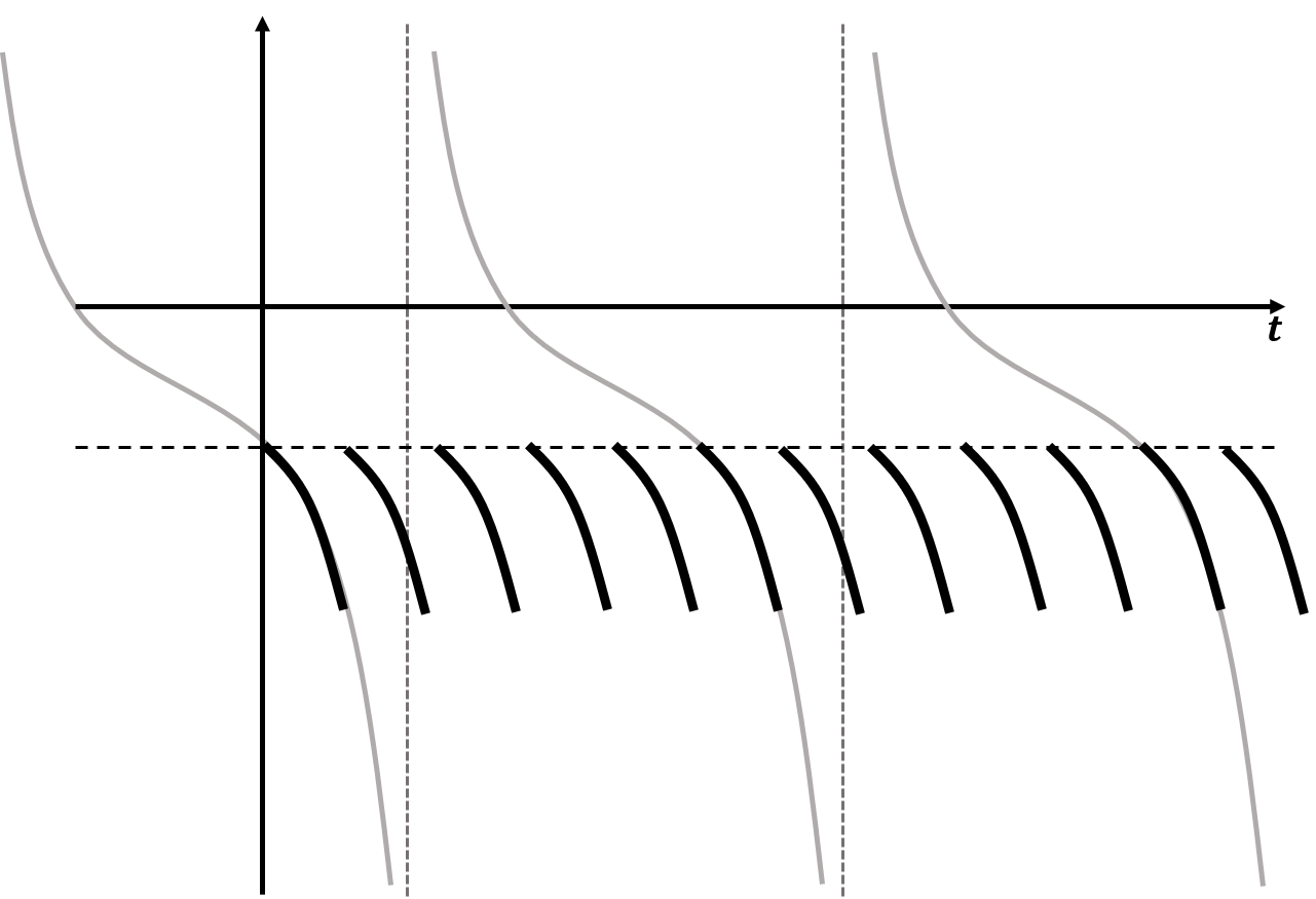
Figure 1: Graph of the function $\underline{\varphi}$

Our goal is to show that $u_{r}\geq\underline{\varphi}$. Toward this goal, in view of the comparison principle, it is enough to verify that $\mathcal{P}\underline{\varphi}\leq 0$. Since $\underline{\varphi}$ is a monotonically decreasing function with respect to $t\in\left(\frac{(6n-6+j)\pi}{6\widetilde{c_{4}}\sqrt{\widetilde{C}}},\frac{(6n-5+j)\pi}{6\widetilde{c_{4}}\sqrt{\widetilde{C}}}\right]$ for all $n\in\mathbb{N}$ and all $j\in\{0,1,2,3,4,5\}$, it follows that

$$\underline{\varphi}(r,t)\leq\underline{\varphi}(r,0)<-E$$

for all $r\in(0,R)$ and all $t\in(0,T_{\rm max})$, and hence

$$\underline{\varphi}<0.$$

Noting that

$$\underline{\varphi}_{r}=\underline{\varphi}_{rr}=0\quad\mbox{and}\quad-\underline{\varphi}=|\underline{\varphi}|$$

because $\underline{\varphi}$ is independent of $r$ and $\underline{\varphi}<0$, we obtain from (2.4) that

$$(\mathcal{P}\underline{\varphi})(r,t) ={\underline{\varphi}}_{t}-a_{3}(r,t){\underline{\varphi}}^{2}+A_{3}(r,t)|\underline{\varphi}|-A_{4}(r,t)$$

$$={\underline{\varphi}}_{t}-\left(p(p-1)\frac{u^{p-2}u^{5}_{r}}{{\sqrt{u^{2}+u^{2}_{r}}}^{5}}-q(q-1)\chi\frac{u^{q-2}v_{r}}{\sqrt{1+v^{2}_{r}}}\right){\underline{\varphi}}^{2}$$

$$\quad\,+p(p-4)\frac{u^{p}u^{4}_{r}}{{\sqrt{u^{2}+u^{2}_{r}}}^{5}}|\underline{\varphi}|-\frac{n-1}{r^{2}}\cdot\frac{u^{p}}{\sqrt{u^{2}+u^{2}_{r}}}|\underline{\varphi}|$$

$$\quad\,+(p-1)(p-2)\frac{u^{p+2}u_{r}}{{\sqrt{u^{2}+u^{2}_{r}}}^{5}}|\underline{\varphi}|+(p-1)(p+1)\frac{u^{p}u^{3}_{r}}{{\sqrt{u^{2}+u^{2}_{r}}}^{5}}|\underline{\varphi}|$$

$$\quad\,-q\chi\mu\frac{u^{q-1}}{{\sqrt{1+v^{2}_{r}}}^{3}}|\underline{\varphi}|+(q+1)\chi\frac{u^{q}}{{\sqrt{1+v^{2}_{r}}}^{3}}|\underline{\varphi}|-q\chi\frac{u^{q-1}v_{rr}}{{\sqrt{1+v^{2}_{r}}}^{3}}|\underline{\varphi}|$$

$$\quad\,+q\chi\frac{u^{q-1}v^{2}_{r}v_{rr}}{{\sqrt{1+v^{2}_{r}}}^{3}}|\underline{\varphi}|-q\chi\frac{n-1}{r}\cdot\frac{u^{q-1}v^{3}_{r}}{{\sqrt{1+v^{2}_{r}}}^{3}}|\underline{\varphi}|$$

$$\quad\,-p\frac{n-1}{r}\cdot\frac{u^{p-1}u^{4}_{r}}{{\sqrt{u^{2}+u^{2}_{r}}}^{3}}-(p-1)\frac{n-1}{r}\cdot\frac{u^{p+1}u^{2}_{r}}{{\sqrt{u^{2}+u^{2}_{r}}}^{3}}-3\chi\mu\frac{u^{q}v_{r}v_{rr}}{{\sqrt{1+v^{2}_{r}}}^{5}}$$

$$\quad\,+3\chi\frac{u^{q+1}v_{r}v_{rr}}{{\sqrt{1+v^{2}_{r}}}^{5}}-\chi\frac{n-1}{r^{2}}\cdot\frac{u^{q}v^{3}_{r}}{{\sqrt{1+v^{2}_{r}}}^{3}}+3\chi\frac{n-1}{r}\cdot\frac{u^{q}v^{2}_{r}v_{rr}}{{\sqrt{1+v^{2}_{r}}}^{5}}$$

for all $r\in(0,R)$ and all $t\in(0,T_{\rm max})$. Then, since $\underline{\varphi}$ satisfies

$${\underline{\varphi}}_{t}=-\widetilde{c_{4}}{\underline{\varphi}}^{2}+\widetilde{c_{5}}\underline{\varphi}-\widetilde{c_{6}}$$

and the fourth, seventh, twelfth, thirteenth terms on the right-hand side are nonpositive:

$$-\frac{n-1}{r^{2}}\cdot\frac{u^{p}}{\sqrt{u^{2}+u^{2}_{r}}}|\underline{\varphi}|\leq 0,\qquad-q\chi\mu\frac{u^{q-1}}{{\sqrt{1+v^{2}_{r}}}^{3}}|\underline{\varphi}|\leq 0,$$

$$-p\frac{n-1}{r}\cdot\frac{u^{p-1}u^{4}_{r}}{{\sqrt{u^{2}+u^{2}_{r}}}^{3}}\leq 0,\qquad-(p-1)\frac{n-1}{r}\cdot\frac{u^{p+1}u^{2}_{r}}{{\sqrt{u^{2}+u^{2}_{r}}}^{3}}\leq 0,$$

we can obtain from (4.1), (4.2) and the inequality e.g. $\frac{u^{5}_{r}}{\sqrt{u^{2}+u^{2}_{r}}^{5}}\leq 1$ that

$$(\mathcal{P}\underline{\varphi})(r,t) \leq{\underline{\varphi}}_{t}+\left(p(p-1)c^{p-2}_{1}+q(q-1)\chi c^{q-2}_{1}\right){\underline{\varphi}}^{2}$$

$$\quad\,+\left(3p(p+1)c^{p-2}_{1}+q(c_{1}+2c_{3}+\mu)\chi c^{q-1}_{1}\right)|\underline{\varphi}|$$

$$\quad\,+3\left(\mu c_{3}+c_{1}c_{3}+\frac{(n-1)c^{2}_{2}}{3}+(n-1)c_{2}c_{3}\right)\chi c^{q}_{1}c_{2}R$$

$$=-\widetilde{c_{4}}{\underline{\varphi}}^{2}+\widetilde{c_{5}}\underline{\varphi}-\widetilde{c_{6}}+c_{4}{\underline{\varphi}}^{2}+c_{5}|\underline{\varphi}|+c_{6}$$

$$=(c_{4}-\widetilde{c_{4}}){\underline{\varphi}}^{2}+(c_{5}-\widetilde{c_{5}})|\underline{\varphi}|+(c_{6}-\widetilde{c_{6}})$$

for all $r\in(0,R)$ and all $t\in(T_{\rm max}-\varepsilon,T_{\rm max})$. Then the relations that $\widetilde{c_{4}}>c_{4}$, $\widetilde{c_{5}}>c_{5}$ and $\widetilde{c_{6}}>c_{6}$ ensure that

$$(\mathcal{P}\underline{\varphi})(r,t)\leq 0$$

for all $r\in(0,R)$ and all $t\in(T_{\rm max}-\varepsilon,T_{\rm max})$. Since

$$(\mathcal{P}u_{r})(r,t)=0$$

for all $(r,t)\in(0,R)\times(T_{\rm max}-\varepsilon,T_{\rm max})$, and moreover

$$\underline{\varphi}(r,T_{\rm max}-\varepsilon) <\underline{\varphi}(r,0)$$

$$=\frac{1}{2\widetilde{c_{4}}}\left(\frac{2}{3}+\alpha_{1}\right)\tan{\frac{-\pi}{3\cdot\left(\frac{2}{3}+\alpha_{1}\right)}}+\frac{\widetilde{c_{5}}}{2\widetilde{c_{4}}}$$

$$<-E$$

$$\leq u_{r}(r,T_{\rm max}-\varepsilon)$$

for all $r\in[0,R]$ and

$$\underline{\varphi}(0,t)\leq u_{r}(0,t)=0,$$

$$\underline{\varphi}(R,t)\leq u_{r}(R,t)=0$$

for all $t\in(T_{\rm max}-\varepsilon,T_{\rm max})$, the comparison principle derives that $u_{r}(r,t)\geq\underline{\varphi}(r,t)$ for all $r\in(0,R)$ and all $t\in(T_{\rm max}-\varepsilon,T_{\rm max})$, and hence

$$u_{r}(r,t) \geq\underline{\varphi}(r,T_{\rm max})$$

$$=-|\underline{\varphi}(r,T_{\rm max})|$$

for all $t\in(T_{\rm max}-\varepsilon,T_{\rm max})$. Therefore by putting

$$C:=\max\left\{|\underline{\varphi}(r,T_{\rm max})|,\,\max_{(r,t)\in(0,R)\times(0,T_{\rm max}-\varepsilon)}{|u_{r}(r,t)|}\right\}$$

we have this lemma. ∎

5 A bound for $|u_{r}|$. Proof of Theorem 1.1

5.1 A bound for $|u_{r}|$ in terms of $z_{+}$

Thanks to Lemma 4.1, in order to rule out the possibility of gradient blow-up, it is enough to see that $u_{r}\leq C$ with some $C>0$. Here, in view of arguments as in [2, Section 5], we will establish a bound for $u_{r}$ in terms of $z_{+}$. First we rewrite (2.2) in Lemma 2.2 by multiplying $\frac{1}{u}$ on the both sides and find a key quantity such that

(5.1) $$z:=\frac{u_{t}}{u} =\frac{u^{p+1}u_{rr}}{{\sqrt{u^{2}+u^{2}_{r}}}^{3}}+p\frac{u^{p-2}u^{4}_{r}}{{\sqrt{u^{2}+u^{2}_{r}}}^{3}}+\frac{n-1}{r}\cdot\frac{u^{p-1}u_{r}}{\sqrt{u^{2}+u^{2}_{r}}}+(p-1)\frac{u^{p}u^{2}_{r}}{{\sqrt{u^{2}+u^{2}_{r}}}^{3}}$$

$$\quad\,-q\chi\frac{u^{q-2}u_{r}v_{r}}{\sqrt{1+v^{2}_{r}}}-\chi\frac{u^{q-1}(\mu-u)}{{\sqrt{1+v^{2}_{r}}}^{3}}-\chi\frac{n-1}{r}\cdot\frac{u^{q-1}v^{3}_{r}}{{\sqrt{1+v^{2}_{r}}}^{3}}.$$

This plays an important role when we establish an estimate for $u_{r}$ which derives the desired extensibility criterion.

Lemma 5.1.

Assume that $T_{\rm max}<\infty$,  but that $\sup_{(r,t)\in(0,R)\times(0,T_{\rm max})}u(r,t)<\infty.$  Then there exist $R_{0}\in(0,R)$ and a constant $C>0$ such that

$${\|u_{r}(\cdot,t)\|}_{L^{\infty}(0,R_{0})}\leq C\left(1+{\|z_{+}(\cdot,t)\|}_{L^{\infty}(0,R_{0})}\right)$$

for all $t\in(0,T_{\rm max})$.

Proof.

The proof is based on an argument in the proof of [2, Lemma 5.1]. We rewrite (5.1) to have

(5.2) $$p\frac{u^{4}_{r}}{u^{3}} =\frac{{\sqrt{u^{2}+u^{2}_{r}}}^{3}}{u^{p+1}}z-u_{rr}-\frac{n-1}{r}u_{r}\cdot\frac{{\sqrt{u^{2}+u^{2}_{r}}}^{2}}{u^{2}}-(p-1)\frac{u^{2}_{r}}{u}$$

$$\quad\,+q\chi\frac{{\sqrt{u^{2}+u^{2}_{r}}}^{3}\cdot u_{r}v_{r}}{u^{p-q+3}\sqrt{1+v^{2}_{r}}}+\chi\frac{{\sqrt{u^{2}+u^{2}_{r}}}^{3}(\mu-u)}{u^{p-q+2}{\sqrt{1+v^{2}_{r}}}^{3}}$$

$$\quad\,+\chi\frac{n-1}{r}\cdot\frac{{\sqrt{u^{2}+u^{2}_{r}}}^{3}v^{3}_{r}}{u^{p-q+2}{\sqrt{1+v^{2}_{r}}}^{3}},$$

and we have from the identity $u_{rr}+\frac{n-1}{r}u_{r}=\frac{1}{r^{n-1}}(r^{n-1}u_{r})_{r}$ that

(5.3) $$-u_{rr}-\frac{n-1}{r}u_{r}\cdot\frac{{\sqrt{u^{2}+u^{2}_{r}}}^{2}}{u^{2}} =-\left(u_{rr}+\frac{n-1}{r}u_{r}\right)-\frac{n-1}{r}\cdot\frac{u^{3}_{r}}{u^{2}}$$

$$=-\frac{1}{r^{n-1}}(r^{n-1}u_{r})_{r}-\frac{n-1}{r}\cdot\frac{u^{3}_{r}}{u^{2}}$$

for all $r\in(0,R)$ and all $t\in(0,T_{\rm max})$. Thanks to the assumption of the boundedness of $u$, we can take constants $c_{1}\geq\mu$ and $c_{2}>0$ such that

$$u\leq c_{1}\quad\mbox{and}\quad\sqrt{u^{2}+u^{2}_{r}}^{3}\leq c_{2}(1+{|u_{r}|}^{3})$$

for all $r\in(0,R)$ and all $t\in(0,T_{\rm max})$. On the other hand, recalling Lemma 3.1, we can find a constant $c_{3}>0$ fulfilling

(5.4) $$u\geq c_{3}\qquad$$

for all $r\in(0,R)$ and all $t\in(0,T_{\rm max})$. Because of the estimate $c_{3}\leq u\leq c_{1}$ for all $r\in(0,R)$ and all $t\in(0,T_{\rm max})$, we can obtain constants $C(p,q)>0$ and $\widetilde{C}(p,q)>0$ such that

$$u^{p-q+3}\geq C(p,q)\quad\mbox{and}\quad u^{p-q+2}\geq\widetilde{C}(p,q)$$

for all $r\in(0,R)$ and all $t\in(0,T_{\rm max})$. In order to show that the conclusion of this lemma holds, we pick any $R_{0}\in(0,R)$ satisfying

$$R_{0}\leq\frac{nC(p,q)}{4c^{3}_{1}c_{2}q\chi\mu}.$$

Here, let $m$ be an arbitrary even integer and introduce

$$I(t):=p\int_{0}^{R_{0}}r^{n-1}\frac{u^{m+4}_{r}}{u^{3}}\,dr.$$

By using the lower estimate (5.4) for $u$ we first obtain

(5.5) $$I(t)\geq\frac{p}{c^{3}_{3}}\int_{0}^{R_{0}}r^{n-1}u^{m+4}_{r}\,dr\geq\frac{1}{c^{3}_{3}}\int_{0}^{R_{0}}r^{n-1}u^{m+4}_{r}\,dr$$

for all $t\in(0,T_{\rm max})$. On the other hand, we multiply the quantity $r^{n-1}u^{m}_{r}$ on the both sides of (5.2), integrate over $(0,R_{0})$ and use (5.3) to establish that

(5.6) $$I(t) =p\int_{0}^{R_{0}}r^{n-1}\frac{u^{m+4}_{r}}{u^{3}}\,dr$$

$$=\int_{0}^{R_{0}}r^{n-1}\frac{{\sqrt{u^{2}+u^{2}_{r}}}^{3}}{u^{p+1}}u^{m}_{r}z\,dr-\int_{0}^{R_{0}}(r^{n-1}u_{r})_{r}\cdot u^{m}_{r}\,dr$$

$$\quad\,-\int_{0}^{R_{0}}r^{n-2}\cdot\frac{u^{m+3}_{r}}{u^{2}}\,dr-(p-1)\int_{0}^{R_{0}}r^{n-1}\cdot\frac{u^{m+2}_{r}}{u}\,dr$$

$$\quad\,+\chi\int_{0}^{R_{0}}r^{n-1}\frac{(\mu-u){\sqrt{u^{2}+u^{2}_{r}}}^{3}u^{m}_{r}}{u^{p-q+2}{\sqrt{1+v^{2}_{r}}}^{3}}\,dr$$

$$\quad\,+q\chi\int_{0}^{R_{0}}r^{n-1}\frac{{\sqrt{u^{2}+u^{2}_{r}}}^{3}\cdot u^{m+1}_{r}v_{r}}{u^{p-q+3}\sqrt{1+v^{2}_{r}}}\,dr$$

$$\quad\,+(n-1)\chi\int_{0}^{R_{0}}r^{n-2}\frac{{\sqrt{u^{2}+u^{2}_{r}}}^{3}u^{m}_{r}v^{3}_{r}}{u^{p-q+2}{\sqrt{1+v^{2}_{r}}}^{3}}\,dr.$$

Since the fact that $m+2$ is even means that the fourth term of the right-hand side on (5.6) is nonpositive, combining (5.5) with (5.6) implies that

(5.7) $$\frac{1}{c^{3}_{3}}\int_{0}^{R_{0}}r^{n-1}u^{m+4}_{r}\,dr \leq\int_{0}^{R_{0}}r^{n-1}\frac{{\sqrt{u^{2}+u^{2}_{r}}}^{3}}{u^{p+1}}u^{m}_{r}z\,dr-\int_{0}^{R_{0}}(r^{n-1}u_{r})_{r}\cdot u^{m}_{r}\,dr$$

$$\quad\,-\int_{0}^{R_{0}}r^{n-2}\cdot\frac{u^{m+3}_{r}}{u^{2}}\,dr$$

$$\quad\,+\chi\int_{0}^{R_{0}}r^{n-1}\frac{(\mu-u){\sqrt{u^{2}+u^{2}_{r}}}^{3}u^{m}_{r}}{u^{p-q+2}{\sqrt{1+v^{2}_{r}}}^{3}}\,dr$$

$$\quad\,+q\chi\int_{0}^{R_{0}}r^{n-1}\frac{{\sqrt{u^{2}+u^{2}_{r}}}^{3}\cdot u^{m+1}_{r}v_{r}}{u^{p-q+3}\sqrt{1+v^{2}_{r}}}\,dr$$

$$\quad\,+(n-1)\chi\int_{0}^{R_{0}}r^{n-2}\frac{{\sqrt{u^{2}+u^{2}_{r}}}^{3}u^{m}_{r}v^{3}_{r}}{u^{p-q+2}{\sqrt{1+v^{2}_{r}}}^{3}}\,dr$$

$$=:J_{1}(t)+J_{2}(t)+J_{3}(t)+J_{4}(t)+J_{5}(t)+J_{6}(t)$$

for all $t\in(0,T_{\rm max})$. Then we shall show estimates for $J_{i}$ ($i\in\{1,2,3,4,5,6\}$) from an argument similar to that in the proof of [2, Lemma 5.1]. Employing the Young inequality and the H$\ddot{\mbox{o}}$lder inequality, we have that for all $t\in(0,T_{\rm max})$,

(5.8) $$J_{1}(t)\leq c_{4}\left[1+\left(\int_{0}^{R_{0}}r^{n-1}u^{m+4}_{r}\,dr\right)^{\frac{m+3}{m+4}}\right]\left(\int_{0}^{R_{0}}r^{n-1}z^{m+4}_{+}\,dr\right)^{\frac{1}{m+4}}$$

with $c_{4}:=\max\{\frac{c_{2}}{c_{3}^{p+1}}\cdot\frac{R^{n}_{1}}{n},\frac{2c_{2}}{c_{3}^{p+1}}\}\,$ and $R_{1}:=\max\{1,R\}$, and that

(5.9) $$J_{2}(t)\leq R^{n-1}\cdot L^{m+1},\quad J_{3}(t)\leq\frac{R^{n-1}}{C^{2}_{3}}\cdot L^{m+3}$$

(5.10) $$J_{4}(t)\leq c_{5}\left[1+\left(\int_{0}^{R_{0}}r^{n-1}u^{m+4}_{r}\,dr\right)^{\frac{m+3}{m+4}}\right]$$

with $c_{5}:=\max\{\frac{c_{2}\chi\mu}{n\widetilde{C}(p,q)}\cdot\frac{R^{n}_{1}}{n},\,\frac{2c_{2}\chi\mu}{n\widetilde{C}(p,q)}\cdot\frac{R^{n}_{1}}{n}\}$, as well as that

(5.11) $$J_{5}(t)\leq\left(c_{6}+\frac{1}{2c^{3}_{3}}\int_{0}^{R_{0}}r^{n-1}u^{m+4}_{r}\,dr\right)+\left(c_{7}+\frac{c_{8}}{m+4}\int_{0}^{R_{0}}r^{n-1}u^{m+4}_{r}\,dr\right)$$

with $c_{6}:=\frac{q\chi\mu c_{2}R_{0}^{n+1}}{n(n+1)C(p,q)}$, $c_{7}:=\frac{2q\chi\mu c_{1}c_{2}R_{0}^{n+1}}{n(n+1)C(p,q)}$ and $c_{8}:=\frac{3q\chi\mu c_{1}c_{2}R}{nC(p,q)}$ and that

(5.12) $$J_{6}(t)\leq c_{9}\left[1+\left(\int_{0}^{R_{0}}r^{n-1}u^{m+4}_{r}\,dr\right)^{\frac{m+3}{m+4}}\right]$$

with $c_{9}:=\max\{\frac{2c_{2}(n-1)\chi\mu R^{n}_{0}}{3\sqrt{3}n^{2}\widetilde{C}(p,q)},\frac{4c_{2}(n-1)\chi\mu}{3\sqrt{3}\widetilde{C}(p,q)}\cdot\frac{R^{n}_{1}}{n}\}$. In summary, (5.8)–(5.12) combined with (5.7) show that

$$\frac{1}{c^{3}_{3}}\int_{0}^{R_{0}}r^{n-1}u^{m+4}_{r}\,dr \leq c_{4}\left[1+\left(\int_{0}^{R_{0}}r^{n-1}u^{m+4}_{r}\,dr\right)^{\frac{m+3}{m+4}}\right]\left(\int_{0}^{R_{0}}r^{n-1}z^{m+4}_{+}\,dr\right)^{\frac{1}{m+4}}$$

$$\quad\,+R^{n-1}\cdot L^{m+1}+\frac{R^{n-1}}{C^{2}_{3}}\cdot L^{m+3}+c_{5}\left[1+\left(\int_{0}^{R_{0}}r^{n-1}u^{m+4}_{r}\,dr\right)^{\frac{m+3}{m+4}}\right]$$

$$\quad\,+c_{6}+\frac{1}{2c^{3}_{3}}\int_{0}^{R_{0}}r^{n-1}u^{m+4}_{r}\,dr+c_{7}+\frac{c_{8}}{m+4}\int_{0}^{R_{0}}r^{n-1}u^{m+4}_{r}\,dr$$

$$\quad\,+c_{9}\left[1+\left(\int_{0}^{R_{0}}r^{n-1}u^{m+4}_{r}\,dr\right)^{\frac{m+3}{m+4}}\right]$$

for all $t\in(0,T_{\rm max})$. Here, we put $m_{0}>0$ satisfying $\frac{c_{8}}{m_{0}+4}\leq\frac{1}{4c^{3}_{3}}$. Then the above inequality implies that for all $m\geq m_{0}$,

(5.13) $$\frac{1}{4c^{3}_{3}}\int_{0}^{R_{0}}r^{n-1}u^{m+4}_{r}\,dr \leq c_{4}\left[1+\left(\int_{0}^{R_{0}}r^{n-1}u^{m+4}_{r}\,dr\right)^{\frac{m+3}{m+4}}\right]\left(\int_{0}^{R_{0}}r^{n-1}z^{m+4}_{+}\,dr\right)^{\frac{1}{m+4}}$$

$$\quad\,+c_{10}\left(\int_{0}^{R_{0}}r^{n-1}u^{m+4}_{r}\,dr\right)^{\frac{m+3}{m+4}}+c_{11}L^{m+4}$$

holds with some $c_{10},c_{11}>0$. In order to establish the conclusion of this lemma, we fix $t\geq 0$ and first deal with the case that there exists a sequence of even numbers $m=m_{j}\geq m_{0}$, $j\in\mathbb{N}$ satisfying $m_{j}\to\infty$ as $j\to\infty$ and $\left(\int_{0}^{R_{0}}r^{n-1}u^{m+4}_{r}\,dr\right)^{\frac{m+3}{m+4}}\leq L^{m+4}$ for all $m\in(m_{j})_{j\in\mathbb{N}}$. Then taking the limit $j\to\infty$ implies that

$$\|u_{r}(\cdot,t)\|_{L^{\infty}(0,R_{0})}=\lim_{j\to\infty}\left(\int_{0}^{R_{0}}r^{n-1}u_{r}^{m_{j}+4}\,dr\right)^{\frac{1}{m_{j}+4}}=\lim_{j\to\infty}L^{\frac{m_{j}+3}{m_{j}+4}}=L.$$

We next consider the case that there is no such a sequence. Then we can pick $\widetilde{m_{0}}\geq m_{0}$ such that

$$\left(\int_{0}^{R_{0}}r^{n-1}u^{m+4}_{r}\,dr\right)^{\frac{m+3}{m+4}}>L^{m+4}$$

for all even $m\geq\widetilde{m_{0}}$. Plugging this inequality into (5.13) and noting the fact that $L\geq 1$, we obtain that

$$\frac{1}{4c^{3}_{3}}\left(\int_{0}^{R_{0}}r^{n-1}u^{m+4}_{r}\,dr\right)^{\frac{1}{m+4}}\leq 2c_{4}\left(\int_{0}^{R_{0}}r^{n-1}z^{m+4}_{+}\,dr\right)^{\frac{1}{m+4}}+c_{10}+c_{11}.$$

Taking the limit $m\to\infty$, we can see that

$$\frac{1}{4c^{3}_{3}}\|u_{r}(\cdot,t)\|_{L^{\infty}(0,R_{0})}\leq 2c_{4}\|z_{+}(\cdot,t)\|_{L^{\infty}(0,R_{0})}+c_{10}+c_{11}$$

holds for all $t\in(0,T_{\rm max})$. ∎

Lemma 5.1 gives us the estimate for $\|u_{r}(\cdot,t)\|_{L^{\infty}(0,R_{0})}$ with some $R_{0}$. This means that we have boundedness of $u_{r}$ only on $(0,R_{0})$. Next, we obtain an estimate for $\|u_{r}(\cdot,t)\|_{L^{\infty}(R_{0},R)}$.

Lemma 5.2.

Assume that $T_{\rm max}<\infty$, but that $\sup_{(r,t)\in(0,R)\times(0,T_{\rm max})}u(r,t)<\infty$. Then with $R_{0}\in(0,R)$ taken from Lemma 5.1, for all $t_{0}>0$ there exists a constant $C>0$ such that

$${\|u_{r}(\cdot,t)\|}_{L^{\infty}(R_{0},R)}\leq C\left(1+{\|z_{+}\|}_{L^{\infty}((0,R_{0})\times(t_{0},t))}\right)$$

for all $t\in(t_{0},T_{\rm max})$.

Proof.

Thanks to Lemma 5.1, we can find a constant $c_{1}>0$ such that

(5.14) $$u_{r}(R_{0},t)\leq c_{1}\left(1+{\|z_{+}(\cdot,t)\|}_{L^{\infty}(0,R_{0})}\right)$$

for all $t\in(0,T_{\rm max})$. Now we pick $t_{0}\in(0,T_{\rm max})$. In particular, (5.14) implies that, given any $t_{1}\in(t_{0},T_{\rm max})$, we have

(5.15) $$u_{r}(R_{0},t)\leq D_{1}(t_{0},t_{1}):=c_{1}\left(1+{\|z_{+}\|}_{L^{\infty}((0,R_{0})\times(t_{0},t_{1}))}\right)$$

for all $t\in(t_{0},t_{1})$. Next, we use the assumption and recall Lemma 3.1 to pick $c_{2}>0$ and $c_{3}>0$ such that

$$c_{2}\leq u(r,t)\leq c_{3}\qquad$$

for all $r\in(0,R)$ and all $t\in(0,T_{\rm max})$. Moreover, Lemma 2.5 yields existence of constants $c_{4}>0$ and $c_{5}>0$ such that

$$|v_{r}(r,t)|\leq c_{4}r\quad\mbox{and}\quad|v_{rr}(r,t)|\leq c_{5}$$

for all $r\in(0,R)$ and all $t\in(0,T_{\rm max})$. Therefore, the functions $a_{3}(r,t)$, $\widetilde{A_{3}}(r,t)$ and $\widetilde{A_{4}}(r,t)$ in (2.6) can be estimated according to

(5.16) $$a_{3}(r,t)\leq c_{6} :=p(p-1)c^{p-2}_{3}+q(q-1)\chi c^{q-2}_{3},$$

(5.17) $$\widetilde{A_{3}}(r,t)\leq c_{7} :=\frac{(2p-1)(n-1)}{R_{0}}\cdot c^{p-1}_{3}+p(3p+1)c^{p-1}_{3}$$

$$\quad\ +(q+2)\chi c^{q}_{3}+q\chi c^{q-1}_{3}c^{2}_{4}R^{2}c_{5}+q\chi(n-1)c^{q-1}_{3}c^{3}_{4}R^{2}$$

and

(5.18) $$\widetilde{A_{4}}(r,t)\leq c_{8} :=\frac{n-1}{R_{0}}\cdot c^{p-1}_{3}+3\chi\mu c^{q}_{3}c_{4}Rc_{5}+3\chi c^{q-1}_{3}c_{4}Rc_{5}$$

$$\quad\ +\chi(n-1)c^{q}_{3}c^{3}_{4}R+3\chi(n-1)c^{q}_{3}c^{2}_{4}R{c_{5}}$$

for all $r\in(0,R)$ and all $t\in(0,T_{\rm max})$. We now take $\widetilde{c_{6}}>0$ and $\widetilde{c_{7}}>0$ fulfilling $\widetilde{c_{6}}>c_{6}$, $\widetilde{c_{7}}>c_{7}$ and

(5.19) $$4\widetilde{c_{6}}c_{8}-{\widetilde{c_{7}}}^{2}<0.$$

Then there exist $n\in\mathbb{N}$ and $j\in\{0,1,2,3,4,5\}$ such that

$$2\cdot\frac{(6n-5+j)\pi}{6\cdot\frac{2}{3}}<t_{1}<2\cdot\frac{(6n-6+j)\pi}{6\cdot\frac{2}{3}}.$$

Therefore we can find $\varepsilon>0$ such that

$$2\cdot\frac{(6n-5+j)\pi}{6\cdot\frac{2}{3}}<t_{1}-\varepsilon<t_{1}<2\cdot\frac{(6n-6+j)\pi}{6\cdot\frac{2}{3}},$$

and then there exists $\alpha_{0}>0$ such that

(5.20) $$2\cdot\frac{(6n-5+j)\pi}{6\cdot(\frac{2}{3}+\alpha)}<t_{1}-\varepsilon<t_{1}<2\cdot\frac{(6n-6+j)\pi}{6\cdot(\frac{2}{3}+\alpha)}$$

for all $\alpha\in(0,{\alpha}_{0})$. Since $x\tan{\frac{\pi}{3x}}\to\infty$ as $x\searrow\frac{2}{3}$, we can find $\alpha_{1}\in(0,\alpha_{0})$ such that

$$\max\left\{D_{1}(t_{0},t_{1}),\ \sup_{r\in(0,R)}{u_{r}(r,T_{\rm max}-\varepsilon)}\right\}\leq\frac{1}{2\widetilde{c_{6}}}\left(\frac{2}{3}+\alpha_{1}\right)\tan{\frac{\pi}{3\cdot\left(\frac{2}{3}+\alpha_{1}\right)}}-\frac{\widetilde{c_{7}}}{2\widetilde{c_{6}}}.$$

Aided by (5.19) and the fact that $4\widetilde{c_{6}}x-{\widetilde{c_{7}}}^{2}\to\infty$ as $x\to\infty$, we obtain from the intermediate value theorem that there is a constant $\widetilde{c_{8}}>c_{8}$ such that

(5.21) $$\sqrt{4\widetilde{c_{6}}\widetilde{c_{8}}-{\widetilde{c_{7}}}^{2}}=\frac{2}{3}+\alpha_{1}.$$

Combination of (5.20) and (5.21) with $\alpha=\alpha_{1}$ implies that

$$\frac{(6n-6+j)\pi}{6\cdot\sqrt{\frac{4\widetilde{c_{6}}\widetilde{c_{8}}-{\widetilde{c_{7}}}^{2}}{4}}}<t_{1}-\varepsilon<t_{1}<\frac{(6n-5+j)\pi}{6\cdot\sqrt{\frac{4\widetilde{c_{6}}\widetilde{c_{8}}-{\widetilde{c_{7}}}^{2}}{4}}}.$$

We define a comparison function $\overline{\varphi}$ by letting

$$\overline{\varphi}(r,t):=\begin{cases}D-\frac{\widetilde{c_{7}}}{2\widetilde{c_{6}}},&t=0,\\[14.22636pt] \sqrt{\widetilde{C}}\tan\left[\tan^{-1}\frac{D}{\sqrt{\widetilde{C}}}+\widetilde{c_{6}}\sqrt{\widetilde{C}}\left(t-\frac{j\pi}{6\widetilde{c_{6}}\sqrt{\widetilde{C}}}\right)\right]-\frac{\widetilde{c_{7}}}{2\widetilde{c_{6}}},&t\in\left(\frac{(6n-6+j)\pi}{6\widetilde{c_{6}}\sqrt{\widetilde{C}}},\frac{(6n-5+j)\pi}{6\widetilde{c_{6}}\sqrt{\widetilde{C}}}\right]\end{cases}$$

for $r\in[R_{0},R]$, $t\in[t_{0},t_{1}]$, $n\in\mathbb{N}$ and $j\in\{0,1,2,3,4,5\}$, where

$$\widetilde{C}:=\frac{4\widetilde{c_{6}}\widetilde{c_{8}}-{\widetilde{c_{7}}}^{2}}{4{\widetilde{c_{6}}}^{2}}\quad\mbox{and}\quad D:=\frac{1}{2\widetilde{c_{6}}}\left(\frac{2}{3}+\alpha_{1}\right)\tan{\frac{\pi}{3\cdot\left(\frac{2}{3}+\alpha_{1}\right)}}.$$

Here we can verify that

$$\overline{\varphi}(r,t)\geq\overline{\varphi}(r,0)>0$$

for all $r\in(R_{0},R)$ and all $t\in(0,T_{\rm max})$ since $\overline{\varphi}$ is a monotonically increasing function with respect to $t\in\left(\frac{(6n-6+j)\pi}{6\widetilde{c_{6}}\sqrt{\widetilde{C}}},\frac{(6n-5+j)\pi}{6\widetilde{c_{6}}\sqrt{\widetilde{C}}}\right]$ for all $n\in\mathbb{N}$ and all $j\in\{0,1,2,3,4,5\}$. Moreover, from the facts that $\overline{\varphi}_{r}=\overline{\varphi}_{rr}\equiv 0$ and that ${\overline{\varphi}}_{t}=\widetilde{c_{6}}{\overline{\varphi}}^{2}+\widetilde{c_{7}}\overline{\varphi}+\widetilde{c_{8}}$, we use (5.16), (5.17) and (5.18) to see that with $\mathcal{Q}$ as in (2.5) we have

$$(\mathcal{Q}\overline{\varphi})(r,t) ={\overline{\varphi}}_{t}-a_{3}(r,t){\overline{\varphi}}^{2}-\widetilde{A_{3}}(r,t)\overline{\varphi}-\widetilde{A_{4}}(r,t)$$

$$\geq{\overline{\varphi}}_{t}-|a_{3}(r,t)|{\overline{\varphi}}^{2}-|\widetilde{A_{3}}(r,t)|\overline{\varphi}-|\widetilde{A_{4}}(r,t)|$$

$$\geq{\overline{\varphi}}_{t}-c_{6}{\overline{\varphi}}^{2}-c_{7}\overline{\varphi}-c_{8}$$

$$=(\widetilde{c_{6}}-c_{6}){\overline{\varphi}}^{2}+(\widetilde{c_{7}}-c_{7})\overline{\varphi}+(\widetilde{c_{8}}-c_{8})$$

for all $r\in(R_{0},R)$ and all $t\in[t_{1}-\varepsilon,t_{1}]$. Then the relations that $\widetilde{c_{6}}>c_{6},\,\widetilde{c_{7}}>c_{7}$ and $\widetilde{c_{8}}>c_{8}$ ensure that

$$(\mathcal{Q}\overline{\varphi})(r,t)>0$$

for all $r\in(R_{0},R)$ and all $t\in(t_{1}-\varepsilon,t_{1})$. Since

$$(\mathcal{Q}u_{r})(r,t)=0$$

for all $(r,t)\in(R_{0},R)\times(t_{0},t_{1})$, and since

$$u_{r}(r,t_{1}-\varepsilon) <\sup_{r\in(0,R)}u_{r}(r,t_{1}-\varepsilon)$$

$$\leq\frac{1}{2\widetilde{c_{6}}}\left(\frac{2}{3}+\alpha_{1}\right)\tan{\frac{\pi}{3\cdot\left(\frac{2}{3}+\alpha_{1}\right)}}-\frac{\widetilde{c_{7}}}{2\widetilde{c_{6}}}=\overline{\varphi}(r,0)\leq\overline{\varphi}(r,t_{1}-\varepsilon)$$

for all $r\in[R_{0},R]$ and

$$0=u_{r}(R,t)\leq\overline{\varphi}(R,t)$$

for all $t\in[t_{1}-\varepsilon,t_{1}]$ and moreover

$$u_{r}(R_{0},t)\leq D_{1}(t_{0},t_{1}) \leq\frac{1}{2\widetilde{c_{6}}}\left(\frac{2}{3}+\alpha_{1}\right)\tan{\frac{\pi}{3\cdot\left(\frac{2}{3}+\alpha_{1}\right)}}-\frac{\widetilde{c_{7}}}{2\widetilde{c_{6}}}=\overline{\varphi}(r,0)\leq\overline{\varphi}(r,t)$$

for all $r\in[R_{0},R]$ and all $t\in[t_{1}-\varepsilon,t_{1}]$, in particular, $u_{r}(R_{0},t)\leq\overline{\varphi}(R_{0},t)$ for all $t\in[t_{1}-\varepsilon,t_{1}]$, the comparison principle derives that $u_{r}(r,t)\leq\overline{\varphi}(r,t)$ for all $r\in[R_{0},R]$ and all $t\in[t_{1}-\varepsilon,t_{1}]$. Therefore by putting

$$C:=\max\left\{\overline{\varphi}(t_{1}),\,\max_{(r,t)\in(R_{0},R)\times(t_{1}-\varepsilon,t_{1})}{u_{r}(r,t)}\right\}$$

we have this lemma. ∎

In summary, we obtain the following result which shows that $u_{r}$ is bounded by $z_{+}$.

Corollary 5.3.

Assume that $T_{\rm max}<\infty$, but that $\sup_{(r,t)\in(0,R)\times(0,T_{\rm max})}u(r,t)<\infty$. For all $t_{0}>0$, there exists a constant $C>0$ such that

$${\|u_{r}(\cdot,t)\|}_{L^{\infty}(0,R)}\leq C\left(1+{\|z_{+}\|}_{L^{\infty}((0,R)\times(t_{0},t))}\right)$$

for all $t\in(t_{0},T_{\rm max})$.

Proof.

Combination of Lemmas 5.1 and 5.2 directly derives this corollary. ∎

5.2 Nonlocal parabolic inequality for $z$

Since our goal is to see that $\|u_{r}(\cdot,t)\|_{L^{\infty}(0,R)}\leq C$ holds for all $t$ with some $C>0$, we desire boundedness of $z_{+}$. Thus it is necessary to observe properties of $z$. We first differentiate $z$ with respect to $t$.

Lemma 5.4.

The function $z=\frac{u_{t}}{u}$ satisfies

(5.22) $$z_{t}=B_{1}(r,t)z_{rr}+B_{21}(r,t)z_{r}+\frac{B_{22}(r,t)}{r}z_{r}+(p-1)z^{2}+B_{3}(r,t)z+B_{4}(r,t)$$

for all $r\in(0,R)$ and all $t\in(0,T_{\rm max})$, where

(5.23) $$B_{1}(r,t) :=\frac{u^{p+2}}{{\sqrt{u^{2}+u^{2}_{r}}}^{3}},$$

$$B_{21}(r,t) :=2\frac{u^{p+1}u_{r}}{\sqrt{u^{2}+u^{2}_{r}}}-3\frac{u^{p+2}u_{r}u{rr}}{{\sqrt{u^{2}+u^{2}_{r}}}^{5}}+4p\frac{u^{p-1}u^{3}_{r}}{{\sqrt{u^{2}+u^{2}_{r}}}^{3}}-3p\frac{u^{p-1}u^{5}_{r}}{{\sqrt{u^{2}+u^{2}_{r}}}^{5}}$$

$$\quad\,+(p-1)\frac{u^{p+1}u_{r}}{{\sqrt{u^{2}+u^{2}_{r}}}^{5}}(2u^{2}-u^{2}_{r})-\chi\frac{u^{q-1}v_{r}}{\sqrt{1+v^{2}_{r}}},$$

$$B_{22}(r,t) :=(n-1)\frac{u^{p+2}}{{\sqrt{u^{2}+u^{2}_{r}}}^{3}},$$

$$B_{3}(r,t) :=\chi\frac{u^{q}}{{\sqrt{1+v^{2}_{r}}}^{3}}+(p-q)\chi\frac{u^{q-1}}{{\sqrt{1+v^{2}_{r}}}^{3}}\left(\mu-u+\frac{n-1}{r}v^{3}_{r}\right)$$

$$\quad\,+(pq-2q-1)\chi\frac{u^{q-1}u_{r}v_{r}}{u\sqrt{1+v^{2}_{r}}},$$

$$B_{4}(r,t) :=-3\chi\frac{u^{p+q-1}(\mu-u)u_{r}v_{r}}{\sqrt{u^{2}+u^{2}_{r}}{\sqrt{1+v^{2}_{r}}}^{5}}+3{\chi}^{2}\frac{u^{2q-1}(\mu-u)v^{2}_{r}}{(1+v^{2}_{r})^{3}}$$

$$\quad\,+\chi\frac{u^{p+q-2}u^{2}_{r}}{\sqrt{u^{2}+u^{2}_{r}}{\sqrt{1+v^{2}_{r}}}^{3}}-{\chi}^{2}\frac{u^{2q-2}u_{r}v_{r}}{(1+v^{2}_{r})^{2}}$$

$$\quad\,+3\chi\frac{n-1}{r}\cdot\frac{u^{p+q-1}u_{r}v^{2}_{r}}{\sqrt{u^{2}+u^{2}_{r}}{\sqrt{1+v^{2}_{r}}}^{5}}-3{\chi}^{2}\frac{n-1}{r}\cdot\frac{u^{2q-1}v^{3}_{r}}{(1+v^{2}_{r})^{3}}$$

for $r\in(0,R)$ and $t\in(0,T_{\rm max})$.

Proof.

The proof is based on an argument in the proof of [2, Lemma 5.4]. First we differentiate (5.1) with respect to $t$ to see that

(5.24) $$z_{t} =\left(\frac{u^{p+1}u_{rr}}{{\sqrt{u^{2}+u^{2}_{r}}}^{3}}\right)_{t}+p\left(\frac{u^{p-2}u^{4}_{r}}{{\sqrt{u^{2}+u^{2}_{r}}}^{3}}\right)_{t}+\frac{n-1}{r}\left(\frac{u^{p-1}u_{r}}{\sqrt{u^{2}+u^{2}_{r}}}\right)_{t}$$

$$\quad\,+(p-1)\left(\frac{u^{p}u^{2}_{r}}{{\sqrt{u^{2}+u^{2}_{r}}}^{3}}\right)_{t}-q\chi\left(\frac{u^{q-2}u_{r}v_{r}}{\sqrt{1+v^{2}_{r}}}\right)_{t}-\chi\left(\frac{u^{q-1}(\mu-u)}{{\sqrt{1+v^{2}_{r}}}^{3}}\right)_{t}$$

$$\quad\,-\chi\frac{n-1}{r}\left(\frac{u^{q-1}v^{3}_{r}}{{\sqrt{1+v^{2}_{r}}}^{3}}\right)_{t}$$

for all $r\in(0,R)$ and all $t\in(0,T_{\rm max})$. Now, rewriting $u_{t},u_{rt}$ and $u_{rrt}$ as $u_{t}=uz,u_{rt}=uz_{r}+u_{r}z$ and $u_{rrt}=uz_{rr}+2u_{r}z_{r}+u_{rr}z$, we obtain

$$\left(\frac{u^{p+1}u_{rr}}{{\sqrt{u^{2}+u^{2}_{r}}}^{3}}\right)_{t} =\frac{u^{p+1}u_{rrt}}{{\sqrt{u^{2}+u^{2}_{r}}}^{3}}+(p+1)\frac{u^{p}u_{t}u_{rr}}{{\sqrt{u^{2}+u^{2}_{r}}}^{3}}-\frac{3}{2}\cdot\frac{u^{p+1}u_{rr}(2uu_{t}+2u_{r}u_{rt})}{{\sqrt{u^{2}+u^{2}_{r}}}^{5}}$$

$$=\frac{u^{p+2}}{{\sqrt{u^{2}+u^{2}_{r}}}^{3}}z_{rr}+2\frac{u^{p+1}u_{r}}{{\sqrt{u^{2}+u^{2}_{r}}}^{3}}z_{r}+\frac{u^{p+1}u_{rr}}{{\sqrt{u^{2}+u^{2}_{r}}}^{3}}z+(p+1)\frac{u^{p+1}u_{rr}}{{\sqrt{u^{2}+u^{2}_{r}}}^{3}}z$$

$$\quad\,-3\frac{u^{p+3}u_{rr}}{{\sqrt{u^{2}+u^{2}_{r}}}^{5}}z-3\frac{u^{p+2}u_{r}u_{rr}}{{\sqrt{u^{2}+u^{2}_{r}}}^{5}}z_{r}-3\frac{u^{p+1}u^{2}_{r}u_{rr}}{{\sqrt{u^{2}+u^{2}_{r}}}^{5}}z.$$

Simplifying the third, fourth, fifth and sixth terms on this identity according to

$$\frac{u^{p+1}u_{rr}}{{\sqrt{u^{2}+u^{2}_{r}}}^{3}}z +(p+1)\frac{u^{p+1}u_{rr}}{{\sqrt{u^{2}+u^{2}_{r}}}^{3}}z-3\frac{u^{p+3}u_{rr}}{{\sqrt{u^{2}+u^{2}_{r}}}^{5}}z-3\frac{u^{p+1}u^{2}_{r}u_{rr}}{{\sqrt{u^{2}+u^{2}_{r}}}^{5}}z$$

$$=\frac{u^{p+1}u_{rr}}{{\sqrt{u^{2}+u^{2}_{r}}}^{5}}z\left((u^{2}+u^{2}_{r})+(p+1)(u^{2}+u^{2}_{r})-3u^{2}-3u^{2}_{r}\right)$$

$$=(p-1)\frac{u^{p+1}u_{rr}}{{\sqrt{u^{2}+u^{2}_{r}}}^{3}}z,$$

we obtain

(5.25) $$\left(\frac{u^{p+1}u_{rr}}{{\sqrt{u^{2}+u^{2}_{r}}}^{3}}\right)_{t} =\frac{u^{p+2}}{{\sqrt{u^{2}+u^{2}_{r}}}^{3}}z_{rr}+\left(2\frac{u^{p+1}u_{r}}{{\sqrt{u^{2}+u^{2}_{r}}}^{3}}-3\frac{u^{p+2}u_{r}u_{rr}}{{\sqrt{u^{2}+u^{2}_{r}}}^{5}}\right)z_{r}$$

$$\quad\,+(p-1)\frac{u^{p+1}u_{rr}}{{\sqrt{u^{2}+u^{2}_{r}}}^{3}}z$$

for all $r\in(0,R)$ and all $t\in(0,T_{\rm max})$. Similarly, we have

(5.26) $$\left(\frac{u^{p-2}u^{4}_{r}}{{\sqrt{u^{2}+u^{2}_{r}}}^{3}}\right)_{t} =\left(4\frac{u^{p-1}u^{3}_{r}}{{\sqrt{u^{2}+u^{2}_{r}}}^{3}}-3\frac{u^{p-1}u^{5}_{r}}{{\sqrt{u^{2}+u^{2}_{r}}}^{5}}\right)z_{r}+(p-1)\frac{u^{p-2}u^{4}_{r}}{{\sqrt{u^{2}+u^{2}_{r}}}^{3}}z,$$

(5.27) $$\left(\frac{u^{p-1}u_{r}}{\sqrt{u^{2}+u^{2}_{r}}}\right)_{t} =\frac{u^{p+2}}{{\sqrt{u^{2}+u^{2}_{r}}}^{3}}z_{r}+(p-1)\frac{u^{p-1}u_{r}}{\sqrt{u^{2}+u^{2}_{r}}}z,$$

(5.28) $$\left(\frac{u^{p}u^{2}_{r}}{{\sqrt{u^{2}+u^{2}_{r}}}^{3}}\right)_{t} =\frac{u^{p+1}u_{r}}{{\sqrt{u^{2}+u^{2}_{r}}}^{5}}(2u^{2}-u^{2}_{r})z_{r}+(p-1)\frac{u^{p}u^{2}_{r}}{{\sqrt{u^{2}+u^{2}_{r}}}^{3}}z.$$

Next, we calculate the fourth term of (5.24) and use the relations $u_{t}=uz$ and $u_{rt}=uz_{r}+u_{r}z$ to see that

$$\left(\frac{u^{q-2}u_{r}v_{r}}{\sqrt{1+v^{2}_{r}}}\right)_{t} =\frac{(q-2)u^{q-3}u_{t}u_{r}v_{r}+u^{q-2}u_{rt}v_{r}+u^{q-2}u_{r}v_{rt}}{\sqrt{1+v^{2}_{r}}}-\frac{u^{q-2}u_{r}v^{2}_{r}v_{rt}}{\sqrt{1+v^{2}_{r}}^{3}}$$

$$=(q-1)\frac{u^{q-2}u_{r}v_{r}}{\sqrt{1+v^{2}_{r}}}z+\frac{u^{q-2}v_{r}}{\sqrt{1+v^{2}_{r}}}z_{r}+\frac{u^{q-2}u_{r}}{\sqrt{1+v^{2}_{r}}^{3}}v_{rt}.$$

Thanks to Lemma 2.4, we can moreover rewrite $v_{rt}$ to obtain

(5.29) $$\left(\frac{u^{q-2}u_{r}v_{r}}{\sqrt{1+v^{2}_{r}}}\right)_{t} =(q-1)\frac{u^{q-2}u_{r}v_{r}}{\sqrt{1+v^{2}_{r}}}z+\frac{u^{q-2}v_{r}}{\sqrt{1+v^{2}_{r}}}z_{r}-\frac{u^{p+q-2}u^{2}_{r}}{\sqrt{u^{2}+u^{2}_{r}}{\sqrt{1+v^{2}_{r}}}^{3}}$$

$$\quad\,+\chi\frac{u^{2q-2}u_{r}v_{r}}{(1+v^{2}_{r})^{2}},$$

as well as

(5.30) $$\left(\frac{u^{q-1}(\mu-u)}{{\sqrt{1+v^{2}_{r}}}^{3}}\right)_{t} =-\frac{u^{q}}{{\sqrt{1+v^{2}_{r}}}^{3}}z+(q-1)\frac{u^{q-1}(\mu-u)}{{\sqrt{1+v^{2}_{r}}}^{3}}z$$

$$\quad\,+3\frac{u^{p+q-1}(\mu-u)u_{r}v_{r}}{\sqrt{u^{2}+u^{2}_{r}}{\sqrt{1+v^{2}_{r}}}^{5}}-3\chi\frac{u^{2q-1}(\mu-u)v^{2}_{r}}{(1+v^{2}_{r})^{3}}$$

(5.31) $$\left(\frac{u^{q-1}v^{3}_{r}}{{\sqrt{1+v^{2}_{r}}}^{3}}\right)_{t} =(q-1)\frac{u^{q-1}v^{3}_{r}}{{\sqrt{1+v^{2}_{r}}}^{3}}z+3\chi\frac{u^{2q-1}v^{3}_{r}}{(1+v^{2}_{r})^{3}}-3\frac{u^{p+q-1}u_{r}v^{2}_{r}}{\sqrt{u^{2}+u^{2}_{r}}{\sqrt{1+v^{2}_{r}}}^{5}},$$

for all $r\in(0,R)$ and all $t\in(0,T_{\rm max})$. In summary, (5.25)–(5.31) combined with (5.24) show that

(5.32) $$z_{t} =\frac{u^{p+2}}{{\sqrt{u^{2}+u^{2}_{r}}}^{3}}z_{rr}+\left(2\frac{u^{p+1}u_{r}}{{\sqrt{u^{2}+u^{2}_{r}}}^{3}}-3\frac{u^{p+2}u_{r}u_{rr}}{{\sqrt{u^{2}+u^{2}_{r}}}^{5}}\right)z_{r}+(p-1)\frac{u^{p+1}u_{rr}}{{\sqrt{u^{2}+u^{2}_{r}}}^{3}}z$$

$$\quad\,+\left(4p\frac{u^{p-1}u^{3}_{r}}{{\sqrt{u^{2}+u^{2}_{r}}}^{3}}-3p\frac{u^{p-1}u^{5}_{r}}{{\sqrt{u^{2}+u^{2}_{r}}}^{5}}\right)z_{r}+p(p-1)\frac{u^{p-2}u^{4}_{r}}{{\sqrt{u^{2}+u^{2}_{r}}}^{3}}z$$

$$\quad\,+\frac{n-1}{r}\cdot\frac{u^{p+2}}{{\sqrt{u^{2}+u^{2}_{r}}}^{3}}z_{r}+(p-1)\frac{n-1}{r}\cdot\frac{u^{p-1}u_{r}}{\sqrt{u^{2}+u^{2}_{r}}}z$$

$$\quad\,+(p-1)\frac{u^{p+1}u_{r}}{{\sqrt{u^{2}+u^{2}_{r}}}^{5}}(2u^{2}-u^{2}_{r})z_{r}+(p-1)^{2}\frac{u^{p}u^{2}_{r}}{{\sqrt{u^{2}+u^{2}_{r}}}^{3}}z$$

$$\quad\,-\chi\frac{u^{q-1}v_{r}}{\sqrt{1+v^{2}_{r}}}z_{r}-(q-1)\chi\frac{u^{q-2}u_{r}v_{r}}{\sqrt{1+v^{2}_{r}}}z+\chi\frac{u^{p+q-2}u^{2}_{r}}{\sqrt{u^{2}+u^{2}_{r}}{\sqrt{1+v^{2}_{r}}}^{3}}$$

$$\quad\,-{\chi}^{2}\frac{u^{2q-2}u_{r}v_{r}}{(1+v^{2}_{r})^{2}}+\chi\frac{u^{q}}{{\sqrt{1+v^{2}_{r}}}^{3}}z-(q-1)\chi\frac{u^{q-1}(\mu-u)}{{\sqrt{1+v^{2}_{r}}}^{3}}z$$

$$\quad\,-3\chi\frac{u^{p+q-1}(\mu-u)u_{r}v_{r}}{\sqrt{u^{2}+u^{2}_{r}}{\sqrt{1+v^{2}_{r}}}^{5}}+3{\chi}^{2}\frac{u^{2q-1}(\mu-u)v^{2}_{r}}{(1+v^{2}_{r})^{3}}$$

$$\quad\,-(q-1)\chi\cdot\frac{n-1}{r}\frac{u^{q-1}v^{3}_{r}}{{\sqrt{1+v^{2}_{r}}}^{3}}z-3{\chi}^{2}\frac{n-1}{r}\cdot\frac{u^{2q-1}v^{3}_{r}}{(1+v^{2}_{r})^{3}}$$

$$\quad\,+3\chi\frac{n-1}{r}\cdot\frac{u^{p+q-1}u_{r}v^{2}_{r}}{\sqrt{u^{2}+u^{2}_{r}}{\sqrt{1+v^{2}_{r}}}^{5}}$$

for all $r\in(0,R)$ and all $t\in(0,T_{\rm max})$. Now we simplify the third, fifth, seventh, ninth, eleventh, fifteenth and eighteenth terms on the right-hand side. Recalling the definition of $z$ (see (5.1)), we rearrange with the new quantity $(p-1)z^{2}$ such that

(5.33) $$(p-1)\frac{u^{p+1}u_{rr}}{{\sqrt{u^{2}+u^{2}_{r}}}^{3}}z+p(p-1)\frac{u^{p-2}u^{4}_{r}}{{\sqrt{u^{2}+u^{2}_{r}}}^{3}}z+(p-1)\frac{n-1}{r}\cdot\frac{u^{p-1}u_{r}}{\sqrt{u^{2}+u^{2}_{r}}}z$$

$$\quad\,+(p-1)^{2}\frac{u^{p}u^{2}_{r}}{{\sqrt{u^{2}+u^{2}_{r}}}^{3}}z-(q-1)\chi\frac{u^{q-2}u_{r}v_{r}}{\sqrt{1+v^{2}_{r}}}z-(q-1)\chi\frac{u^{q-1}(\mu-u)}{{\sqrt{1+v^{2}_{r}}}^{3}}z$$

$$\quad\,-(q-1)\chi\frac{n-1}{r}\cdot\frac{u^{q-1}v^{3}_{r}}{{\sqrt{1+v^{2}_{r}}}^{3}}z$$

$$=(p-1)z^{2}+(pq-2q+1)\chi\frac{u^{q-2}u_{r}v_{r}}{\sqrt{1+v^{2}_{r}}}z+(p-q)\chi\frac{u^{q-1}(\mu-u)}{{\sqrt{1+v^{2}_{r}}}^{3}}z$$

$$\quad\,+(p-q)\chi\frac{n-1}{r}\cdot\frac{u^{q-1}v^{3}_{r}}{{\sqrt{1+v^{2}_{r}}}^{3}}z.$$

Thus plugging (5.33) into (5.32) implies that

$$z_{t} =\frac{u^{p+2}}{{\sqrt{u^{2}+u^{2}_{r}}}^{3}}z_{rr}$$

$$\quad\,+\left(2\frac{u^{p+1}u_{r}}{{\sqrt{u^{2}+u^{2}_{r}}}^{3}}-3\frac{u^{p+2}u_{r}u_{rr}}{{\sqrt{u^{2}+u^{2}_{r}}}^{5}}\right)z_{r}+\left(4p\frac{u^{p-1}u^{3}_{r}}{{\sqrt{u^{2}+u^{2}_{r}}}^{3}}-3p\frac{u^{p-1}u^{5}_{r}}{{\sqrt{u^{2}+u^{2}_{r}}}^{5}}\right)z_{r}$$

$$\quad\,+\frac{n-1}{r}\cdot\frac{u^{p+2}}{{\sqrt{u^{2}+u^{2}_{r}}}^{3}}z_{r}+(p-1)\frac{u^{p+1}u_{r}}{{\sqrt{u^{2}+u^{2}_{r}}}^{5}}(2u^{2}-u^{2}_{r})z_{r}-\chi\frac{u^{q-1}v_{r}}{\sqrt{1+v^{2}_{r}}}z_{r}$$

$$\quad\,+(p-1)z^{2}+\chi\frac{u^{q}}{{\sqrt{1+v^{2}_{r}}}^{3}}z+(p-q)\chi\frac{u^{q-1}}{{\sqrt{1+v^{2}_{r}}}^{3}}\left(\mu-u+\frac{n-1}{r}v^{3}_{r}\right)z$$

$$\quad\,+(pq-2q-1)\chi\frac{u^{q-2}u_{r}v_{r}}{\sqrt{1+v^{2}_{r}}}z+\chi\frac{u^{p+q-2}u^{2}_{r}}{\sqrt{u^{2}+u^{2}_{r}}{\sqrt{1+v^{2}_{r}}}^{3}}-{\chi}^{2}\frac{u^{2q-2}u_{r}v_{r}}{(1+v^{2}_{r})^{2}}$$

$$\quad\,-3\chi\frac{u^{p+q-1}(\mu-u)u_{r}v_{r}}{\sqrt{u^{2}+u^{2}_{r}}{\sqrt{1+v^{2}_{r}}}^{5}}+3{\chi}^{2}\frac{u^{2q-1}(\mu-u)v^{2}_{r}}{(1+v^{2}_{r})^{3}}-3{\chi}^{2}\frac{n-1}{r}\cdot\frac{u^{2q-1}v^{3}_{r}}{(1+v^{2}_{r})^{3}}$$

$$\quad\,+3\chi\frac{n-1}{r}\cdot\frac{u^{p+q-1}u_{r}v^{2}_{r}}{\sqrt{u^{2}+u^{2}_{r}}{\sqrt{1+v^{2}_{r}}}^{5}}$$

holds. ∎

Thanks to Corollary 5.3, we can estimate the right-hand side of (5.22).

Lemma 5.5.

Assume that $T_{\rm max}<\infty$, but that $\sup_{(r,t)\in(0,R)\times(0,T_{\rm max})}u(r,t)<\infty.$ Then there exist a constant $d>0$ and continuous functions $b_{1}$, $b_{21}$, $b_{22}$ and $b_{3}$ on $[0,R]\times[0,T_{\rm max})$ with properties such that $b_{1}$ and $b_{22}$ are nonnegative and $z=\frac{u_{t}}{u}$ satisfies

(5.34) $$z_{t} \leq b_{1}(r,t)z_{rr}+b_{21}(r,t)z_{r}+\frac{b_{22}(r,t)}{r}z_{r}$$

$$\quad\,+(p-1)z^{2}+b_{3}(r,t)z+d\left(1+{\|z_{+}\|}_{L^{\infty}((0,R)\times(t_{0},t))}\right)$$

for all $r\in(0,R)$ and all $t\in(t_{0},T_{\rm max})$ and for each $t_{0}\in(0,T_{\rm max})$.

Proof.

We let

(5.35) $$b_{1}:=B_{1},\quad b_{21}:=B_{21},\quad b_{22}:=B_{22}\quad\mbox{and}\quad b_{3}:=B_{3},$$

where $B_{1}$, $B_{21}$, $B_{22}$ and $B_{3}$ are defined in Lemma 5.4. We note that they are continuous in $[0,R]\times[0,T_{\rm max})$, and that $b_{1}\geq 0$ and $b_{22}\geq 0$. To attain the conclusion we will give an estimate for $B_{4}$ defined in Lemma 5.4. Now we again use the condition for $u$ and Lemma 2.5 to find constants $c_{1},c_{2},c_{3}>0$ such that

$$u(r,t)\leq c_{1},\quad|v_{r}(r,t)|\leq c_{2}r\quad\mbox{and}\quad|v_{rr}(r,t)|\leq c_{3}$$

for all $r\in(0,R)$ and all $t\in(0,T_{\rm max})$. Then we can estimate the first, second, fifth and sixth terms in $B_{4}$ (see (5.23)) as

(5.36) $$-3\chi\frac{u^{p+q-1}(\mu-u)u_{r}v_{r}}{\sqrt{u^{2}+u^{2}_{r}}{\sqrt{1+v^{2}_{r}}}^{5}}\leq 3\chi c^{p+q-1}_{1}(\mu+c_{1})\cdot c_{2}R$$

and

(5.37) $$3{\chi}^{2}\frac{u^{2q-1}(\mu-u)v^{2}_{r}}{(1+v^{2}_{r})^{3}}\leq 3{\chi}^{2}c^{2q-1}_{1}(\mu+c_{1})\cdot c^{2}_{2}R^{2}$$

as well as

(5.38) $$3\chi\frac{n-1}{r}\cdot\frac{u^{p+q-1}u_{r}v^{2}_{r}}{\sqrt{u^{2}+u^{2}_{r}}{\sqrt{1+v^{2}_{r}}}^{5}}\leq 3(n-1)\chi c^{p+q-1}_{1}\cdot c^{2}_{2}R$$

and

(5.39) $$-3{\chi}^{2}\frac{n-1}{r}\cdot\frac{u^{2q-1}v^{3}_{r}}{(1+v^{2}_{r})^{3}}\leq 3(n-1){\chi}^{2}c^{2q-1}_{1}\cdot c^{3}_{2}R^{2}$$

for all $r\in(0,R)$ and all $t\in(0,T_{\rm max})$. In the third and fourth terms in $B_{4}$ (see (5.23)), we have estimates such that

(5.40) $$\chi\frac{u^{p+q-2}u^{2}_{r}}{\sqrt{u^{2}+u^{2}_{r}}{\sqrt{1+v^{2}_{r}}}^{3}}\leq\chi c^{p+q-2}_{1}|u_{r}|\qquad\mbox{and}\qquad-{\chi}^{2}\frac{u^{2q-1}v^{3}_{r}}{(1+v^{2}_{r})^{3}}\leq{\chi}^{2}c^{2q-1}_{1}|u_{r}|$$

for all $r\in(0,R)$ and all $t\in(0,T_{\rm max})$. From (5.36)–(5.40) we obtain that

(5.41) $$B_{4}(r,t) \leq 3\chi c^{p+q-1}_{1}(\mu+c_{1})\cdot c_{2}R+3{\chi}^{2}c^{2q-1}_{1}(\mu+c_{1})\cdot c^{2}_{2}R^{2}$$

$$\quad\,+3(n-1)\chi c^{p+q-1}_{1}\cdot c^{2}_{2}R+3(n-1){\chi}^{2}c^{2q-1}_{1}\cdot c^{3}_{2}R^{2}$$

$$\quad\,+\left(\chi c^{p+q-2}_{1}+q{\chi}^{2}c^{2q-1}_{1}\right)|u_{r}|.$$

Here thanks to Corollary 5.3, we can find a constant $c_{4}>0$ satisfying

$$|u_{r}(r,t)|\leq c_{4}\left(1+{\|z_{+}\|}_{L^{\infty}((0,R)\times(t_{0},t))}\right)$$

for all $r\in(0,R)$ and all $t\in(t_{0},T_{\rm max})$, which together with (5.41) implies that

$$B_{4}(r,t) \leq c_{5}+c_{6}\left(1+{\|z_{+}\|}_{L^{\infty}((0,R)\times(t_{0},t))}\right)$$

with some $c_{5},c_{6}>0$. Therefore we see from (5.22) and (5.35) that (5.34) holds with $d:=c_{5}+c_{6}$.

∎

5.3 Boundedness of $z$ from above

In order to estimate the term $z_{+}$, we introduce the following function.

Lemma 5.6.

Let $C_{1}$, $C_{2}$, $C_{3}$ and $C_{4}$ be positive constants and satisfy that $\frac{C^{2}_{3}-4C_{2}C_{4}}{4C^{2}_{2}}>0$. Assume $M>\sqrt{\widetilde{C}}$, with $\widetilde{C}:=\frac{C^{2}_{3}-4C_{2}C_{4}}{4C^{2}_{2}}$. Then the function defined as

$$g(t):=\frac{2\sqrt{\widetilde{C}}}{1-De^{-\frac{2C_{2}\sqrt{\widetilde{C}}}{C_{1}}t}}-\frac{C_{3}}{2C_{3}}-\sqrt{\widetilde{C}}$$

with

$$D:=\frac{M+\frac{C_{3}}{2C_{2}}-\sqrt{\widetilde{C}}}{M+\frac{C_{3}}{2C_{2}}+\sqrt{\widetilde{C}}}$$

satisfies

(5.42) $$C_{1}g^{\prime}+C_{2}g^{2}+C_{3}g+C_{4}=0$$

for all $t\geq 0$, and moreover

$$g(t_{1})=0,\quad\mbox{where}\quad t_{1}:=\frac{C_{1}}{2C_{2}\sqrt{\widetilde{C}}}\log\frac{D\left(\frac{C_{3}}{2C_{2}}+\sqrt{\widetilde{C}}\right)}{\frac{C_{3}}{2C_{2}}-\sqrt{\widetilde{C}}}.$$

Proof.

Straightforward calculations lead to the conclusion of this lemma. ∎

Now we show boundedness of $z$ from above. In the case that $p,q\geq 1$, the inequality for $z_{t}$ includes $(p-1)z^{2}$ and $(pq-2q-1)\chi\frac{u^{q-1}u_{r}v_{r}}{u\sqrt{1+v^{2}_{r}}}$ which do not exist in case $p=q=1$ (see (5.34)). The function $g$ introduced in Lemma 5.6 enables us to control these new terms.

Lemma 5.7.

Assume that $T_{\rm max}<\infty$, but that $\sup_{(r,t)\in(0,R)\times(0,T_{\rm max})}u(r,t)<\infty.$ Then there exists a constant $C>0$ such that $z=\frac{u_{t}}{u}$ satisfies

$$z(r,t)\leq C$$

for all $r\in(0,R)$ and all $t\in(T_{\rm max}-\varepsilon,T_{\rm max})$.

Proof.

We use our condition for $u$ and recall Lemma 3.1 to pick $c_{1}>0$ and $c_{2}>0$ fulfilling

(5.43) $$c_{2}\leq u(r,t)\leq c_{1}\qquad$$

for all $r\in(0,R)$ and all $t\in(0,T_{\rm max})$, and apply Lemma 2.5 to find $c_{3}>0$ such that

(5.44) $$|v_{r}(r,t)|\leq c_{3}r\qquad$$

for all $r\in(0,R)$ and all $t\in(0,T_{\rm max})$. Let $M>\sqrt{\widetilde{C}}$ with $\widetilde{C}:=\frac{C^{2}_{3}-4C_{2}C_{4}}{4C^{2}_{2}}$ and let $b_{1}$, $b_{21}$, $b_{22}$, $b_{3}$ and $d$ be in Lemma 5.5. Using the function $g$ which is provided by Lemma 5.6, we introduce

$$\varphi(r,t):=G(t)z(r,t)-dt$$

for $r\in(0,R)$ and $t\in(0,T_{\rm max})$, where

$$G(t):=g\left(t-(n-1)t_{1}\right)$$

for all $(n-1)t_{1}<t\leq nt_{1}$ and all $n\in\mathbb{N}$. Then, according to Lemma 5.5, we have that

(5.45) $$\varphi_{t} =G(t)z_{t}+G_{t}(t)z-d$$

$$\leq G(t)\left(b_{1}(r,t)z_{rr}+b_{21}(r,t)z_{r}+\frac{b_{22}(r,t)}{r}z_{r}+(p-1)z^{2}+b_{3}(r,t)z\right)$$

$$\quad\,+dG(t){\|z_{+}\|}_{L^{\infty}((0,R)\times(t-\varepsilon,t))}+dG(t)+G_{t}(t)z-d$$

$$=b_{1}(r,t){\varphi}_{rr}+b_{21}(r,t){\varphi}_{r}+\frac{b_{22}(r,t)}{r}{\varphi}_{r}+\frac{p-1}{G(t)}\cdot(\varphi+dt)^{2}$$

$$\quad\,+b_{3}(r,t)(\varphi+dt)+dG(t){\|z_{+}\|}_{L^{\infty}((0,R)\times(t-\varepsilon,t))}+dG(t)$$

$$\quad\,+\frac{G_{t}(t)}{G(t)}(\varphi+dt)-d$$

for all $r\in(0,R)$ and all $t\in(T_{\rm max}-\varepsilon,T_{\rm max})$, and since

$$z_{r}=\left(\frac{u_{t}}{u}\right)_{r}=\frac{u_{rt}}{u}-\frac{u_{r}u_{t}}{u^{2}}$$

in $[0,R]\times[0,T_{\rm max})$, the fact that

$$u_{r}(0,t)=u_{r}(R,t)=0$$

for all $t\in(T_{\rm max}-\varepsilon,T_{\rm max})$ entails that

(5.46) $$\varphi_{r}(0,t)=\varphi_{r}(R,t)\quad\mbox{for all}\ t\in(T_{\rm max}-\varepsilon,T_{\rm max}).$$

Here, in order to attain this lemma, we shall show that

$$\varphi(r,t)\leq\|\varphi_{+}(\cdot,T_{\rm max}-\varepsilon)\|_{L^{\infty}(0,R)}$$

by using a contradiction argument. Now, if for some $T\in(T_{\rm max}-\varepsilon,T_{\rm max})$, the value

$$S:=\sup_{(r,t)\in(0,R)\times(T_{\rm max}-\varepsilon,T)}\varphi(r,t)<\infty$$

is positive and is attained at some point $(r_{0},t_{0})\in[0,R]\times[T_{\rm max}-\varepsilon,T]$ with $t_{0}>T_{\rm max}-\varepsilon$, then necessarily

(5.47) $$\varphi_{t}(r_{0},t_{0})\geq 0,\quad\varphi_{r}(r_{0},t_{0})=0\quad\mbox{and}\quad\varphi_{rr}(r_{0},t_{0})\leq 0.$$

Here, since the case that $t_{0}=t_{1}:=\frac{C_{1}}{2C_{2}\sqrt{\widetilde{C}}}\log\frac{D\left(\frac{C_{3}}{2C_{2}}+\sqrt{\widetilde{C}}\right)}{\frac{C_{3}}{2C_{2}}-\sqrt{\widetilde{C}}}$ implies

$$\varphi(r_{0},t_{0})<0,$$

it is enough to consider the case that $t_{0}\neq t_{1}$. Thus using (5.45) and (5.47) entails that

(5.48) $$0 \leq\varphi_{t}(r_{0},t_{0})$$

$$\leq\frac{p-1}{G(t_{0})}\cdot(\varphi(r_{0},t_{0})+dt_{0})^{2}+b_{3}(r_{0},t_{0})(\varphi(r_{0},t_{0})+dt_{0})$$

$$\quad\,+dG(t_{0}){\|z_{+}\|}_{L^{\infty}((0,R)\times(t_{0}-\varepsilon,t_{0}))}+dG(t_{0})+\frac{G_{t}(t_{0})}{G(t_{0})}(\varphi(r_{0},t_{0})+dt_{0})-d$$

$$=\frac{1}{G(t_{0})}(\varphi(r_{0},t_{0})+dt_{0})G_{t}(t_{0})+\frac{1}{G(t_{0})}dG^{2}(t_{0})$$

$$\quad\,+\frac{1}{G(t_{0})}d{\|z_{+}\|}_{L^{\infty}((0,R)\times(t_{0}-\varepsilon,t_{0}))}G^{2}(t_{0})$$

$$\quad\,+\frac{1}{G(t_{0})}\left(b_{3}(r_{0},t_{0})(\varphi(r_{0},t_{0})+dt_{0})-d\right)G(t_{0})$$

$$\quad\,+\frac{1}{G(t_{0})}(p-1)(\varphi(r_{0},t_{0})+dt_{0})^{2}.$$

When the special case $r=0$ holds, by picking a sequence $(r_{j})_{j\in\mathbb{N}}\subset(0,R)$ such that

$$r_{j}\searrow 0\quad\mbox{as}\ j\to\infty$$

and

$$\varphi_{r}(r_{j},t_{0})\leq 0\quad\mbox{for all}\ j\in\mathbb{N},$$

according to the proof of [2, Lemma 5.6], it is enough to deal with (5.48). Now we shall estimate the first, third and fourth terms on the right-hand side of (5.48). Since

$$G_{t}=g^{\prime}<0$$

holds, there exists a constant $c_{5}>0$ such that

(5.49) $$(\varphi(r_{0},t_{0})+dt_{0})G_{t}(t_{0})\geq c_{5}G_{t}(t_{0}).$$

Next we obtain that

(5.50) $${\|z_{+}\|}_{L^{\infty}((0,R)\times(t_{0}-\varepsilon,t_{0}))}G^{2}(t_{0}) =G^{2}(t_{0})\sup_{(r,t)\in(0,R)\times(t_{0}-\varepsilon,t_{0})}\left\{\frac{\varphi(r,s)+ds}{G(s)}\right\}$$

$$\leq G(t_{0})\left\{\sup_{(r,t)\in(0,R)\times(t_{0}-\varepsilon,t_{0})}\varphi_{+}(r,s)+dt_{0}\right\}$$

$$=c_{6}G(t_{0}),$$

with $c_{6}:=\left(\varphi(r_{0},t_{0})+dt_{0}\right)$. Recalling the definition of $b_{3}$ and using the estimates for (5.43) and (5.44), we infer that

(5.51) $$\left(b_{3}(r_{0},t_{0})(\varphi(r_{0},t_{0})+dt_{0})-d\right)G(t_{0})$$

$$\leq(c_{6}-d)\left\{\chi\frac{u^{q}}{{\sqrt{1+v^{2}_{r}}}^{3}}+(p-q)\chi\frac{u^{q-1}}{{\sqrt{1+v^{2}_{r}}}^{3}}\left(\mu-u+\frac{n-1}{r}v^{3}_{r}\right)\right\}G(t_{0})$$

$$\quad\,+(c_{6}-d)(pq-2q-1)\chi\frac{u^{q-1}u_{r}v_{r}}{u\sqrt{1+v^{2}_{r}}}G(t_{0})$$

$$\leq(c_{6}-d)\chi\left\{c_{1}+(pc_{1}^{q-1}+qc_{1}^{q})+(n-1)|p-q|c_{3}c_{1}^{q-1}\right\}G(t_{0})$$

$$\quad\,+(c_{6}-d)|pq-2q-1|\cdot\chi\cdot\frac{c_{1}^{q-2}}{c_{2}}|u_{r}|G(t_{0}).$$

Thanks to Corollary 5.3 and (5.50), we moreover estimate the second term on the right-hand side of (5.51) to see that

(5.52) $$|u_{r}|G(t_{0}) \leq C\cdot{\|z_{+}\|}_{L^{\infty}((0,R)\times(t_{0}-\varepsilon,t_{0}))}G(t_{0})\leq C\cdot c_{6}.$$

Then we combine (5.51) and (5.52) to obtain

(5.53) $$\left(b_{3}(r_{0},t_{0})(\varphi(r_{0},t_{0})+dt_{0})-d\right)G(t_{0})\leq c_{7}G(t_{0})+c_{8},$$

with

$$c_{7}:=(c_{6}-d)\chi\left\{c_{1}+(pc_{1}^{q-1}+qc_{1}^{q})+(n-1)|p-q|c_{3}c_{1}^{q-1}\right\}$$

and

$$c_{8}:=Cc_{6}(c_{6}-d)|pq-2q-1|\cdot\chi\cdot\frac{c_{1}^{q-2}}{c_{2}}.$$

Thus plugging (5.49), (5.50) and (5.53) into (5.48) together with the definition of $G$ and (5.42) yields

$$0 \leq\varphi_{t}(r_{0},t_{0})$$

$$<\frac{1}{G(t_{0})}\left\{c_{5}G_{t}(t_{0})+dG^{2}(t_{0})+dc_{6}G(t_{0})+c_{7}G(t_{0})+c_{8}+(p-1)c_{6}^{2}\right\}$$

$$=\frac{1}{G(t_{0})}\left(C_{1}G_{t}(t_{0})+C_{2}G^{2}(t_{0})+C_{3}G(t_{0})+C_{4}\right)$$

$$=0,$$

with $C_{1}:=c_{5},C_{2}:=d,C_{3}:=dc_{6}+c_{7}$ and $C_{4}:=c_{8}+(p-1)c_{6}^{2}$, which contradicts. Thus this implies that

$$\varphi(r,t) \leq\|\varphi_{+}(\cdot,0)\|_{L^{\infty}(0,R)}=\|G(0)z_{+}(\cdot,T_{\rm max}-\varepsilon)\|_{L^{\infty}(0,R)}$$

for all $r\in(0,R)$ and all $t\in(T_{\rm max}-\varepsilon,T_{\rm max})$. Therefore, we establish

$$z(r,t) \leq\frac{G(0)\|z_{+}(\cdot,T_{\rm max}-\varepsilon)\|_{L^{\infty}(0,R)}+dt}{G(t)}$$

$$\leq\frac{G(0)\|z_{+}(\cdot,0)\|_{L^{\infty}(0,R)}+dT_{\rm max}}{G(T_{\rm max})}$$

for all $r\in(0,R)$ and $t\in(T_{\rm max}-\varepsilon,T_{\rm max})$. This completes the proof. ∎

5.4 Boundedness of $u$ implies extensibility. Proof of Theorem 1.1.

We have already established two important estimates from Corollary 5.3 and Lemma 5.7 such that

$${\|u_{r}(\cdot,t)\|}_{L^{\infty}(0,R)}\leq C\left(1+{\|z_{+}\|}_{L^{\infty}((0,R)\times(t_{0},t))}\right)$$

for all $t\in(t_{0},T_{\rm max})$, and

$$0\leq z_{+}(r,t)\leq C$$

for all $r\in(0,R)$ and all $t\in(0,T_{\rm max})$. By combining these estimates we can obtain the desired boundedness of $u_{r}$. Therefore, we only provide the statement of the corollary.

Corollary 5.8.

Assume that $T_{\rm max}<\infty$, but that $\sup_{(r,t)\in(0,R)\times(0,T_{\rm max})}u(r,t)<\infty$. Then there exists a constant $C>0$ such that

$${\|u_{r}(\cdot,t)\|}_{L^{\infty}(0,R)}\leq C$$

for all $t\in(0,T_{\rm max})$.

Now we prove Theorem 1.1.

Proof of Theorem 1.1..

Thanks to Lemma 2.1, we have already known local existence of solutions and extensibility criterion including extinction and gradient brow-up of solutions. Moreover, Lemmas 3.1 and 5.8 entail ruling out the possibility of extinction and gradient brow-up, which implies that Theorem 1.1 holds. ∎

6 Boundedness. Proof of Theorem 1.2.

In light of extensibility criterion (1.7), we moreover establish the results not only about global existence but also about boundedness of solutions. In this section we will prove Theorem 1.2 through a series of lemmas. We first recall the estimate for the term which comes from the diffusion term (see [2, Lemma 6.1]).

Lemma 6.1.

Let $r\geq 1$. Then

$$\int_{\Omega}u^{r-1}|\nabla u|\leq\int_{\Omega}\frac{u^{r-1}|\nabla u|^{2}}{\sqrt{u^{2}+|\nabla u|^{2}}}+\int_{\Omega}u^{r}$$

for all $t\in(0,T_{\rm max})$.

We next have the following important inequality which means that the quantity $\int_{\Omega}u^{m+p+\alpha}$ with $\alpha<-1+\frac{1}{n}$ is controlled by $\int_{\Omega}|\nabla u^{m+p-1}|$.

Lemma 6.2.

Let $m\geq 1$, $n\in\mathbb{N}$ and $\alpha\in(-m-p,-1+\frac{1}{n})$. Then there exists a constant $C>0$ such that

$$\int_{\Omega}u^{m+p+\alpha}\leq\eta\int_{\Omega}|\nabla u^{m+p-1}|+C^{m}\left(\eta^{\frac{-n(m+p+\alpha-1)}{-n\alpha-n+1}}+1\right)$$

holds for all $\eta>0$.

Proof.

We first note that

(6.1) $$\int_{\Omega}u^{m+p+\alpha} =\int_{\Omega}u^{(m+p-1)\frac{m+p+\alpha}{m+p-1}}$$

$$=\|u^{m+p-1}\|_{L^{\theta}(\Omega)}^{\theta}$$

holds with

$$\theta:=\frac{m+p+\alpha}{m+p-1}.$$

Then using the Gagliardo–Nirenberg type inequality (see [14]) to obtain

$$\|u^{m+p-1}\|_{L^{\theta}(\Omega)}\leq c_{1}\|\nabla u^{m+p-1}\|^{a}_{L^{1}(\Omega)}\cdot\|u^{m+p-1}\|^{1-a}_{L^{\frac{1}{m+p-1}}(\Omega)}+c_{1}\|u^{m+p-1}\|_{L^{\frac{1}{m+p-1}}(\Omega)}$$

with

$$a:=\frac{n(m+p+\alpha-1)(m+p-1)}{\{n(m+p-1)-(n-1)\}(m+p+\alpha)}$$

and some $c_{1}>0$, by virtue of the elementary inequality $(X+Y)^{\theta}\leq 2^{\theta}(X^{\theta}+Y^{\theta})$ for $X,Y\geq 0$, we infer from (6.1) that

(6.2) $$\int_{\Omega}u^{m+p+\alpha} \leq(2c_{1})^{\theta}\left(\|\nabla u^{m+p-1}\|^{a\theta}_{L^{1}(\Omega)}\|u^{m+p-1}\|^{(1-a)\theta}_{L^{\frac{1}{m+p-1}}(\Omega)}+\|u^{m+p-1}\|^{\theta}_{L^{\frac{1}{m+p-1}}(\Omega)}\right).$$

Since the condition $\alpha\in(-m-p,-1+\frac{1}{n})$ implies that $a\theta\in(0,1)$, the Young inequality entails that

(6.3) $$(2c_{1})^{\theta}\|\nabla u^{m+p-1}\|^{a\theta}_{L^{1}(\Omega)}\|u^{m+p-1}\|^{(1-a)\theta}_{L^{\frac{1}{m+p-1}}(\Omega)}$$

$$\leq a\theta\eta\|\nabla u^{m+p-1}\|_{L^{1}(\Omega)}+(1-a\theta)(2c_{1})^{\frac{\theta}{1-a\theta}}\eta^{\frac{-a\theta}{1-a\theta}}\|u^{m+p-1}\|^{\frac{(1-a)\theta}{1-a\theta}}_{L^{\frac{1}{m+p-1}}(\Omega)}$$

$$\leq\eta\|\nabla u^{m+p-1}\|_{L^{1}(\Omega)}+(2c_{1})^{\frac{\theta}{1-a\theta}}\eta^{\frac{-a\theta}{1-a\theta}}\|u^{m+p-1}\|^{\frac{(1-a)\theta}{1-a\theta}}_{L^{\frac{1}{m+p-1}}(\Omega)}.$$

Thus plugging (6.3) into (6.2) together with the mass conservation low $\int_{\Omega}u=\int_{\Omega}u_{0}$ yields that

(6.4) $$\int_{\Omega}u^{m+p+\alpha} \leq\eta\|\nabla u^{m+p-1}\|_{L^{1}(\Omega)}+(2c_{1})^{\frac{\theta}{1-a\theta}}\eta^{\frac{-a\theta}{1-a\theta}}\|u^{m+p-1}\|^{\frac{(1-a)\theta}{1-a\theta}}_{L^{\frac{1}{m+p-1}}(\Omega)}$$

$$\quad\,+(2c_{1})^{\theta}\|u^{m+p-1}\|^{\theta}_{L^{\frac{1}{m+p-1}}(\Omega)}$$

$$=\eta\int_{\Omega}|\nabla u^{m+p-1}|$$

$$\quad\,+(2c_{1})^{\theta\cdot\frac{n(m+p-2)+1}{-n\alpha-n+1}}\left(\int_{\Omega}u_{0}\right)^{\frac{(n-1)\theta-n}{(n-1)+n\alpha}(m+p-1)}\eta^{\frac{-n(m+p+\alpha-1)}{-n\alpha-n+1}}$$

$$\quad\,+(2c_{1})^{\theta}\left(\int_{\Omega}u_{0}\right)^{m+p+\alpha}.$$

Moreover, the facts that $\theta<\frac{m+p-1+\frac{1}{n}}{m+p-1}\leq 1+\frac{1}{n}$ and that $-n\alpha-n+1>0$ enable us to find some constant $c_{2}>0$ such that

(6.5) $$(2c_{1})^{\theta\cdot\frac{n(m+p-2)+1}{-n\alpha-n+1}}\left(\int_{\Omega}u_{0}\right)^{\frac{(n-1)\theta-n}{(n-1)+n\alpha}(m+p-1)}\leq c_{2}^{m}\quad\mbox{and}\quad(2c_{1})^{\theta}\left(\int_{\Omega}u_{0}\right)^{m+p+\alpha}\leq c_{2}^{m}.$$

Therefore, a combination of (6.4) with (6.5) derives this lemma. ∎

Thanks to Lemma 6.2, we can attain the following key inequality which is useful not only for obtaining a differential inequality for $\int_{\Omega}u^{m}$ for $m\geq 1$ but also for showing an $L^{\infty}$-estimate for $u$ via using the Moser iteration argument.

Lemma 6.3.

Assume that (1.8). Then there exist $C_{1},C_{2},C_{3},C_{4}>0$ such that for all $m\geq 1$,

(6.6) $$\frac{d}{dt}\int_{\Omega}u^{m} +\int_{\Omega}u^{m}+\frac{m(m-1)}{2}\int_{\Omega}u^{m+p-2}|\nabla u|$$

$$\leq m(m-1)\int_{\Omega}u^{m+p-1}+C^{m}_{1}+C_{2}m+C_{3}m\cdot C^{m}_{4}$$

holds on $(0,T_{\rm max})$.

Proof.

Let $m\geq 1$. By multiplying $mu^{m-1}$ on the both sides of the first equation in (1.1) we obtain

(6.7) $$\frac{d}{dt}\int_{\Omega}u^{m}+m(m-1)\int_{\Omega}\frac{u^{m+p-2}|\nabla u|^{2}}{\sqrt{u^{2}+|\nabla u|^{2}}}=m(m-1)\chi\int_{\Omega}\frac{u^{m+q-2}\nabla u\cdot\nabla v}{\sqrt{1+|\nabla v|^{2}}}$$

for all $t\in(0,T_{\rm max})$. Using the second equation in (1.1), we rewrite the right-hand side of (6.7) to obtain

(6.8) $$m(m -1)\chi\int_{\Omega}\frac{u^{m+q-2}\nabla u\cdot\nabla v}{\sqrt{1+|\nabla v|^{2}}}$$

$$=-\frac{m(m-1)\chi}{m+q-1}\int_{\Omega}u^{m+q-1}\nabla\cdot\left(\frac{\nabla v}{\sqrt{1+|\nabla v|^{2}}}\right)$$

$$=-\frac{m(m-1)\chi}{m+q-1}\int_{\Omega}u^{m+q-1}\left(\Delta v\frac{1}{\sqrt{1+|\nabla v|^{2}}}+\nabla v\cdot\nabla\left(\frac{1}{\sqrt{1+|\nabla v|^{2}}}\right)\right)$$

$$=\frac{m(m-1)\chi}{m+q-1}\int_{\Omega}u^{m+q-1}\frac{u-\mu}{\sqrt{1+|\nabla v|^{2}}}$$

$$\quad\,+\frac{m(m-1)\chi}{2(m+q-1)}\int_{\Omega}\frac{u^{m+q-1}}{{\sqrt{1+|\nabla v|^{2}}}^{3}}\nabla v\cdot\nabla(|\nabla v|^{2})$$

for all $t\in(0,T_{\rm max})$. Since

(6.9) $$\nabla v\cdot\nabla(|\nabla v|^{2})=2^{n}\sum_{i,j}^{n}\left(\frac{\partial v}{\partial x_{i}}\cdot\frac{\partial v}{\partial x_{j}}\right)\frac{{\partial}^{2}v}{\partial x_{i}\partial x_{j}}$$

holds, we combine (6.8) with (6.9) to obtain

(6.10) $$m(m -1)\chi\int_{\Omega}\frac{u^{m+q-2}\nabla u\cdot\nabla v}{\sqrt{1+|\nabla v|^{2}}}$$

$$=\frac{m(m-1)\chi}{m+q-1}\int_{\Omega}u^{m+q-1}\frac{u-\mu}{\sqrt{1+|\nabla v|^{2}}}$$

$$\quad\,+\frac{2^{n-1}m(m-1)\chi}{m+q-1}\sum_{i,j}^{n}\int_{\Omega}\frac{u^{m+q-1}}{{\sqrt{1+|\nabla v|^{2}}}^{3}}\left(\frac{\partial v}{\partial x_{i}}\cdot\frac{\partial v}{\partial x_{j}}\right)\frac{{\partial}^{2}v}{\partial x_{i}\partial x_{j}}$$

for all $t\in(0,T_{\rm max})$. According to Lemma 2.5, moreover we can rearrange

(6.11) $$\int_{\Omega} \frac{u^{m+q-1}}{{\sqrt{1+|\nabla v|^{2}}}^{3}}\left(\frac{\partial v}{\partial x_{i}}\cdot\frac{\partial v}{\partial x_{j}}\right)\frac{{\partial}^{2}v}{\partial x_{i}\partial x_{j}}$$

$$=\omega_{n}\int_{0}^{R}\frac{u^{m+q-1}v^{2}_{r}}{{\sqrt{1+v^{2}_{r}}}^{3}}\cdot v_{rr}\cdot r^{n-1}\,dr$$

$$=\omega_{n}\int_{0}^{R}\frac{u^{m+q-1}v^{2}_{r}}{{\sqrt{1+v^{2}_{r}}}^{3}}\left(\frac{{\mu}}{n}-u+\frac{n-1}{r^{n}}\cdot\int_{0}^{r}\rho^{n-1}u(\rho,t)\,d\rho\right)r^{n-1}\,dr$$

$$=\frac{{\mu\omega_{n}}}{n}\int_{0}^{R}\frac{u^{m+q-1}v^{2}_{r}}{{\sqrt{1+v^{2}_{r}}}^{3}}\cdot r^{n-1}\,dr-\omega_{n}\int_{0}^{R}\frac{u^{m+q}v^{2}_{r}}{{\sqrt{1+v^{2}_{r}}}^{3}}\cdot r^{n-1}\,dr$$

$$\quad\,+\omega_{n}(n-1)\int_{0}^{R}\frac{u^{m+q-1}v^{2}_{r}}{{\sqrt{1+v^{2}_{r}}}^{3}}\cdot\frac{1}{r}\left(\int_{0}^{r}\rho^{n-1}u(\rho,t)\,d\rho\right)\,dr$$

for all $t\in(0,T_{\rm max})$. Then (6.8), (6.10), and (6.11), combined with (6.7) show that

(6.12) $$\frac{d}{dt} \int_{\Omega}u^{m}+m(m-1)\int_{\Omega}\frac{u^{m+p-2}|\nabla u|^{2}}{\sqrt{u^{2}+|\nabla u|^{2}}}$$

$$=\frac{m(m-1)\chi}{m+q-1}\int_{\Omega}\frac{u^{m+q}}{\sqrt{1+|\nabla v|^{2}}}-\frac{m(m-1)\chi\mu}{m+q-1}\int_{\Omega}\frac{u^{m+q-1}}{\sqrt{1+|\nabla v|^{2}}}$$

$$\quad\,+\frac{n^{2}2^{n-1}m(m-1)\chi\mu\omega_{n}}{(m+q-1)n}\int_{0}^{R}\frac{u^{m+q-1}v^{2}_{r}}{{\sqrt{1+v^{2}_{r}}}^{3}}\cdot r^{n-1}\,dr$$

$$\quad\,-\frac{n^{2}2^{n-1}m(m-1)\chi\omega_{n}}{(m+q-1)n}\int_{0}^{R}\frac{u^{m+q}v^{2}_{r}}{{\sqrt{1+v^{2}_{r}}}^{3}}\cdot r^{n-1}\,dr$$

$$\quad\,+\frac{n^{2}2^{n-1}m(m-1)\chi\omega_{n}(n-1)}{(m+q-1)n}\int_{0}^{R}\frac{u^{m+q-1}v^{2}_{r}}{{\sqrt{1+v^{2}_{r}}}^{3}}\cdot\frac{1}{r}\left(\int_{0}^{r}\rho^{n-1}u(\rho,t)\,d\rho\right)\,dr$$

for all $t\in(0,T_{\rm max})$. We apply Lemma 6.1 with $r=m+p-1$ to establish that

$$m(m-1)\int_{\Omega}\frac{u^{m+p-2}|\nabla u|^{2}}{\sqrt{u^{2}+|\nabla u|^{2}}}\geq m(m-1)\int_{\Omega}u^{m+p-2}|\nabla u|-m(m-1)\int_{\Omega}u^{m+p-1}.$$

Then noticing that the second and fourth terms on the right-hand side of (6.12) are nonpositive, we add $\int_{\Omega}u^{m}$ on the both sides of (6.12) to obtain

(6.13) $$\frac{d}{dt} \int_{\Omega}u^{m}+\int_{\Omega}u^{m}+m(m-1)\int_{\Omega}u^{m+p-2}|\nabla u|$$

$$\leq I_{1}(t)+I_{2}(t)+I_{3}(t)+I_{4}(t)+I_{5}(t)$$

for all $t\in(0,T_{\rm max})$, where

$$I_{1}(t) :=m(m-1)\int_{\Omega}u^{m+p-1},$$

$$I_{2}(t) :=\int_{\Omega}u^{m},$$

$$I_{3}(t) :=\frac{m(m-1)\chi}{m+q-1}\int_{\Omega}u^{m+q},$$

$$I_{4}(t) :=\frac{n2^{n-1}m(m-1)\chi\mu}{(m+q-1)}\int_{\Omega}u^{m+q-1}$$

as well as

$$I_{5}(t):=\frac{n^{2}2^{n-1}m(m-1)\chi\omega_{n}}{m+q-1}\int_{0}^{R}\frac{u^{m+q-1}v^{2}_{r}}{{\sqrt{1+v^{2}_{r}}}^{3}}\cdot\frac{1}{r}\left(\int_{0}^{r}\rho^{n-1}u(\rho,t)\,d\rho\right)\,dr$$

Now, from the condition for $p$ and $q$ (see (1.8)) we can take $\varepsilon\in(0,p-q-1+\frac{1}{n})$ and put $\alpha:=-p+q+\varepsilon<-1+\frac{1}{n}$. Then we apply the H$\ddot{\mbox{o}}$lder inequality and the Young inequality to estimate

(6.14) $$I_{2}(t) \leq\left(\int_{\Omega}u^{m\cdot\frac{m+p+\alpha}{m}}\right)^{\frac{m}{m+p+\alpha}}\left(\int_{\Omega}1\right)^{\frac{p+\alpha}{m+p+\alpha}}$$

$$=\left(\frac{m(m-1)}{m+q-1}\int_{\Omega}u^{m+p+\alpha}\right)^{\frac{m}{m+p+\alpha}}\left(\frac{m(m-1)}{m+q-1}\right)^{\frac{-m}{m+p+\alpha}}|\Omega|^{\frac{p+\alpha}{m+p+\alpha}}$$

$$\leq\frac{m}{m+p+\alpha}\cdot\frac{m(m-1)}{m+q-1}\int_{\Omega}u^{m+p+\alpha}+\frac{p+\alpha}{m+p+\alpha}\left(\frac{m+q-1}{m(m-1)}\right)^{\frac{m}{p+\alpha}}|\Omega|$$

$$\leq\frac{m(m-1)}{m+q-1}\int_{\Omega}u^{m+p+\alpha}+\left(\frac{m+q-1}{m(m-1)}\right)^{\frac{m}{p+\alpha}}|\Omega|,$$

and similarly,

(6.15) $$I_{3}(t) \leq\frac{m(m-1)\chi}{m+q-1}\left(\int_{\Omega}u^{m+p+\alpha}+|\Omega|\right)$$

as well as

(6.16) $$I_{4}(t) \leq\frac{n2^{n-1}m(m-1)\chi\mu}{(m+q-1)}\left(\int_{\Omega}u^{m+p+\alpha}+|\Omega|\right)$$

for all $t\in(0,T_{\rm max})$. On the other hand, since the H$\ddot{\mbox{o}}$lder inequality implies that

$${\omega}_{n}\int_{0}^{R} \frac{u^{m+q-1}v^{2}_{r}}{{\sqrt{1+v^{2}_{r}}}^{3}}\cdot\frac{1}{r}\left(\int_{0}^{r}\rho^{n-1}u(\rho,t)\,d\rho\right)\,dr$$

$$={\omega}_{n}\int_{0}^{R}u^{m+q-1}\frac{v^{2}_{r}}{{\sqrt{1+v^{2}_{r}}}^{3}}\cdot\frac{1}{r}\left(\int_{0}^{r}\rho^{(n-1)\left(1-\frac{1}{m+q}\right)}\cdot\rho^{\frac{n-1}{m+q}}u(\rho,t)\,d\rho\right)\,dr$$

$$\leq\int_{0}^{R}u^{m+q-1}\cdot\frac{1}{r}\left(\int_{0}^{r}\rho^{n-1}\right)^{1-\frac{1}{m+q}}\cdot{\omega}_{n}\left(\int_{0}^{r}\rho^{n-1}u^{m+q}(\rho,t)\,d\rho\right)^{\frac{1}{m+q}}\,dr$$

$$={\left(\frac{1}{n}\right)}^{\frac{m+q-1}{m+q}}\|u\|_{L^{m+q}(\Omega)}\int_{0}^{R}u^{m+q-1}\cdot r^{n\frac{m+q-1}{m+q}-1}$$

and also that

$$\int_{0}^{R}u^{m+q-1}\cdot r^{n\frac{m+q-1}{m+q}-1} =\int_{0}^{R}u^{m+q-1}\cdot r^{(n-1)\frac{m+q-1}{m+q+\varepsilon}}\cdot r^{\frac{\varepsilon\left\{n(m+q)-(m+q)-n\right\}-(m+q)}{(m+q)(m+q+\varepsilon)}}$$

$$\leq\left(\int_{0}^{R}u^{m+q+\varepsilon}\cdot r^{n-1}\right)^{\frac{m+q-1}{m+q+\varepsilon}}\left(\int_{0}^{R}r^{\frac{\varepsilon n}{1+\varepsilon}\left(1-\frac{1}{m+q}\right)-1}\right)^{\frac{1+\varepsilon}{m+q+\varepsilon}}$$

$$=\left(\frac{1+\varepsilon}{\varepsilon n\left(1-\frac{1}{m+q}\right)}\right)^{\frac{1+\varepsilon}{m+q+\varepsilon}}\cdot R^{\frac{\varepsilon n}{m+q+\varepsilon}\left(1-\frac{1}{m+q}\right)}\cdot\|u\|^{m+q-1}_{L^{m+q+\varepsilon}(\Omega)},$$

it holds that

(6.17) $$I_{5}(t)\leq\frac{m(m-1)}{m+q-1}\cdot C(\varepsilon,n,m,q,R,\chi)\|u\|^{m+q-1}_{L^{m+q+\varepsilon}(\Omega)}\cdot\|u\|_{L^{m+q}(\Omega)},$$

where

$$C(\varepsilon,n,m,q,R,\chi):=n2^{n-1}\left(\frac{(1+\varepsilon)(m+q)}{\varepsilon(m+q-1)}\right)^{\frac{1+\varepsilon}{m+q+\varepsilon}}\cdot R^{\frac{\varepsilon n(m+q-1)}{(m+q+\varepsilon)(m+q)}}\chi.$$

Now, we use the Young inequality and the relation $q+\varepsilon=p+\alpha$ to see that

(6.18) $$\|u\|^{m+q-1}_{L^{m+q+\varepsilon}(\Omega)}\cdot\|u\|_{L^{m+q}(\Omega)} \leq\frac{m+q-1}{m+q+\varepsilon}\cdot\|u\|^{m+q-1\cdot\frac{m+q+\varepsilon}{m+q-1}}_{L^{m+q+\varepsilon}(\Omega)}+\frac{1+\varepsilon}{m+q+\varepsilon}\cdot\|u\|^{\frac{m+q+\varepsilon}{1+\varepsilon}}_{L^{m+q}(\Omega)}$$

$$\leq\int_{\Omega}u^{m+p+\alpha}+\|u\|^{\frac{m+q+\varepsilon}{1+\varepsilon}}_{L^{m+q}(\Omega)}.$$

Since the H$\ddot{\mbox{o}}$lder inequality, the Young inequality and the relation $q+\varepsilon=p+\alpha$ entail that

(6.19) $$\|u\|^{\frac{m+q+\varepsilon}{1+\varepsilon}}_{L^{m+q}(\Omega)} \leq\left[\left(\int_{\Omega}u^{(m+q)\frac{m+p+\alpha}{m+q}}\right)^{\frac{m+q}{m+p+\alpha}}\left(\int_{\Omega}1\right)^{\frac{p+\alpha-q}{m+p+\alpha}}\right]^{\frac{m+q+\varepsilon}{(m+q)(1+\varepsilon)}}$$

$$=\left(\int_{\Omega}u^{m+p+\alpha}\right)^{\frac{1}{1+\varepsilon}}|\Omega|^{\frac{\varepsilon}{(m+q)(1+\varepsilon)}}$$

$$\leq\frac{1}{1+\varepsilon}\int_{\Omega}u^{m+p+\alpha}+\frac{\varepsilon}{1+\varepsilon}|\Omega|^{\frac{1}{m+q}},$$

plugging (6.18) and (6.19) into (6.17) implies

(6.20) $$I_{5}(t)\leq\frac{m(m-1)}{m+q-1}\cdot C(\varepsilon,n,m,q,R,\chi)\left(2\int_{\Omega}u^{m+p+\alpha}+|\Omega|^{\frac{1}{m+q}}\right)$$

for all $t\in(0,T_{\rm max})$. Then by combining (6.14), (6.15), (6.16) and (6.20) we obtain that

(6.21) $$I_{2}(t) +I_{3}(t)+I_{4}(t)+I_{5}(t)$$

$$\leq\frac{m(m-1)}{m+q-1}\int_{\Omega}u^{m+p+\alpha}+\left(\frac{m+q-1}{m(m-1)}\right)^{\frac{m}{p+\alpha}}|\Omega|$$

$$\quad\,+\frac{m(m-1)\chi}{m+q-1}\left(\int_{\Omega}u^{m+p+\alpha}+|\Omega|\right)$$

$$\quad\,+\frac{n2^{n-1}m(m-1)\chi\mu}{(m+q-1)}\left(\int_{\Omega}u^{m+p+\alpha}+|\Omega|\right)$$

$$\quad\,+\frac{m(m-1)}{m+q-1}\cdot C(\varepsilon,n,m,q,R,\chi)\left(2\int_{\Omega}u^{m+p+\alpha}+|\Omega|^{\frac{1}{m+q}}\right)$$

$$\leq\frac{m(m-1)B(m)}{m+q-1}\int_{\Omega}u^{m+p+\alpha}+\widetilde{C}(m),$$

where

$$B(m):=1+\chi+n2^{n-1}\chi\mu+2C(\varepsilon,n,m,q,R,\chi)$$

and

$$\widetilde{C}(m) :=\left(\frac{m+q-1}{m(m-1)}\right)^{\frac{m}{p+\alpha}}|\Omega|+\frac{m(m-1)}{m+q-1}\left(\chi+n2^{n-1}\chi\mu\right)|\Omega|$$

$$\quad\,+\frac{m(m-1)}{m+q-1}C(\varepsilon,n,m,q,R,\chi)|\Omega|^{\frac{1}{m+q}}$$

for all $t\in(0,T_{\rm max})$. Therefore, aided by (6.21) and Lemma 6.2 with

$$\eta:=\frac{m+q-1}{2(m+p-1)B(m)},$$

we have

(6.22) $$I_{2}(t)+I_{3}(t)+I_{4}(t)+I_{5}(t)$$

$$\leq\frac{m(m-1)B(m)}{m+q-1}\left\{\eta\int_{\Omega}|\nabla u^{m+p-1}|+c^{m}_{1}\left(\eta^{\frac{-n(m+p+\alpha-1)}{-n\alpha-n+1}}+1\right)\right\}+\widetilde{C}(m)$$

$$=\frac{m(m-1)}{2}\int_{\Omega}u^{m+p-2}|\nabla u|$$

$$\quad\,+\frac{m(m-1)B(m)}{m+q-1}\cdot c^{m}_{1}\left\{\left(\frac{m+q-1}{2(m+p-1)B(m)}\right)^{\frac{-n(m+p+\alpha-1)}{-n\alpha-n+1}}+1\right\}+\widetilde{C}(m)$$

with some $c_{1}>0$. Here, to estimate the second, third, fourth terms on the right-hand side of (6.22), we first show that

(6.23) $$1\leq B(m) =1+\chi+n2^{n-1}\chi\mu+2C(\varepsilon,n,m,q,R,\chi)$$

$$\leq 1+\chi+n2^{n-1}\chi\mu+n2^{n-1}\cdot\frac{2(1+\varepsilon)}{\varepsilon}R^{n}\chi$$

$$\leq c_{2}$$

with $c_{2}:=1+\chi+n2^{n-1}\chi\mu+n2^{n+1}R^{n}\chi$ and

(6.24) $$\widetilde{C}(m) \leq\left(2^{\frac{1}{p+\alpha}}\right)^{m}|\Omega|+\left(\chi+n2^{n-1}\chi\mu\right)|\Omega|m+n2^{n+1}R^{n}\chi|\Omega|m$$

$$\leq c^{m}_{3}+c_{4}m$$

with $c_{3}:=2^{\frac{1}{p+\alpha}}|\Omega|$ and $c_{4}:=\left(\chi+n2^{n-1}\chi\mu+n2^{n+1}R^{n}\chi\right)|\Omega|$. Now, plugging (6.22) with (6.23) and (6.24) into (6.13), we can see

$$\frac{d}{dt} \int_{\Omega}u^{m}+\int_{\Omega}u^{m}+\frac{m(m-1)}{2}\int_{\Omega}u^{m+p-2}|\nabla u|$$

$$\leq m(m-1)\int_{\Omega}u^{m+p-1}+mc^{m}_{1}c_{2}\left(\frac{m+q-1}{2(m+p-1)B(m)}\right)^{\frac{-n(m+p+\alpha-1)}{-n\alpha-n+1}}$$

$$\quad\,+mc^{m}_{1}c_{2}+c^{m}_{3}+c_{4}m.$$

Noting from (6.23) that

(6.25) $$\left(\frac{m+q-1}{2(m+p-1)B(m)}\right)^{-n} \leq\left(2\cdot\frac{m+p-1}{m+q-1}\cdot B(m)\right)^{n}$$

$$\leq\left(2\cdot\left(1+\frac{p-1}{m}\right)\cdot B(m)\right)^{n}$$

$$\leq(2pc_{2})^{n}$$

for all $m\geq 1$, we attain that

$$\frac{d}{dt} \int_{\Omega}u^{m}+\int_{\Omega}u^{m}+\frac{m(m-1)}{2}\int_{\Omega}u^{m+p-2}|\nabla u|$$

$$\leq m(m-1)\int_{\Omega}u^{m+p-1}+mc^{m}_{1}c_{2}(2pc_{2})^{\frac{n(m+p+\alpha-1)}{-n\alpha-n+1}}+mc^{m}_{1}c_{2}+c^{m}_{3}+c_{4}m$$

$$\leq m(m-1)\int_{\Omega}u^{m+p-1}+C^{m}_{1}+C_{2}m+C_{3}m\cdot C^{m}_{4}$$

with some $C_{1},C_{2},C_{3},C_{4}>0$, which concludes the proof. ∎

Combination of Lemmas 6.2 and 6.3 implies the following lemma which has an important role in obtaining the $L^{\infty}$-estimate for $u$ in Lemma 6.5.

Lemma 6.4.

For all $m\geq 1$ there is $C=C(m)$ such that

$$\|u(\cdot,t)\|_{L^{m}(\Omega)}\leq C$$

for all $t\in(0,T_{\rm max})$ and that $C=C(m)\to\infty$ as $m\to\infty$.

Proof.

In light of Lemma 6.3 we see that

(6.26) $$\frac{d}{dt}\int_{\Omega}u^{m} +\int_{\Omega}u^{m}+\frac{m(m-1)}{2}\int_{\Omega}u^{m+p-2}|\nabla u|$$

$$\leq m(m-1)\int_{\Omega}u^{m+p-1}+c^{m}_{1}+c_{2}m+c_{3}m\cdot c^{m}_{4}$$

holds on $(0,T_{\rm max})$ with some $c_{1},c_{2},c_{3},c_{4}>0$. Here, using Lemma 6.2 with $\eta=\frac{1}{2(m+p-1)}$ to obtain that

$$\int_{\Omega}u^{m+p-1}\leq\frac{m(m-1)}{2(m+p-1)}\int_{\Omega}|\nabla u^{m+p-1}|+c_{5}^{m}\left((2(m+p-1))^{n(m+p-2)}+1\right),$$

we infer from (6.26) that

$$\frac{d}{dt}\int_{\Omega}u^{m}+\int_{\Omega}u^{m}\leq C(m)$$

with

$$C(m):=c^{m}_{1}+c_{2}m+c_{3}m\cdot c^{m}_{4}+m(m-1)c_{5}^{m}\left((2(m+p-1))^{n(m+p-2)}+1\right),$$

which with the ODE comparison principle means that

$$\|u(\cdot,t)\|_{L^{m}(\Omega)}\leq\max\left\{\|u_{0}\|_{L^{m}(\Omega)},C(m)^{\frac{1}{m}}\right\}.$$

Moreover, in view of the fact that

$$C(m)^{\frac{1}{m}} \geq[m(m-1)]^{1/m}c_{5}m^{n(1+\frac{p-2}{m})}$$

$$\to\infty$$

as $m\to\infty$, we can attain this lemma. ∎

The estimate obtained in Lemma 6.4 is not a uniform-in-$m\ L^{m}$-estimate for $u$; taking the limit as $m\to\infty$ in the $L^{m}$-estimate for $u$ obtained in Lemma 6.4 does not directly enable us to have an $L^{\infty}$-estimate for $u$. Thus we employ the Moser iteration argument to have an $L^{\infty}$-estimate by using the $L^{m}$-estimate for $u$ for $m\geq 1$.

Lemma 6.5.

There exists a constant $C>0$ such that

$$\sup_{t\in(0,T_{\rm max})}\|u(\cdot,t)\|_{L^{\infty}(\Omega)}\leq C,$$

i.e., $\limsup_{t\nearrow T_{\rm max}}\|u(\cdot,t)\|_{L^{\infty}(\Omega)}<\infty$.

Proof.

We put

(6.27) $$m_{k}:=2^{k}+(p-1)$$

for $k\in\mathbb{N}\cup\{0\}$. Then we can verify that

$$m_{0}=p\geq 1,\quad m_{k}>m_{k-1}\quad\mbox{for all}\ k\in\mathbb{N}\cup\{0\}$$

and

$$m_{k}\to\infty\quad\mbox{as}\ k\to\infty$$

as well as

$$m_{k-1}=\frac{m_{k}-p+1}{2}.$$

Now, given $T\in(0,T_{\rm max})$, we introduce

$$M_{k}:=\sup_{t\in(0,T)}\int_{\Omega}u^{m_{k}}(x,t)\,dx$$

for an arbitrary integer $k$ and let $m:=m_{k}$. First we can use the Gagliardo–Nirenberg type inequality (see [14]) and find $c>0$ such that

(6.28) $$\|u^{m+p-1}\|_{L^{1}(\Omega)}\leq c\|\nabla u^{m+p-1}\|^{a}_{L^{1}(\Omega)}\|u^{m+p-1}\|^{1-a}_{L^{\frac{1}{2}}(\Omega)}+c\|u^{m+p-1}\|_{L^{\frac{1}{2}}(\Omega)},$$

where $a:=\frac{n}{n+1}$ for all $t\in(0,T_{\rm max})$. Moreover, the Young inequality enables us to see that

(6.29) $$c \left(\int_{\Omega}|\nabla u^{m+p-1}|\right)^{a}\|u^{m+p-1}\|^{1-a}_{L^{\frac{1}{2}}(\Omega)}$$

$$\leq\frac{a}{2}\int_{\Omega}u^{m+p-2}|\nabla u|+(1-a)\{2(m+p-1)^{\frac{a}{1-a}}c^{\frac{1}{1-a}}\|u^{m+p-1}\|_{L^{\frac{1}{2}}(\Omega)}$$

$$\leq\frac{1}{2}\int_{\Omega}u^{m+p-2}|\nabla u|+\{2c(m+p-1)\}^{n+1}\|u^{m+p-1}\|_{L^{\frac{1}{2}}(\Omega)}.$$

Thus plugging (6.28) and (6.29) into (6.6) implies

$$\frac{d}{dt} \int_{\Omega}u^{m}+\int_{\Omega}u^{m}$$

$$\leq Cm^{2}\left(\frac{m+p-1}{2}\right)^{n+1}\|u^{m+p-1}\|_{L^{\frac{1}{2}}(\Omega)}+C^{m}_{1}+C_{2}m+C_{3}m\cdot C^{m}_{4},$$

with $C:={4c}^{n+1}$. Therefore we apply a comparison argument to establish that

$$M_{k}\leq\max\left\{\int_{\Omega}u^{m_{k}}_{0},2(C^{m_{k}}_{1}+C_{2}m_{k}+C_{3}m_{k}\cdot C^{m_{k}}_{4}),2Cm^{n+3}_{k}M^{2}_{k-1}\right\}$$

for all $t\in(0,T_{\rm max})$. Now if there exists a sequence $(m_{k_{j}})_{j\in\mathbb{N}}$ such that $m_{k_{j}}\to\infty$ and

$$M_{k_{j}}\leq\int_{\Omega}u^{m_{k_{j}}}_{0}$$

for all $j\in\mathbb{N}$, then we take the $m_{k_{j}}$-th root of the both sides to obtain

$$\sup_{t\in(0,T)}\|u(\cdot,t)\|_{L^{m_{k_{j}}}(\Omega)}\leq\|u_{0}\|_{L^{m_{k_{j}}}(\Omega)}.$$

We derive from letting $m_{k_{j}}\to\infty$ that

$$\sup_{t\in(0,T)}\|u(\cdot,t)\|_{L^{\infty}(\Omega)}\leq\|u_{0}\|_{L^{\infty}(\Omega)}$$

in this case. Contrarily, if there is no such sequence, at the first we have

$$M_{k}\leq 2(C^{m_{k}}_{1}+C_{2}m_{k}+C_{3}m_{k}\cdot C^{m_{k}}_{4}).$$

We take the $m_{k}$-th root on the both sides and use the elementary inequality $\sqrt[m]{X+Y}\leq\sqrt[m]{X}+\sqrt[m]{Y}$, where $X\geq 0$ and $Y\geq 0$, to obtain

$$\sup_{t\in(0,T)}\|u(\cdot,t)\|_{L^{m_{k}}(\Omega)} \leq\left\{2(C^{m_{k}}_{1}+C_{2}m_{k}+C_{3}m_{k}\cdot C^{m_{k}}_{4})\right\}^{\frac{1}{m_{k}}}$$

$$\leq 2^{\frac{1}{m_{k}}}C_{1}+C_{2}^{\frac{1}{m_{k}}}m_{k}^{\frac{1}{m_{k}}}+C_{4}C_{3}^{\frac{1}{m_{k}}}m_{k}^{\frac{1}{m_{k}}}.$$

By taking $m_{k}\to\infty$, we obtain

$$\sup_{t\in(0,T)}\|u(\cdot,t)\|_{L^{\infty}(\Omega)}\leq C_{1}+1+C_{4}.$$

In the last case we will use the Moser iteration argument. The definition of $m_{k}$ (see (6.27)) and the elementary inequality $2^{k}+(p-1)\leq p2^{k}$ yields that

$$M_{k} \leq 2C\{2^{k}+(p-1)\}^{n+3}M^{2}_{k-1}$$

$$\leq 2Cp^{n+3}(2^{n+3})^{k}M^{2}_{k-1}.$$

Then there exists a constant $b>1$ independent of $T$ which satisfies

$$M_{k}\leq b^{k}M_{k-1}\quad\mbox{for all}\ k\geq 1.$$

Using the same argument as in the proof of [2, Lemma 6.2], we have

$$M_{k}\leq b^{2^{k+1}}M^{2^{k}}_{0}\quad\mbox{for all}\ k\geq 1.$$

Thus, we take the $m_{k}$-th root of the both sides and use (6.27) again to obtain

$$\sup_{t\in(0,T)}\|u(\cdot,t)\|_{L^{m_{k}}(\Omega)}=M_{k}^{\frac{1}{m_{k}}}\leq b^{\frac{2^{k+1}}{2^{k}+(p-1)}}M_{0}^{\frac{2^{k}}{2^{k}+(p-1)}}.$$

Therefore, taking $k\to\infty$, we establish

$$\sup_{t\in(0,T)}\|u(\cdot,t)\|_{L^{\infty}(\Omega)}\leq b^{2}M_{0}$$

and arrive at the conclusion. ∎

Proof of Theorem 1.2..

Thanks to Lemma 6.5 and extensibility criterion obtained in Theorem 1.1, we see that $T_{\rm max}=\infty$ and that there exists $C>0$ such that

$$\|u(\cdot,t)\|_{L^{\infty}(\Omega)}\leq C\quad\mbox{for all}\ t>0,$$

which means the end of the proof. ∎

References

- [1] N. Bellomo, A. Bellouquid, Y. Tao, M. Winkler, Toward a mathematical theory of Keller–Segel models of pattern formation in biological tissues, Math. Models Methods Appl. Sci. 25 (2015), 1663–1763.
- [2] N. Bellomo, M. Winkler, A degenerate chemotaxis system with flux limitation: maximally extended solutions and absence of gradient blow-up, Comm. Partial Differential Equations 42 (2017), 436–473.
- [3] N. Bellomo, M. Winkler, Finite-time blow-up in a degenerate chemotaxis system with flux limitation, Trans. Amer. Math. Soc. Ser. B 4 (2017), 31–67.
- [4] X. Cao, Global bounded solutions of the higher-dimensional Keller–Segel system under smallness conditions in optimal spaces, Discrete Contin. Dyn. Syst. 35 (2015), 1891–1904.
- [5] Y. Chiyoda, M. Mizukami, T. Yokota, Finite-time blow-up in a quasilinear degenerate chemotaxis system with flux limitation, preprint.
- [6] T. Hashira, S. Ishida, T. Yokota, Finite-time blow-up for quasilinear degenerate Keller–Segel systems of parabolic–parabolic type, J. Differential Equations 264 (2018), 6459–6485.
- [7] T. Hillen, K. J. Painter, A user’s guide to PDE models for chemotaxis, J. Math. Biol. 58 (2009), 183–217.
- [8] D. Horstmann, G. Wang, Blow-up in a chemotaxis model without symmetry assumptions, Eur. J. Appl. Math. 12 (2001), 159–177.
- [9] S. Ishida, An iterative approach to -boundedness in quasilinear Keller–Segel systems, Discrete Contin. Dyn. Syst. 2015, Dynamical systems, differential equations and applications. 10th AIMS Conference. Suppl. 635–643.
- [10] S. Ishida, K. Seki, T. Yokota, Boundedness in quasilinear Keller–Segel systems of parabolic–parabolic type on non-convex bounded domains, J. Differential Equations 256 (2014), 2993–3010.
- [11] S. Ishida, T. Yokota, Global existence of weak solutions to quasilinear degenerate Keller–Segel systems of parabolic–parabolic type, J. Differential Equations 252 (2012), 1421–1440.
- [12] S. Ishida, T. Yokota, Boundedness in a quasilinear fully parabolic Keller–Segel system via maximal Sobolev regularity, Discrete Contin. Dyn. Syst. Ser. S 13 (2020), 211–232.
- [13] E. F. Keller, L. A. Segel, Initiation of slime mold aggregation viewed as an instability, J. Theor. Biol. 26 (1970), 399–415.
- [14] T. Li, J. Lankeit, Boundedness in a chemotaxis-haptotaxis model with nonlinear diffusion, Nonlinearity 29 (2016), 1564–1595.
- [15] N. Mizoguchi, M. Winkler, Blow-up in the two-dimensional parabolic Keller–Segel system, preprint.
- [16] T. Nagai, T. Senba, K. Yoshida, Application of the Trudinger–Moser inequality to a parabolic system of chemotaxis, Funkcial. Ekvac. 40 (1997), 411–433.
- [17] K. Osaki, A. Yagi, Finite dimensional attractor for one-dimensional Keller–Segel equations, Funkcial. Ekvac. 44 (2001), 441–469.
- [18] Y. Sugiyama, H. Kunii, Global existence and decay properties for a degenerate Keller–Segel model with a power factor in drift term, J. Differential Equations 227 (2006), 333–364.
- [19] M. Winkler, Finite-time blow-up in the higher-dimensional parabolic–parabolic Keller–Segel system, J. Math. Pures Appl. 100 (2013), 748–767.