Topology of Triple-Point Metals

Abstract

We discuss and illustrate the appearance of topological fermions and bosons in triple-point metals, where a band crossing of three electronic bands occurs close to the Fermi level. Topological bosons appear in the phonon spectrum of certain triple-point metals, depending on the mass of atoms that form the binary triple-point metal. We first provide a classification of possible triple-point electronic topological phases possible in crystalline compounds and discuss the consequences of these topological phases, seen in Fermi arcs, topological Lifshitz transitions and transport anomalies. Then we show how the topological phase of phonon modes can be extracted and proven for relevant compounds. Finally, we show how the interplay of electronic and phononic topologies in triple-point metals puts these metallic materials into the list of the most efficient metallic thermoelectrics known to date.

Keywords: topological metals, topological phonons, electronic structure, thermoelectrics

PACS: 63.20.D-, 72.15.Jf, 73.20.At, 72.90.+y

1 Introduction

Materials with non-trivial band structure topology, apart from possible technological applications, provide a test ground for the concepts of fundamental physics theories in relatively cheap condensed matter experiments. For example, the recent discovery of Weyl semimetals in TaAs materials class [1, 2, 3, 4, 5] provided materials, where two bands cross linearly at isolated points in momentum space as illustrated in Fig. 1 (a), called Weyl points (WPs) [6]. These WPs occur close to the Fermi level, and hence the low energy excitations in these metals are described by the Weyl equation of the relativistic quantum field theory, thus allowing for experimental studies of Weyl fermions, examples of which in high-energy physics are still lacking.

Another example of a topological material hosting a quasiparticle analogue of an elementary particle is that of Dirac semimetals [7, 8, 9, 10]. These are centrosymmetric non-magnetic materials that host Dirac points (DPs) – points of linear crossing of two doubly degenerate bands in momentum space, see Fig. 1 (b). When DPs are located close to the Fermi level, the low energy excitations of the hosting metal are described by the Dirac equation, and thus become direct analogues of Dirac electrons in high-energy theories.

More recently, it was shown that a variety of possible symmetries realized in solids also allows for the existence of topological quasiparticle excitations, which do not have direct analogues in the Standard Model [11, 12, 13, 14, 15, 16, 17, 18, 14, 19], rendering novel physical behavior to the hosting compounds. Classification and description of possible topologically protected quasiparticles in solids, along with the identification of material candidates, becomes of major importance for the progress in materials science and technology, as well as condensed matter theory in general.

The subject of this review is the so-called triple-point (TP) fermionic quasiparticle, which is a crossing of a singly and a doubly degenerate band, see Fig. 1 (c) [20, 21, 22]. Apart from the TPs another class of topologically distinct threefold degenerate band crossing exists representing a spin-1 generalization of a Weyl fermion, see Fig. 1 (d). While the TPs occur as accidental degeneracies in both symmorphic and non-symmorphic crystal structures, the latter is limited to high symmetry points in certain non-symmorphic space groups, containing symmetries combined of a point group symmetry operation followed by translation by a fraction of the primitive unit cell vector [17]. While the TPs described here can be also found in non-symmorphic space groups, the symmetry conditions for their appearance coincides in such cases with those of symmorphic space groups. The spin-1 fermion is furthermore characterized by a nontrivial Chern number, which is ill defined for the TPs due to the doubly degenerate band. The nontrivial topology of TPs, on the other hand, is manifested by topologically protected nodal lines and a $\mathbb{Z}_{2}$ topological classification applicable for pairs of TPs.

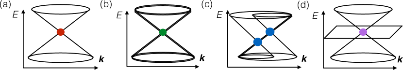
Figure 1: (a) Weyl points are twofold degenerate band crossings of two singly degenerate bands. (b) Dirac points are fourfold degenerate band crossings of two twofold degenerate bands. (c) Triple-points are threefold degenerate band crossings of a singly and a doubly degenerate band. Here a pair is shown. (d) A spin-1 generalization of a Weyl fermion [17].

2 Classification of Triple-Points

The realization of a symmorphic TP at a momentum $\bm{k}$ in the Brillouin zone (BZ) of a crystal structure requires the little group of $\bm{k}$ to contain both one- and two-dimensional double group representations, since both singly and doubly degenerate bands need to be present for the formation of the TP. Only the point group $C_{3v}$ satisfies these criteria, thus TPs appear on high-symmetry lines in the BZ with the little group $C_{3v}$. The elements of $C_{3v}$ are 3-fold rotation $C_{3}$ and 3 mirrors $\sigma_{v}$, containing the $C_{3}$ axis, rotated by 120 degrees relative to each other [23, 24, 25]. One notable exception from this rule is given by space group 174 ($C^{1}_{3h}$), where the interplay of time-reversal and mirror symmetry on a $C_{3}$-symmetric line also allows for both one- and two-dimensional double group representations.

Using the above symmetry criterion all space groups that can host TP fermions on a line are identified in Tab. 1. Note, that the little group on the high-symmetry axis of the type-B TP topological metals (TPTMs) is exactly $C_{3v}$, while for type-A TPTMs it is supplemented by an additional anti-unitary symmetry. This symmetry is the product of a mirror plane $\sigma_{h}$, orthogonal to the $C_{3}$-axis and time-reversal (TR). Its presence preserves the existence of doubly- and singly-degenerate representations, and, hence, allows for the existence of TPs. In our consideration we also included non-symmorphic space groups, such that the TP crossing includes the same irreducible representations as found in the symmorphic space groups.

Table 1: Space groups allowing for TPs of different types with time-reversal symmetry. The points can appear on high-symmetry lines in the Brillouin zone: $\Delta=(0,0,\alpha)$, $\Lambda=(\alpha,\alpha,\alpha)$, $P=(-1/3,2/3,\alpha)$ (hexagonal lattice), $P=(1/2-\alpha,1/2-\alpha,-1/2-\alpha)$ (rhombohedral lattice) and $F=(1/4+\alpha,1/4-3\alpha,1/4+\alpha)$. Triple-points appear in trigonal, hexagonal and cubic space groups. Note that the table contains also non-symmorphic space groups but the TPs exist on lines where the non-symmorphicity does not change the irreducible representations, thus they are identical to the TPs found in symmorphic space groups. The case of the non-symmorphic space group 220 has also been treated in Ref. [17]. We note that, in addition, the groups 162-167, 191-194 and 221-230 admit type-B TPs provided time-reversal symmetry is broken in a way preserving $C_{3v}$ representations on a line in the Brillouin zone.

TP type	$\Gamma$-A ($\Delta$) or $\Gamma$-P2 ($\Lambda$)	K-H ($P$) or P0-T ($P$)	$\Gamma$-L/R/P ($\Lambda$) or P-H ($F$)
type-A	174, 187-190
type-B	156-161	157, 159-161, 183-186, 189-190	215-220

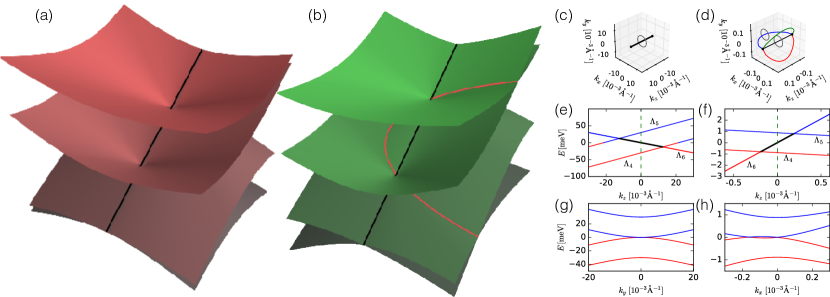
Figure 2: Two types of fermionic triple-point quasiparticles. (a) and (c) type-A triple-points are connected by a single nodal line, where conduction and valence bands are degenerate (shown in black). (b) and (d) type-B triple-points are accompanied by four such nodal lines, shown in black, green, blue and red. The latter three occur in the mirror-symmetric planes in momentum space. The grey circles in (c) and (d) indicate paths for the Berry phase calculation. (e)((f)) Band structure around a type-A (type-B) triple-point along the $C_{3}$ axis. Here $\Lambda_{6}$ represents the double degenerate band (double representation of $C_{3v}$), while $\Lambda_{4,5}$ correspond to two one-dimensional representations. The black lines in (e) and (f) mark the region of the band structure that produces the nodal lines shown in black in panels (c) and (d). (g)((h)) Band structure around a type-A (type-B) triple-point in a mirror symmetric plane orthogonal to $k_{z}$. The dashed green lines in (e) and (f) mark the momentum $k_{z}$ used in panels (g) and (h). Red (blue) color in panels (e-h) corresponds to occupied (unoccupied) bands assuming the Fermi level is exactly between the pair of triple-points. Figure partially reused from Ref. [21]

The topological classification of TPs into type-A and type-B stems from the different numbers of accompanying nodal lines, and also from the fact that the nodal lines accompanying the two types of TPs are topologically distinct. Due to the three vertical mirror planes, the Berry phase $\varphi_{\rm B}$ accumulated by valence bands on any mirror-symmetric path (shown in grey in Fig. 2(c-d)) enclosing the corresponding nodal line is quantized to be either $0$ or $\pi$ [26, 27]. The nodal line of type-A TPTMs has $\varphi_{\rm B}=0$, while all the lines of type-B TPs have $\varphi_{\rm B}=\pi$.

These values are consistent with the band structure plots, shown in Fig. 2(e-h). In type-A TPTMs the crossing of conduction and valence (occupied and unoccupied) bands occurs on a high-symmetry line and is quadratic, while for the type-B phase this quadratic touching point splits into two points, where the bands cross linearly. The presence of nodal lines with nontrivial Berry phase, as is the case for type-B, is generally associated with the appearance of surface states [28, 27]. The merging and subsequent annihilation of nodal lines is similar to the nexus point discussed in the context of ³He-A and Bernal-stacked graphite with neglected spin-orbit coupling (SOC) [29, 30, 31, 32]. We stress, however, that the scenarios discussed in the present work take full account of SOC.

Analogous to WPs [6], the minimal number of TPs in the BZ is four for materials preserving time-reversal symmetry. A pair of TPs located on a $C_{3v}$-symmetric line can be split into four WPs by lowering the $C_{3v}$ symmetry to $C_{3}$ (breaking $\sigma_{v}$), which can be achieved by a small Zeeman field parallel to the $C_{3}$ axis or by an atomic distortion. Conversely, imposing inversion symmetry onto the atomic structure makes the two TPs merge into a single DP. Hence, the TPTMs can be viewed as an intermediate phase separating Dirac and Weyl semimetals in materials with a $C_{3v}$-symmetric line in the BZ.

3 Triple-Point Materials

The possibility of new fermions in condensed matter systems sparked a huge effort in the first-principles community to look for suitable material candidates. While band structures with threefold degenerate crossings appear to be comparatively rare in nature, using extensive scans of material databases enabled by high-throughput calculations, a decent amount of material candidates for TPTMs could still be identified. Experimental investigations of some of these materials are currently under way with some results already published [33, 34, 35, 36, 37]. In Tab. 2 we list all TPTMs that have been predicted by first-principles methods up to the point of this writing.

Table 2: Theoretically predicted TPTMs classified in type-A and type-B. Material candidates for which experimental evidence of TPs exist are marked by an asterisk.

TP type	Material
type-A	MoC [21, 38], WC∗ [21, 33, 34], WN [21], ZrTe [21, 39], MoP∗ [21, 35, 36], MoN [21], TaN [21, 22], NbN [21], NbS [21], TaS [40], TaSb [41]
type-B	tensile strained HgTe [42], CuPt-ordered InAsSb∗ [20, 37], CuAgSe [43], LuPtBi [44], LuAuPb [44], YPtBi [44], GdPtBi [44], LuPtBi [44], LaPtBi [44]

The TPTMs have been predicted in three types of crystal structures: type-A TPTMs are exclusively of a tungsten carbide (WC) structure and type-B TPTMs either have cubic symmetry (HgTe, half-Heuslers) or are obtained by breaking the cubic $T_{d}$ symmetry to the subgroup $C_{3v}$ (tensile strained HgTe, CuPt-ordered InAsSb).

3.1 Triple-points in Tungsten Carbide like crystal structure

The type-A TPTM phase has been identified in a family of two-element metals AB (A={Zr, Nb, Mo, Ta, W}, B={C, N, P, S, Te}) listed in the type-A row of Tab. 2. These materials have a WC-type structure that belongs to space group $P\bar{6}m2$ ($D_{3h}^{1}$=187). The primitive unit cell, shown in Fig. 3(a), consists of two atoms A and B at Wyckoff positions 1a $(0,0,0)$ and 1d $(\frac{1}{3},\frac{2}{3},\frac{1}{2})$ respectively. The corresponding bulk BZ is shown in Fig. 3(b) along with the (001) and (010) surface BZs.

Figure 3: (a) Primitive unit cell of WC-type structure. (b) The bulk BZ and (001) and (010) surface BZs. Figure reused from Ref. [21].

Now we discuss the band structure obtained by ab initio simulations [21]. Fig. 4 shows the band structures of ZrTe, WC and TaN, which will be used as representative materials.

In the absence of SOC there is a band inversion at K and K’ points in ZrTe and WC (Fig. 4(a) and (c)), resulting in a nodal ring in the $k_{z}=0$ plane protected by $\sigma_{h}$, while this band inversion is absent in TaN. The common feature of all materials is that along the $C_{3v}$-symmetric $\Gamma$-A line there is a band crossing of a singly and doubly degenerate bands due to the inversion of the singly- ($\Lambda_{1}$) and the doubly-degenerate ($\Lambda_{3}$) states at A. This crossing produces a single no-SOC TP, and it is this feature that generates four TPs upon introducing SOC.

All the considered materials have sizable SOC, which cannot be neglected. Due to the lack of inversion symmetry the bands are spin-split at generic momenta as shown in Fig. 4(b,d,f). One finds a band inversion along the H-A-L line such that the A point acquires an inverted gap for all materials. Consequently, the $k_{z}=\pi$ plane becomes an analogue of a 2D quantum spin Hall insulator in all of the compounds. Topological confirmation of the presence of band inversion is given by the non-trivial values of the mirror Chern numbers [45] on the $\sigma_{h}$ planes, see Fig. 5, which are $C_{\pm i}=\mp 1$, for the mirror eigenvalues $\pm i$ respectively, in the $k_{z}=\pi$ plane for the materials considered here [21]. In the $k_{z}=0$ plane one finds $C_{\pm i}=\mp 1$ for ZrTe, MoP and NbS and $C_{\pm i}=0$ for MoN, TaN and NbN. The materials MoC, WC and WN have nodal lines in the $k_{z}=0$ plane and, therefore, the mirror Chern number is ill defined for them.

In ZrTe the nodal ring around K and K’ points acquires a small gap (see also the inset in Fig. 4(b)). Interestingly, three pairs of WPs, slightly away from the $k_{z}=0$ plane, form at each K and K’ point in ZrTe [39] and also in MoP [35]. WC (together with MoC and WN) remains a nodal line metal (see inset Fig. 4(d)). There exist two nodal rings (one inside another) formed by two touching bands protected by the horizontal mirror $\sigma_{h}$. For WN there is only a single such nodal ring around each $K$ and $K^{\prime}$. The stability of these topological features has been checked with the HSE06 hybrid functional [46, 21]. Furthermore, the band structure of MoP has been recently experimentally investigated using angle-resolved photoemission spectroscopy (ARPES), confirming experimentally the presence of TPs and WPs [35].

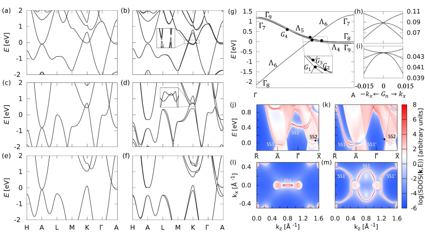
Figure 4: Band structure of ZrTe (a)((b)), WC (c)((d)), and TaN (e)((f)) without (with) SOC. The Fermi energy is set to 0 eV. (g) Band structure of ZrTe along the $\Gamma$-A line. Bands are labeled by their double group representations corresponding to $D_{3h}$ at $\Gamma$ and A points and $C_{3v}$ on the $\Gamma$-A line. (h)((i)) Band structures in the (100) direction with $k_{z}$ tuned to the TPs $G_{1}$ ($G_{2}$). (j) ((k)) Projected surface density of states (SDOS) for the (010) surface of ZrTe with Zr (Te) termination. (l)((m)) The (010)-surface Fermi surface of ZrTe at $E=0$ eV for Zr (Te) termination. Figure reused from Ref. [21].

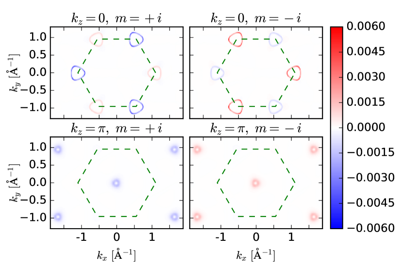
Figure 5: The Berry curvature for specific mirror eigenvalues on $\sigma_{h}$-mirror invariant planes in ZrTe. Figure reused from Ref. [21].

In Fig. 4(g) a zoom-in of the $\Gamma$-A line in ZrTe is shown. The Fermi level resides in between the $\Gamma_{9}$ and $\Gamma_{8}$ bands at A. Upon turning on the SOC the no-SOC $\Lambda_{3}$ state splits into the singly degenerate $\Lambda_{4}+\Lambda_{5}$ states and the doubly degenerate $\Lambda_{6}$ state. Another $\Lambda_{6}$ state comes from the no-SOC $\Lambda_{1}$. The two $\Lambda_{6}$ states hybridize and each of them crosses with the spin-split $\Lambda_{4,5}$ states creating 2 pairs of TPs: $(G_{1},G_{2})$ and $(G_{3},G_{4})$. Each TP is protected by the $C_{3v}$ symmetry of the $\Gamma$-A line. Fig. 4(h-i) shows the dispersion in the (100) direction for $k_{z}$ tuned to the position of $G_{1}$, $G_{2}$ respectively. A linear band crossing superimposed with a quadratic band resembles a WP, degenerate with a quadratic band, similar to the findings of Ref. [20] for type-B TPTMs. Again, band inversion is the mechanism leading to the formation of TPs.

In Fig. 4(j-k) the surface states of ZrTe for the (010) surface are shown [21, 47]. The surface potential is found to depend strongly on the termination choice: Zr (Te)-termination is shown in Fig. 4(j) (Fig. 4(k)). Since the $k_{z}=\pi$ plane is a quantum spin Hall insulator plane, a Kramers doublet of surface states should appear along the $\overline{\mathrm{A}}$-$\overline{\mathrm{R}}$ line of the surface BZ. Consequently, there is a surface Dirac cone SS1 located at $\overline{\mathrm{A}}$ ($\overline{\mathrm{R}}$) for Zr (Te) termination. The surface states forming the Dirac cone emerge from the TPs $G_{1}$ and $G_{2}$. For $k_{z}$ values below the location of $G_{1}$ and $G_{2}$, there exists another pair of surface states SS1’ emerging from the TPs. SS1’, however, is not topologically protected.

The K’ point of the bulk BZ is projected onto the $\overline{\Gamma}$-$\overline{\mathrm{X}}$ line in Fig. 4(j-k) (compare to Fig. 3(b)). A small gap due to SOC can be visible in the projected bulk spectrum around the projection of K point (shown with an arrow). For ZrTe the $k_{z}=0$ mirror plane hosts a quantum spin Hall phase with the mirror Chern numbers $\pm 1$, thus one can expect to see a Kramers pair of topological surface state along the line $\overline{\mathrm{X}}\leftarrow\overline{\Gamma}\rightarrow-\overline{\mathrm{X}}$. This expectation is further supported by the Berry curvature calculation in the $k_{z}=0$ plane, see Fig. 5. It reveals the accumulation of Berry curvature in an area around the K (K’) point that sums up to approximately $-1$ ($1$) [21]. In accord with this topological arguments one finds a quantum Hall like surface state SS2 crossing the gap along $\overline{\Gamma}$-$\overline{\mathrm{X}}$ (its Kramers partner is not shown, being at TR-symmetric part of the surface BZ.

Fig. 4(l-m) show the (010)-surface Fermi surface revealing double Fermi arcs between the two hole pockets containing the TPs, corresponding to SS1 and SS1’. The state SS2 is not visible for this choice of the Fermi level. For Te termination the Fermi arcs connect the two hole pockets, while they do not touch them for the Zr termination. In both cases, however, the surface states are protected by TR and mirror symmetry on the $k_{z}=\pi$ plane, so they can not be fully removed from the spectrum. ARPES investigations of the very similar TPTM WC prove the existence of the surface Fermi arcs SS1 and SS1’ [34].

3.2 Cubic symmetry

One of the first account of TPs has been given in the context of HgTe by Saad Zaheer et al. in Ref. [42]. According to the cubic symmetry there are eight equivalent directions with little group $C_{3v}$ hosting possible TPs. Due to the lack of a horizontal mirror these TPs are all of type-B. The situation is complicated by the fact that the $\Lambda_{4,5}$ and $\Lambda_{6}$ states are degenerate at $\Gamma$ forming the four-dimensional $\Gamma_{8}$ representation. This leads generically to eight TPs near a $\Gamma_{8}$ crossing along the eight equivalent $\Lambda$ directions, see Fig. 6 (a). However, in the HgTe case the TPs are extremely close to $\Gamma$ such that they are impossible to resolve with available experimental techniques.

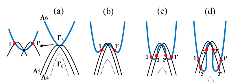
Figure 6: Energy bands along L-$\Gamma$-L in cubic crystalls with band inversion. The thick blue line is doubly degenerate whereas black lines are non-degenerate. (a) HgTe-type energy bands. (b-d) Evolution of band structure in half-Heusler materials with increasing number of TPs. Illustration adapted with permission from Ref. [44]

The same scenario takes place in half-Heusler compounds with band inversion [48]. Interestingly, in some compounds like LuPtBi, LuAuPb and YPtBi the energy bands have such a strong non-parabolicity that additional TPs appear [44]. The evolution of the band structure with increasing number of TPs is illustrated in Fig. 6 (b-d). Therefore these half-Heusler compounds have three TPs in each equivalent 111 direction, 24 in total. Furthermore, these TPs are well separated from the $\Gamma$ point with observable Fermi arcs on the easily cleavable (111) surface [44, 49, 50]. These properties make the half-Heusler compounds ideally suited to experimentally investigate the intricate topology and surface states of type-B TPs.

3.3 CuPt-ordered InAs_1-xSb_x

Above we have seen that the TPs of the cubic HgTe are too close to $\Gamma$ to enable a direct experimental observation. However, this can be changed by applying moderate tensile strain in the 111 direction, such that the remaining point group is broken down from $T_{d}$ to $C_{3v}$ [42]. In this case two pairs of TPs survive. Unfortunately, it is experimentally difficult to apply 111 strain to HgTe. The ingredients to achieve well separated TPs in HgTe are band inversion and breaking of cubic $T_{d}$ symmetry to $C_{3v}$. It is no surprise that the same ideas can be applied in other III-V semiconductors. The difficulty of applying 111 strain can be overcome by changing the mechanism of symmetry breaking from strain to alloy ordering. Fortunately, some ternary III-V compounds show naturally a so-called CuPt-ordering [51], which is ordering in alternating 111 planes, see Fig. 7 (a). This type of ordering provides exactly the desired symmetry breaking. Especially promising is the InAs_1-xSb_x system [20]. InAs and InSb are both small band gap semiconductors and the band gap is further reduced in their alloy [52, 53, 54]. CuPt-ordering further reduces the band gap [55, 51, 56] and first-principles calculations show that perfectly CuPt-ordered InAs_0.5Sb_0.5 alloy has an inverted band order [57, 20]. While perfect atomic CuPt-ordering in InAs_0.5Sb_0.5 is difficult to obtain the same effect is achieved by growing layered structures of InAs_1-xSb_x with alternating alloy composition $x$. With this approach the band gap can be tuned from normal to inverted band ordering [58, 37].

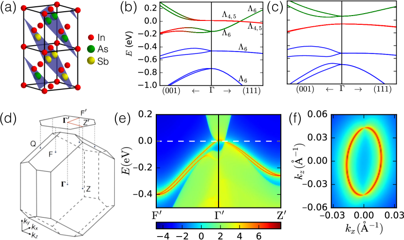
Figure 7: (a) Crystal structure of CuPt-ordered InAs_0.5Sb_0.5. (b) Band structure of CuPt-ordered InAs_0.5Sb_0.5 around $\Gamma$ (plotted up to $|{\bf k}|=0.1\,\mathrm{\AA}^{-1}$). (c) Band structure with 3% compressive strain applied in the 111-direction. (d) Brillouin zone and surface projection of CuPt-ordered InAs_0.5Sb_0.5. (e) Surface density of states for the $(1\bar{1}0)$ surface. (f) Topological Fermi arcs on the $(1\bar{1}0)$ surface. Figure partially reused from Ref. [20]

The band structure of CuPt-ordered InAs_0.5Sb_0.5 obtained from first-principles simulations is shown in Fig. 7(b) [20]. A pair of TPs is formed at the crossings of the $\Lambda_{4,5}$ with the $\Lambda_{6}$ band. The $\Lambda_{4,5}$ bands have a very small linear in $k$, splitting, which is only about 2 meV at the momentum of the TPs. The pair of TPs is thus very close together and will appear like a single Dirac point in low resolution experiments.

Another very interesting aspect of CuPt-ordered InAs_1-xSb_x is that the symmetry breaking to $C_{3v}$ simultaneously allows for a Rashba-type spin-orbit splitting in the conduction band, provided the band order is normal. Either by imperfect CuPt-ordering, or by 111 strain, the normal band order can be restored and one obtains a giant-Rashba material, see Fig. 7 (c). Large Rashba splitting is a crucial ingredient for topological quantum computers relying on non-abelian Majorana [59, 60, 61, 62, 63] quasiparticles realized in semiconductor nanowires [64, 65]. Since InAs and InSb are the preferred materials for the experimental realizations of Majorana quasiparticles [66, 67, 68, 69, 70], CuPt-ordered InAs_1-xSb_x seems to be a very promising material for this application [20].

Fig. 7 (e) and (f) shows the surface density of states of the $(1\bar{1}0)$ surface [20]. In this case the Fermi arcs resulting from the TPs look very similar to those from the typical Dirac semimetals [7, 8, 10] due to the small separation of the TPs.

4 Topological properties of Triple-Point Fermions

In this section we first introduce simplified models of TP materials and use them to discuss the topological properties of TPs.

4.1 Microscopic models

Before we investigate the topology of TPs we introduce a few simple ${\bm{k}}\cdot{\bm{p}}$-models for type-A and type-B triple-points. The type-A ${\bm{k}}\cdot{\bm{p}}$-models are up to a change of basis identical to the ones in Ref. [21] and the given parameters correspond to the material realization of ZrTe. The type-B ${\bm{k}}\cdot{\bm{p}}$-models are also up to a basis transformation identical to the ones in Ref. [20] and the parameters correspond to the CuPt-ordered InAs_0.5Sb_0.5 case.

4.1.1 Type-A: ZrTe

For the WC-class of type-A TPTMs we construct a model around the A point which captures the band inversion and describes the TPs. We include the $\Gamma_{9}$, $\Gamma_{8}$ and $\Gamma_{7}$ states (see Fig. 4 (g) and Tab. 65 of Ref. [23]) with energies close to the Fermi level. Along the $z$-axis the $\Gamma_{9}$ representations splits into the $\Lambda_{4,5}$ representations and both $\Gamma_{7,8}$ become $\Lambda_{6}$. The little group of A is $D_{3h}$ plus TR symmetry. For the derivation of the ${\bm{k}}\cdot{\bm{p}}$ models we need to identify the correct representations of the symmetry operations. The Hamiltonian is then constructed such that it commutes with all symmetries $S$

$$H(S({\bm{k}}))=R_{S}H({\bm{k}})R_{S}^{\dagger},$$ (1)

with $R_{S}$ being the representation of S in the basis of $H$. Since all representations are two dimensional the symmetry representation are the direct sum of two dimensional representations $R(\Gamma_{9})\oplus R(\Gamma_{7})\oplus R(\Gamma_{8})$,

$$C_{3} =\begin{pmatrix}-\frac{1}{2}&-\frac{\sqrt{3}}{2}\\ \frac{\sqrt{3}}{2}&-\frac{1}{2}\\ &&1\end{pmatrix},\ R_{C_{3}}=\mathrm{diag}(-1,-1,e^{-i\pi/3},e^{i\pi/3},e^{-i\pi/3},e^{i\pi/3}),$$ (2)

$$\sigma_{v} =\mathrm{diag}(-1,\phantom{-}1,\phantom{-}1),\ R_{\sigma_{v}}=\phantom{-}i\,\mathrm{diag}(\phantom{-}1,\phantom{-}1,\phantom{-}1)\otimes\tau_{x},$$

$$\sigma_{h} =\mathrm{diag}(\phantom{-}1,\phantom{-}1,-1),\ R_{\sigma_{h}}=\phantom{-}i\,\mathrm{diag}(\phantom{-}1,\phantom{-}1,-1)\otimes\tau_{z},$$

$$\mathrm{TR} =\mathrm{diag}(-1,-1,-1),\ R_{\mathrm{TR}}=-i\,\mathrm{diag}(\phantom{-}1,\phantom{-}1,\phantom{-}1)\otimes\tau_{y},$$

with $\tau_{x}$, $\tau_{y}$ and $\tau_{z}$ being the Pauli matrices.

Considering the constraint Eq. (1) for all symmetries above, one obtains the following Hamiltonian

$${\scriptsize H_{{\bm{k}}\cdot{\bm{p}}}^{\mathrm{A}}=\begin{pmatrix}\epsilon_{1}&Ak_{z}&E\left(k_{x}-ik_{y}\right)&0&0&D\left(-ik_{x}+k_{y}\right)\\ Ak_{z}&\epsilon_{1}&0&E\left(-k_{x}-ik_{y}\right)&D\left(ik_{x}+k_{y}\right)&0\\ E\left(k_{x}+ik_{y}\right)&0&\epsilon_{2}&0&-iBk_{z}&C\left(-ik_{x}-k_{y}\right)\\ 0&E\left(-k_{x}+ik_{y}\right)&0&\epsilon_{2}&C\left(ik_{x}-k_{y}\right)&-iBk_{z}\\ 0&D\left(-ik_{x}+k_{y}\right)&iBk_{z}&C\left(-ik_{x}-k_{y}\right)&\epsilon_{3}&0\\ D\left(ik_{x}+k_{y}\right)&0&C\left(ik_{x}-k_{y}\right)&iBk_{z}&0&\epsilon_{3}\end{pmatrix},}$$ (3)

using the definition $\epsilon_{i}({\bf k})=E_{i}+F_{i}(k_{x}^{2}+k_{y}^{2})+G_{i}k_{z}^{2}$ and ${\bm{k}}$ relative to the A point. Via fitting to the ZrTe band structure we obtain the following parameters for Eq. (3): $E_{1}=-0.0391$ eV, $E_{2}=1.3709$ eV, $E_{3}=0.0391$ eV, $F_{1}=3.75$ eVŲ, $F_{2}=-0.5$ eVŲ, $F_{3}=4.25$ eVŲ, $G_{1}=2.2$ eVŲ, $G_{2}=-12.64$ eVŲ, $G_{3}=1.5$ eVŲ, $A=0.17$ eVÅ, $B=0.24$ eVÅ, $C=2.9$ eVÅ, $D=0.054$ eVÅ and $E=2.76$ eVÅ.

If the influence of the $\Gamma_{7}$ state is removed one obtains a $4\times 4$ model

$${H_{{\bm{k}}\cdot{\bm{p}}}^{\mathrm{A,}4\times 4}=\begin{pmatrix}\epsilon_{1}&Ak_{z}&0&D\left(-ik_{x}+k_{y}\right)\\ Ak_{z}&\epsilon_{1}&D\left(ik_{x}+k_{y}\right)&0\\ 0&D\left(-ik_{x}+k_{y}\right)&\epsilon_{3}&0\\ D\left(ik_{x}+k_{y}\right)&0&0&\epsilon_{3}\end{pmatrix}.}$$ (4)

To simulate the interaction of the two $\Lambda_{6}$ bands we add a fourth order term to $\epsilon_{3}({\bf k})=E_{3}+F_{3}(k_{x}^{2}+k_{y}^{2})+G_{3}k_{z}^{2}+H_{3}k_{z}^{4}$. We found the following parameters via fitting to the band structure of ZrTe: $E_{1}=-0.0391$ eV, $E_{3}=0.0391$ eV, $F_{1}=4.5$ eVŲ, $F_{3}=-7.3$ eVŲ, $G_{1}=2.2$ eVŲ, $G_{3}=3.2$ eVŲ, $H_{1}=0$ eVÅ⁴, $H_{3}=-20$ eVÅ⁴, $A=0.17$ eVÅ and $D=0.487$ eVÅ. Note that the parameter A is the only one that breaks inversion symmetry in the above model. Setting $A=0$ one obtains a ${\bm{k}}\cdot{\bm{p}}$ description of a Dirac semimetal.

A four band Hamiltonian in the vicinity of a pair of TPs, where ${\bm{k}}$ is understood relative to the midpoint of the two TPs is given below

$${H_{{\bm{k}}\cdot{\bm{p}}}^{\mathrm{TP}_{\mathrm{A}}}=\begin{pmatrix}A_{1}k_{z}&A_{2}k_{z}+E_{0}&iD\left(k_{x}-ik_{y}\right)&iC\left(k_{x}+ik_{y}\right)\\ A_{2}k_{z}+E_{0}&A_{1}k_{z}&iC\left(k_{x}-ik_{y}\right)&iD\left(-k_{x}-ik_{y}\right)\\ -iD\left(k_{x}+ik_{y}\right)&-iC\left(k_{x}+ik_{y}\right)&Bk_{z}&0\\ -iC\left(k_{x}-ik_{y}\right)&-iD\left(-k_{x}+ik_{y}\right)&0&Bk_{z}\end{pmatrix}.}$$ (5)

Instead of $\sigma_{h}$ and TR only their product $\theta\circ\sigma_{h}$ needs to be taken into account at a general ${\bm{k}}$-point on the $C_{3v}$-symmetric $z$-axis. In the following we used $E_{0}=30\,\mathrm{meV}$, $A_{1}=1.4\,\mathrm{eV\AA}$, $A_{2}=0\,\mathrm{eV\AA}$, $B=-1.0\,eV\mathrm{\AA}$, $C=1.082\,eV\mathrm{\AA}$ and $D=0\,\mathrm{eV\AA}$. We use above ${\bm{k}}\cdot{\bm{p}}$ model for the illustrations of the type-A TPTM in Fig. 2.

The WC-class of TPTMs also has interesting topological properties around the K-points. A good ${\bm{k}}\cdot{\bm{p}}$ description of the topology and bands around K (or K’) requires at least 8 states. The little group of the K points is $C_{3h}$ and the $\Gamma_{7}$, $\Gamma_{12}$, $\Gamma_{11}$, $\Gamma_{9}$, $\Gamma_{12}$, $\Gamma_{10}$, $\Gamma_{8}$ and $\Gamma_{7}$ states (see Tab. 57 of Ref. [23]) are determined to be relevant for constructing a ${\bm{k}}\cdot{\bm{p}}$-description. We use the following symmetry representations

$$C_{3} =\begin{pmatrix}-\frac{1}{2}&-\frac{\sqrt{3}}{2}\\ \frac{\sqrt{3}}{2}&-\frac{1}{2}\\ &&1\end{pmatrix},R_{C_{3}}=\mathrm{diag}(e^{i\frac{\pi}{3}},-1,-1,e^{i\frac{\pi}{3}},-1,e^{-i\frac{\pi}{3}},e^{-i\frac{\pi}{3}},e^{i\frac{\pi}{3}}),$$ (6)

$$\sigma_{h} =\mathrm{diag}\{\phantom{-}1,\phantom{-}1,-1\},R_{\sigma_{h}}=\mathrm{diag}(i,-i,i,-i,-i,i,-i,i).$$

Considering the symmetries given above, the lowest order Hamiltonian around K is given by

$${H_{{\bm{k}}\cdot{\bm{p}}}^{\mathrm{K}}=\begin{pmatrix}\epsilon_{1}&0&B_{1}\,k^{+}&A_{1}\,k_{z}&0&B_{3}\,k^{-}&0&0\\ 0&\epsilon_{2}&-A^{\prime}_{1}\,k_{z}&B_{2}\,k^{-}&0&0&B_{4}\,k^{+}&0\\ B_{1}^{*}\,k^{-}&-A^{\prime*}_{1}\,k_{z}&\epsilon_{3}&0&A_{2}\,k_{z}&B_{9}\,k^{+}&0&B_{5}\,k^{-}\\ A_{1}^{*}\,k_{z}&B_{2}^{*}\,k^{+}&0&\epsilon_{4}&-B^{\prime}_{9}\,k^{+}&0&B_{6}\,k^{-}&A_{4}\,k_{z}\\ 0&0&A_{2}^{*}\,k_{z}&-B^{\prime*}_{9}\,k^{-}&\epsilon_{5}&0&B_{7}\,k^{+}&0\\ B_{3}^{*}\,k^{+}&0&B_{9}^{*}\,k^{+}&0&0&\epsilon_{6}&A_{3}\,k_{z}&B_{8}\,k^{+}\\ 0&B_{4}^{*}\,k^{-}&0&B_{6}^{*}\,k^{+}&B_{7}^{*}\,k^{-}&A_{3}^{*}\,k_{z}&\epsilon_{7}&0\\ 0&0&B_{5}^{*}\,k^{+}&A_{4}^{*}\,k_{z}&0&B_{8}^{*}\,k^{-}&0&\epsilon_{8}\end{pmatrix},}$$ (7)

using $\epsilon_{i}$ defined as in Eq. (3), $k^{\pm}=k_{x}\pm ik_{y}$ and ${\bm{k}}$ relative to K. Since K is not a time-reversal invariant momentum bands do not form doubly degenerate Kramers pairs at this point. For the ${\bm{k}}\cdot{\bm{p}}$ model around the K point we obtain the following parameters (in units of eV and Å) via fitting to the ZrTe band structure: $E_{1}=-0.0979$, $E_{2}=-0.0671$, $E_{3}=0.6538$, $E_{4}=0.8393$, $E_{5}=1.0661$, $E_{6}=1.1351$, $E_{7}=1.2145$, $E_{8}=1.2774$, $F_{1}=F_{2}=3.6$, $F_{3}=F_{4}=-2.0$, $F_{5}=F_{6}=6.0$, $F_{7}=F_{8}=1.5$, $G_{1}=G_{2}=3.6$, $G_{3}=G_{4}=-0.2$, $G_{5}=G_{6}=2.0$, $G_{7}=G_{8}=-3.0$, $A_{1}=A^{\prime}_{1}=4.0$, $A_{2}=0.2$, $A_{3}=0$, $A_{4}=0$, $B_{1}=0.2-i0.1$, $B_{2}=0.02-i0.01$, $B_{3}=0.2$, $B_{4}=-0.2$, $B_{5}=-1.0+i4.0$, $B_{6}=-4.0+i1.0$, $B_{7}=3.0+i0.5$, $B_{8}=-0.5+i3.0$ and $B_{9}=1.5$. The Weyl points reported in Ref. [39] are also described by this ${\bm{k}}\cdot{\bm{p}}$ model.

4.1.2 Type-B: CuPt-ordered InAs_0.5Sb_0.5

The type-B scenario differs only by the absence of the horizontal mirror $\sigma_{h}$. For completenes we give the corresponding representations again, albeit $\sigma_{v}$ is now a mirror in the $xz$-plane instead of the $xy$-plane as before. The representations below correspond to a $\Lambda_{4,5}\oplus\Lambda_{6}$-basis

$$C_{3} =\begin{pmatrix}-\frac{1}{2}&-\frac{\sqrt{3}}{2}\\ \frac{\sqrt{3}}{2}&-\frac{1}{2}\\ &&1\end{pmatrix},\ R_{C_{3}}=\mathrm{diag}(-1,-1,e^{-i\pi/3},e^{i\pi/3}),$$ (8)

$$\sigma_{v} =\mathrm{diag}(\phantom{-}1,-1,\phantom{-}1),\ R_{\sigma_{v}}=\phantom{-}i\,\mathrm{diag}(\phantom{-}1,\phantom{-}1)\otimes\tau_{y},$$

$$\mathrm{TR} =\mathrm{diag}(-1,-1,-1),\ R_{\mathrm{TR}}=-i\,\mathrm{diag}(\phantom{-}1,\phantom{-}1,\phantom{-}1)\otimes\tau_{y},$$

Around $\Gamma$ the following model is obtained

$${H_{{\bm{k}}\cdot{\bm{p}}}^{\mathrm{B}}=\begin{pmatrix}\epsilon_{1}&-iAk_{z}&iB_{1}\left(k_{x}-ik_{y}\right)&iB_{2}\left(k_{x}+ik_{y}\right)\\ iAk_{z}&\epsilon_{1}&iB_{2}\left(k_{x}-ik_{y}\right)&iB_{1}\left(-k_{x}-ik_{y}\right)\\ -iB_{1}\left(k_{x}+ik_{y}\right)&-iB_{2}\left(k_{x}+ik_{y}\right)&\epsilon_{2}&iC\left(k_{x}-ik_{y}\right)\\ -iB_{2}\left(k_{x}-ik_{y}\right)&-iB_{1}\left(-k_{x}+ik_{y}\right)&-iC\left(k_{x}+ik_{y}\right)&\epsilon_{2}\end{pmatrix},}$$ (9)

with the following set of parameters for CuPt-ordered InAs_0.5Sb_0.5: $E_{1}=0.1696$ eV, $E_{2}=0$ eV, $F_{1}=-5.86$ eVŲ, $F_{2}=14.3$ eVŲ, $G_{1}=-3.91$ eVŲ, $G_{2}=54.2$ eVŲ, $A=0.02$ eVÅ, $B_{1}=0$,$B_{2}=1.48$ eVÅ and $C=1.26$ eVÅ.

Omitting the TR symmetry, a Hamiltonian of a pair of TPs, with ${\bm{k}}$ relative to the midpoint of the two TPs, is obtained

$${H_{{\bm{k}}\cdot{\bm{p}}}^{\mathrm{TP}_{\mathrm{B}}}=\begin{pmatrix}A_{1}k_{z}&-i\left(A_{2}k_{z}+E_{0}\right)&F\left(k_{x}-ik_{y}\right)&D\left(k_{x}+ik_{y}\right)\\ i\left(A_{2}k_{z}+E_{0}\right)&A_{1}k_{z}&D\left(-k_{x}+ik_{y}\right)&F\left(k_{x}+ik_{y}\right)\\ F^{*}\left(k_{x}+ik_{y}\right)&D^{*}\left(-k_{x}-ik_{y}\right)&Bk_{z}&C\left(ik_{x}+k_{y}\right)\\ D^{*}\left(k_{x}-ik_{y}\right)&F^{*}\left(k_{x}-ik_{y}\right)&C\left(-ik_{x}+k_{y}\right)&Bk_{z}\end{pmatrix}.}$$ (10)

In contrast to Eq. (5) the parameters $D$ and $F$ can now take complex values. We use $E_{0}=0.88$ meV, $A_{1}=-0.42$ eVÅ, $A_{2}=0$ eVÅ, $B=4.22$ eVÅ, $C=0.78$ eVÅ, $D=0.755-0.445i$ and $F=-1.69+0.755i$. We use above ${\bm{k}}\cdot{\bm{p}}$ model for the illustrations of the type-B TPTM in Fig. 2.

4.2 Wilson loop characterization for pairs of triple-points

The tracking of Wilson loop eigenvalues [71], or equivalently the so-called hybrid Wannier centers [72], under an adiabatic modification of a Hamiltonian has been proven as an invaluable tool for classifying topological phases [73, 74, 11, 75]. Here a $\mathbb{Z}_{2}$ topological classification based on the Wilson loop is developed for pairs of TPs.

The Wilson loop can be defined on any path in $k$-space connecting two points ${\bf k_{1}}$ and ${\bf k_{2}}$ with the property ${\bf k_{1}}={\bf k_{2}}+{\bf G}$, where ${\bf G}$ is a reciprocal lattice vector. The Wilson loop is defined as the path ordered product [71]

$$\mathcal{W}_{\bf k_{1}k_{2}}=P_{\bf k_{1}}\left(\prod_{j=1,2,\dots}P_{\bf k^{\prime}_{j}}\right)P_{\bf k_{2}},$$ (11)

with $P_{\bf k}=\sum_{n\in\mathrm{occ.}}|u_{n}({\bf k})\rangle\langle u_{n}({\bf k})|$ the projector on the occupied subspace of a Hamiltonian. The Wilson loop is inherently gauge invariant due to the gauge invariance of the projector $P_{\bf k}$. The Berry phase associated with the loop is given by the determinant of the Wilson operator $\det(\mathcal{W})=\exp(i\phi_{B})$. If the Hamiltonian has a symmetry $R$, it can be shown that [76]

$$\tilde{R}\mathcal{W}_{\bf k_{1}k_{2}}\tilde{R}^{-1}=\mathcal{W}_{R{\bf k_{1}}R{\bf k_{2}}},$$ (12)

with $R$ acting in reciprocal space and $\tilde{R}$ in occupied band space. The symmetry expectation value of Wilson loop eigenstates $|v_{i}\rangle$ is calculated as $\langle v_{i}|\tilde{R}|v_{i}\rangle$.

For Weyl [11] and Dirac [75] semimetals it is known that the Wilson loop spectrum on a sphere enclosing the semimetallic point gives the topological classification of the crossing. Also in our case with TPs a similar kind of topological classification is possible. Here the classification is demonstrated with a tight-binding model of ZrTe obtained in Ref. [21].

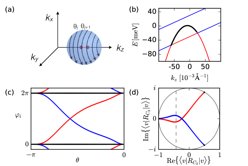
Figure 8: (a) Pair of TPs (red points) connected by a nodal line (red line) enclosed by a sphere. The arrows indicate the individual Wilson loops winding around the sphere. (b) Example of a trivial pair of TPs. (c) The Wilson loop spectrum on a sphere enclosing a pair of TPs. Two Wilson loop eigenvalues feature gapless flow (colored in red and blue). (d) $C_{3}$ symmetry expectation value of individual Wilson lines. Figure reused from Ref. [21].

In Fig. 8(a) we show a spherical surface on which the Wilson loop spectrum is to be evaluated. The sphere is chosen such that the Hamiltonian is gapped everywhere on the surface, the symmetry axis containing the TPs goes through the center of the sphere and both TPs are enclosed by the sphere. The latter point is important, since there is always at least one nodal line connecting two TPs, therefore including only one TP would not fulfill the requirement that the Hamiltonian is gapped on the sphere. Note that the Wilson lines are oriented such that the symmetry axis goes through their center. In Fig. 8(c) we plot the phases $\phi_{i}$ of the individual Wilson loop eigenvalues as a function of the azimuthal angle $\theta$. The tight-binding model has 8 occupied states, therefore, we obtain 8 Wilson loop eigenvalue phases $\phi_{i}$. 6 $\phi_{i}$ (marked in black) are trivial and stay very close to 0 ($2\pi$), but two (marked in red and blue) seem to cross. Note that the $\sigma_{v}$ symmetry constrains the $\phi_{i}$ such that the Wilson loop spectrum is mirror symmetric $\phi_{i}=-\phi_{j}$ [26]. Since the Hamiltonian is gapped on the surface, and the Wilson loop is gauge invariant, the individual $\phi_{i}$ change smoothly with $\theta$. Therefore, the connectivity of the $\phi_{i}$ can be determined as long as they are not degenerate. To obtain the connectivity across the degeneracy point between the red and blue Wilson eigenvalues we calculate the $C_{3}$ symmetry expectation values of the corresponding states in Fig. 8(d). The grey dashed line in Fig. 8(d) indicates the position of the crossing of the blue and red line in Fig. 8(c). Note that the crossing of red and blue lines in Fig. 8(d) is accidental and we found that it can be avoided via choosing a cigar-shape, rather than a sphere. However, the $C_{3}$ symmetry expectation value is nondegenerate at the crossing Fig. 8(c) and we can use Fig. 8(d) to unambiguously determine the connectivity for all $\theta$. Therefore, the red and blue lines in the Wilson loop spectrum clearly indicate two hidden Berry curvature fluxes, one inward and one outward, through the sphere. The fluxes can be separated in the Wilson loop eigenbasis, corresponding to individual Chern numbers [77] of $\pm 1$. The difference of the two individual Chern numbers divided by two constitutes a $\mathbb{Z}_{2}$ topological invariant for TPs.

At the polar regions $\theta\approx 0$ or $\theta\approx-\pi$ the Wilson loop commutes with the $C_{3}$ symmetry due to Eq. (12). In this case the $C_{3}$ expectation value in Fig. 8(d) is one of the possible $C_{3}$ eigenvalues $\{-1,\exp(i\pi/3),\exp(-i\pi/3)\}$, which are the starting and ending points of the lines in Fig. 8(d). Note that the 6 trivial $\phi_{i}$ (black dots) are almost fixed to the $C_{3}$ eigenvalues, whereas the two nontrivial $\phi_{i}$ (red/blue dots) change the $C_{3}$ eigenvalue from $\{-1,\,-1\}$ to $\{\exp(i\pi/3),\,exp(-i\pi/3)\}$. Responsible for this behaviour are the two valence bands having the rotational eigenvalues $-1,\,-1$ for $k_{z}$ to the left of the two TPs and $\exp(i\pi/3),\,exp(-i\pi/3)$ for $k_{z}$ to the right of the two TPs. Therefore, the planes above $G_{1},\,G_{2}$ are topologically distinct from the planes below, consequently uncovering the existence of crossing points realized as the two TPs here.

In Fig. 8(b) we give an example of a topologically trivial pair of TPs. In this case the $C_{3}$ eigenvalues of the valence bands are the same to the left and to the right of the two TPs and hence the Wilson loop spectrum is in general gapped with an even $\mathbb{Z}_{2}$ invariant.

4.3 Lifshiftz transitions

Using the models of Eq. (5) and (10) we can analyze the Lifshitz transitions of Fermi surfaces in the TPTMs. The nodal lines of Fig. 2(a-b) guarantee that several Fermi surfaces touch within a finite energy window in between two TPs. Fig. 9(a) illustrates the fixed $k_{y}=0$ cuts of the Fermi surface for the Fermi level $E_{\rm F}$ placed above, below and in between the two TPs, representing three topologically distinct Fermi surfaces. At each of the two TPs a topological Lifshitz transition takes place: one of the Fermi pockets shrinks to a point reopening either inside or outside another Fermi pocket. When the $E_{\rm F}$ is placed in between the two TPs there appears a topologically protected touching point between electron and hole pockets, similar to the type-II WP scenario [11].

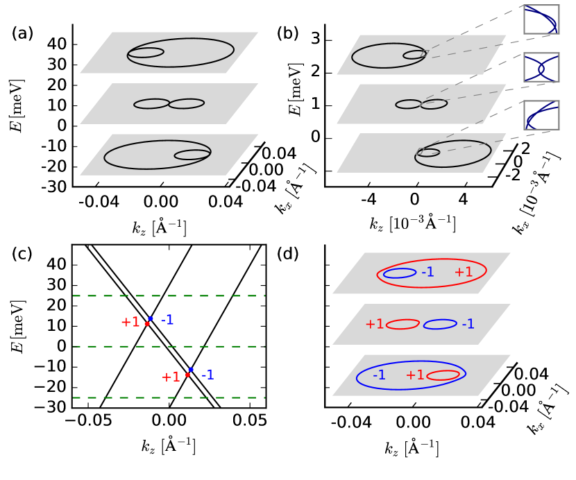
Figure 9: (a)((b)) Fermi surfaces for type-A (type-B) triple-point topological metals at three different energy cuts: below, between and above the two triple-points. The three small insets in panel (b) show that for the type-B scenario there are several distinct touching points between the Fermi pockets. (c) Band structure around the triple-points for a small Zeeman field parallel to the $C_{3}$ axis. (d) Fermi surface of type-A triple-point topological metal with a small Zeeman field. In panel (c) and (d) the Chern numbers of WPs and Fermi surfaces are marked in red ($+1$) and blue ($-1$). Figure reused from Ref. [21].

The Lifshitz transitions occurring in type-B TPTMs are illustrated in Fig. 9(b). The difference to the type-A transitions is that a single touching point between the Fermi pockets (the point of quadratic band touching) now splits into four points (or two linear band touchings on each mirror plane) due to the breaking of $\sigma_{h}$ (see insets of Fig. 9(b)). Intricate spin textures with changing winding numbers, were predicted for a (111)-strained HgTe in Ref. [42], which according to the classification is a type-B TPTM. Nontrivial windings in the spin-texture are also found for type-A TPTMs [22].

Since the distinct Fermi pockets touch in TPTMs for a range of energies, the topological charge of individual pockets is undefined. However, as mentioned above, this degeneracy is lifted by breaking $\sigma_{v}$ by, for example, applying a small Zeeman field in the $z$ direction or photoirradiation effects [78]. In this case each of the TPs splits into two WPs with opposite Chern numbers as illustrated in Fig. 9(c). The touching Fermi pockets now separate, and well-defined Chern numbers can be assigned to each of them, see Fig. 9(d). The Chern number of a pocket is equal to the summed up chiralities of WPs enclosed within it.

4.4 Surface states

Here we use the previously defined ${\bm{k}}\cdot{\bm{p}}$ models to gain insights into the first principles surface states shown in Sec. 3. The ${\bm{k}}\cdot{\bm{p}}$ surface state calculations are faciliated by discretizing the momentum perpendicular to the surface, and thus generating a 1D tight-binding model with the parallel momenta as auxilliary parameters [79]. The SDOS is then calculated using the iterative Green’s function method [80, 81]. For the ${\bm{k}}\cdot{\bm{p}}$ models given in Eq. (3) and (4) we use 1 Å as the discretization length and 2 Å for Eq. (7).

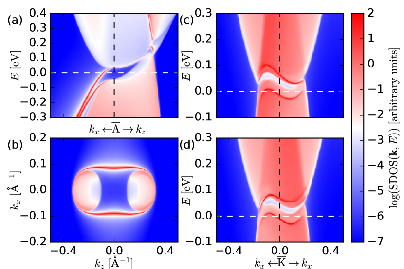
Figure 10: SDOS of the (010)-surface for the ${\bm{k}}\cdot{\bm{p}}$ models given in Eq. (3) and (7). (a) and (b) show the SDOS and Fermi surface around the $\overline{\mathrm{A}}$ point. (c) ((d)) show the SDOS around the $\overline{\mathrm{K}}$ point for the top (bottom) surface. Figure reused from Ref. [21].

We use the ${\bm{k}}\cdot{\bm{p}}$ models with parameters such that they fit the band structure of ZrTe. The model around A, given in Eq. (3), is characterized by the mirror Chern numbers $C_{m=\pm i}=\mp 1$ in the $k_{z}=\pi$ plane. Therefore, a topological-insulator-like surface state is expected on a surface orthogonal to the $\sigma_{h}$ mirror plane. In Fig. 10(a) we show the SDOS on a surface orthogonal to $y$, corresponding to the (010) surface in the WC structure. On the $k_{x}$ axis the upper topologically nontrivial surface state emerges from the conduction bands and connects to the valence bands. There is another trivial surface state with opposite mirror eigenvalue below. If we compare this to the first-principles surface states shown in Fig. 4(k) then these two surface states will form a Dirac cone at $\overline{\mathrm{R}}$ for Te-terminated surface. In Fig. 10(b) the Fermi surface is plotted. The topologically nontrivial hole pockets are connected by a pair of Fermi arcs.

The ${\bm{k}}\cdot{\bm{p}}$ model around K is characterized by a total Chern number of $C=1$, respectively $C=-1$ at K’. Hence around K and K’ a quantum Hall like surface state is expected. This is confirmed in Fig. 10(c) and (d), where we calculated the SDOS on a surface orthogonal to $y$. The surface states give an excellent match to the first principles result presented in Fig. 4 (j-k).

We now want to take a closer look at the surface states of TPs. Generally, one can distinguish two different scenarios. The first one corresponds to a pair of TPs that is very close together, i.e. the inversion symmetry breaking is small. Then one cannot discriminate which of the two TPs is the source of a Fermi arc and consequently the Fermi arcs have the characteristics of a Dirac semimetal like in the CuPt-ordered InAs_0.5Sb_0.5 case, see Fig. 7 (f) [20]. In the other scenario, one deals with isolated or a well separated pair of TPs. Here it is more useful to consider each TP as two degenerate Weyl nodes with opposite chirality, see Fig. 9 (c). In this case it is natural that each TP has two Fermi arcs connecting with their neighbors (it is also possible that the two WPs themselves are connected by a Fermi arc which vanishes when they form a TP) [44]. This scenario corresponds to the TPs in WC-like structures and in half-Heuslers.

It is insightful to look at the evolution of Fermi arcs from Dirac semimetal to TPTM. In a ${\bm{k}}\cdot{\bm{p}}$-model for ZrTe proposed in Ref. [21] one can easily tune between inversion symmetric and asymmetric band structures. In Fig. 11 we compare the surface states obtained from this model with and without inversion symmetry. In the presence of inversion and TR symmetry the two TPs merge into a four-fold degenerate Dirac point. Across all energies in the gap the two hole pockets around $\overline{\mathrm{A}}$ are connected by two Fermi arcs and the surface state on the $k_{z}$-axis is two-fold degenerate. Breaking of inversion symmetry then splits the Dirac point into two TPs. Each TP contributes a single non-degenerate surface state. Since the two surface states are split along the $k_{z}$-axis, the Fermi arcs are not required to connect the two hole pockets. Instead, one finds a topological-insulator-like Dirac cone around $\overline{\mathrm{A}}$ which is still protected by TR and $\sigma_{h}$ symmetries.

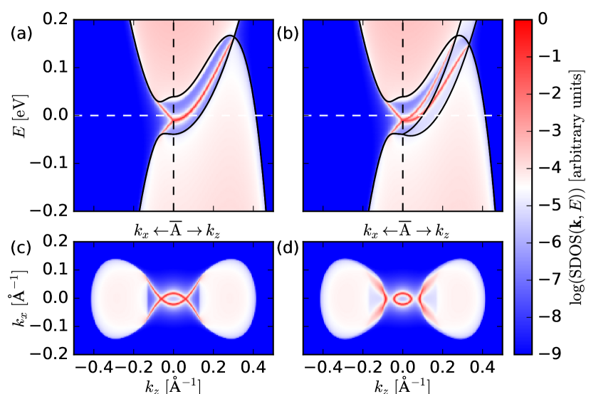
Figure 11: Surface states on the (010)-surface obtained from a ${\bm{k}}\cdot{\bm{p}}$ model for ZrTe Eq. (4). (a) ((b)) shows the surface density of states (the black lines show the bulk dispersion for $k_{y}=0$) and (c) ((d)) the surface Fermi surface with (without) inversion symmetry. Figure reused from Ref. [21].

4.5 Magnetotransport

The topologically non-trivial nature of Weyl semimetals reveals itself most spectacularly in the so-called chiral anomaly of the quantum field theory, realized by negative magnetoresistance [82, 83, 29, 84, 85, 86]. Type-I WPs produce a gapless Landau level spectrum in a magnetic field, whereas Type-II WPs have an anisotropic chiral anomaly [11], where the Landau level spectrum is gapless only for certain directions of the applied magnetic field.

The magnetotransport properties of TPs also depend on the direction of an applied magnetic field. A $C_{3}$ preserving magnetic field (along the $C_{3}$-axis) does not gap the Landau level spectrum of a TP, but instead each TP contributes a single chiral Landau level. However, if the field is applied in a $C_{3}$-breaking direction the Landau level spectrum becomes gapped. Such a direction dependence also occurs in Dirac semimetals [87].

The Landau levels are obtained by performing a Peierls substitution of $k_{x}$ and $k_{y}$ in the ${\bm{k}}\cdot{\bm{p}}$ Hamiltonian by $k_{x}=\frac{i}{\sqrt{2}l_{B}}(a^{\dagger}-a)$ and $k_{y}=\frac{i}{\sqrt{2}l_{B}}(a^{\dagger}+a)$, with $l_{B}=\sqrt{\frac{\hbar}{eB}}$ the magnetic length and $a^{\dagger}$, $a$ the raising and lowering operators $a^{\dagger}|n\rangle=\sqrt{n+1}|n+1\rangle$ and $a|n\rangle=\sqrt{n}|n-1\rangle$. In Fig. 12 we show the Landau level spectrum of CuPt-ordered InAs_0.5Sb_0.5 and ZrTe [20, 21]. When the magnetic field is turned on a pair of TPs turns into two crossing chiral Landau levels with opposite chirality. Due to the gapless Landau level spectrum strong signatures of the TPTM state are observable in magnetotransport. Analog to the chiral anomaly one can create a $\mathbb{Z}_{2}$ anomaly by applying parallel magnetic and electric field [88].

Magnetotransport experiments in the TPTM WC confirm the presence of direction dependent negative magnetoresistance for parallel magnetic and electric field [33]. Due to material growth constraints the longitudinal magnetoresistance has been only measured in directions orthogonal to the 001 axis. Further investigations are required to confirm that the negative magnetoresistance stems from the TPs.

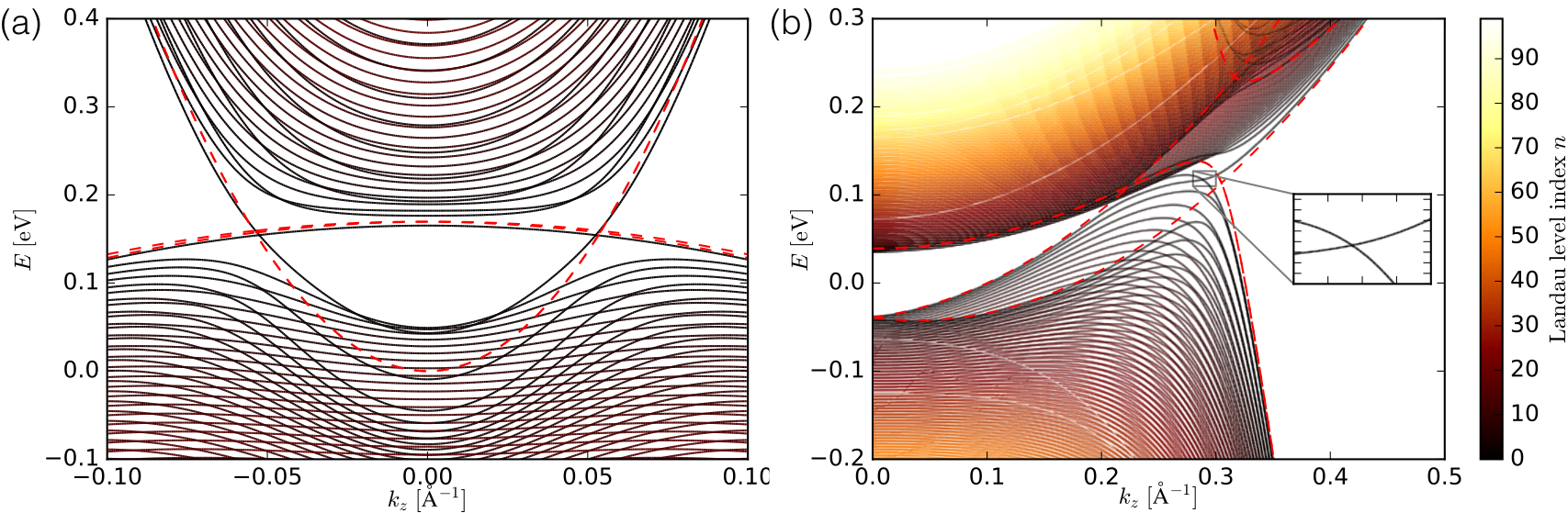
Figure 12: (a) ((b)) Landau levels in CuPt-ordered InAs_0.5Sb_0.5 (ZrTe) for a magnetic field of 50 (20) Tesla applied parallel to the $C_{3}$ axis using the $kp$-model of Eq. (9) (Eq. (3)). The dashed red lines show the bulk bands. Figure adapted from Refs. [20, 21].

5 Topology of phonons in triple-point metals

After describing the topological electronic properties of triple-point metals, we shift our focus to the topological vibrational properties of these compounds. The concept of topology from the electronic bandstructure has been successfully extended to the vibrational bandstructure of materials [89, 90, 91, 92, 93]. In recent works, topologically protected band-crossings have been reported in the phonon spectrum of solid state crystals [94, 95, 96, 41, 97]. Soon after the theoretical prediction of double-Weyl phonons in the phonon spectrum of transition-metal monosilicides $M$Si ($M$=Fe, Co, Mn, Re, Ru) [94], Miao et al. [98] experimentally reported the first observation of double Weyl points in FeSi by means of inelastic x-ray scattering measurements. This paved the way for realization of novel phononic (bosonic) quasiparticle excitations and the associated topological properties in condensed matter systems. Several other studies focused on the topology of phonons in model systems, and predicted novel quantum phenomena arising due to the non-trivial topology of phonons, such as quantum Hall conductance, quantized phonon Berry phase, topologically protected pseudo spin-polarized interface states, phonon pseudospin Hall effect, valley effects of phonons, realization of phonon diode, and topological acoustics [99, 100, 101, 102, 103, 104, 105, 106, 107, 108, 109]. Recently, topologically protected Weyl nodal lines have been predicted in the phonon spectrum of bulk MgB₂ [97].

Analogous to the physics of the electronic bandstructure, a nontrivial band-inversion between the low frequency acoustic and high frequency optical phonon modes results in topologically protected phonon band-crossings in the momentum space. Low frequency excitations of phonons near these topological band-crossing points could yield features of novel bosonic quasiparticles, such as Dirac, Weyl, and/or triple-point. Here, one main difference from the electronic structure stems from the fact that phononic excitations have bosonic character, whereas low-energy electronic excitations are fermionic. This rules out the applicability of the Pauli’s exclusion principle on phononic excitations in crystalline solids. In addition to the crystalline systems, topological bosonic quasiparticles have been realized in the photonic systems, metamaterials, and optical lattices [110, 111, 112, 113, 114, 115, 116, 117, 118, 119]. Moreover, Süsstrunk and Huber reported that oscillations of simple pendulum in classic mechanical systems could also host topological bosonic modes [91, 92, 93].

Although Dirac and Weyl phonon modes have been known since the last decade [120], triple-point phonons joined the family of topological phonons only in 2018 [96, 41]. In Refs. [96, 41], the existence of triple-point phonons was predicted in several special type-A triple-point metals having $C_{3v}$ symmetry, such as ZrTe, HfTe, TiS, TaSb, and TaBi. Notably, these materials also host Weyl fermions and triple-point fermions in their electronic spectrum. These binary compounds belong to space group #187 ($P\bar{6}m2$ ) having 2 atoms in the primitive cell and thus, inheriting three acoustic and three optical branches in their phonon spectrum. When the mass difference ($\Delta m=M-m$, where $M>m$) between the constituent atoms is large, the direct frequency band gap between the optical and acoustic branches ($\Delta_{g}$) is finite and positive at the A(0, 0, $\frac{\pi}{c}$) point of the hexagonal Brillouin zone. With decreasing $\Delta m$, the frequency band gap decreases systematically, and acoustic and optical phonon bands invert in the frequency space for certain binary compounds having small $\Delta m$. A necessary condition for such phonon band-inversion is [41]:

$$\Delta_{g}=\sqrt{\frac{2\beta_{\parallel}}{m}}-\sqrt{\frac{2\beta_{\perp}}{M}}.$$ (13)

Here, $\Delta_{g}$ is the direct frequency band gap at the A(0, 0, $\frac{\pi}{c}$) point of Brillouin zone, $\beta_{\parallel}$ and $\beta_{\perp}$ are in-plane and out-of-plane second-order interatomic force constants between the atoms of mass $m$ and $M$, respectively.

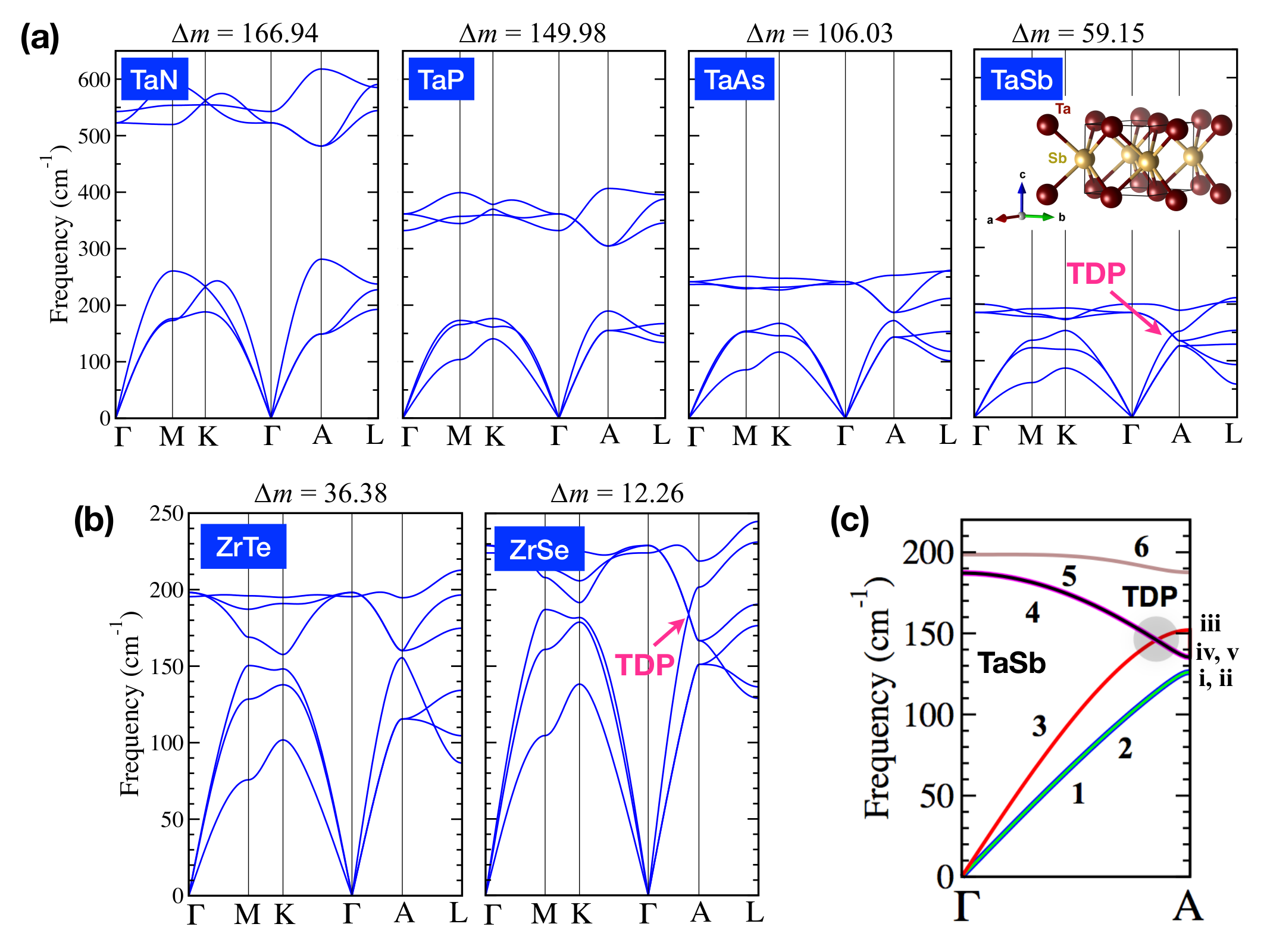
Figure 13: Phonon dispersion of (a) Ta$X$ ($X$ = N, P, As, Sb), and (b) Zr$Y$ ($Y$ = Se, Te) binaries calculated using the Density functional perturbation theory (DFPT) for supercell of size $2\times 2\times 2$. The mass difference $\Delta m$ is provided in $g/mol$ units. A prototype crystal structure of TaSb is given in the inset. The primitive unit cell contains one Ta and one $X$ (Sb) atoms at (2/3, 0.0, 2/3), and (0.0, 1/2, 0.0) sites, respectively. TDP is marked in the phonon spectrum of TaSb and ZrSe along $\Gamma$-A path. (c) An enlarged view of phonon dispersion in TaSb along $\Gamma$-A path. Colors and numbers depict distinct phonon modes. Arabic (Roman) numerals are used to mark phonon modes before (after) the band-inversion. Some data from Ref. [41] have been reused to produce this figure.

Figure 13(a) shows the calculated phonon spectra of Ta$X$ ($X$ = N, P, As, Sb) binaries having $\Delta m$ in decreasing order [41]. As the $X$ atom in Ta$X$ gets heavier, the frequency of optical phonons lowers, causing a systematic decrease in the frequency bandgap with decreasing $\Delta m$, and a phonon band-inversion takes place in TaSb along the $\Gamma$-A direction of Brillouin zone, where two degenerate optical phonon modes acquire lower frequency than a non-degenerate acoustic phonon mode. This phonon band-inversion results in a gapless triply degenerate point (TDP) in the phonon spectrum of TaSb at frequency $\sim$ 145 cm^-1 and at $q$ = (0, 0, 0.428). This point is marked in Figure 13(a). As shown in Fig. 13(b), a similar mass induced phonon band-inversion also occurs in Zr$Y$ ($Y$ = Se, Te) family. Zr$Y$ binaries are isostructural and isoelectronic to Ta$X$ [96]. In ZrTe, there exists a finite positive $\Delta_{g}$ due to the relatively large $\Delta m$. Whereas, the net frequency gap closes in ZrSe, which has relatively smaller $\Delta m$, and $\Delta_{g}$ becomes negative at the A-point due to the observed phonon band-inversion along $\Gamma$-A path.

An enlarged view of the phonon dispersion along the $\Gamma$-A direction of TaSb is shown in Fig. 13(c). In this figure, the degeneracy of phonon modes and formation of a TDP can be clearly observed. Another TDP is located in other direction in the Brillouin zone at the same $C_{3v}$-symmetric line. The two degenerate optical phonon modes participating in the phonon band-crossing at TDP correspond to the in-plane ($x-y$) optical vibrations of atoms, whereas the non-degenerate acoustic mode involved in the phonon band-crossing at TDP belong to the out-of-plane ($z$) acoustic vibration of atoms. The competition between in-plane and out-of-plane interatomic force constants, and $\Delta m$ is the primary reason of the phonon-band inversion in TaSb and ZrSe [41].

We note that the same methods [47, 121] that are used to compute the topological character of electronic band-crossings can also be employed to evaluate the topology of phonon band-crossings. However, it turns out that capturing the topology of phonon band-crossings is different from that of the electronic case. In case of non-interacting electronic systems, we analyze the symmetrized Hamiltonian of system for topological classification of the studied system. Topological classification of phononic systems can be build using the dynamical matrices $D({\bf q})$.

Similar to the case of triple-points in the electronic spectrum [21], gapless TDPs in the phonon spectrum are connected by a gapless nodal line in the phonon frequency space. This nodal line, shown in Fig. 14(d), is formed by the degenerate optical phonon modes near the TDP, and it is being protected by the $C_{3v}$ rotational symmetry of the crystal. Under the $C_{3v}$ symmetry, the $xx$ and $yy$ interatomic force constants transform just like the $p_{x}$ and $p_{y}$ orbitals in $C_{3v}$ group forming a 2D irreducible representation $E$, which enforces the degeneracy of optical phonon modes along $\Gamma$-A. Computation of Berry phase ($\phi_{B}$) using the Wilson loop approach along path $S^{1}$, as shown in Fig. 14(d), reveals $\phi_{B}=0$ for the gapless nodal line connecting two TDPs [41].

In order to reveal the topology of a TDP, one can split the two connected TDPs by breaking the $C_{3v}$ symmetry. This can be done by changing the $xx$ and $yy$ entries in the $D({\bf q})$, which is equivalent of tuning the interatomic force-constants (or equivalently, classical spring constants) between atoms along $x$ and $y$ directions [41]. This trick lifts up the degeneracy of the optical phonon modes, as shown in Fig. 14(b-c), and enables us to probe the topological nature of TDP. It is worth noting that the aforementioned trick does not destroy the gapless nodal line, rather it results in a gapless nodal loop formed by the inverted optical and acoustic phonon bands (see Fig. 14(e-f)). We can now define a path $S^{2}$ (and $S^{3}$) enclosing the gapless nodal loop, and compute the $\phi_{B}$ using the Wilson loop approach as demonstrated in Fig. 14(e-f). This calculation results in $\phi_{B}$ = $\pi$ for $S^{2}$ and $S^{3}$ paths, thus confirming the topological nature of TDP [41]. The mentioned technique is analogous to splitting two triple-point nodes in the electronic spectrum into four Weyl nodes by applying a Zeeman field [21].

The nontrivial topology of phonon band-crossings in bulk indicates the presence of nontrivial surface phonon states [41]. In fact, Li et al. predicted unusual phonon surface states (open gapless arcs) in TiS and HfTe compounds, which are triple-point metals hosting TDPs [96].

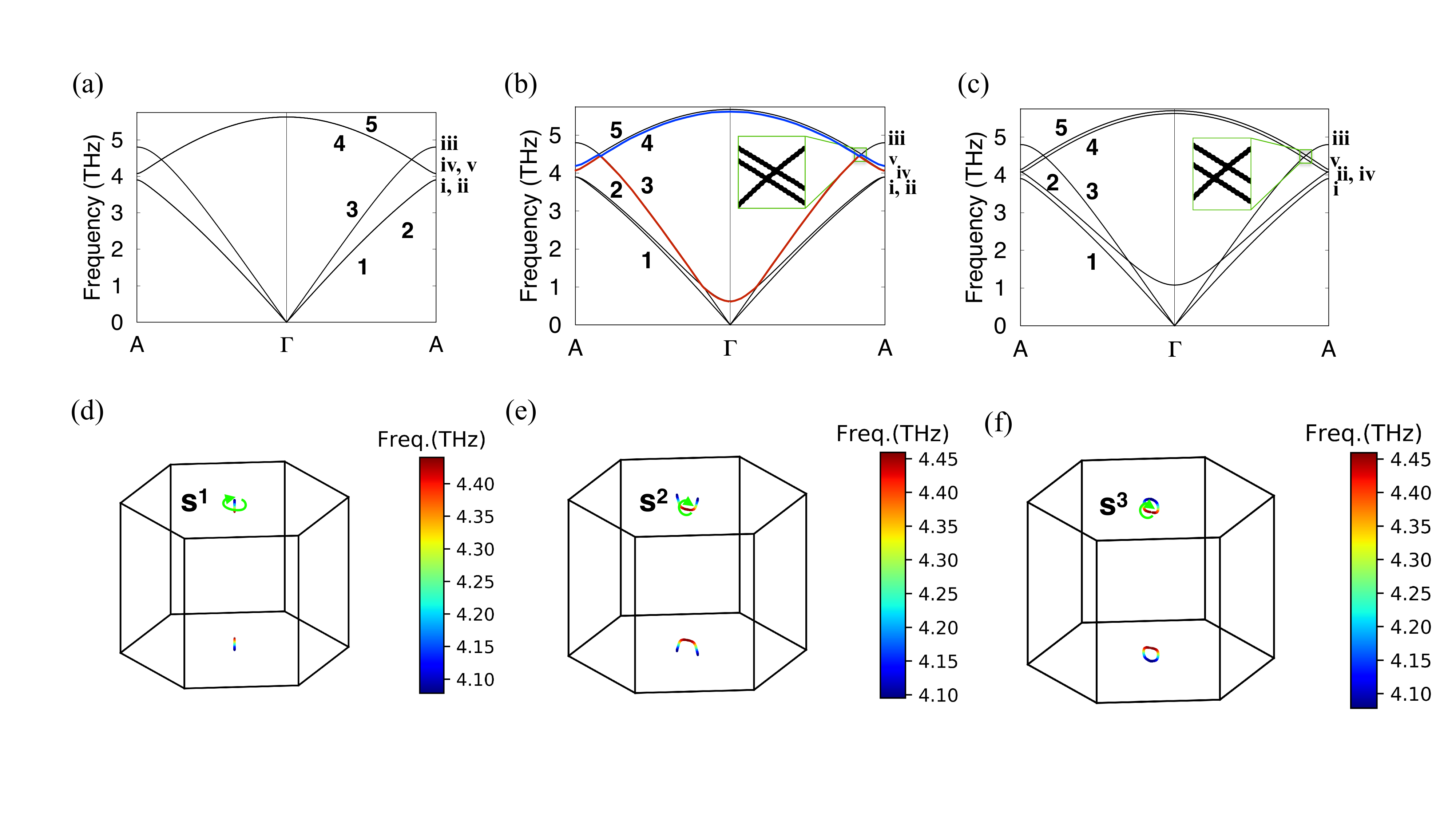
Figure 14: (a) The phonon spectrum of TaSb along the $C_{3v}$-symmetric line of the Brillouin zone: Doubly degenerate phonon bands (4,5) and (iv,v) can be seen. (b) The phonon spectrum of TaSb with the $xx$ and $yy$ force constants in the dynamical matrix made unequal for Ta. The degeneracy of (4,5) and (iv, v) is lifted. (c) The phonon spectrum of TaSb with the $xx$ and $yy$ force constants in the dynamical matrix made unequal for Sb. The degeneracy of (4,5) and (iv, v) is lifted. (d) The non-topological open nodal line formed in the BZ by bands iv and v of panel (a). The loop $S^{1}$ encircles this line, but $\phi_{B}(S^{1})=0$. (e) The closed nodal loop formed by bands iv and v in the BZ for the case of panel (b) away from the $\Gamma$-A line. The contour $S^{2}$ links with this loop and $\phi_{B}(S^{2})=\pi$. (f) The closed nodal loop formed by bands iv and v in the BZ for the case of panel (c). For a contour $S^{3}$ linked with this loop $\phi_{B}(S^{3})=\pi$. Figure adopted from Ref. [41] with permission.

6 Thermoelectricity in triple-point metals

Since the nontrivial topology of electronic bands is often manifested in the electronic transport measurements, the phonon topology could have observable signatures in the lattice thermal transport measurements. It has been reported that topologically protected nontrivial phonon band-crossings introduce robust phonon-phonon scattering centers that enormously suppress the lattice thermal conductivity ($\kappa_{ph}$) in triple-point metals hosting TDPs [41]. In Figure 15(a), we compare the $\kappa_{ph}$ of two isostructural and isoelectronic triple-point metals– TaN and TaSb, where the later hosts TDPs whereas the former does not. We notice that the overall $\kappa_{ph}$ in TaSb is almost three orders in magnitude smaller than that of in TaN. Such a large reduction in $\kappa_{ph}$ causes a direct benefit towards the improved thermoelectric performance of triple-point metals hosting TDPs [41].

The thermoelectric figure of merit, $ZT$ = $\frac{S^{2}\sigma}{\kappa_{el}+\kappa_{ph}}T$, is the key indicator of the thermoelectric performance of any material. To achieve large $ZT$, one requires large thermopower or Seebeck coefficient ($S$), high electrical conductivity ($\sigma$), low electronic thermal conductivity ($\kappa_{el}$), and low lattice thermal conductivity ($\kappa_{ph}$) at a given temperature (T). Unfortunately, $\sigma$ and $\kappa_{el}$ are intrinsically coupled following the Wiedemann-Franz law, i.e. $\kappa_{el}=L_{0}T\sigma$, where $L_{0}$ is the Lorenz number [122]. Therefore, an optimal balance is required between $\sigma$ and $\kappa_{el}$. Another key factor is the thermopower or Seebeck coefficient ($S$) which is primarily governed by the electronic electronic density of states near the Fermi-level. Generally, narrow bandgap semiconductors (with small $\kappa_{el}+\kappa_{ph}$) exhibit the best thermoelectric performance ($ZT$ $\sim$ 2-3) when slightly doped by $n-$ or $p-$type charge carriers [122, 123, 124, 125, 126, 127]. Whereas, metals are known to be poor thermoelectrics due to their large $\sigma$ and large $\kappa_{el}$ (because of no energy bandgap). Moreover, $\kappa_{ph}$ is also considerably large in most of the metals, thus, overall $ZT$ is quite low in metals ranging from $0.0001$ – $0.001$ [128, 129, 130].

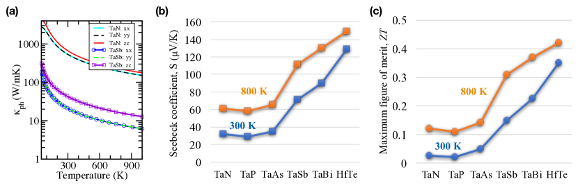
Figure 15: (a) Comparison of the calculated lattice thermal conductivity ($\kappa_{ph}$) versus temperature data for TaN and TaSb binaries. Vertical axis is in logarithmic scale. (b) The maximum estimated thermopower or Seebeck coefficient, and (c) maximum estimated thermoelectric figure of merit computed at 300 K and 800 K for electronic doping case. Data from Ref. [41] is reused to produce this figure.

The triple-point metals hosting TDPs seem to be special metals having considerably large and sizable $ZT$. The maximum estimated $ZT$ in triple-point metals hosting TDPs ranges from $\sim$0.15 (at room temperature) to $\sim$0.4 (at 800 K) [41]. Remarkably, in HfTe (which is a triple-point metal hosting TDPs) the maximum estimated $ZT$ ranges from 0.35 (at 300 K) to 0.42 (at 800 K) for electron doping (see Fig. 15(b-c)). Evidently, the thermoelectric performance of triple-point metals hosting TDPs is 2–3 orders in magnitude larger than that of the trivial metals [41].

Two key factors combine to enhance the net $ZT$ in triple-point metals. First, the presence of TDP, which gives rise to reduced $\kappa_{ph}$. Second, the nontrivial electronic band-crossings near the Fermi-level, i.e. the presence of gapless Weyl/Triple-points fermions yields large $\sigma$ (unfortunately, $\kappa_{el}$ is also large) as well as enhanced thermopower $S$. Notably, $\sigma$ lies in the same order of magnitude ($\sigma/\tau\sim 10^{20}\,1/{$\mathrm{\SIUnitSymbolOhm}$}ms$ at low-doping concentrations, $\tau$ being the electron-phonon relaxation time) for all the yet studied triple-point metals [41]. Gapless points near the Fermi-level give rise to sharp enhancement in the electronic density of states near the Fermi-level, which increases $S$ according to the Mahan-Sofo theory [131]. Thus, triple-point metals with TDPs inherit high $S$, high $\sigma$, and low $\kappa_{ph}$, which consequently yields relatively better thermoelectric performance in such metals. Figures 15(b-c) compare the thermopower ($S$) and thermoelectric performance ($ZT$) of selected triple-point metals with and without TDPs in their phonon spectra. For more technical details regarding the calculation of vibrational and thermoelectric properties, we recommend the reader to Ref. [41].

7 Concluding Remarks

We have overviewed the theoretical and experimental progress in the field of triple-point fermions protected by symmorphic symmetries. While the topological classification and basic band structure of triple-points are now well understood, open challenges lie ahead in investigating the transport and optical properties. In particular low temperature applications could arise due to the presence of direction dependent magnetotransport.

Experimentalists are always in need of more accessible material candidates to confirm the manifold theoretical predictions. Recent experimental progress has been made for MoP [35, 36], where the existence of triple-points has been directly confirmed by ARPES, and WC [33, 34], of which the fermi arcs and magnetotransport of triple-points have been investigated. To improve on this studies materials with good growth characteristics and well separated triple-points close to the Fermi level are desired. The recently predicted half-Heusler materials seem to have very favorable properties in this respect [44].

Lastly, we have surveyed the topology of phonons in condensed matter systems, particularly in triple-point metals, and also discussed the numerical techniques required to evaluate the nontrivial topological nature of the triple-point nodes present in the phonon spectrum. The presence of topological phonon band-crossings usually introduce phonon-phonon scattering centers yielding low lattice thermal conductivity (phonon glass), whereas presence of gapless topological nodes near the Fermi-level yield good electrical conductivity and thermopower (electron crystal). These two factors (electron crystal + phonon glass) combine to improve the thermoelectric performance of certain triple-point metals that host TDPs in their phonon spectra. Although the thermoelectric performance of triple-point metals is not comparable to that of the best known thermoelectrics (it is obviously expected given the metallicity), triple-point metals with topological phonon band-crossings rank much better when compared to the thermoelectricity of ordinary metals.

To conclude, the discovery and description of triple-point metals will allow for further progress in understanding topological phenomena in solids and identification of topological materials with potential applications in technology. The triple-point fermion has been accepted as an integral part of the family of topological (semi-) metals.

References

- [1] Weng H, Fang C, Fang Z, Bernevig B A and Dai X 2015 Phys. Rev. X 5(1) 011029
- [2] Huang S M, Xu S Y, Belopolski I, Lee C C, Chang G, Wang B, Alidoust N, Bian G, Neupane M, Zhang C, Jia S, Bansil A, Lin H and Hasan M Z 2015 Nat Commun 6
- [3] Xu S Y, Belopolski I, Alidoust N, Neupane M, Bian G, Zhang C, Sankar R, Chang G, Yuan Z, Lee C C, Huang S M, Zheng H, Ma J, Sanchez D S, Wang B, Bansil A, Chou F, Shibayev P P, Lin H, Jia S and Hasan M Z 2015 Science 349 613–617
- [4] Lv B Q, Weng H M, Fu B B, Wang X P, Miao H, Ma J, Richard P, Huang X C, Zhao L X, Chen G F, Fang Z, Dai X, Qian T and Ding H 2015 Phys. Rev. X 5(3) 031013
- [5] Lv B Q, Xu N, Weng H M, Ma J Z, Richard P, Huang X C, Zhao L X, Chen G F, Matt C E, Bisti F, Strocov V N, Mesot J, Fang Z, Dai X, Qian T, Shi M and Ding H 2015 Nat Phys 11 724–727
- [6] Wan X, Turner A M, Vishwanath A and Savrasov S Y 2011 Phys. Rev. B 83(20) 205101
- [7] Wang Z, Sun Y, Chen X Q, Franchini C, Xu G, Weng H, Dai X and Fang Z 2012 Phys. Rev. B 85(19) 195320
- [8] Wang Z, Weng H, Wu Q, Dai X and Fang Z 2013 Phys. Rev. B 88(12) 125427
- [9] Liu Z K, Jiang J, Zhou B, Wang Z J, Zhang Y, Weng H M, Prabhakaran D, Mo S K, Peng H, Dudin P, Kim T, Hoesch M, Fang Z, Dai X, Shen Z X, Feng D L, Hussain Z and Chen Y L 2014 Nat Mater 13 677–681
- [10] Xu S Y, Liu C, Kushwaha S K, Sankar R, Krizan J W, Belopolski I, Neupane M, Bian G, Alidoust N, Chang T R, Jeng H T, Huang C Y, Tsai W F, Lin H, Shibayev P P, Chou F C, Cava R J and Hasan M Z 2015 Science 347 294–298
- [11] Soluyanov A A, Gresch D, Wang Z, Wu Q, Troyer M, Dai X and Bernevig B A 2015 Nature 527(7579) 495
- [12] Wang Z, Alexandradinata A, Cava R J and Bernevig B A 2016 Nature 532 189–194
- [13] Kim Y, Wieder B J, Kane C L and Rappe A M 2015 Phys. Rev. Lett. 115(3) 036806
- [14] Bzdušek T, Wu Q, Rüegg A, Sigrist M and Soluyanov A A 2016 Nature 538 75–78
- [15] Kruthoff J, de Boer J, van Wezel J, Kane C L and Slager R J 2017 Phys. Rev. X 7(4) 041069
- [16] Wieder B J, Kim Y, Rappe A M and Kane C L 2016 Phys. Rev. Lett. 116(18) 186402
- [17] Bradlyn B, Cano J, Wang Z, Vergniory M G, Felser C, Cava R J and Bernevig B A 2016 Science 353
- [18] Burkov A A, Hook M D and Balents L 2011 Phys. Rev. B 84(23) 235126
- [19] Parameswaran S A, Turner A M, Arovas D P and Vishwanath A 2013 Nat Phys 9 299–303
- [20] Winkler G W, Wu Q, Troyer M, Krogstrup P and Soluyanov A A 2016 Phys. Rev. Lett. 117(7) 076403
- [21] Zhu Z, Winkler G W, Wu Q, Li J and Soluyanov A A 2016 Phys. Rev. X 6(3) 031003
- [22] Weng H, Fang C, Fang Z and Dai X 2016 Phys. Rev. B 93(24) 241202
- [23] Koster G 1963 Properties of the thirty-two point groups Massachusetts institute of technology press research monograph (M.I.T. Press)
- [24] Aroyo M I, Orobengoa D, de la Flor G, Tasci E S, Perez-Mato J M and Wondratschek H 2014 Acta Crystallographica Section A 70 126–137
- [25] Bradley C and Cracknell A 2010 The Mathematical Theory of Symmetry in Solids: Representation Theory for Point Groups and Space Groups EBSCO ebook academic collection (OUP Oxford) ISBN 9780199582587
- [26] Alexandradinata A, Dai X and Bernevig B A 2014 Phys. Rev. B 89(15) 155114
- [27] Chan Y H, Chiu C K, Chou M Y and Schnyder A P 2016 Phys. Rev. B 93(20) 205132
- [28] Weng H, Liang Y, Xu Q, Yu R, Fang Z, Dai X and Kawazoe Y 2015 Phys. Rev. B 92(4) 045108
- [29] Volovik G 2009 The Universe in a Helium Droplet International Series of Monographs on Physics (OUP Oxford) ISBN 9780199564842
- [30] Mikitik G P and Sharlai Y V 2008 Low Temperature Physics 34 794–800
- [31] Heikkilä T T and Volovik G E 2015 New Journal of Physics 17 093019
- [32] Hyart T and Heikkilä T T 2016 Phys. Rev. B 93(23) 235147
- [33] He J B, Chen D, Zhu W L, Zhang S, Zhao L X, Ren Z A and Chen G F 2017 Phys. Rev. B 95(19) 195165
- [34] Ma J Z, He J B, Xu Y F, Lv B Q, Chen D, Zhu W L, Zhang S, Kong L Y, Gao X, Rong L Y, Huang Y B, Richard P, Xi C Y, Shao Y, Wang Y L, Gao H J, Dai X, Fang C, Weng H M, Chen G F, Qian T and Ding H 2017 arXiv:1706.02664
- [35] Lv B Q, Feng Z L, Xu Q N, Gao X, Ma J Z, Kong L Y, Richard P, Huang Y B, Strocov V N, Fang C, Weng H M, Shi Y G, Qian T and Ding H 2017 Nature 546 627–631
- [36] Shekhar C, Sun Y, Kumar N, Nicklas M, Manna K, Suess V, Young O, Leermakers I, Foerster T, Schmidt M, Muechler L, Werner P, Schnelle W, Zeitler U, Yan B, Parkin S S P and Felser C 2017 arXiv:1703.03736
- [37] Suchalkin S, Belenky G, Ermolaev M, Moon S, Jiang Y, Graf D, Smirnov D, Laikhtman B, Shterengas L, Kipshidze G, Svensson S P and Sarney W L 2017 arXiv:1705.02509
- [38] Sun J P, Zhang D and Chang K 2017 Chinese Physics Letters 34 027102
- [39] Weng H, Fang C, Fang Z and Dai X 2016 Phys. Rev. B 94(16) 165201
- [40] Sun J P, Zhang D and Chang K 2017 arXiv:1705.05061
- [41] Singh S, Wu Q, Yue C, Romero A H and Soluyanov A A 2018 Phys. Rev. Materials 2(11) 114204
- [42] Zaheer S, Young S M, Cellucci D, Teo J C Y, Kane C L, Mele E J and Rappe A M 2013 Phys. Rev. B 87(4) 045202
- [43] Sheng X L, Yu Z M, Yu R, Weng H and Yang S A 2017 arXiv:1703.09040
- [44] Yang H, Yu J, Parkin S S P, Felser C, Liu C X and Yan B 2017 arXiv:1706.00200
- [45] Teo J C Y, Fu L and Kane C L 2008 Phys. Rev. B 78(4) 045426
- [46] Heyd J, Scuseria G E and Ernzerhof M 2003 The Journal of Chemical Physics 118 8207–8215
- [47] Wu Q, Zhang S, Song H F, Troyer M and Soluyanov A A 2018 Computer Physics Communications 224 405 – 416
- [48] Yu J, Yan B and Liu C X 2017 arXiv:1704.01138
- [49] Liu C, Lee Y, Kondo T, Mun E D, Caudle M, Harmon B N, Bud’ko S L, Canfield P C and Kaminski A 2011 Phys. Rev. B 83(20) 205133
- [50] Liu Z K, Yang L X, Wu S C, Shekhar C, Jiang J, Yang H F, Zhang Y, Mo S K, Hussain Z, Yan B, Felser C and Chen Y L 2016 Nature Communications 7 12924
- [51] Stringfellow G B and Chen G S 1991 Journal of Vacuum Science & Technology B 9 2182–2188
- [52] Cripps S, Hosea T, Krier A, Smirnov V, Batty P, Zhuang Q, Lin H, Liu P and Tsai G 2008 Thin Solid Films 516 8049–8058
- [53] Svensson S P, Sarney W L, Hier H, Lin Y, Wang D, Donetsky D, Shterengas L, Kipshidze G and Belenky G 2012 Phys. Rev. B 86(24) 245205
- [54] Suchalkin S, Ludwig J, Belenky G, Laikhtman B, Kipshidze G, Lin Y, Shterengas L, Smirnov D, Luryi S, Sarney W and Svensson S P 2016 Journal of Physics D: Applied Physics 49 105101
- [55] Jen H R, Ma K Y and Stringfellow G B 1989 Applied Physics Letters 54 1154–1156
- [56] Kurtz S R, Dawson L R, Biefeld R M, Follstaedt D M and Doyle B L 1992 Phys. Rev. B 46(3) 1909–1912
- [57] Wei S and Zunger A 1991 Applied Physics Letters 58 2684–2686
- [58] Belenky G, Lin Y, Shterengas L, Donetsky D, Kipshidze G and Suchalkin S 2015 Electronics Letters 51 1521–1522
- [59] Ivanov D A 2001 Phys. Rev. Lett. 86(2) 268–271
- [60] Read N and Green D 2000 Phys. Rev. B 61(15) 10267–10297
- [61] Kitaev A Y 2001 Physics-Uspekhi 44 131
- [62] Kitaev A 2003 Annals of Physics 303 2 – 30
- [63] Nayak C, Simon S H, Stern A, Freedman M and Das Sarma S 2008 Rev. Mod. Phys. 80(3) 1083–1159
- [64] Lutchyn R M, Sau J D and Das Sarma S 2010 Phys. Rev. Lett. 105(7) 077001
- [65] Oreg Y, Refael G and von Oppen F 2010 Phys. Rev. Lett. 105(17) 177002
- [66] Das A, Ronen Y, Most Y, Oreg Y, Heiblum M and Shtrikman H 2012 Nat Phys 8 887–895
- [67] Deng M T, Yu C L, Huang G Y, Larsson M, Caroff P and Xu H Q 2012 Nano Letters 12 6414–6419
- [68] Mourik V, Zuo K, Frolov S M, Plissard S R, Bakkers E P A M and Kouwenhoven L P 2012 Science 336 1003–1007
- [69] Albrecht S M, Higginbotham A P, Madsen M, Kuemmeth F, Jespersen T S, Nygård J, Krogstrup P and Marcus C M 2016 Nature 531 206–209
- [70] Zhang H, Gül Ö, Conesa-Boj S, Zuo K, Mourik V, de Vries F K, van Veen J, van Woerkom D J, Nowak M P, Wimmer M, Car D, Plissard S, Bakkers E P A M, Quintero-Pérez M, Goswami S, Watanabe K, Taniguchi T and Kouwenhoven L P 2016 arXiv:1603.04069
- [71] Yu R, Qi X L, Bernevig A, Fang Z and Dai X 2011 Phys. Rev. B 84(7) 075119
- [72] Sgiarovello C, Peressi M and Resta R 2001 Phys. Rev. B 64(11) 115202
- [73] Fu L and Kane C L 2006 Phys. Rev. B 74(19) 195312
- [74] Soluyanov A A and Vanderbilt D 2011 Phys. Rev. B 83(23) 235401
- [75] Gresch D, Autès G, Yazyev O V, Troyer M, Vanderbilt D, Bernevig B A and Soluyanov A A 2017 Phys. Rev. B 95(7) 075146
- [76] Fang C, Gilbert M J and Bernevig B A 2012 Phys. Rev. B 86(11) 115112
- [77] Soluyanov A A and Vanderbilt D 2012 Phys. Rev. B 85(11) 115415
- [78] Ezawa M 2017 Phys. Rev. B 95(20) 205201
- [79] Sengupta P, Ryu H, Lee S and Tan Y 2014 arXiv:1409.4376
- [80] Sancho M P L, Sancho J M L and Rubio J 1984 Journal of Physics F: Metal Physics 14 1205
- [81] Sancho M P L, Sancho J M L and Rubio J 1985 Journal of Physics F: Metal Physics 15 851
- [82] Adler S L 1969 Phys. Rev. 177(5) 2426–2438
- [83] Bell J S and Jackiw R 1969 Il Nuovo Cimento A (1971-1996) 60 47–61
- [84] Nielsen H and Ninomiya M 1983 Physics Letters B 130 389 – 396
- [85] Hosur P and Qi X 2013 Comptes Rendus Physique 14 857 – 870
- [86] Son D T and Spivak B Z 2013 Phys. Rev. B 88(10) 104412
- [87] Jeon S, Zhou B B, Gyenis A, Feldman B E, Kimchi I, Potter A C, Gibson Q D, Cava R J, Vishwanath A and Yazdani A 2014 Nat Mater 13 851–856
- [88] Burkov A A and Kim Y B 2016 Phys. Rev. Lett. 117(13) 136602
- [89] Kane C L and Lubensky T C 2014 Nat Phys 10 39–45
- [90] Stenull O, Kane C L and Lubensky T C 2016 Phys. Rev. Lett. 117(6) 068001
- [91] Süsstrunk R and Huber S D 2015 Science 349 47–50
- [92] Süsstrunk R and Huber S D 2016 Proceedings of the National Academy of Sciences 113 E4767–E4775
- [93] Huber S D 2016 Nat Phys 12 621–623
- [94] Zhang T, Song Z, Alexandradinata A, Weng H, Fang C, Lu L and Fang Z 2018 Phys. Rev. Lett. 120(1) 016401
- [95] Esmann M, Lamberti F R, Senellart P, Favero I, Krebs O, Lanco L, Gomez Carbonell C, Lemaître A and Lanzillotti-Kimura N D 2018 Phys. Rev. B 97(15) 155422
- [96] Li J, Xie Q, Ullah S, Li R, Ma H, Li D, Li Y and Chen X Q 2018 Phys. Rev. B 97(5) 054305
- [97] Xie Q, Li J, Liu M, Wang L, Li D, Li Y and Chen X Q 2018 arXiv:1801.04048
- [98] Miao H, Zhang T T, Wang L, Meyers D, Said A H, Wang Y L, Shi Y G, Weng H M, Fang Z and Dean M P M 2018 Phys. Rev. Lett. 121(3) 035302
- [99] Zhang L, Ren J, Wang J S and Li B 2010 Phys. Rev. Lett. 105(22) 225901
- [100] Zhang L and Niu Q 2015 Phys. Rev. Lett. 115(11) 115502
- [101] Wang P, Lu L and Bertoldi K 2015 Phys. Rev. Lett. 115(10) 104302
- [102] Lu J, Qiu C, Ye L, Fan X, Ke M, Zhang F and Liu Z 2016 Nature Physics 13 369
- [103] Fleury R, Khanikaev A B and Alù A 2016 Nature Communications 7 11744
- [104] Peng Y G, Qin C Z, Zhao D G, Shen Y X, Xu X Y, Bao M, Jia H and Zhu X F 2016 Nature Communications 7 13368
- [105] Liu Y, Lian C S, Li Y, Xu Y and Duan W 2017 Phys. Rev. Lett. 119(25) 255901
- [106] Liu Y, Xu Y, Zhang S C and Duan W 2017 Phys. Rev. B 96(6) 064106
- [107] Liu Y, Xu Y and Duan W 2017 National Science Review 5 314–316
- [108] Jin Y, Wang R and Xu H 2018 Nano Letters 18 7755–7760
- [109] Zhang X, Xiao M, Cheng Y, Lu M H and Christensen J 2018 Communications Physics 1 97
- [110] Raghu S and Haldane F D M 2008 Phys. Rev. A 78(3) 033834
- [111] Mei J, Wu Y, Chan C T and Zhang Z Q 2012 Phys. Rev. B 86(3) 035141
- [112] Sun K, Liu W V, Hemmerich A and Das Sarma S 2012 Nat Phys 8 67–70
- [113] Khanikaev A B, Hossein Mousavi S, Tse W K, Kargarian M, MacDonald A H and Shvets G 2013 Nat Mater 12 233–239
- [114] Lu L, Fu L, Joannopoulos J D and Soljacic M 2013 Nat Photon 7 294–299
- [115] Rechtsman M C, Plotnik Y, Zeuner J M, Song D, Chen Z, Szameit A and Segev M 2013 Phys. Rev. Lett. 111(10) 103901
- [116] Lu L, Joannopoulos J D and Soljacic M 2014 Nat Photon 8 821–829
- [117] He W Y and Chan C T 2015 Scientific reports 5 8186
- [118] Liu S and Hou Q 2017 Journal of Physics B: Atomic, Molecular and Optical Physics 50 245001
- [119] Fulga I C, Fallani L and Burrello M 2018 Phys. Rev. B 97(12) 121402
- [120] Prodan E and Prodan C 2009 Phys. Rev. Lett. 103(24) 248101
- [121] Gresch D, Autès G, Yazyev O V, Troyer M, Vanderbilt D, Bernevig B A and Soluyanov A A 2017 Phys. Rev. B 95(7) 075146
- [122] Snyder G J and Toberer E S 2008 Nature Materials 7 105
- [123] Rowe D M 2005 Thermoelectrics handbook: macro to nano (CRC press)
- [124] Zhao L D, Lo S H, Zhang Y, Sun H, Tan G, Uher C, Wolverton C, Dravid V P and Kanatzidis M G 2014 Nature 508 373
- [125] Duong A T, Nguyen V Q, Duvjir G, Duong V T, Kwon S, Song J Y, Lee J K, Lee J E, Park S, Min T, Lee J, Kim J and Cho S 2016 Nature Communications 7 13713
- [126] Zhao L D, Tan G, Hao S, He J, Pei Y, Chi H, Wang H, Gong S, Xu H, Dravid V P, Uher C, Snyder G J, Wolverton C and Kanatzidis M G 2016 Science 351 141–144
- [127] Singh S, Ibarra-Hernandez W, Valencia-Jaime I, Avendano-Franco G and Romero A H 2016 Phys. Chem. Chem. Phys. 18(43) 29771–29785
- [128] Terasaki I, Sasago Y and Uchinokura K 1997 Phys. Rev. B 56(20) R12685–R12687
- [129] Takahata K, Iguchi Y, Tanaka D, Itoh T and Terasaki I 2000 Phys. Rev. B 61(19) 12551–12555
- [130] Okuda T, Nakanishi K, Miyasaka S and Tokura Y 2001 Phys. Rev. B 63(11) 113104
- [131] Mahan G D and Sofo J O 1996 Proceedings of the National Academy of Sciences 93 7436–7439