Nonlinear Craig Interpolant Generation

Abstract

Interpolation-based techniques have become popular in recent years because of their inherently modular and local reasoning, which can scale up existing formal verification techniques like theorem proving, model-checking, abstraction interpretation, and so on, while the scalability is the bottleneck of these techniques. Craig interpolant generation plays a central role in interpolation-based techniques, and therefore has drawn increasing attention. In the literature, there are various works done on how to automatically synthesize interpolants for decidable fragments of first-order logic, linear arithmetic, array logic, equality logic with uninterpreted functions (EUF), etc., and their combinations. But Craig interpolant generation for non-linear theory and its combination with the aforementioned theories are still in infancy, although some attempts have been done. In this paper, we first prove that a polynomial interpolant of the form $h(\mathbf{x})>0$ exists for two mutually contradictory polynomial formulas $\phi(\mathbf{x},\mathbf{y})$ and $\psi(\mathbf{x},\mathbf{z})$, with the form $f_{1}\geq 0\wedge\cdots\wedge f_{n}\geq 0$, where $f_{i}$ are polynomials in $\mathbf{x},\mathbf{y}$ or $\mathbf{x},\mathbf{z}$, and the quadratic module generated by $f_{i}$ is Archimedean. Then, we show that synthesizing such interpolant can be reduced to solving a semi-definite programming problem (${\rm SDP}$). In addition, we propose a verification approach to assure the validity of the synthesized interpolant and consequently avoid the unsoundness caused by numerical error in ${\rm SDP}$ solving. Then, we discuss how to generalize our approach to general semi-algebraic formulas. Finally, as an applicaiton of our approach, we demonstrate how to apply it to invariant generation in program verification.

raig interpolant, Archimedean condition, semi-definite programming, program verification, sum of squares

1 Introduction

Interpolation-based techniques have become popular in recent years because of their inherently modular and local reasoning, which can scale up existing formal verification techniques like theorem proving, model-checking, abstract interpretation, and so on, while the scalability is the bottleneck of these techniques. The study of interpolation was pioneered by Kraj${\rm\acute{i}\breve{c}}$ek krajicek97 and Pudlák pudlak97 in connection with theorem proving, by McMillan in connection with model-checking mcmillan03 , by Graf and Saïdi GS97 , Henzinger et al. HJMM04 and McMillan mcmillan05 in connection with abstraction like CEGAR, by Wang et al. wang11 in connection with machine-learning based program verification.

Craig interpolant generation plays a central role in interpolation-based techniques, and therefore has drawn increasing attention. In the literature, there are various efficient algorithms proposed for automatically synthesizing interpolants for various theories, e.g., decidable fragments of first-order logic, linear arithmetic, array logic, equality logic with uninterpreted functions (EUF), etc., and their combinations, and their use in verification mcmillan05 ; HJMM04 ; YM05 ; KMZ06 ; RS10 ; KV09 ; CGS08 ; mcmillan08 . In mcmillan05 , McMillan presented a method for deriving Craig interpolants from proofs in the quantifier-free theory of linear inequality and uninterpreted function symbols, and based on which an interpolating theorem prover was provided. In HJMM04 , Henzinger et al. proposed a method to synthesize Craig interpolants for a theory with arithmetic and pointer expressions, as well as call-by-value functions. In YM05 , Yorsh and Musuvathi presented a combination method to generate Craig interpolants for a class of first-order theories. In KMZ06 , Kapur et al. presented different efficient procedures to construct interpolants for the theories of arrays, sets and multisets using the reduction approach. Rybalchenko and Sofronie-Stokkermans RS10 proposed an approach to reducing the synthesis of Craig interpolants of the combined theory of linear arithmetic and uninterpreted function symbols to constraint solving. In addition, D’Silva et al. SPWK10 investigated strengths of various interpolants.

However, interpolant generation for non-linear theory and its combination with the aforementioned theories is still in infancy, although nonlinear polynomials inequalities are quite common in software involving number theoretic functions as well as hybrid systems ZZKL12 ; Zhan17 . In DXZ13 , Dai et al. had a first try and gave an algorithm for generating interpolants for conjunctions of mutually contradictory nonlinear polynomial inequalities based on the existence of a witness guaranteed by Stengle’s Positivstellensatz Stengle , which is computable using semi-definite programming (${\rm SDP}$). Their algorithm is incomplete in general but if all variables are bounded (called Archimedean condition), then their algorithm is complete. A major limitation of their work is that two mutually contradictory formulas $\phi$ and $\psi$ must have the same set of variables. In GDX16 , Gan et al. proposed an algorithm to generate interpolants for quadratic polynomial inequalities. The basic idea is based on the insight that for analyzing the solution space of concave quadratic polynomial inequalities, it suffices to linearize them. A generalization of Motzkin’s transposition theorem is proved to be applicable for concave quadratic polynomial inequalities. Using this, they proved the existence of an interpolant for two mutually contradictory conjunctions $\phi(\mathbf{x},\mathbf{y}),\psi(\mathbf{x},\mathbf{z})$ of concave quadratic polynomial inequalities and proposed an ${\rm SDP}$-based algorithm to compute it. Also in GDX16 , they developed a combination algorithm for generating interpolants for the combination of quantifier-free theory of concave quadratic polynomial inequalities and EUF based on the hierarchical calculus framework proposed in SSLMCS2008 and used in RS10 . Obviously, quadratic concave polynomial inequalities is a very restrictive class of polynomial formulas, although most of existing abstract domains fall within it as argued in GDX16 . Meanwhile, in GZ16 , Gao and Zufferey presented an approach to extract interpolants for non-linear formulas possibly containing transcendental functions and differential equations from proofs of unsatisfiability generated by $\delta$-decision procedure Gao14 that are based on interval constraint propagation (ICP) BG06 . Similar idea was also reported in KB11 . They transform proof traces from $\delta$-complete decision procedures into interpolants that consist of Boolean combinations of linear constraints. Thus, their approach can only find the interpolants between two formulas whenever their conjunction is not $\delta$-satisfiable.

Example 1

Let

$$\phi = -2xy^{2}+x^{2}-3xz-y^{2}-yz+z^{2}-1\geq 0\wedge 100-x^{2}-y^{2}\geq 0\wedge$$

$$x^{2}z^{2}+y^{2}z^{2}-x^{2}-y^{2}+\frac{1}{6}(x^{4}+2x^{2}y^{2}+y^{4})-\frac{1}{120}(x^{6}+y^{6})-4\leq 0;$$

$$\psi = 4(x-y)^{4}+(x+y)^{2}+w^{2}-133.097\leq 0\wedge 100(x+y)^{2}-w^{2}(x-y)^{4}-3000\geq 0.$$

It can be checked that $\phi\wedge\psi\models\bot$.

Obviously, synthesizing interpolants for $\phi$ and $\psi$ in this example is beyond the ability of the above approaches reported in DXZ13 ; GDX16 . Using the method in GZ16 implemented in dReal3 it would return “SAT” with $\delta=0.001$, i.e., $\phi\wedge\psi$ is $\delta$-satisfiable, and hence it cannot synthesize any interpolant using Gao14 ’s approach with any precision greater than $0.001$. While, using our method, an interpolant $h>0$ with degree $10$ can be found as shown in Fig LABEL:fig-twist, where,

$$h= 85.868928829-3.48171895438*x-4.05055570642*y+69.5179717355*y^{2}-$$

$$1.975586161*x*y^{2}+73.7505185252*x^{2}+79.7889009541*x^{4}+$$

$$39.4019812625*x^{2}*y^{2}+59.0193160126*y^{4}+5.81006679403*x^{6}-$$

$$2.92654531095*y^{6}+43.1570807435*x*y+25.0366942193*x*y^{3}+$$

$$34.8268489109*x^{3}*y+3.86714864443*x^{3}+4.04378820386*x^{2}*y-$$

$$5.94528747172*y^{3}+8.72599707958*x^{5}+2.97413012798*x^{4}*y-$$

$$6.09661882807*x^{3}*y^{2}-6.92712190458*x^{2}*y^{3}-9.98542713025*x*y^{4}-$$

$$13.6495929388*y^{5}-28.5122945936*x^{5}*y-7.3306401143*x^{4}*y^{2}-$$

$$12.8405648769*x^{3}*y^{3}-2.4656615978*x^{2}*y^{4}-25.914058476*x*y^{5}+$$

$$0.574487452756*x^{7}-2.04161159811*x^{6}*y-2.1652665291*x^{5}*y^{2}+$$

$$0.441933622851*x^{4}*y^{3}-3.31339953201*x^{3}*y^{4}-1.18860782739*x^{2}*y^{5}-$$

$$1.59589948759*x*y^{6}-0.207834237584*y^{7}-0.39416212619*x^{8}-$$

$$2.61990676298*x^{7}*y+10.5074625167*x^{6}*y^{2}-11.2424047363*x^{5}*y^{3}+$$

$$4.40746440558*x^{4}*y^{4}-8.71563327623*x^{3}*y^{5}+12.7151449616*x^{2}*y^{6}-$$

$$7.65894409136*x*y^{7}+0.997807267855*y^{8}+0.360026919214*x^{9}-$$

$$1.60158863204*x^{8}*y+1.72767640966*x^{7}*y^{2}+1.39706253748*x^{6}*y^{3}-$$

$$3.00346730309*x^{5}*y^{4}+0.232691322651*x^{4}*y^{5}-1.70644550812*x^{3}*y^{6}+$$

$$5.74945017152*x^{2}*y^{7}-4.80737336486*x*y^{8}+1.1814541304*y^{9}+$$

$$0.387479209367*x^{10}-2.45667500053*x^{9}*y+7.28054219791*x^{8}*y^{2}-$$

$$12.6714503175*x^{7}*y^{3}+14.875324384*x^{6}*y^{4}-14.7134968452*x^{5}*y^{5}+$$

$$14.5995206041*x^{4}*y^{6}-12.7340406803*x^{3}*y^{7}+7.85021807731*x^{2}*y^{8}-$$

$$2.95705991155*x*y^{9}+0.522661022723*y^{10}.$$

Additionally, using the symbolic procedure REDUCE, it can be proved that $h>0$ is indeed an interpolant of $\phi$ and $\psi$.

In this paper, we further investigate this issue and consider how to synthesize an interpolant for two polynomial formulas $\phi(\mathbf{x},\mathbf{y})$ and $\psi(\mathbf{x},\mathbf{z})$ with $\phi(\mathbf{x},\mathbf{y})\wedge\psi(\mathbf{x},\mathbf{z})\models\bot$, where

$\phi(\mathbf{x},\mathbf{y}):f_{1}(\mathbf{x},\mathbf{y})\geq 0\wedge\cdots\wedge f_{m}(\mathbf{x},\mathbf{y})\geq 0$,

$\psi(\mathbf{x},\mathbf{z}):g_{1}(\mathbf{x},\mathbf{z})\geq 0\wedge\cdots\wedge g_{n}(\mathbf{x},\mathbf{z})\geq 0$,

$\mathbf{x}\in\mathbb{R}^{r}$, $\mathbf{y}\in\mathbb{R}^{s}$, $\mathbf{z}\in\mathbb{R}^{t}$ are variable vectors, $r,s,t\in\mathbb{N}$, and $f_{1},\ldots,f_{m},g_{1},\ldots,g_{n}$ are polynomials. In addition, $\mathcal{M}_{\mathbf{x},\mathbf{y}}\{f_{1}(\mathbf{x},\mathbf{y}),$ $\ldots,f_{m}(\mathbf{x},\mathbf{y})\}$ and $\mathcal{M}_{\mathbf{x},\mathbf{z}}$ $\{g_{1}(\mathbf{x},\mathbf{z})$, $\ldots$, $g_{n}(\mathbf{x},\mathbf{z})\}$ are two Archimedean quadratic modules (the definition will be given later). Here we allow uncommon variables, that are not allowed in DXZ13 , and drop the constraint that polynomials must be concave and quadratic, which is assumed in GDX16 . The Archimedean condition amounts to that all the variables are bounded, which is reasonable in program verification, as only bounded numbers can be represented in computer in practice. We first prove that there exists a polynomial $h(\mathbf{x})$ such that $h(\mathbf{x})=0$ separates the state space of $\mathbf{x}$ defined by $\phi(\mathbf{x},\mathbf{y})$ from that defined by $\psi(\mathbf{x},\mathbf{z})$ theoretically, and then propose an algorithm to compute such $h(\mathbf{x})$ based on ${\rm SDP}$. Furthermore, we propose a verification approach to assure the validity of the synthesized interpolant and consequently avoid the unsoundness caused by numerical error in ${\rm SDP}$ solving. Finally, we also discuss how to extend our results to general semi-algebraic constraints.

Another contribution of this paper is that as an application, we illustrate how to apply our approach to invairant generation in program verification by revising the framework proposed in LSXLSH2017 by Lin et al. for invariant generation based on weakest precondition, strongest postcondition and interpolation. It consists of two procedures, i.e., synthesizing invariants by forward interpolation based on strongest postcondition and interpolant generation, and by backward interpolation based on weakest precondition and interpolant generation. In LSXLSH2017 , only linear invariants can be synthesized as no powerful approaches are available to synthesize nonlinear interpolants. Obviously, our results can strengthen their framework by allowing to generate nonlinear invariants. To this end, we revise the two procedures in their framework accordingly.

The paper is organized as follows. Some preliminaries are introduced in Section 2. Section 3 shows the existence of an interpolant for two mutually contradictory polynomial formulas only containing conjunction, and Section 4 presents SDP-based methods to compute it. In Section 5, we discuss how to avoid unsoundness caused by numerical error in SDP. Section 6 extends our approach to general polynomial formulas. Section 7 demonstrates how to apply our approach to invariant generation in program verification. We conclude this paper in Section 8.

2 Preliminaries

In this section, we first give a brief introduction on some notions used throughout the rest of this paper and then describe the problem of interest.

2.1 Quadratic Module

$\mathbb{N}$, $\mathbb{Q}$ and $\mathbb{R}$ are the sets of integers, rational numbers and real numbers, respectively. $\mathbb{Q}[\mathbf{x}]$ and $\mathbb{R}[\mathbf{x}]$ denotes the polynomial ring over rational numbers and real numbers in $r\geq 1$ indeterminates $\mathbf{x}:(x_{1},\ldots,x_{r})$. We use $\mathbb{R}[\mathbf{x}]^{2}:=\{p^{2}\mid p\in\mathbb{R}[\mathbf{x}]\}$ for the set of squares and $\sum\mathbb{R}[\mathbf{x}]^{2}$ for the set of sums of squares of polynomials in $\mathbf{x}$. Vectors are denoted by boldface letters. $\bot$ and $\top$ stand for false and true, respectively.

Definition 1 (Quadratic Module Marshall2008 )

A subset $\mathcal{M}$ of $\mathbb{R}[\mathbf{x}]$ is called a quadratic module if it contains 1 and is closed under addition and multiplication with squares, i.e.,

$$1\in\mathcal{M},\mathcal{M}+\mathcal{M}\subseteq\mathcal{M},\mbox{ and }p^{2}\mathcal{M}\subseteq\mathcal{M}~{}\mbox{ for all }p\in\mathbb{R}[\mathbf{x}].$$

Definition 2

Let $\overline{p}:=\{p_{1},\ldots,p_{s}\}$ be a finite subset of $\mathbb{R}[\mathbf{x}]$, the quadratic module $\mathcal{M}_{\mathbf{x}}(\overline{p})$ or simply $\mathcal{M}(\overline{p})$ generated by $\overline{p}$ (i.e. the smallest quadratic module containing all $p_{i}$s) is

$$\mathcal{M}_{\mathbf{x}}(\overline{p})=\{\sum_{i=0}^{s}\delta_{i}p_{i}\mid\delta_{i}\in\sum\mathbb{R}[\mathbf{x}]^{2}\},$$

where $p_{0}=1$.

In other words, the quadratic module generated by $\overline{p}$ is a subset of polynomials that are nonnegative on the set $\{\mathbf{x}\mid p_{i}(\mathbf{x})\geq 0,i=1,\ldots,s\}$. The following Archimedean condition plays a key role in the study of polynomial optimization.

Definition 3 (Archimedean)

Let $\mathcal{M}$ be a quadratic module of $\mathbb{R}[\mathbf{x}]$ with $\mathbf{x}=(x_{1},\ldots,x_{r})$. $\mathcal{M}$ is said to be Archimedean if there exists some $a>0$ such that $a-\sum_{i=1}^{r}x_{i}^{2}\in\mathcal{M}$.

2.2 Problem Description

Craig showed that given two formulas $\phi$ and $\psi$ in a first-order theory $\mathcal{T}$ s.t. $\phi\models\psi$, there always exists an interpolant $I$ over the common symbols of $\phi$ and $\psi$ s.t. $\phi\models I,I\models\psi$. In the verification literature, this terminology has been abused following mcmillan05 , where a reverse interpolant (coined by Kovács and Voronkov in KV09 ) $I$ over the common symbols of $\phi$ and $\psi$ is defined by

Definition 4 (Interpolant)

Given two formulas $\phi$ and $\psi$ in a theory $\mathcal{T}$ s.t. $\phi\wedge\psi\models_{\mathcal{T}}\bot$, a formula $I$ is an interpolant of $\phi$ and $\psi$ if (i) $\phi\models_{\mathcal{T}}I$; (ii) $I\wedge\psi\models\bot$; and (iii) $I$ only contains common symbols and free variables shared by $\phi$ and $\psi$.

Definition 5

A basic semi-algebraic set $\{\mathbf{x}\in\mathbb{R}^{n}\mid\bigwedge_{i=1}^{s}p_{i}(\mathbf{x})\geq 0\}$ is called a set of the Archimedean form if $\mathcal{M}_{\mathbf{x}}\{p_{1}(\mathbf{x}),\ldots,p_{s}(\mathbf{x})\}$ is Archimedean, where $p_{i}(\mathbf{x})\in\mathbb{R}[\mathbf{x}]$, $i=1,\ldots,s$.

The interpolant synthesis problem of interest in this paper is described in Problem 1.

Problem 1

Let $\phi(\mathbf{x},\mathbf{y})$ and $\psi(\mathbf{x},\mathbf{z})$ be two polynomial formulas defined as follows,

$$\phi(\mathbf{x},\mathbf{y}):f_{1}(\mathbf{x},\mathbf{y})\geq 0\wedge\cdots\wedge f_{m}(\mathbf{x},\mathbf{y})\geq 0,$$

$$\psi(\mathbf{x},\mathbf{z}):g_{1}(\mathbf{x},\mathbf{z})\geq 0\wedge\cdots\wedge g_{n}(\mathbf{x},\mathbf{z})\geq 0,$$

where, $\mathbf{x}\in\mathbb{R}^{r}$, $\mathbf{y}\in\mathbb{R}^{s}$, $\mathbf{z}\in\mathbb{R}^{t}$ are variable vectors, $r,s,t\in\mathbb{N}$, and $f_{1},\ldots,f_{m},g_{1}$, …, $g_{n}$ are polynomials in the corresponding variables. Suppose $\phi\wedge\psi\models\bot$, and $\{(\mathbf{x},\mathbf{y})\mid\phi(\mathbf{x},\mathbf{y})\}$ and $\{(\mathbf{x},\mathbf{z})\mid\psi(\mathbf{x},\mathbf{z})\}$ are semi-algebraic sets of the Archimedean form. Find a polynomial $h(\mathbf{x})$ such that $h(\mathbf{x})>0$ is an interpolant for $\phi$ and $\psi$.

3 Existence of Interpolant

The basic idea and steps of proving the existence of interpolant are as follows: Because an interpolant of $\phi$ and $\psi$ contains only the common symbols in $\phi$ and $\psi$, it is natural to consider the projections of the sets defined by $\phi$ and $\psi$ on $\mathbf{x}$, i.e. $P_{\mathbf{x}}(\phi(\mathbf{x},\mathbf{y})):=\{\mathbf{x}\mid\exists\mathbf{y}.\,\phi(\mathbf{x},\mathbf{y})\}$ and $P_{\mathbf{x}}(\psi(\mathbf{x},\mathbf{z})):=\{\mathbf{x}\mid\exists\mathbf{z}.\,\psi(\mathbf{x},\mathbf{z})\}$, which are obviously disjoint. We therefore prove that, if $h(\mathbf{x})=0$ separates $P_{\mathbf{x}}(\phi(\mathbf{x},\mathbf{y}))$ and $P_{\mathbf{x}}(\psi(\mathbf{x},\mathbf{z}))$, then $h(\mathbf{x})$ solves Problem 1 (see Proposition 1). Thus, we only need to prove the existence of such $h(\mathbf{x})$ through the following steps.

First, we prove that $P_{\mathbf{x}}(\phi(\mathbf{x},\mathbf{y}))$ and $P_{\mathbf{x}}(\psi(\mathbf{x},\mathbf{z}))$ are compact semi-algebraic sets which are unions of finitely many basic closed semi-algebraic sets (see Lemma 1). Second, using Putinar’s Positivstellensatz, we prove that, for two disjoint basic closed semi-algebraic sets $S_{1}$ and $S_{2}$ of the Archimedean form, there exists a polynomial $h_{1}(\mathbf{x})$ such that $h_{1}(\mathbf{x})=0$ separates $S_{1}$ and $S_{2}$ (see Lemma 2). This result is then extended to the case that $S_{2}$ is a finite union of basic closed semi-algebraic sets (see Lemma 3). Finally, by generalizing Lemma 3 to the case that two compact semi-algebraic sets both are unions of finitely many basic closed semi-algebraic sets ($P_{\mathbf{x}}(\phi(\mathbf{x},\mathbf{y}))$ and $P_{\mathbf{x}}(\psi(\mathbf{x},\mathbf{z}))$ are in this case by Lemma 1) and combining Proposition 1, we prove the existence of interpolant in Theorem 3.2 and Corollary 1.

Proposition 1

If $h(\mathbf{x})\in\mathbb{R}[\mathbf{x}]$ satisfies the following constraints

$$\begin{split}&\forall\mathbf{x}\in P_{\mathbf{x}}(\phi(\mathbf{x},\mathbf{y})),h(\mathbf{x})>0,\\ &\forall\mathbf{x}\in P_{\mathbf{x}}(\psi(\mathbf{x},\mathbf{z})),h(\mathbf{x})<0,\end{split}$$ (1)

then $h(\mathbf{x})>0$ is an interpolant for $\phi(\mathbf{x},\mathbf{y})$ and $\psi(\mathbf{x},\mathbf{z})$, where $\phi(\mathbf{x},\mathbf{y})$ and $\psi(\mathbf{x},\mathbf{z})$ are defined as in Problem 1.

Proof

According to Definition 4, it is enough to prove that $\phi(\mathbf{x},\mathbf{y})\models h(\mathbf{x})>0$ and $\psi(\mathbf{x},\mathbf{z})\models h(\mathbf{x})\leq 0$.

Since any $(\mathbf{x}_{0},\mathbf{y}_{0})$ satisfying $\phi(\mathbf{x},\mathbf{y})$ must imply $\mathbf{x}_{0}\in P_{\mathbf{x}}(\phi(\mathbf{x},\mathbf{y}))$, it follows that $h(\mathbf{x}_{0})>0$ from (1) and $\phi(\mathbf{x},\mathbf{y})\models h(\mathbf{x})>0$. Similarly, we can prove $\psi(\mathbf{x},\mathbf{z})\models h(\mathbf{x})<0$, implying that $\psi(\mathbf{x},\mathbf{z})\models h(\mathbf{x})\leq 0$. Therefore, $h(\mathbf{x})>0$ is an interpolant for $\phi(\mathbf{x},\mathbf{y})$ and $\psi(\mathbf{x},\mathbf{z})$.

For the sake of synthesizing such $h(\mathbf{x})$ in Proposition 1, we first dig deeper into the two sets $P_{\mathbf{x}}(\phi(\mathbf{x},\mathbf{y}))$ and $P_{\mathbf{x}}(\psi(\mathbf{x},\mathbf{z}))$. As shown later, i.e. in Lemma 1 , we will find that these two sets are compact semi-algebraic sets of the form $\{\mathbf{x}\mid\bigvee_{i=1}^{c}\bigwedge_{j=1}^{J_{i}}\alpha_{i,j}(\mathbf{x})\geq 0\}$. Before this lemma, we introduce Finiteness theorem pertinent to a basic closed semi-algebraic subset of $\mathbb{R}^{n}$, which will be used in the proof of Lemma 1, where a basic closed semi-algebraic subset of $\mathbb{R}^{n}$ is a set of the form

$$\{\mathbf{x}\in\mathbb{R}^{n}\mid\alpha_{1}(\mathbf{x})\geq 0,\ldots,\alpha_{k}(\mathbf{x})\geq 0\}$$

with $\alpha_{1},\ldots,\alpha_{k}\in\mathbb{R}[\mathbf{x}]$.

Theorem 3.1 (Finiteness Theorem, Theorem 2.7.2 in BCR98 )

Let $A\subset\mathbb{R}^{n}$ be a closed semi-algebraic set. Then $A$ is a finite union of basic closed semi-algebraic sets.

Lemma 1

The set $P_{\mathbf{x}}(\phi(\mathbf{x},\mathbf{y}))$ is compact semi-algebraic set of the following form

$$P_{\mathbf{x}}(\phi(\mathbf{x},\mathbf{y})):=\{\mathbf{x}\mid\bigvee_{i=1}^{c}\bigwedge_{j=1}^{J_{i}}\alpha_{i,j}(\mathbf{x})\geq 0\},$$

where $\alpha_{i,j}(\mathbf{x})\in\mathbb{R}[\mathbf{x}]$, $i=1,\ldots,c$, $j=1,\ldots,J_{i}$. The same claim applies to the set $P_{\mathbf{x}}(\psi(\mathbf{x},\mathbf{z}))$ as well.

Proof (of Lemma 1)

For the sake of simple exposition, we denote $\{(\mathbf{x},\mathbf{y})\mid\phi(\mathbf{x},\mathbf{y})\}$ and $P_{\mathbf{x}}(\phi(\mathbf{x},\mathbf{y}))$ by $S$ and $\pi(S)$, respectively.

Because $S$ is a compact set, $\pi$ is a continuous map, and continuous function maps compact set to compact set, then $\pi(S)$, which is the image of a compact set under a continuous map, is compact. Moreover, since $S$ is a semi-algebraic set, and by Tarski-Seidenberg theorem Bierstone1988 the projection of a semi-algebraic set is also a semi-algebraic set, this implies that $\pi(S)$ is a semi-algebraic set. Thus, $\pi(S)$ is a compact semi-algebraic set.

Since $\pi(S)$ is a compact semi-algebraic set, and also a closed semi-algebraic set, we have that $\pi(\mathrm{S})$ is a finite union of basic closed semi-algebraic sets from Theorem 3.1. Thus, there exist a series of polynomials $\alpha_{1,1}(\mathbf{x})$, …, $\alpha_{1,J_{1}}(\mathbf{x})$, …, $\alpha_{c,1}(\mathbf{x})$, …, $\alpha_{c,J_{c}}(\mathbf{x})$ such that

$$\pi(\mathrm{S}) =\bigcup_{i=1}^{c}\{\mathbf{x}\mid\bigwedge_{j=1}^{J_{i}}\alpha_{i,j}(\mathbf{x})\geq 0\}=\{\mathbf{x}\mid\bigvee_{i=1}^{c}\bigwedge_{j=1}^{J_{i}}\alpha_{i,j}(\mathbf{x})\geq 0\}.$$

We conclude, we have proved this lemma.

After knowing the structure of $P_{\mathbf{x}}(\phi(\mathbf{x},\mathbf{y}))$ and $P_{\mathbf{x}}(\psi(\mathbf{x},\mathbf{z}))$ being a union of some basic semialgebraic sets as illustrated in Lemma 1, we next prove the existence of $h(\mathbf{x})\in\mathbb{R}[\mathbf{x}]$ satisfying (1), as formally stated in Theorem 3.2.

Theorem 3.2

Suppose that $\phi(\mathbf{x},\mathbf{y})$ and $\psi(\mathbf{x},\mathbf{z})$ are defined as in Problem 1. Then there exists a polynomial $h(\mathbf{x})$ satisfying (1).

A formal proof of Theorem 3.2 requires some preliminaries, which will be given later. The main tool in our proof is Putinar’s Positivstellensatz, as formulated in Theorem 3.3.

Theorem 3.3 (Putinar’s Positivstellensatz Putinar1993 )

Let $p_{1},\ldots,p_{k}\in\mathbb{R}[\mathbf{x}]$ and $S_{1}=\{\mathbf{x}\mid p_{1}(\mathbf{x})\geq 0,\ldots,p_{k}(\mathbf{x})\geq 0\}$. Assume that the quadratic module $\mathcal{M}(p_{1},\ldots,p_{k})$ is Archimedean. For $q\in\mathbb{R}[\mathbf{x}]$, if $q>0$ on $S_{1}$ then $q\in\mathcal{M}(p_{1},\ldots,p_{k})$.

With Putinar’s Positivstellensatz we can draw a conclusion that there exists a polynomial such that its zero level set separates two compact semi-algebraic sets of the Archimedean form, as claimed in Lemmas 2 and 3. Theorem 3.2 is a generalization of these two lemmas.

Lemma 2

Let

$$S_{1}=\{\mathbf{x}\mid p_{1}(\mathbf{x})\geq 0,\ldots,p_{J}(\mathbf{x})\geq 0\},$$

$$S_{2}=\{\mathbf{x}\mid q_{1}(\mathbf{x})\geq 0,\ldots,q_{K}(\mathbf{x})\geq 0\}$$

be semi-algebraic sets of the Archimedean form and $S_{1}\cap S_{2}=\emptyset$, then there exists a polynomial $h_{1}(\mathbf{x})$ such that

$$\forall\mathbf{x}\in S_{1},~{}~{}~{}h_{1}(\mathbf{x})>0,$$ (2)

$$\forall\mathbf{x}\in S_{2},~{}~{}~{}h_{1}(\mathbf{x})<0.$$ (3)

Proof (of Lemma 2)

Since $S_{1}\cap S_{2}=\emptyset$, i.e.,

$$p_{1}\geq 0\wedge\cdots\wedge p_{J}\geq 0\wedge q_{1}\geq 0\wedge\cdots\wedge q_{K}\geq 0\models\bot,$$

it follows

$$p_{2}\geq 0\wedge\cdots\wedge p_{J}\geq 0\wedge q_{1}\geq 0\wedge\cdots\wedge q_{K}\geq 0\models-p_{1}>0.$$

Let $S_{3}=\{\mathbf{x}\mid p_{2}\geq 0\wedge\cdots\wedge p_{J}\geq 0\wedge q_{1}\geq 0\wedge\cdots\wedge q_{K}\geq 0\}$, then $-p_{1}>0$ on $S_{3}$. Since $S_{1}$ and $S_{2}$ are semi-algebraic sets of the Archimedean form,

$$\mathcal{M}_{\mathbf{x}}(p_{2}(\mathbf{x}),\ldots,p_{J}(\mathbf{x}),q_{1}(\mathbf{x}),\ldots,q_{K}(\mathbf{x}))$$

is also Archimedean, and thus $S_{3}$ is compact. From $-p_{1}>0$ on $S_{3}$, we further have that there exists some $u_{1}\in\sum\mathbb{R}[\mathbf{x}]^{2}$ such that $-u_{1}p_{1}-1>0$ on $S_{3}$. Using Theorem 3.3, we have that

$$-u_{1}p_{1}-1\in\mathcal{M}_{\mathbf{x}}(p_{2}(\mathbf{x}),\ldots,p_{J}(\mathbf{x}),q_{1}(\mathbf{x}),\ldots,q_{K}(\mathbf{x})),$$

implying that there exists a set of sums of squares polynomials $u_{2},\ldots,u_{J}$ and $v_{0}$,$v_{1}$, …, $v_{K}\in\mathbb{R}[\mathbf{x}]$, such that

$$-u_{1}p_{1}-1\equiv u_{2}p_{2}+\cdots+u_{J}p_{J}+v_{0}+v_{1}q_{1}+\cdots+v_{K}q_{K}.$$

Let $h_{1}=\frac{1}{2}+u_{1}p_{1}+\cdots+u_{J}p_{J}$, i.e., $-h_{1}=\frac{1}{2}+v_{0}+v_{1}q_{1}+\cdots+v_{K}q_{K}$. It is easy to check that

$$\forall\mathbf{x}\in S_{1},~{}~{}~{}h_{1}(\mathbf{x})>0,$$

$$\forall\mathbf{x}\in S_{2},~{}~{}~{}h_{1}(\mathbf{x})<0.$$

Lemma 3 generalizes the results of Lemma 2 to more general compact semi-algebraic sets of the Archimedean form, which is the union of multiple basic semi-algebraic sets.

Lemma 3

Assume $S_{0}=\{\mathbf{x}\mid p_{1}(\mathbf{x})\geq 0,\ldots,p_{J}(\mathbf{x})\geq 0\}$ and $S_{i}=\{\mathbf{x}\mid q_{i,1}(\mathbf{x})\geq 0,\ldots,q_{i,K_{i}}(\mathbf{x})\geq 0\}$, $i=1,\ldots,b$, are semi-algebraic sets of the Archimedean form, and $S_{0}\cap\bigcup_{i=1}^{b}S_{i}=\emptyset$, then there exists a polynomial $h_{0}(\mathbf{x})$ such that

$$\begin{split}&\forall\mathbf{x}\in S_{0},~{}~{}~{}h_{0}(\mathbf{x})>0,\\ &\forall\mathbf{x}\in\bigcup_{i=1}^{b}S_{i},~{}~{}~{}h_{0}(\mathbf{x})<0.\end{split}$$ (4)

In order to prove this lemma, we prove the following lemma first.

Lemma 4

Let $c,d\in\mathbb{R}$ with $0<c<d$ and $U_{0}=[c,d]^{r}$. There exists a polynomial $\hat{h}(\mathbf{x})$ such that

$$\mathbf{x}\in U_{0}\models\hat{h}(\mathbf{x})>0\models\bigwedge_{i=1}^{r}x_{i}>0,$$ (5)

where $\mathbf{x}=(x_{1},\ldots,x_{r})$.

Proof (of Lemma 4)

We show that there exists $k\in\mathbb{N}$ such that

$$\hat{h}(\mathbf{x})=(\frac{d}{2})^{2k}-(x_{1}-\frac{c+d}{2})^{2k}-\cdots-(x_{r}-\frac{c+d}{2})^{2k}$$

satisfies (5). It is evident that $\hat{h}(\mathbf{x})>0\models\bigwedge_{i=1}^{r}x_{i}>0$ holds. In the following we just need to verify that $\bigwedge_{i=1}^{r}c\leq x_{i}\leq d\models\hat{h}(\mathbf{x})>0$ holds. Since $c\leq x_{i}\leq d$, we have $(x_{i}-\frac{c+d}{2})^{2k}\leq(\frac{d-c}{2})^{2k}$ and

$$(\frac{d}{2})^{2k}-\sum_{i=1}^{r}(x_{i}-\frac{c+d}{2})^{2k}\geq(\frac{d}{2})^{2k}-r(\frac{d-c}{2})^{2k}.$$

Obviously, if an interger $k$ satisfies $(\frac{d}{d-c})^{2k}>r$, then $(\frac{d}{2})^{2k}-\sum_{i=1}^{r}(x_{i}-\frac{c+d}{2})^{2k}>0$. The existence of such $k$ satisfying $(\frac{d}{d-c})^{2k}>r$ is assured by $\frac{d}{d-c}>1$.

Now we give a proof of Lemma 3 as follows.

Proof (of Lemma 3)

For any $i$ with $1\leq i\leq b$, according to Lemma 2, there exists a polynomial $h_{i}\in\mathbb{R}[\mathbf{x}]$, satisfying

$$\forall\mathbf{x}\in S_{0},~{}~{}~{}h_{i}(\mathbf{x})>0,$$

$$\forall\mathbf{x}\in S_{i},~{}~{}~{}h_{i}(\mathbf{x})<0.$$

Next, we construct $h_{0}(\mathbf{x})\in\mathbb{R}[\mathbf{x}]$ from $h_{1}(\mathbf{x}),\ldots,h_{b}(\mathbf{x})$. Since $S_{0}$ is a semi-algebraic set of the Archimedean form, $S_{0}$ is compact and thus $h_{i}(\mathbf{x})$ has minimum value and maximum value on $S_{0}$, denoted by $c_{i}$ and $d_{i}$. Let $c=\min(c_{1},\ldots,c_{b})$ and $d=\max(d_{1},\ldots,d_{b})$. It is evident that $0<c<d$.

From Lemma 4 there must exist a polynomial $\hat{h}(w_{1},\ldots,w_{b})$ such that

$$\bigwedge_{i=1}^{b}c\leq w_{i}\leq d\models\hat{h}(w_{1},\ldots,w_{b})>0,$$ (6)

$$\hat{h}(w_{1},\ldots,w_{b})>0\models\bigwedge_{i=1}^{b}w_{i}>0.$$ (7)

Let $h^{\prime}_{0}(\mathbf{x})=\hat{h}(h_{1}(\mathbf{x}),\ldots,h_{b}(\mathbf{x}))$. Obviously, $h^{\prime}_{0}(\mathbf{x})\in\mathbb{R}[\mathbf{x}]$. We next prove that $h^{\prime}_{0}(\mathbf{x})$ satisfies (4) in Lemma 3.

For all $\mathbf{x}_{0}\in S_{0}$, $c\leq h_{i}(\mathbf{x}_{0})\leq d$, $i=1,\ldots,b$, $h^{\prime}_{0}(\mathbf{x}_{0})=\hat{h}(h_{1}(\mathbf{x}_{0}),\ldots,h_{b}(\mathbf{x}_{0}))$ $>0$ from formula (6). Therefore, the first constraint in (4), i.e. $\forall\mathbf{x}_{0}\in S_{0},h_{0}(\mathbf{x}_{0})$ $>0$, holds.

For any $\mathbf{x}_{0}\in\bigcup_{i=1}^{b}S_{i}$, there must exist some $i$ such that $\mathbf{x}_{0}\in S_{i}$, implying that $h_{i}(\mathbf{x}_{0})<0$. From formula (7) we have $h^{\prime}_{0}(\mathbf{x}_{0})=\hat{h}(h_{1}(\mathbf{x}_{0}),\ldots,h_{b}(\mathbf{x}_{0}))\leq 0$.

Thus, we obtain the conclusion that there exists a polynomial $h^{\prime}_{0}(\mathbf{x})$ such that

$$\forall\mathbf{x}\in S_{0},~{}~{}~{}h^{\prime}_{0}(\mathbf{x})>0,$$

$$\forall\mathbf{x}\in\bigcup_{i=1}^{b}S_{i},~{}~{}~{}h^{\prime}_{0}(\mathbf{x})\leq 0.$$

Also, since $S_{0}$ is a compact set, and $h^{\prime}_{0}(\mathbf{x})>0$ on $S_{0}$, there must exist some positive number $\epsilon>0$ such that $h^{\prime}_{0}(\mathbf{x})-\epsilon>0$ over $S_{0}$. Then $h^{\prime}_{0}(\mathbf{x})-\epsilon<0$ on $\bigcup_{i=1}^{b}S_{i}$. Therefore, setting $h_{0}(\mathbf{x}):=h^{\prime}_{0}(\mathbf{x})-\epsilon$, the conclusion in Lemma 3 is proved.

In Lemma 3 we proved that there exists a polynomial $h(\mathbf{x})\in\mathbb{R}[\mathbf{x}]$ such that its zero level set is a barrier between two semi-algebraic sets of the Archimedean form, of which one set is a union of finitely many basic semi-algebraic sets. In the following we will give a formal proof of Theorem 3.2, which is a generalization of Lemma 3 by considering the situation that two compact semi-algebraic sets both are unions of finitely many basic semi-algebraic sets.

Proof (Proof of Theorem 3.2)

According to Lemma 1 we have that $P_{\mathbf{x}}(\phi(\mathbf{x},\mathbf{y}))$ and $P_{\mathbf{x}}(\psi(\mathbf{x},\mathbf{z}))$ are compact sets, and there respectively exists a set of polynomials $p_{i,j}(\mathbf{x})\in\mathbb{R}[\mathbf{x}]$, $i=1,\ldots,a$, $j=1,\ldots,J_{i}$, and $q_{l,k}(\mathbf{x})\in\mathbb{R}[\mathbf{x}]$, $l=1,\ldots,b$, $k=1,\ldots,K_{i}$, such that

$$P_{\mathbf{x}}(\phi(\mathbf{x},\mathbf{y}))=\{\mathbf{x}\mid\bigvee_{i=1}^{a}\bigwedge_{j=1}^{J_{i}}p_{i,j}(\mathbf{x})\geq 0\},$$

$$P_{\mathbf{x}}(\psi(\mathbf{x},\mathbf{z}))=\{\mathbf{x}\mid\bigvee_{l=1}^{b}\bigwedge_{k=1}^{K_{l}}q_{l,k}(\mathbf{x})\geq 0\}.$$

Since $P_{\mathbf{x}}(\phi(\mathbf{x},\mathbf{y}))$ and $P_{\mathbf{x}}(\psi(\mathbf{x},\mathbf{z}))$ are compact sets, there exists a positive $N\in\mathbb{R}$ such that $f=N-\sum_{i=1}^{r}x_{i}^{2}\geq 0$ over $P_{\mathbf{x}}(\phi(\mathbf{x},\mathbf{y}))$ and $P_{\mathbf{x}}(\psi(\mathbf{x},\mathbf{z}))$. For each $i=1,\ldots,a$ and each $l=1,\ldots,b$, set $p_{i,0}=q_{l,0}=f$. Denote

$$\{\mathbf{x}\mid\bigvee_{i=1}^{a}\bigwedge_{j=0}^{J_{i}}p_{i,j}(\mathbf{x})\geq 0\}=\bigcup_{i=1}^{a}\{\mathbf{x}\mid\bigwedge_{j=0}^{J_{i}}p_{i,j}(\mathbf{x})\geq 0\}$$

by $P_{1}$ and

$$\{\mathbf{x}\mid\bigvee_{l=1}^{b}\bigwedge_{k=0}^{K_{l}}q_{l,k}(\mathbf{x})\geq 0\}=\bigcup_{l=1}^{b}\{\mathbf{x}\mid\bigwedge_{k=0}^{K_{l}}q_{l,k}(\mathbf{x})\geq 0\}$$

by $P_{2}$. It is easy to see that $P_{1}=P_{\mathbf{x}}(\phi(\mathbf{x},\mathbf{y})$, $P_{2}=P_{\mathbf{x}}(\psi(\mathbf{x},\mathbf{z}))$.

Since $\phi\wedge\psi\models\bot$, there does not exist $(\mathbf{x},\mathbf{y},\mathbf{z})\in\mathbb{R}^{r+s+t}$ that satisfies $\phi\wedge\psi$, implying that $P_{\mathbf{x}}(\phi(\mathbf{x},\mathbf{y}))\cap P_{\mathbf{x}}(\psi(\mathbf{x},\mathbf{z}))=\emptyset$ and thus $P_{1}\cap P_{2}=\emptyset$. Also, since $\{\mathbf{x}\mid\bigwedge_{j=0}^{J_{i_{1}}}p_{i_{1},j}(\mathbf{x})\geq 0\}\subseteq P_{1}$, for each $i_{1}=1,\ldots,a$,

$$\{\mathbf{x}\mid\bigwedge_{j=0}^{J_{i_{1}}}p_{i_{1},j}(\mathbf{x})\geq 0\}\cap P_{2}=\emptyset$$

holds. From Lemma 3 there exists $h_{i_{1}}(\mathbf{x})\in\mathbb{R}[\mathbf{x}]$ such that

$$\forall\mathbf{x}\in\{\mathbf{x}\mid\bigwedge_{j=0}^{J_{i_{1}}}p_{i_{1},j}(\mathbf{x})\geq 0\}\Rightarrow h_{i_{1}}(\mathbf{x})>0,$$

$$\forall\mathbf{x}\in P_{2}\Rightarrow h_{i_{1}}(\mathbf{x})<0.$$

Let

$$S^{\prime}= \{\mathbf{x}\mid-h_{1}(\mathbf{x})\geq 0,\ldots,-h_{a}(\mathbf{x})\geq 0,N-\sum_{i=1}^{r}x_{i}^{2}\geq 0\}.$$

Obviously, $S^{\prime}$ is a semialgebraic set of the Archimedean form, $P_{2}\subset S^{\prime}$ and $P_{1}\cap S^{\prime}=\emptyset.$ Therefore, according to Lemma 2, there exists a polynomial $\overline{h}(\mathbf{x})\in\mathbb{R}[\mathbf{x}]$ such that

$$\forall\mathbf{x}\in S^{\prime},~{}~{}\overline{h}(\mathbf{x})>0,$$

$$\forall\mathbf{x}\in P_{1},~{}~{}\overline{h}(\mathbf{x})<0.$$

Let $h(\mathbf{x})=-\overline{h}(\mathbf{x})$, then we have

$$\forall\mathbf{x}\in P_{1},~{}~{}h(\mathbf{x})>0,$$

$$\forall\mathbf{x}\in P_{2},~{}~{}h(\mathbf{x})<0,$$

implying that

$$\forall\mathbf{x}\in P_{\mathbf{x}}(\phi(\mathbf{x},\mathbf{y})),h(\mathbf{x})>0,$$

$$\forall\mathbf{x}\in P_{\mathbf{x}}(\psi(\mathbf{x},\mathbf{z})),h(\mathbf{x})<0.$$

Thus, we have proved Theorem 3.2.

Consequently, we immediately have the following conclusion.

Corollary 1

Let $\phi(\mathbf{x},\mathbf{y})$ and $\psi(\mathbf{x},\mathbf{z})$ be defined as in Problem 1. There must exist a polynomial $h(\mathbf{x})\in\mathbb{R}[\mathbf{x}]$ such that $h(\mathbf{x})>0$ is an interpolant for $\phi$ and $\psi$.

Actually, since $P_{\mathbf{x}}(\phi(\mathbf{x},\mathbf{y}))$ and $P_{\mathbf{x}}(\psi(\mathbf{x},\mathbf{z}))$ both are compact set from Lemma 3.1, and $h(\mathbf{x})>0$ on $P_{\mathbf{x}}(\phi(\mathbf{x},\mathbf{y}))$, $h(\mathbf{x})<0$ on $P_{\mathbf{x}}(\psi(\mathbf{x},\mathbf{z}))$, for a small perturbation of the coefficients of $h(\mathbf{x})$ to obtain $h^{\prime}(\mathbf{x})$, $h^{\prime}(\mathbf{x})$ should also has the property as $h(\mathbf{x})$. Thus, there should exists a $h(\mathbf{x})\in\mathbb{Q}[\mathbf{x}]$ such that $h(\mathbf{x})>0$ is an interpolant for $\phi$ and $\psi$, intuitively. We show this in the following theorem.

Theorem 3.4

Let $\phi(\mathbf{x},\mathbf{y})$ and $\psi(\mathbf{x},\mathbf{z})$ be defined as in Problem 1. There must exist a polynomial $h(\mathbf{x})\in\mathbb{Q}[\mathbf{x}]$ such that $h(\mathbf{x})>0$ is an interpolant for $\phi$ and $\psi$.

Proof (of Theorem 3.4)

We just need to prove there exists a polynomial $h(\mathbf{x})\in\mathbb{Q}[\mathbf{x}]$ satisfying formula (1).

From Theorem 3.2, there exists a polynomial $h^{\prime}(\mathbf{x})\in\mathbb{R}[\mathbf{x}]$ satisfying formula (1). Since $P_{\mathbf{x}}(\phi(\mathbf{x},\mathbf{y}))$ and $P_{\mathbf{x}}(\psi(\mathbf{x},\mathbf{z}))$ are compact sets, $h^{\prime}(\mathbf{x})>0$ on $P_{\mathbf{x}}(\phi(\mathbf{x},\mathbf{y}))$ and $h^{\prime}(\mathbf{x})<0$ on $P_{\mathbf{x}}(\psi(\mathbf{x},\mathbf{z}))$, there exist $\eta_{1}>0$ and $\eta_{2}>0$ such that

$$\forall\mathbf{x}\in P_{\mathbf{x}}(\phi(\mathbf{x},\mathbf{y})),h^{\prime}(\mathbf{x})-\eta_{1}\geq 0,~{}\forall\mathbf{x}\in P_{\mathbf{x}}(\psi(\mathbf{x},\mathbf{z})),h^{\prime}(\mathbf{x})+\eta_{2}\leq 0.$$

Let $\eta=\min(\frac{\eta_{1}}{2},\frac{\eta_{2}}{2})$. Suppose $h^{\prime}(\mathbf{x})\in\mathbb{R}[\mathbf{x}]$ has the following form

$$h^{\prime}(\mathbf{x})=\sum_{\alpha\in\Omega}c_{\alpha}\mathbf{x}^{\alpha},$$

where $\alpha\in\mathbb{N}^{r}$, $\Omega\subset\mathbb{N}^{r}$ is a finite set of indices, $r$ is the dimension of $\mathbf{x}$, $\mathbf{x}^{\alpha}$ is the monomial $\mathbf{x}_{1}^{\alpha_{1}}\cdots\mathbf{x}_{r}^{\alpha_{r}}$, and $0\neq c_{\alpha}\in\mathbb{R}$ is the coefficient of monomial $\mathbf{x}^{\alpha}$. Let $N=|\Omega|$ be the cardinality of $\Omega$. Since $P_{\mathbf{x}}(\phi(\mathbf{x},\mathbf{y}))$ and $P_{\mathbf{x}}(\psi(\mathbf{x},\mathbf{z}))$ are compact sets, for any $\alpha\in\Omega$, there exists $M_{\alpha}>0$ such that

$$M_{\alpha}=\max\{|\mathbf{x}^{\alpha}|\mid\mathbf{x}\in P_{\mathbf{x}}(\phi(\mathbf{x},\mathbf{y}))\cup P_{\mathbf{x}}(\psi(\mathbf{x},\mathbf{z}))\}.$$

Then for any fixed polynomial

$$\hat{h}(\mathbf{x})=\sum_{\alpha\in\Omega}d_{\alpha}\mathbf{x}^{\alpha},$$

with $d_{\alpha}\in[c_{\alpha}-\frac{\eta}{NM_{\alpha}},c_{\alpha}+\frac{\eta}{NM_{\alpha}}]$, and any $\mathbf{x}\in P_{\mathbf{x}}(\phi(\mathbf{x},\mathbf{y}))\cup P_{\mathbf{x}}(\psi(\mathbf{x},\mathbf{z}))$, we have

$$|\hat{h}(\mathbf{x})-h^{\prime}(\mathbf{x})| =|\sum_{\alpha\in\Omega}(d_{\alpha}-c_{\alpha})\mathbf{x}^{\alpha}|\leq\sum_{\alpha\in\Omega}|(d_{\alpha}-c_{\alpha})|\cdot|\mathbf{x}^{\alpha}|\leq\sum_{\alpha\in\Omega}\frac{\eta}{NM_{\alpha}}\cdot M_{\alpha}=\eta.$$

Since $\eta=\min(\frac{\eta_{1}}{2},\frac{\eta_{2}}{2})$, hence

$$\begin{split}&\forall\mathbf{x}\in P_{\mathbf{x}}(\phi(\mathbf{x},\mathbf{y})),\hat{h}(\mathbf{x})\geq\frac{\eta_{1}}{2}>0,\\ &\forall\mathbf{x}\in P_{\mathbf{x}}(\psi(\mathbf{x},\mathbf{z})),\hat{h}(\mathbf{x})\leq-\frac{\eta_{2}}{2}<0.\end{split}$$ (8)

Since for any $d_{\alpha}\in[c_{\alpha}-\frac{\eta}{NM_{\alpha}},c_{\alpha}+\frac{\eta}{NM_{\alpha}}]$ the above formula (8) holds, there must exist some rational number $r_{\alpha}\in\mathbb{Q}$ in $[c_{\alpha}-\frac{\eta}{NM_{\alpha}},c_{\alpha}+\frac{\eta}{NM_{\alpha}}]$ satisfying (8) because of the density of rational numbers. Thus, let

$$h(\mathbf{x})=\sum_{\alpha\in\Omega}r_{\alpha}\mathbf{x}^{\alpha}.$$

Clearly, it follows that $h(\mathbf{x})\in\mathbb{Q}[\mathbf{x}]$ and formula (1) holds.

Therefore, we proved the existence of $h(\mathbf{x})\in\mathbb{Q}[\mathbf{x}]$. Moreover, from the proof of Theorem 3.4, we know that a small perturbation of $h(\mathbf{x})$ is permitted, which is a good property for computing $h(\mathbf{x})$ in a numeric way. In the subsequent subsection, we recast the problem of finding such $h(\mathbf{x})$ as a semi-definite programming problem.

4 SOS Formulation

Similar as in DXZ13 , in this section, we discuss how to reduce the problem of finding $h(\mathbf{x})$ satisfying (1) to a sum of squares programming problem, which falls within the convex programming framework, and therefore can be solved by interior-point methods efficiently.

Theorem 4.1

Let $\phi(\mathbf{x},\mathbf{y})$ and $\psi(\mathbf{x},\mathbf{z})$ be defined as in the Problem 1. Then there exist $m+n+2$ SOS (sum of squares) polynomials $u_{i}(\mathbf{x},\mathbf{y})~{}(i=1,\ldots,m+1),$ $v_{j}(\mathbf{x},\mathbf{z})~{}(j=1,\ldots,n+1)$ and a polynomial $h(\mathbf{x})$ such that

$$h-1=\sum_{i=1}^{m}u_{i}f_{i}+u_{m+1},$$ (9)

$$-h-1=\sum_{j=1}^{n}v_{j}g_{j}+v_{n+1},$$ (10)

and $h(\mathbf{x})>0$ is an interpolant for $\phi(\mathbf{x},\mathbf{y})$ and $\psi(\mathbf{x},\mathbf{z})$.

Proof (of Theorem 4.1)

From Theorem 3.2 there exists a polynomial $\hat{h}(\mathbf{x})$ such that

$$\forall\mathbf{x}\in P_{\mathbf{x}}(\phi(\mathbf{x},\mathbf{y})),\hat{h}(\mathbf{x})>0,$$

$$\forall\mathbf{x}\in P_{\mathbf{x}}(\psi(\mathbf{x},\mathbf{z})),\hat{h}(\mathbf{x})<0.$$

Set $S_{1}=\{(\mathbf{x},\mathbf{y})\mid f_{1}\geq 0,\ldots,f_{m}\geq 0\}$ and $S_{2}=\{(\mathbf{x},\mathbf{z})\mid g_{1}\geq 0,\ldots,g_{n}\geq 0\}$. Since $\hat{h}(\mathbf{x})>0$ on $S_{1}$, which is compact, there exist $\epsilon_{1}>0$ such that $\hat{h}(\mathbf{x})-\epsilon_{1}>0$ on $S_{1}$. For the same reason, there exist $\epsilon_{2}>0$ such that $-\hat{h}(\mathbf{x})-\epsilon_{2}>0$ on $S_{2}$. Let $\epsilon=\min(\epsilon_{1},\epsilon_{2})$, and $h(\mathbf{x})=\frac{\hat{h}(\mathbf{x})}{\epsilon}$, then ${h}(\mathbf{x})-1>0$ on $S_{1}$ and $-{h}(\mathbf{x})-1>0$ on $S_{2}$. Since $\mathcal{M}_{\mathbf{x},\mathbf{y}}(f_{1}(\mathbf{x},\mathbf{y}),$ $\ldots,$ $f_{m}(\mathbf{x},\mathbf{y}))$ is Archimedean, according to Theorem 3.3, we have

$${h}(\mathbf{x})-1\in\mathcal{M}_{\mathbf{x},\mathbf{y}}(f_{1}(\mathbf{x},\mathbf{y}),\ldots,f_{m}(\mathbf{x},\mathbf{y})).$$

Similarly,

$$-{h}(\mathbf{x})-1\in\mathcal{M}_{\mathbf{x},\mathbf{z}}(g_{1}(\mathbf{x},\mathbf{z}),\ldots,g_{n}(\mathbf{x},\mathbf{z})).$$

That is, there exist $m+n+2$ SOS polynomials $u_{i},v_{j}$ satisfying the following semi-definite constraints:

$$h(\mathbf{x})-1=\sum_{i=1}^{m}u_{i}f_{i}+u_{m+1},$$

$$-h(\mathbf{x})-1=\sum_{j=1}^{n}v_{j}g_{j}+v_{n+1}.$$

According to Theorem 4.1, the problem of finding $h(\mathbf{x})\in\mathbb{R}[\mathbf{x}]$ solving Problem 1 can be equivalently reformulated as the problem of searching for SOS polynomials $u_{1}(\mathbf{x},\mathbf{y}),\ldots,u_{m}(\mathbf{x},\mathbf{y})$, $v_{1}(\mathbf{x},\mathbf{z}),\ldots,v_{n}(\mathbf{x},\mathbf{z})$ and a polynomial $h(\mathbf{x})$ with appropriate degrees such that

$$\left\{\begin{split}&h(\mathbf{x})-1-\sum_{i=1}^{m}u_{i}f_{i}\in\sum\mathbb{R}[\mathbf{x},\mathbf{y}]^{2},\\ &-h(\mathbf{x})-1-\sum_{j=1}^{n}v_{j}g_{j}\in\sum\mathbb{R}[\mathbf{x},\mathbf{z}]^{2},\\ &u_{i}\in\sum\mathbb{R}[\mathbf{x},\mathbf{y}]^{2},i=1,\ldots,m,\\ &v_{j}\in\sum\mathbb{R}[\mathbf{x},\mathbf{z}]^{2},j=1,\ldots,n.\end{split}\right.$$ (11)

(11) is SOS constraints over SOS multipliers $u_{1}(\mathbf{x},\mathbf{y}),$ $\ldots,u_{m}(\mathbf{x},\mathbf{y})$, $v_{1}(\mathbf{x},\mathbf{z}),$ …, $v_{n}(\mathbf{x},\mathbf{z})$, polynomial $h(\mathbf{x})$, which is convex and could be solved by many existing semi-definite programming solvers such as the optimization library AiSat DXZ13 built on CSDP CSDP . Therefore, according to Theorem 4.1, $h(\mathbf{x})>0$ is an interpolant for $\phi$ and $\psi$, which is formulated in Theorem 4.2.

Theorem 4.2 (Soundness)

Suppose that $\phi(\mathbf{x},\mathbf{y})$ and $\psi(\mathbf{x},\mathbf{z})$ are defined as in Problem 1, and $h(\mathbf{x})$ is a feasible solution to (11), then $h(\mathbf{x})$ solves Problem 1, i.e. $h(\mathbf{x})>0$ is an interpolant for $\phi$ and $\psi$.

Moreover, we have the following completeness theorem stating that if the degrees of the polynomial $h(\mathbf{x})\in\mathbb{R}[\mathbf{x}]$ and sum of squares polynomials $u_{i}(\mathbf{x},\mathbf{y})\in\sum\mathbb{R}[\mathbf{x},\mathbf{y}]^{2},v_{j}(\mathbf{x},\mathbf{z})\in\sum\mathbb{R}[\mathbf{x},\mathbf{z}]^{2}$, $i=1,\ldots,m$, $j=1,\ldots,n$, are large enough, $h(\mathbf{x})$ can be synthesized definitely via solving (11).

Theorem 4.3 (Completeness)

For Problem 1, there must be polynomials $u_{i}(\mathbf{x},\mathbf{y})\in\mathbb{R}_{N}[\mathbf{x},\mathbf{y}]$ $(i=1,\ldots,m)$, $v_{j}(\mathbf{x},\mathbf{z})\in\mathbb{R}_{N}[\mathbf{x},\mathbf{z}]$ $(j=1,\ldots,n)$ and $h(\mathbf{x})\in\mathbb{R}_{N}[\mathbf{x}]$ satisfying (11) for some positive integer $N$, where $\mathbb{R}_{k}[\cdot]$ stands for the family of polynomials of degree no more than $k$.

Proof (of Theorem 4.3)

This is an immediate result of Theorem 4.1.

Example 2

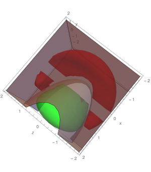
Figure 2: Example 2. (Red region: $P_{x,y,z}(\phi(x,y,z,a_{1},b_{1},c_{1},d_{1}))$; Green region: $P_{x,y,z}(\psi(x,y,z,a_{2},b_{2},c_{2},d_{2}))$; Gray region: $\{(x,y,z)\mid h(x,y,z)>0\}$.)

Consider two contradictory formulas $\phi$ and $\psi$ as follows: $\phi(x,y,z$, $a_{1}$, $b_{1},c_{1},d_{1}):$

$$f_{1}(x,y,z,a_{1},b_{1},c_{1},d_{1})\geq 0~{}~{}\wedge$$

$$f_{2}(x,y,z,a_{1},b_{1},c_{1},d_{1})\geq 0~{}~{}\wedge$$

$$f_{3}(x,y,z,a_{1},b_{1},c_{1},d_{1})\geq 0$$

and $\psi(x,y,z,a_{2},b_{2},c_{2},d_{2}):$

$$g_{1}(x,y,z,a_{2},b_{2},c_{2},d_{2})\geq 0~{}~{}\wedge$$

$$g_{2}(x,y,z,a_{2},b_{2},c_{2},d_{2})\geq 0~{}~{}\wedge$$

$$g_{3}(x,y,z,a_{2},b_{2},c_{2},d_{2})\geq 0,$$

where

$$f_{1}=4-x^{2}-y^{2}-z^{2}-a_{1}^{2}-b_{1}^{2}-c_{1}^{2}-d_{1}^{2},$$

$$f_{2}=-y^{4}+2x^{4}-a_{1}^{4}-1/100,$$

$$f_{3}=z^{2}-b_{1}^{2}-c_{1}^{2}-d_{1}^{2}-x-1,$$

$$g_{1}=4-x^{2}-y^{2}-z^{2}-a_{2}^{2}-b_{2}^{2}-c_{2}^{2}-d_{2}^{2},$$

$$g_{2}=x^{2}-y-a_{2}-b_{2}-d_{2}^{2}-3,$$

$$g_{3}=x.$$

It is easy to observe that $\phi$ and $\psi$ satisfy the conditions in Problem 1. Since there are local variables in $\phi$ and $\psi$ and the degree of $f_{2}$ is $4$, the interpolant generation methods in DXZ13 and GDX16 are not applicable. We get a concrete ${\rm SDP}$ problem of the form (11) by setting the degree of the polynomial $h(x,y,z)$ in (11) to be $2$. Using the MATLAB package YALMIP lofberg2004 and Mosek mosek2015mosek , we obtain

$$h(x,y,z)=-416.7204-914.7840x+472.6184y$$

$$\quad+199.8985x^{2}+190.2252y^{2}+690.4208z^{2}-187.1592xy.$$

Pictorially, we plot $P_{x,y,z}(\phi(x,y,z,a_{1},b_{1},c_{1},d_{1}))$, $P_{x,y,z}(\psi(x,y,z,a_{2},b_{2},c_{2},$ $d_{2}))$ and $\{(x,y,z)\mid h(x,y,z)>0\}$ in Fig. 2. It is evident that $h(x,y,z)$ as presented above for $d_{h}=2$ is a real interpolant for $\phi(x,y,z,a,b,c,d)$ and $\psi(x,y,z,a,b,c,d)$.

5 Avoidance of the unsoundness due to numerical error in SDP

To the best of our knowledge, all the efficient SDP solvers are based on interior point method, which is a numerical method. Thus, the numerical error is inevitable in our approach. In this section, we discuss how to avoid the unsoundness of our approach caused by numerical error in SDP based on the work in RVS16 .

We say a square matrix $A$ is positive semidefinite is $A$ is real symmetric and all eigenvalues of $A$ are $\geq 0$, denote $A\succeq 0$ for $A$ is positive semidefinite.

In order to solve formula (11) to obtain $h(\mathbf{x})$, we first need to fix a degree bound of $u_{i}$, $v_{j}$ and $h$, say $2d$, $d\in\mathbb{N}$. It is well-known that any $u(\mathbf{x})\in\sum\mathbb{R}[\mathbf{x}]^{2}$ with degree $2d$ can be represented by

$$u(\mathbf{x})\equiv E_{d}(\mathbf{x})^{T}C_{u}E_{d}(\mathbf{x}),$$ (12)

where $C_{u}\in\mathbb{R}^{\binom{r+d}{d}\times\binom{r+d}{d}}$ with $C_{u}\succeq 0$, $E_{d}(\mathbf{x})$ is a column vector with all monomials in $\mathbf{x}$, whose total degree is not greater than $d$, and $E_{d}(\mathbf{x})^{T}$ stands for the transposition of $E_{d}(\mathbf{x})$. Equaling the corresponding coefficient of each monomial whose degree is less than or equal to $2d$ at the two sides of (12), we can get a linear equation system of the form

$$\mathtt{tr}(A_{u,k}C_{u})=b_{u,k},~{}k=1,\ldots,K_{u},$$ (13)

where $A_{u,k}\in\mathbb{R}^{\binom{r+d}{d}\times\binom{r+d}{d}}$ is constant matrix, $b_{u,k}\in\mathbb{R}$ is constant, $\mathtt{tr}(A)$ stands for the trace of matrix $A$. Thus, searching for $u_{i}$, $v_{j}$ and $h$ satisfying (11) can be reduced to the following SDP problem:

$$\begin{split}\mathtt{find}:~{}&C_{u_{1}},\ldots,C_{u_{m}},C_{v_{1}},\ldots,C_{v_{n}},C_{h},\\ \mathtt{s.t.}~{}&\mathtt{tr}(A_{u_{i},k}C_{u_{i}})=b_{u_{i},k},~{}i=1,\ldots,m,k=1,\ldots,K_{u_{i}},\\ &\mathtt{tr}(A_{v_{j},k}C_{v_{j}})=b_{v_{j},k},~{}j=1,\ldots,n,k=1,\ldots,K_{v_{j}},\\ &\mathtt{tr}(A_{h,k}C_{h})=b_{h,k},~{}k=1,\ldots,K_{h},\\ &\mathtt{diag}(C_{u_{1}},\ldots,C_{u_{m}},C_{v_{1}},\ldots,C_{v_{n}},C_{h-1-uf},C_{-h-1-vg})\succeq 0,\end{split}$$ (14)

where $C_{h-1-uf}$ is the matrix corresponding to polynomial $h-1-\sum_{i=1}^{m}u_{i}f_{i}$, which is a linear combination of $C_{u_{1}}$, …, $C_{u_{m}}$ and $C_{h}$; similarly, $C_{-h-1-vg}$ is the matrix corresponding to polynomial $-h-1-\sum_{j=1}^{n}v_{j}g_{j}$, which is a linear combination of $C_{v_{1}}$, …, $C_{v_{n}}$ and $C_{h}$; and $\mathtt{diag}(C_{1},\ldots,C_{k})$ is a block-diagonal matrix of $C_{1},\ldots,C_{k}$.

Let $D$ be the dimension of $C=\mathtt{diag}(C_{u_{1}},\ldots,$ $C_{-h-1-vg})$, i.e., $\mathtt{diag}(C_{u_{1}}$, …, $C_{-h-1-vg})\in\mathbb{R}^{D\times D}$ and $\widehat{C}$ be the approximate solution to (14) returned by calling a numerical SDP solver, the following theorem is proved in RVS16 .

Theorem 5.1 (RVS16 , Theorem 3)

$C\succeq 0$ if there exists $\widetilde{C}\in\mathbb{F}^{D\times D}$ such that the following conditions hold:

• $\widetilde{C}_{ij}=C_{ij}$, for any $i\neq j$;

• $\widetilde{C}_{ii}\leq C_{ii}-\alpha$, for any $i$; and

• the Cholesky algorithm implemented in floating-point arithmetic can conclude that $\widetilde{C}$ is positive semi-definite,

where $\mathbb{F}$ is a floating-point format, $\alpha=\frac{(D+1)\kappa}{1-(2D+2)\kappa}\mathtt{tr}(C)+4(D+1)(2(D+2)+\max_{i}\{C_{ii}\})\eta$, in which $\kappa$ is the unit roundoff of $\mathbb{F}$ and $\eta$ is the underflow unit of $\mathbb{F}$.

Corollary 2

Let $\widetilde{C}\in\mathbb{F}^{D\times D}$. Suppose that $\frac{(D+1)D\kappa}{1-(2D+2)\kappa}+4(D+1)\eta\leq\frac{1}{2}$, $\beta=\frac{(D+1)\kappa}{1-(2D+2)\kappa}\mathtt{tr}(\widetilde{C})+4(D+1)(2(D+2)+\max_{i}\{\widetilde{C}_{ii}\})\eta>0$, where $\mathbb{F}$ is a floating-point format. Then $\widetilde{C}+2\beta I\succeq 0$ if the Cholesky algorithm based on floating-point arithmetic succeeds on $\widetilde{C}$, i.e., concludes that $\widetilde{C}$ is positive semi-definite.

Proof (of Corollary 2)

By directly checking.

According to Remark 5 in RVS16 , for IEEE 754 binary64 format with rounding to nearest, $\kappa=2^{-53}(\simeq 10^{-16})$ and $\eta=2^{-1075}(\simeq 10^{-323})$. In this case, the order of magnitude of $\beta$ is $10^{-10}$ and $\frac{(D+1)D\kappa}{1-(2D+2)\kappa}+4(D+1)\eta$ is $10^{-13}$, much less than $\frac{1}{2}$. Obviously, $\beta$ becomes smaller when the length of binary format becomes longer.

Without loss of generality, we suppose that the Cholesky algorithm succeed on $\widehat{C}$ the solution of (14), which is reasonable since if an SDP solver returns a solution $\widehat{C}$, then $\widehat{C}$ should be considered to be positive semi-definite in a perspective of numeric computation (in other words, we assume the answer obtained by numeric computation is correct.).

Therefore, by Corollary 2, we have $\widehat{C}+2\beta I\succeq 0$ holds, where $I$ is the identity matrix with corresponding dimension. Then we have

$$\mathtt{diag}(\widehat{C}_{u_{1}},\ldots,\widehat{C}_{u_{m}},\widehat{C}_{v_{1}},\ldots,\widehat{C}_{v_{n}},\widehat{C}_{h-1-uf},\widehat{C}_{-h-1-vg})$$

$$+2\beta I\succeq 0,$$

i.e.,

$$\begin{split}&\widehat{C}_{u_{1}}+2\beta I\succeq 0,~{}\ldots,~{}\widehat{C}_{u_{m}}+2\beta I\succeq 0,\\ &\widehat{C}_{v_{1}}+2\beta I\succeq 0,~{}\ldots,~{}\widehat{C}_{v_{n}}+2\beta I\succeq 0,\\ &\widehat{C}_{h-1-uf}+2\beta I\succeq 0,~{}\widehat{C}_{-h-1-vg}+2\beta I\succeq 0.\end{split}$$ (15)

Let $\epsilon=\max_{p\in P,1\leq i\leq K_{p}}|\mathtt{tr}(A_{p,i}\widehat{C}_{p})-b_{p,i}|$, where $P=\{u_{1},\ldots,u_{m},v_{1},\ldots,v_{n},h\}$, which can be regarded as the tolerance of the SDP solver. Since $|\mathtt{tr}(A_{p,i}C_{p})-b_{p,i}|$ is the error term for each monomial of $p$, i.e., $\epsilon$ can be considered as the error bound on the coefficients of polynomials $u_{i}$, $v_{j}$ and $h$, for any polynomial $\hat{u_{i}}$ ( $\hat{v_{j}}$ and $\hat{h}$), computed from (13) by replacing $C_{u}$ with the corresponding $\widehat{C_{u}}$, there exists a corresponding remainder term $R_{u_{i}}$ (resp. $R_{v_{j}}$ and $R_{h}$) with degree not greater than $2d$, whose coefficients are bounded by $\epsilon$. Hence, from (15), we have

$$\begin{split}\widehat{u_{i}}+R_{u_{i}}+2\beta E_{d}(\mathbf{x},\mathbf{y})^{T}E_{d}(\mathbf{x},\mathbf{y})\in\sum\mathbb{R}[\mathbf{x},\mathbf{y}]^{2},\\ i=1,\ldots,m,\\ \widehat{v_{j}}+R_{v_{j}}+2\beta E_{d}(\mathbf{x},\mathbf{z})^{T}E_{d}(\mathbf{x},\mathbf{z})\in\sum\mathbb{R}[\mathbf{x},\mathbf{z}]^{2},\\ j=1,\ldots,n,\\ \widehat{h}+R_{h}-1-\sum_{i=1}^{m}(\widehat{u_{i}}+R^{\prime}_{u_{i}})f_{i}+2\beta E_{d}(\mathbf{x},\mathbf{y})^{T}E_{d}(\mathbf{x},\mathbf{y})\in\sum\mathbb{R}[\mathbf{x},\mathbf{y}]^{2},\\ -\widehat{h}+R^{\prime}_{h}-1-\sum_{j=1}^{m}(\widehat{v_{j}}+R^{\prime}_{v_{j}})g_{j}+2\beta E_{d}(\mathbf{x},\mathbf{z})^{T}E_{d}(\mathbf{x},\mathbf{z})\in\sum\mathbb{R}[\mathbf{x},\mathbf{z}]^{2}.\end{split}$$ (16)

Now, in order to avoid unsoundness of our approach caused by the numerical issue due to SDP, we have to prove

$$f_{1}\geq 0\wedge\cdots\wedge f_{m}\geq 0\Rightarrow\widehat{h}>0,$$ (17)

$$g_{1}\geq 0\wedge\cdots\wedge g_{n}\geq 0\Rightarrow\widehat{h}<0.$$ (18)

Regarding (17), let $R_{2d,\mathbf{x}}$ be a polynomial in $\mathbb{R}[|\mathbf{x}|]$, whose total degree is $2d$, and all coefficients are $1$, e.g., $R_{2,x,y}=1+|x|+|y|+|x^{2}|+|xy|+|y^{2}|$. Since $S=\{(\mathbf{x},\mathbf{y})\mid f_{1}\geq 0\wedge\cdots\wedge f_{m}\geq 0\}$ is a compact set, then for any polynomial $p\in\mathbb{R}[\mathbf{x},\mathbf{y}]$, $|p|$ is bounded on $S$. Let $M_{1}$ be an upper bound of $R_{2d,\mathbf{x},\mathbf{y}}$ on $S$, $M_{2}$ an upper bound of $E_{d}(\mathbf{x},\mathbf{y})^{T}E_{d}(\mathbf{x},\mathbf{y})$, and $M_{f_{i}}$ an upper bound of $f_{i}$ on $S$. Then, $|R_{u_{i}}|$, $|R^{\prime}_{u_{i}}|$ and $|R_{h}|$ are bounded by $\epsilon M_{1}$. Let $E_{\mathbf{x}\mathbf{y}}=E_{d}(\mathbf{x},\mathbf{y})^{T}E_{d}(\mathbf{x},\mathbf{y})$. So for any $(\mathbf{x}_{0},\mathbf{y}_{0})\in S$, considering the polynomials below at $(\mathbf{x}_{0},\mathbf{y}_{0})\in S$, by the first and third line in (16), we have

$$\widehat{h}\geq 1-R_{h}+\sum_{i=1}^{m}(\widehat{u_{i}}+R^{\prime}_{u_{i}})f_{i}-2\beta E_{\mathbf{x}\mathbf{y}}$$

$$\geq 1-\epsilon M_{1}+\sum_{i=1}^{m}(\widehat{u_{i}}+R_{u_{i}}+2\beta E_{\mathbf{x}\mathbf{y}}+R^{\prime}_{u_{i}}-R_{u_{i}}-2\beta E_{xy})f_{i}-2\beta M_{2}$$

$$= 1-\epsilon M_{1}-2\beta M_{2}+\sum_{i=1}^{m}(\widehat{u_{i}}+R_{u_{i}}+2\beta E_{\mathbf{x}\mathbf{y}})f_{i}+\sum_{i=1}^{m}(R^{\prime}_{u_{i}}-R_{u_{i}}-2\beta E_{\mathbf{x}\mathbf{y}})f_{i}$$

$$\geq 1-\epsilon M_{1}-2\beta M_{2}+0-\sum_{i=1}^{m}(\epsilon M_{1}+\epsilon M_{1}+2\beta M_{2})M_{f_{i}}$$

$$= 1-(2\sum_{i=1}^{m}M_{f_{i}}+1)M_{1}\epsilon-2(\sum_{i=1}^{m}M_{f_{i}}+1)M_{2}\beta.$$

Whence,

$$\begin{split}&f_{1}\geq 0\wedge\cdots\wedge f_{m}\geq 0\Rightarrow\\ &\widehat{h}\geq 1-(2\sum_{i=1}^{m}M_{f_{i}}+1)M_{1}\epsilon-2(\sum_{i=1}^{m}M_{f_{i}}+1)M_{2}\beta.\end{split}$$ (19)

Let $S^{\prime}=\{(\mathbf{x},\mathbf{z})\mid g_{1}\geq 0\wedge\cdots\wedge g_{n}\geq 0\}$, $M_{3}$ be an upper bound of $R_{2d,\mathbf{x},\mathbf{z}}$ on $S^{\prime}$, $M_{4}$ an upper bound of $E_{d}(\mathbf{x},\mathbf{z})^{T}E_{d}(\mathbf{x},\mathbf{z})$ on $S^{\prime}$, and $M_{g_{j}}$ an upper bound of $g_{j}$ on $S^{\prime}$. Similarly to the above, it follows

$$g_{1}\geq 0\wedge\cdots\wedge g_{n}\geq 0\Rightarrow$$

$$-\widehat{h}\geq 1-(2\sum_{j=1}^{n}M_{g_{j}}+1)M_{3}\epsilon-2(\sum_{j=1}^{n}M_{g_{j}}+1)M_{4}\beta.$$

So, the following proposition holds.

Proposition 2

There exist two positive constants $\gamma_{1}$ and $\gamma_{2}$ such that

$$f_{1}\geq 0\wedge\cdots\wedge f_{m}\geq 0\Rightarrow\widehat{h}\geq 1-\gamma_{1}\epsilon-\gamma_{2}\beta,$$ (20)

$$g_{1}\geq 0\wedge\cdots\wedge g_{n}\geq 0\Rightarrow-\widehat{h}\geq 1-\gamma_{1}\epsilon-\gamma_{2}\beta.$$ (21)

Proof (of Proposition 2)

We just need to take

$$\gamma_{1}=\max((2\sum_{i=1}^{m}M_{f_{i}}+1)M_{1},(2\sum_{j=1}^{n}M_{g_{j}}+1)M_{3})\,,$$

$$\gamma_{2}=\max(2(\sum_{i=1}^{m}M_{f_{i}}+1)M_{2},2(\sum_{j=1}^{n}M_{g_{j}}+1)M_{4})$$

in formulas (19) and (5).

Since $\epsilon$ and $\beta$ heavily rely on the numerical tolerance and the floating point representation, it is easy to see that $\epsilon$ and $\beta$ become small enough with $\gamma_{1}\epsilon<\frac{1}{2}$ and $\gamma_{2}\beta<\frac{1}{2}$, if the numerical tolerance is small enough and the length of the floating point representation is long enough. This implies that

$$f_{1}\geq 0\wedge\cdots\wedge f_{m}\geq 0\Rightarrow\widehat{h}>0,$$

$$g_{1}\geq 0\wedge\cdots\wedge g_{n}\geq 0\Rightarrow-\widehat{h}>0.$$

If so, any numerical result $\widehat{h}>0$ returned by calling an SDP solver to (14) is guaranteed to be a real interpolant for $\phi$ and $\psi$, i.e., a correct solution to Problem 1.

Example 3

Consider the numerical result for Example 2 in Section 4. Let $M_{f_{1}}$, $M_{f_{2}}$, $M_{f_{3}}$, $M_{g_{1}}$, $M_{g_{2}}$, $M_{g_{3}}$, $M_{1}$, $M_{2}$, $M_{3}$, $M_{4}$ are defined as above. It is easy to see that

$$f_{1}\geq 0\Rightarrow |x|\leq 2\wedge|y|\leq 2\wedge|z|\leq 2\wedge|a_{1}|\leq 2\wedge|b_{1}|\leq 2\wedge|c_{1}|\leq 2\wedge|d_{1}|\leq 2.$$

Then, by simple calculations, we obtain

$$M_{f_{1}}=4,M_{f_{2}}=32,M_{f_{3}}=3,M_{1}=83,M_{2}=29.$$

Thus,

$$(2\sum_{i=1}^{m}M_{f_{i}}+1)M_{1}=6557,\quad 2(\sum_{i=1}^{m}M_{f_{i}}+1)M_{2}=2320.$$

Also, since

$$g_{1}\geq 0\Rightarrow |x|\leq 2\wedge|y|\leq 2\wedge|z|\leq 2\wedge|a_{2}|\leq 2\wedge|b_{2}|\leq 2\wedge|c_{2}|\leq 2\wedge|d_{2}|\leq 2,$$

we obtain

$$M_{g_{1}}=4,M_{g_{2}}=7,M_{g_{3}}=2,M_{3}=83,M_{4}=29.$$

Thus,

$$(2\sum_{i=1}^{m}M_{g_{i}}+1)M_{3}=2241,\quad 2(\sum_{i=1}^{m}M_{g_{i}}+1)M_{4}=812.$$

Consequently, we have $\gamma_{1}=6557$ and $\gamma_{2}=2320$ in Proposition 2.

Due to the fact that the default error tolerance is $10^{-8}$ in the SDP solver Mosek and $h$ is rounding to $4$ decimal places, we have $\epsilon=\frac{10^{-4}}{2}$. In addition, as the absolute value of each element in $\widehat{C}$ is less than $10^{3}$, and the dimension of $D$ is less than $10^{3}$, we obtain that

$$\beta =\frac{(D+1)\kappa}{1-(2D+2)\kappa}\mathtt{tr}(\widetilde{C})+4(D+1)(2(D+2)+\max_{i}(\widetilde{C}_{ii}))\eta$$

$$\leq\frac{(1000+1)10^{-16}}{1-(2000+2)10^{-16}}10^{6}+4(1000+1)(2(1000+2)+1000)10^{-1075}$$

$$\leq 10^{-6}.$$

Consequently,

$$\gamma_{1}\epsilon\leq 6557\cdot\frac{10^{-4}}{2}<\frac{1}{2},$$

$$\gamma_{2}\beta\leq 2320\cdot 10^{-6}<\frac{1}{2},$$

which imply that $h(x,y,z)>0$ presented in Example 2 is indeed a sound interpolant.

Remark 1

Besides, the result could be verified by the following symbolic computation procedure instead: computing $P_{\mathbf{x}}(\phi)$ and $P_{\mathbf{x}}(\psi)$ first by some symbolic tools, such as Redlog dolzmann1997 which is a package that extends the computer algebra system REDUCE to a computer logic system; then verifying $\mathbf{x}\in P_{\mathbf{x}}(\phi)\Rightarrow h(\mathbf{x})>0$ and $\mathbf{x}\in P_{\mathbf{x}}(\psi)\Rightarrow h(\mathbf{x})<0.$ For this example, $P_{x,y,z}(\phi)$ and $P_{x,y,z}(\psi)$ obtained by Redlog are too complicated and therefore not presented here. The symbolic computation can verify that $h(x,y,z)$ in this example is exactly an interpolant, which confirms our conclusion.

6 Generalizing to general polynomial formulas

Problem 2

Let $\phi(\mathbf{x},\mathbf{y})$ and $\psi(\mathbf{x},\mathbf{z})$ be two polynomial formulas defined as follows,

$$\phi(\mathbf{x},\mathbf{y}):\bigvee_{i=1}^{m}\phi_{i},\quad\phi_{i}=\bigwedge_{k=1}^{K_{i}}f_{i,k}(\mathbf{x},\mathbf{y})\geq 0;$$

$$\psi(\mathbf{x},\mathbf{z}):\bigvee_{j=1}^{n}\psi_{j},\quad\psi_{j}=\bigwedge_{s=1}^{S_{j}}g_{j,s}(\mathbf{x},\mathbf{z})\geq 0,$$

where all $f_{i,k}$ and $g_{j,s}$ are polynomials. Suppose $\phi\wedge\psi\models\bot$, and for $i=1,\ldots,m$, $j=1,\ldots,n$, $\{(\mathbf{x},\mathbf{y})\mid\phi_{i}(\mathbf{x},\mathbf{y})\}$ and $\{(\mathbf{x},\mathbf{z})\mid\psi_{j}(\mathbf{x},\mathbf{z})\}$ are all semi-algebraic sets of the Archimedean form. Find a polynomial $h(\mathbf{x})$ such that $h(\mathbf{x})>0$ is an interpolant for $\phi$ and $\psi$.

Theorem 6.1

For Problem 2, there exists a polynomial $h(\mathbf{x})$ satisfying

$$\forall\mathbf{x}\in P_{\mathbf{x}}(\phi(\mathbf{x},\mathbf{y})),h(\mathbf{x})>0,$$

$$\forall\mathbf{x}\in P_{\mathbf{x}}(\psi(\mathbf{x},\mathbf{z})),h(\mathbf{x})<0.$$

Proof (of Theorem 6.1)

We claim that Lemma 1 holds for Problem 2 as well. Since $\{(\mathbf{x},\mathbf{y})\mid\phi_{i}(\mathbf{x},\mathbf{y})\}$ and $\{(\mathbf{x},\mathbf{z})\mid\psi_{j}(\mathbf{x},\mathbf{z})\}$ are all semi-algebraic sets of the Archimedean form, then $\{(\mathbf{x},\mathbf{y})\mid\phi(\mathbf{x},\mathbf{y})\}$ and $\{(\mathbf{x},\mathbf{z})\mid\psi(\mathbf{x},\mathbf{z})\}$ both are compact. See $\{(\mathbf{x},\mathbf{y})\mid\phi(\mathbf{x},\mathbf{y})\}$ or $\{(\mathbf{x},\mathbf{z})\mid\psi(\mathbf{x},\mathbf{z})\}$ as $S$ in the proof of Lemma 1, then Lemma 1 holds for Problem 2. Thus, the rest of proof is same as that for Theorem 3.2.

Corollary 3

Let $\phi(\mathbf{x},\mathbf{y})$ and $\psi(\mathbf{x},\mathbf{z})$ be defined as in Problem 2. There must exist a polynomial $h(\mathbf{x})$ such that $h(\mathbf{x})>0$ is an interpolant for $\phi$ and $\psi$.

Theorem 6.2

Let $\phi(\mathbf{x},\mathbf{y})$ and $\psi(\mathbf{x},\mathbf{z})$ be defined as in Problem 2. Then there exists a polynomial $h(\mathbf{x})$ and $\sum_{i=1}^{m}(K_{i}+1)+\sum_{j=1}^{n}(S_{j}+1)$ sum of squares polynomials $u_{i,k}(\mathbf{x},\mathbf{y})$ $(i=1,\ldots,m$, $k=1,\ldots,K_{i}+1)$, $v_{j,s}(\mathbf{x},\mathbf{z})$ $(j=1,\ldots,n$, $s=1,\ldots,S_{j})$ satisfying the following semi-definite constraints such that $h(\mathbf{x})>0$ is an interpolant for $\phi(\mathbf{x},\mathbf{y})$ and $\psi(\mathbf{x},\mathbf{z})$:

$$h-1=\sum_{k=1}^{K_{i}}u_{i,k}f_{i,k}+u_{i,K_{i}+1},\quad i=1,\ldots,m;$$ (22)

$$-h-1=\sum_{s=1}^{S_{j}}v_{j,s}g_{j,s}+v_{j,S_{j}+1},\quad j=1,\ldots,n.$$ (23)

Proof (of Theorem 6.2)

According to the property of Archimedean, the proof is same as that for Theorem 4.1.

Similarly, Problem 2 can be equivalently reformulated as the problem of searching for sum of squares polynomials satisfying

$$\left\{\begin{split}&h(\mathbf{x})-1-\sum_{k=1}^{K_{i}}u_{i,k}f_{i,k}\in\sum\mathbb{R}[\mathbf{x},\mathbf{y}]^{2},i=1,\ldots,m;\\ &-h(\mathbf{x})-1-\sum_{s=1}^{S_{j}}v_{j,s}g_{j,s}\in\sum\mathbb{R}[\mathbf{x},\mathbf{z}]^{2},j=1,\ldots,n;\\ &u_{i,k}\in\sum\mathbb{R}[\mathbf{x},\mathbf{y}]^{2},i=1,\ldots,m,k=1,\ldots,K_{i};\\ &v_{j,s}\in\sum\mathbb{R}[\mathbf{x},\mathbf{z}]^{2},j=1,\ldots,n,s=1,\ldots,S_{j}.\end{split}\right.$$ (24)

Example 4

Consider

$$\phi(x,y,a_{1},a_{2},b_{1},b_{2}):(f_{1}\geq 0\wedge f_{2}\geq 0)\vee(f_{3}\geq 0\wedge f_{4}\geq 0),$$

$$\psi(x,y,c_{1},c_{2},d_{1},d_{2}):(g_{1}\geq 0\wedge g_{2}\geq 0)\vee(g_{3}\geq 0\wedge g_{4}\geq 0),$$

where

$$f_{1}= 16-(x+y-4)^{2}-16(x-y)^{2}-a_{1}^{2},$$

$$f_{2}= x+y-a_{2}^{2}-(2-a_{2})^{2},$$

$$f_{3}= 16-(x+y+4)^{2}-16(x-y)^{2}-b_{1}^{2},$$

$$f_{4}= -x-y-b_{2}^{2}-(2-b_{2})^{2},$$

$$g_{1}= 16-16(x+y)^{2}-(x-y+4)^{2}-c_{1}^{2},$$

$$g_{2}= y-x-c_{2}^{2}-(1-c_{2})^{2},$$

$$g_{3}= 16-16(x+y)^{2}-(x-y-4)^{2}-d_{1}^{2},$$

$$g_{4}= x-y-d_{2}^{2}-(1-d_{2})^{2}.$$

We get a concrete ${\rm SDP}$ problem of the form (24) by setting the degree of $h(x,y)$ in (24) to be $2$. Using the MATLAB package YALMIP and Mosek, we obtain

$$h(x,y)=-2.3238+0.6957x^{2}+0.6957y^{2}+7.6524xy.$$

The result is plotted in Fig. LABEL:fig317, and can be verified either by numerical error analysis as in Example 2 or by a symbolic procedure like REDUCE as described in Remark 1.

Example 5 (Ultimate)

Let

$$\phi=(f_{1}\geq 0\wedge f_{2}\geq 0\vee f_{3}\geq 0)\wedge f_{4}\geq 0\wedge f_{5}\geq 0\vee f_{6}\geq 0,$$

$$\psi=(g_{1}\geq 0\wedge g_{2}\geq 0\vee g_{3}\geq 0)\wedge g_{4}\geq 0\wedge g_{5}\geq 0\vee g_{6}\geq 0,$$

where

$$f_{1} = 3.8025-x^{2}-y^{2},$$

$$f_{2} = y,$$

$$f_{3} = 0.9025-(x-1)^{2}-y^{2},$$

$$f_{4} = (x-1)^{2}+y^{2}-0.09,$$

$$f_{5} = (x+1)^{2}+y^{2}-1.1025,$$

$$f_{6} = 0.04-(x+1)^{2}-y^{2},$$

$$g_{1} = 3.8025-x^{2}-y^{2},$$

$$g_{2} = -y,$$

$$g_{3} = 0.9025-(x+1)^{2}-y^{2},$$

$$g_{4} = (x+1)^{2}+y^{2}-0.09,$$

$$g_{5} = (x-1)^{2}+y^{2}-1.1025,$$

$$g_{6} = 0.04-(x-1)^{2}-y^{2}.$$

We first convert $\phi$ and $\psi$ to the disjunction normal form as:

$$\phi= (f_{1}\geq 0\wedge f_{2}\geq 0\wedge f_{4}\geq 0\wedge f_{5}\geq 0)$$

$$\vee(f_{3}\geq 0\wedge f_{4}\geq 0\wedge f_{5}\geq 0)\vee(f_{6}\geq 0),$$

$$\psi= (g_{1}\geq 0\wedge g_{2}\geq 0\wedge g_{4}\geq 0\wedge g_{5}\geq 0)$$

$$\vee(g_{3}\geq 0\wedge g_{4}\geq 0\wedge g_{5}\geq 0)\vee(g_{6}\geq 0).$$

We get a concrete ${\rm SDP}$ problem of the form (24) by setting the degree of $h(x,y)$ in (24) to be $7$. Using the MATLAB package YALMIP and Mosek, keeping the decimal to four, we obtain

$$h (x,y)=1297.5980x+191.3260y-3172.9653x^{3}+196.5763x^{2}y$$

$$+2168.1739xy^{2}+1045.7373y^{3}+1885.8986x^{5}-1009.6275x^{4}y$$

$$+3205.3793x^{3}y^{2}-1403.5431x^{2}y^{3}+1842.0669xy^{4}$$

$$+1075.2003y^{5}-222.0698x^{7}+547.9542x^{6}y-704.7474x^{5}y^{2}$$

$$+1724.7008x^{4}y^{3}-728.2229x^{3}y^{4}+1775.7548x^{2}y^{5}$$

$$-413.3771xy^{6}+1210.2617y^{7}.$$

The result is plotted in Fig. LABEL:ultimate, and can be verified either by numerical error analysis as in Example 2 or by a symbolic procedure like REDUCE as described in Remark 1.

7 Application to Invariant Generation

In this section, as an application, we show how to apply our approach to invariant generation in program verification.

In LSXLSH2017 , Lin et al. proposed a framework for invariant generation using weakest precondition, strongest postcondition and interpolation, which consists of two procedures, i.e., synthesizing invariants by forward interpolation based on strongest postcondition and interpolant generation, and by backward interpolation based on weakest precondition and interpolant generation. In LSXLSH2017 , only linear invariants can be synthesized as no powerful approaches are available to synthesize nonlinear interpolants. Obviously, our results can strengthen their framework by allowing to generate nonlinear invariants. To this end, we revise the two procedures, i.e., Squeezing Invariant - Forward and Squeezing Invariant - Backward, in their framework accordingly, and obtain Algorithm 1 and Algorithm 2. The major revisions include:

• firstly, we exploit our method to synthesize interpolants see line 4 in Algorithm 1 and line 4 in in Algorithm 2;

• secondly, we add a conditional statement for $A_{i+1}$ at line 7-10 in Algorithm 1 in order to make $A_{i+1}$ to be Archimedean, the same for $B_{j+1}$ in Algorithm 2.

We then illustrate the basic idea by exploiting Algorithm 1 to an example given in Algorithm 3. The reader can refer to LSXLSH2017 for the detail of the framework.

Algorithm 1 Revised Squeezing Invariant - Forward

0:  An annotated loop: $\{P\}$ while $\rho$ do $C$ $\{Q\}$

0:   (yes/no, $\mathcal{I}$), where $\mathcal{I}$ is a loop invariant

1:  $A_{0}\leftarrow P$; $B_{0}\leftarrow(\neg\rho\wedge\neg Q)$; $i\leftarrow 0$; $j\leftarrow 0$;

2:  while $\top$ do

3:     if $(\bigvee_{k=0}^{i}A_{i})\wedge B_{j}$ is not satisfiable then

4:        call our method to synthesize an interpolant for $(\bigvee_{k=0}^{i}A_{i})$ and $B_{j}$, say $\mathcal{I}_{i}$; {Use our method to generate interpolant}

5:        if $\{\mathcal{I}_{i}\wedge\rho\}\,C\,\{\mathcal{I}_{i}\}$ then

6:           return  (yes, $\mathcal{I}_{i}$);

7:        else if $\mathcal{I}_{i}$ is bounded then

8:           $A_{i+1}\leftarrow\mathsf{sp}(\mathcal{I}_{i}\wedge\rho,C)$;

9:        else

10:           $A_{i+1}\leftarrow\mathsf{sp}(A_{i}\wedge\rho,C)$;

11:        end if{$\mathsf{sp}$: a predicate transformer to compute the strongest postcondition of $C$ w.r.t. $\mathcal{I}_{i}\wedge\rho$}

12:        $i\leftarrow i+1$;

13:        $B_{j+1}\leftarrow B_{0}\vee(\rho\wedge\mathsf{wp}(C,B_{j}))$; {$\mathsf{wp}$: a predicate transformer to compute the weakest precondition of $C$ w.r.t. $B_{j}$}

14:        $i\leftarrow i+1$;

15:     else if $A_{i}$ is concrete then

16:        return  (no, $\bot$);

17:     else

18:        while $A_{i}$ is not concrete do

19:           $i\leftarrow i-1$;

20:        end while

21:        $A_{i+1}\leftarrow\mathsf{sp}(A_{i}\wedge\rho,C)$;

22:        $i\leftarrow i+1$;

23:     end if

24:  end while

Algorithm 2 Revised Squeezing Invariant - Backward

0:  An annotated loop: $\{P\}$ while $\rho$ do $C$ $\{Q\}$

0:   (yes/no, $\mathcal{I}$), where $\mathcal{I}$ is a loop invariant

1:  $A_{0}\leftarrow P$; $B_{0}\leftarrow(\neg\rho\wedge\neg Q)$; $i\leftarrow 0$; $j\leftarrow 0$;

2:  while $\top$ do

3:     if $B_{j}\wedge(\bigvee_{k=0}^{i}A_{i})$ is not satisfiable then

4:        call our method to synthesize an interpolant for $B_{j}\wedge(\bigvee_{k=0}^{i}A_{i})$, say $I_{j}$; {Use our method to generate interpolant}

5:        if $\{\neg\mathcal{I}_{j}\wedge\rho\}C\{\neg\mathcal{I}_{j}\}$ then

6:           return  (yes, $\neg\mathcal{I}_{j}$);

7:        else if $\mathcal{I}_{j}$ is bounded then

8:           $B_{j+1}\leftarrow\mathcal{I}_{j}\vee(\rho\wedge\mathsf{wp}(C,\mathcal{I}_{j}))$;

9:        else

10:           $B_{j+1}\leftarrow B_{j}\vee(\rho\wedge\mathsf{wp}(C,B_{j}))$;

11:        end if

12:        $j\leftarrow j+1$;

13:        $A_{i+1}\leftarrow\mathsf{sp}(A_{i}\wedge\rho,C)$;

14:        $i\leftarrow i+1$;

15:     else if $B_{j}$ is concrete then

16:        return  (no, $\bot$);

17:     else

18:        while $B_{j}$ is not concrete do

19:           $j\leftarrow j-1$;

20:        end while

21:        $B_{j+1}\leftarrow B_{0}\vee(\rho\wedge\mathsf{wp}(C,B_{j}))$;

22:        $j\leftarrow j+1$;

23:     end if

24:  end while

Example 6

Consider a while loop given in Algorithm 3, which is adapted from DDLM13 by modifying the precondition and the postcondition so that the precondition and the negation of the postcondition are nonlinear and compact.

Algorithm 3

1:  /* Pre: $100-(x+50)^{2}\geq 0\wedge 100-y^{2}\geq 0$ */

2:  while $x<0$ do

3:     $x\leftarrow x+y$;

4:     $y\leftarrow y+1$;

5:  end while

6:  /* Post: $(x-5)^{2}+(y+3)^{4}>100$ */

We apply the algorithm Squeezing Invariant - Forward in Algorithm 1 to the loop to compute an invariant which can witness its correctness.

Firstly, at line 1 in Algorithm 1, we have $\rho:x<0$ and

$$A_{0}: ~{}100-(x+50)^{2}\geq 0\wedge 100-y^{2}\geq 0,$$

$$B_{0}: ~{}x\geq 0\wedge 100-(x-5)^{2}-(y+3)^{4}\geq 0.$$

Then, at line 3, $A_{0}\wedge B_{0}\models\bot$. Using our method, we can synthesize an interpolant for $A_{0}$ and $B_{0}$ (line 4) as:

$$\mathcal{I}_{0}: -4.8031-6.8601x+4.5900y+0.0905x^{2}-0.5331y^{2}$$

$$+0.1376xy>0.$$

It can be checked that $\{\mathcal{I}_{0}\wedge\rho\}\ C\ \{\mathcal{I}_{0}\}$ does not hold ( line 5), where $C$ stands for the loop body.

Secondly, since $\mathcal{I}_{0}$ is not bounded, set $A_{1}=\mathsf{sp}(A_{0}\wedge\rho,C)$ (line 10), and $B_{1}=B_{0}\vee(\rho\wedge\mathsf{wp}(C,B_{0}))$ (line 12), i.e.,

$$A_{1}: ~{}x=x^{\prime}+y^{\prime}\wedge y=y^{\prime}+1\wedge x^{\prime}<0\wedge 100-(x^{\prime}+50)^{2}\geq 0\wedge 100-y^{\prime 2}\geq 0,$$

$$B_{1}: ~{}B_{0}\vee(x<0\wedge x^{\prime\prime}=x+y\wedge y^{\prime\prime}=y+1\wedge x^{\prime\prime}\geq 0\wedge 100-x^{\prime\prime 2}-(y^{\prime\prime}+3)^{4}\geq 0).$$

Now, repeating the while loop once again, at line 3, we have $(A_{0}\vee A_{1})\wedge B_{1}$ is not satisfiable. Thus, with our method, we can obtain

$$\mathcal{I}_{1}: -5.5937-10.6412x+7.9251y+0.1345x^{2}+0.3086y^{2}+0.0020xy>0.$$

It can be checked that $\{\mathcal{I}_{1}\wedge\rho\}\ C\,\{\mathcal{I}_{1}\}$ holds. Thus, the algorithm will return $({\rm yes},\mathcal{I}_{1})$.

Since $\mathcal{I}_{1}$ is an interpolant of $(A_{0}\vee A_{1})\wedge B_{1}$, it follows that $(A_{0}\vee A_{1})\models\mathcal{I}_{1}$ and $\mathcal{I}_{1}\wedge B_{1}\models\bot$. From $(A_{0}\vee A_{1})\models\mathcal{I}_{1}$, we have $\mathrm{Pre}\models\mathcal{I}_{1}$ as $\mathrm{Pre}=A_{0}$. Moreover, from $\mathcal{I}_{1}\wedge B_{1}\models\bot$ and $B_{1}=B_{0}\vee(\rho\wedge\mathsf{wp}(C,B_{0}))$, we have $\mathcal{I}_{1}\wedge B_{0}\models\bot$, i.e., $\mathcal{I}_{1}\wedge(\neg\mathrm{Post}\wedge(\neg\rho))\models\bot$. This implies that $\mathcal{I}_{1}\wedge(\neg\rho)\models Q$. Hence, we have

$$\mathrm{Pre}\models\mathcal{I}_{1},~{}\mathcal{I}_{1}\wedge(\neg\rho)\models\mathrm{Post},~{}\{\mathcal{I}_{1}\wedge\rho\}\,C\,\{\mathcal{I}_{1}\},$$

i.e., $\mathcal{I}_{1}$ is an inductive invariant that can prove the correctness of the annotated loop in Algorithm 3.

Example 7

Consider another loop given in Algorithm 4 for controlling the acceleration of a car adapted from KB11 . Suppose we know that vc is in $[0,40]$ at the beginning of the loop, we would like to prove that $\textit{vc}<49.61$ holds after the loop. Since the loop guard is unknown, it means that the loop may terminate after any number of iterations.

Algorithm 4 Control code for accelerating a car

1:  /* Pre: $\textit{vc}\in[0,40]$ */

2:  while unknown do

3:     $\textit{fa}\leftarrow 0.5418*\textit{vc}*\textit{vc}$;

4:     $fr\leftarrow 1000-\textit{fa}$;

5:     $\textit{ac}\leftarrow 0.0005*fr$;

6:     $\textit{vc}\leftarrow\textit{vc}+\textit{ac}$;

7:  end while

8:  /* Post: $\textit{vc}<49.61$ */

We apply Algorithm 1 to the computation of an invariant to ensure that $\textit{vc}<49.61$ holds. Since vc is the velocity of car, $0\leq\textit{vc}<49.61$ is required to hold in order to maintain safety. Via Algorithm 1, we have $A_{0}=\{\textit{vc}\mid\textit{vc}(40-\textit{vc})\geq 0\}$ and $B=\{\textit{vc}\mid\textit{vc}<0\}\cup\{\textit{vc}\mid\textit{vc}\geq 49.61\}$. Here, we replace $B$ with $B^{\prime}=[-2,-1]\cup[49.61,55]$), which is in order to make $B$ to compact, i,e, $B^{\prime}=\{\textit{vc}\mid(\textit{vc}+2)(-1-\textit{vc})\geq 0\vee(\textit{vc}-49.61)(55-\textit{vc})\geq 0\}$, in order to make it with Archimedean form.

Firstly, it is evident that $A_{0}:\textit{vc}(40-\textit{vc})\geq 0$ implies $A_{0}\wedge B^{\prime}\models\bot$. By applying our approach, we obtain an interpolant

$$\mathcal{I}_{0}:1.4378+3.3947*\textit{vc}-0.083*\textit{vc}^{2}>0$$

for $A_{0}$ and $B^{\prime}$. It is verified that $\{\mathcal{I}_{0}\}\,C\,\{\mathcal{I}_{0}\}$ (line 5) does not hold, where $C$ stands for the loop body.

Secondly, by setting $A_{1}=sp(\mathcal{I}_{0},C)$ (line 8) and re-calling our approach, we obtain an interpolant

$$\mathcal{I}_{1}:2.0673+3.0744*\textit{vc}-0.0734*\textit{vc}^{2}>0$$

for $A_{0}\cup A_{1}$ and $B^{\prime}$. Likewise, it is verified that $\{\mathcal{I}_{1}\}\,C\,\{\mathcal{I}_{1}\}$ (line 5) does not hold.

Thirdly, repeating the above procedure again, we obtain an interpolant

$$\mathcal{I}_{2}:2.2505+2.7267*\textit{vc}-0.063*\textit{vc}^{2}>0,$$

and it is verified that $\{\mathcal{I}_{2}\}\,C\,\{\mathcal{I}_{2}\}$ holds, implying that $\mathcal{I}_{2}$ is an invariant. Moreover, it is trivial to verify that $\mathcal{I}_{2}\Rightarrow\textit{vc}<49.61$.

Consequently, we have the conclusion that $\mathcal{I}_{2}$ is an inductive invariant which witnesses the correctness of the loop.

8 Conclusion

In this paper we propose a sound and complete method to synthesize Craig interpolants for mutually contradictory polynomial formulas $\phi(\mathbf{x},\mathbf{y})$ and $\psi(\mathbf{x},\mathbf{z})$, with the form $f_{1}\geq 0\wedge\cdots\wedge f_{n}\geq 0$, where $f_{i}$’s are polynomials in $\mathbf{x},\mathbf{y}$ or $\mathbf{x},\mathbf{z}$ and the quadratic module generated by $f_{i}$’s is Archimedean. The interpolant could be generated by solving a semi-definite programming problem, which is a generalization of the method in DXZ13 dealing with mutually contradictory formulas with the same set of variables and the method in GDX16 dealing with mutually contradictory formulas with concave quadratic polynomial inequalities. As an application, we apply our approach to invariant generation in program verification.

As a future work, we would like to consider interpolant synthesizing for formulas with strict polynomial inequalities. Also, it deserves to consider how to synthesize interpolants for the combination of non-linear formulas and other theories based on our approach and other existing ones.

References

- (1) Benhamou, F., Granvilliers, L.: Continuous and interval constraints. In: Handbook of Constraint Programming, Foundations of Artificial Intelligence, vol. 2, pp. 571–603 (2006)
- (2) Bierstone, E., Milman, P.D.: Semianalytic and subanalytic sets. Publications Mathematiques de l’IHÉS 67, 5–42 (1988)
- (3) Bochnak, J., Coste, M., Roy, M.: Real Algebraic Geometry. Springer, (1998)
- (4) Borchers, B.: CSDP, a C library for semidefinite programming. Optimization Methods & Software 11(1-4), 613–623 (1999). http://projects.coin-or.org/csdp/
- (5) Cimatti, A., Griggio, A., Sebastiani, R.: Efficient interpolation generation in satisfiability modulo theories. In: TACAS 2008, Lecture Notes in Computer Science, vol. 4963, pp. 397–412 (2008)
- (6) Dai, L., Xia, B., Zhan, N.: Generating non-linear interpolants by semidefinite programming. In: CAV 2013, Lecture Notes in Computer Science, vol. 8044, pp. 364–380 (2013)
- (7) Dillig, I., Dillig, T., Li, B., Mcmillan, K.: Inductive invariant generation via abductive inference. ACM Sigplan Notices 48(10), 443–456 (2013)
- (8) Dolzmann, A., Sturm, T.: REDLOG: computer algebra meets computer logic. ACM Sigsam Bulletin 31(2), 2–9 (1997)
- (9) D’Silva, V., Purandare, M., Weissenbacher, G., Kroening, D.: Interpolant strength. In: VMCAI 2010, Lecture Notes in Computer Science, vol. 5944, pp. 129–145 (1997)
- (10) Gan, T., Dai, L., B, X., Zhan, N., Kapur, D., Chen, M.: Interpolation synthesis for quadratic polynomial inequalities and combination with EUF. In: IJCAR 2016, Lecture Notes in Computer Science, vol. 9706, pp. 195–212 (2016)
- (11) Gao, S., Kong, S., Clarke, E.M.: Proof generation from delta-decisions. In: SYNASC 2014, pp. 156–163 (2014)
- (12) Gao, S., Zufferey, D.: Interpolants in nonlinear theories over the reals. In: TACAS 2016, Lecture Notes in Computer Science, vol. 9636, pp. 625–641 (2016)
- (13) Graf, S., Saïdi, H.: Construction of abstract state graphs with PVS. In: CAV 1997, Lecture Notes in Computer Science, vol. 1254, pp. 72–83 (1997)
- (14) Henzinger, T., Jhala, R., Majumdar, R., McMillan, K.: Abstractions from proofs. In: POPL 2004, pp. 232–244 (2004)
- (15) Jung, Y., Lee, W., Wang, B., Yi, K.: Predicate generation for learning-based quantifier-free loop invariant inference. In: TACAS 2011, Lecture Notes in Computer Science, vol. 6605, pp. 205–219 (2011)
- (16) Kapur, D., Majumdar, R., Zarba, C.: Interpolation for data structures. In: FSE 2006, pp. 105–116 (2006)
- (17) Kovács, L., Voronkov, A.: Interpolation and symbol eleimination. In: CADE 2009, Lecture Notes in Computer Science, vol. 5663, pp. 199–213 (2009)
- (18) Krajíček, J.: Interpolation theorems, lower bounds for proof systems, and independence results for bounded arithmetic. J. of Symbolic Logic 62(2), 457–486 (1997)
- (19) Kupferschmid, S., Becker, B.: Craig interpolation in the presence of non-linear constraints. In: FORMATS’11, Lecture Notes in Computer Science, vol. 6919 (2011)
- (20) Lin, S., Sun, J., Xiao, H., Sanán, D., Hansen, H.: Fib: Squeezing loop invariants by interpolation between forward/backward predicate transformers. In: ASE2017, pp. 793–803 (2017)
- (21) Lofberg, J.: YALMIP: A toolbox for modeling and optimization in MATLAB. In: CACSD 2004, pp. 284–289. IEEE (2004)
- (22) Marshall, M.: Positive Polynomials and Sums of Squares. American Mathematical Society, (2008)
- (23) McMillan, K.: Interpolation and sat-based model checking. In: CAV 2003, Lecture Notes in Computer Science, vol. 3920, pp. 1–13 (2003)
- (24) McMillan, K.: An interpolating theorem prover. Theor. Comput. Sci. 345(1), 101–121 (2005)
- (25) McMillan, K.: Quantified invariant generation using interpolation saturation prover. In: TACAS 2008, Lecture Notes in Computer Science, vol. 4963, pp. 413–427 (2008)
- (26) Mosek, A.: The MOSEK optimization toolbox for MATLAB manual. Version 7.1 (Revision 28) p. 17 (2015)
- (27) Pudlǎk, P.: Lower bounds for resolution and cutting plane proofs and monotone computations. J. of Symbolic Logic 62(3), 981–998 (1997)
- (28) Putinar, M.: Positive polynomials on compact semi-algebraic sets. Indiana University Mathematics Journal 42(3), 969–984 (1993)
- (29) Roux, P., Voronin, Y.L., Sankaranarayanan, S.: Validating numerical semidefinite programming solvers for polynomial invariants. Formal Methods in System Design (4), 1–27 (2016)
- (30) Rybalchenko, A., Sofronie-Stokkermans, V.: Constraint solving for interpolation. J. Symb. Comput. 45(11), 1212–1233 (2010)
- (31) Sofronie-Stokkermans, V.: Interpolation in local theory extensions. Logical Methods in Computer Science 4(4) (2008)
- (32) Stengle, G.: A nullstellensatz and a positivstellensatz in semialgebraic geometry. Ann. Math. 207, 87–97 (1974)
- (33) Yorsh, G., Musuvathi, M.: A combination method for generating interpolants. In: CADE 2005, Lecture Notes in Artificial Intelligence, vol. 3632, pp. 353–368 (2005)
- (34) Zhan, N., Wang, S., Zhao, H.: Formal Verification Simulink/Stateflow Diagrams: A Deductive Way. Springer (2017)
- (35) Zhao, H., Zhan, N., Kapur, D., Larsen, K.: A “hybrid” approach for synthesizing optimal controllers of hybrid systems: A case study of the oil pump industrial example. In: FM 2012, Lecture Notes in Computer Science, vol. 7436, pp. 471–485 (2012)