An Experimental Study of Forbidden Patterns in Geometric Permutations by Combinatorial Lifting

Abstract

We study the problem of deciding if a given triple of permutations can be realized as geometric permutations of disjoint convex sets in $\mathbb{R}^{3}$. We show that this question, which is equivalent to deciding the emptiness of certain semi-algebraic sets bounded by cubic polynomials, can be “lifted” to a purely combinatorial problem. We propose an effective algorithm for that problem, and use it to gain new insights into the structure of geometric permutations.

1 Introduction

Consider pairwise disjoint convex sets $C_{1},C_{2},\ldots,C_{n}$ and lines $\ell_{1},\ell_{2},\ldots,\ell_{k}$ in $\mathbb{R}^{d}$, where every line intersects every set. Each line $\ell_{i}$ defines two orders on the sets, namely the orders in which the two orientations of $\ell_{i}$ meet the sets; this pair of orders, one the reverse of the other, are identified to form the geometric permutation realized by $\ell_{i}$ on $C_{1},C_{2},\ldots,C_{n}$. Going in the other direction, one may ask if a given family of permutations can occur as geometric permutations of a family of pairwise disjoint convex sets in $\mathbb{R}^{d}$, i.e. whether it is geometrically realizable in $\mathbb{R}^{d}$.

In $\mathbb{R}^{2}$ there exist pairs of permutations that are unrealizable, while in $\mathbb{R}^{3}$, every pair of permutations is realizable by a family of segments with endpoints on two skew lines. The simplest non-trivial question is therefore to understand which triples of permutations are geometrically realizable. This question is equivalent to testing the non-emptiness of certain semi-algebraic sets bounded by cubic polynomials. We show that the structure of these polynomials allow to ”lift” this algebraic question to a purely combinatorial one, then propose an algorithm for that combinatorial problem, and present some new results on geometric permutations obtained with its assistance.

Conventions.

To simplify the discussion, we work with oriented lines and thus with permutations, in place of the non-oriented lines and geometric permutations customary in this line of inquiry. We represent permutations by words such as $1423$ or $badc$, to be interpreted as follows. The letters of the word are the elements being permuted and they come with a natural order, namely $<$ for integer and the alphabetical order for letters. The word gives the sequence of images of the elements by increasing order; for example, $312$ codes the permutation mapping $1$ to $3$, $2$ to $1$ and $3$ to $2$, and $badc$ codes the permutation exchanging $a$ with $b$ and $c$ with $d$. The size of a permutation is the number of elements being permuted, that is the length of this word. We say that a triple of permutations is realizable (resp. forbidden) to mean that it is realizable (resp. not realizable) in $\mathbb{R}^{3}$.

1.1 Contributions

Our results are of two types, methodological and geometrical.

Combinatorial lifting.

Our first contribution is a new approach for deciding the emptiness of a semi-algebraic set with a special structure. We describe it for the geometric realizability problem, here and in Section 3, but stress that it applies more broadly.

As spelled out in Section 2, deciding if a triple of permutations is realizable amounts to testing the emptiness of a semi-algebraic set $R\subseteq\mathbb{R}^{n}$. Let $u_{1},u_{2},\ldots,u_{n}$ denote the variables and $P_{1},P_{2},\ldots,P_{m}$ the polynomials used in a Boolean formula defining $R$. The structure we take advantage of is that here, each $P_{k}$ can be written as a product of terms, each of which is of the form $u_{i}-u_{j}$, $u_{i}-1$, or $u_{i}-f(u_{j})$, with $f(t)=\frac{1}{1-t}$. If only terms of the form $u_{i}-u_{j}$ or $u_{i}-1$ occur, then we can test the emptiness of $R$ by examining the possible orders on $(1,u_{1},u_{2},\ldots,u_{n})$. We propose to handle the terms of the form $u_{i}-f(u_{j})$ in the same way, by exploring the orders that can arise on $(1,u_{1},f(u_{1}),u_{2},f(u_{2}),\ldots,u_{n},f(u_{n}))$.

The main difficulty in this approach is to restrict the exploration to the orders that can be realized by a sequence of the form $(1,u_{1},f(u_{1}),u_{2},f(u_{2}),\ldots,u_{n},f(u_{n}))$. This turns out to be easier if we extend the lifting to

$$\Lambda:\left\{\begin{array}[]{rcl}(\mathbb{R}\setminus\{0,1\})^{n}&\to&\mathbb{R}^{3n}\\ (u_{1},u_{2},\ldots,u_{n})&\mapsto&(u_{1},f(u_{1}),f^{(2)}(u_{1}),\ldots,u_{n},f(u_{n}),f^{(2)}(u_{n})).\end{array}\right.$$

This extended lifting allows to take advantage of the facts that $f^{(3)}=f\circ f\circ f$ is the identity, that $f$ permutes circularly the intervals $(-\infty,0)$, $(0,1)$ and $(1,\infty)$, and that $f$ is increasing on each of them. In Proposition 3.3, we essentially show that an order on the $3n$ lifted variables can be realized by a point of $\Lambda(\mathbb{R}^{3n})$ if and only if it is compatible with the action of $f$, as captured by these properties.

Algorithm.

Our second contribution is an algorithm that puts the combinatorial lifting in practice, and decides if a triple of permutations is realizable in $O\left(6^{n}n^{10}\right)$ time and $O(n^{2})$ space in the worst-case. We provide an implementation in Python (see Appendices A and B).

New geometric results.

Our remaining contributions are new geometric results obtained with the aid of our implementation. A first systematic exploration reveals:

Theorem 1.1.

Every triple of permutations of size $5$ is geometrically realizable in $\mathbb{R}^{3}$.

The smallest known triple of geometric permutations forbidden in $\mathbb{R}^{3}$ has size $6$ (see Section 1.2), so Theorem 1.1 proves that it is minimal. We also obtained the complete list of forbidden triples of size $6$ (see Appendix LABEL:a:forbid6). Interestingly, although everything is realizable up to size $5$, something can be said on geometric permutations of size $4$. Recall that the side operator $(pq)\odot(rs)$ of the two lines $(pq)$ and $(rs)$, oriented respectively from $p$ to $q$ and from $r$ to $s$, is the orientation of the tetrahedron $pqrs$; it captures the mutual disposition of the two lines. We prove:

Theorem 1.2.

Let $\ell_{1}$ and $\ell_{2}$ be two oriented lines intersecting four pairwise disjoint convex sets in the order $1234$. Any oriented line $\ell_{3}$ that intersects those four sets in the order $2143$ satisfies $\ell_{1}\odot\ell_{3}=\ell_{2}\odot\ell_{3}$.

The pattern $(1234,2143)$ is known to be forbidden in some cases (see Section 1.2), but this is the first condition valid for arbitrary disjoint convex sets. We could prove Theorem 1.2 because our algorithm solves a more constrained problem than just realizability of permutations. Given three lines in general position in $\mathbb{R}^{3}$, there is a unique parallelotope with three disjoint edges supported on these three lines (see Figure 1). Combinatorial lifting, and therefore our algorithm, can decide whether three permutations can be realized with the vertices of that parallelotope in prescribed positions in the permutations.

Figure 1: Three skew lines (left), the parallelotope (middle) and the marked points (right).

We label the vertices of the parallelotope with ⁰ and ¹ as in Figure 1 and work with permutations where two extra elements, ⁰ and ¹, are inserted; we call them tagged permutations. We examine triples of tagged permutations realizable on a canonical system of lines (see Equation eq:canonical), and characterize those minimally unrealizable up to size $4$ (Proposition 6.1); for size $2$ and $3$, we provide independent, direct, geometric proofs of unrealizability (Section 7). We conjecture that no other minimally unrealizable triples of tagged permutations exist, and verified this experimentally up to size $6$ (not counting ⁰ and ¹). A weaker conjecture is:

Conjecture 1.3.

There exists a polynomial time algorithm that decides the geometric realizability of a triple of permutations of size $n$ in $\mathbb{R}^{3}$.

1.2 Discussion and related work

We now put our contribution in context, starting with motivations for studying geometric permutations.

Geometric transversals.

In the 1950’s, Grünbaum [8] conjectured that, given a family of disjoint translates of a convex figure in the plane, if every five members of the family can be met by a line, then there exists a line that meets the entire family. (Such a statement, if true, is an example of Helly-type theorem.) Progress on Grünbaum’s conjecture was slow until the 1980’s, when the notion of geometric permutations of families of convex sets was introduced [14, 15]. Their systematic study in the plane was refined by Katchalski [13] in order to prove a weak version of Grünbaum’s conjecture (with $128$ in place of $5$). Tverberg [26] soon followed up with a proof of the conjecture, again using a careful analysis of planar geometric permutations. This initial success and further conjectures about Helly-type theorems stimulated a more systematic study of geometric permutations realizable under various geometric restrictions; cf. [11] and the references therein.

Another motivation to study geometric permutations comes from computational geometry, more precisely the study of geometric structures such as arrangements. There, geometric permutations appear as a coarse measure of complexity of the space of line transversals to families of sets, and relates to various algorithmic problems such as ray-shooting or smallest enclosing cylinder computation [20, $\mathsection 7.6$]. From this point of view, the main question is to estimate the maximum number $g_{d}(n)$ of distinct geometric permutations of $n$ pairwise disjoint convex sets in $\mathbb{R}^{d}$. Broadly speaking, while $g_{2}(n)$ is known to equal $2n-2$ [7], even the order of magnitude of $g_{d}(n)$ as $n\to\infty$ is open for every $d\geq 3$; the gap is between $\Omega(n^{d-1})$ and $O(n^{2d-3}\log n)$. Bridging this gap has been identified as an important problem in discrete geometry [20, $\mathsection 7.6$], yet, over the last fifteen years, the only progress has been an improvement of the upper bound from $O(n^{2d-2})$ down to $O(n^{2d-3}\log n)$; moreover, while the former bound follows from a fairly direct argument, the latter is a technical tour de force [22]. We hope that a better understanding of small forbidden configurations will suggest new approaches to this question.

Geometric realizability problems.

Combinatorial structures that arise from geometric configurations such as arrangements, polytopes, or intersection graphs are classical objects of enquiry in discrete and computational geometry (see e.g. [25, $\mathsection$ 1, 5, 6, 10, 15, 17, 28]). We are concerned here with the membership testing problem: given an instance of a combinatorial structure, decide if there exists a geometric configuration that induces it. Such problems can be difficult: for instance, deciding whether a given graph can be obtained as intersection graph of segments in the plane is NP-hard [17].

A natural approach to membership testing is to parameterize the candidate geometric configuration and express the combinatorial structure as conditions on these parameters. This often results in a semi-algebraic set. In the real-RAM model, the emptiness of a semi-algebraic set in $\mathbb{R}^{d}$ with real coefficients can be tested in time $(nD)^{O(d)}$ [21, Prop. 4.1], where $n$ is the number of polynomials and $D$ their maximum degree. (Other approaches exist but have worse complexity bounds, see [6, 18, 12, 5]). Given three permutations of size $n$, we describe their realizations as a semi-algebraic set defined by $O(n^{2})$ cubic polynomials in $n$ variables; the above method thus has complexity $n^{O(n)}$, making our $O\left(6^{n}n^{10}\right)$ solution competitive in theory. Practical effectiveness is usually difficult to predict as it depends on the geometry of the underlying algebraic surfaces; for example, deciding if two geometric permutations of size four are realizable by disjoint unit balls in $\mathbb{R}^{3}$ was recently checked to be out of reach [10].

Some geometric realizability problems, for example the recognition of unit disk graphs, are $\exists\mathbb{R}$-hard [23] and therefore as difficult from a complexity point of view as deciding the emptiness of a general semi-algebraic set. We do not know whether deciding the emptiness of semi-algebraic sets amenable to our combinatorial lifting remains $\exists\mathbb{R}$-hard; we believe, however, that deciding if a triple of permutations is realizable is not (c.f. Conjecture 1.3).

Forbidden patterns.

A dimension count shows that any $k$ permutations are realizable in $\mathbb{R}^{2k-1}$. Our most direct predecessor is the work of Asinowski and Katchalski [3] who proved that this argument is sharp by constructing, for every $k$, a set of $k$ permutations that are not realizable in $\mathbb{R}^{2k-2}$. They also showed that the triple $(123456,321654,246135)$ is not realizable in $\mathbb{R}^{3}$, a fact that follows easily from our list of obstructions.

In a sense, our work tries to generalize some arguments previously used to analyze geometric permutations in the plane. For example, the (standard) proof that the pair $(1234,2143)$ is non-realizable as geometric permutations in $\mathbb{R}^{2}$ essentially analyzes tagged permutations. Indeed, if we augment the permutations by an additional label ⁰ marking the intersection of the lines realizing the two orders, we get that $(^{\mathbf{0}}ab,^{\mathbf{0}}ba)$, $(^{\mathbf{0}}ab,ab^{\mathbf{0}})$, $(ba^{\mathbf{0}},^{\mathbf{0}}ba)$ and $(ba^{\mathbf{0}},ab^{\mathbf{0}})$ are forbidden, and there is nowhere to place ⁰ in $(1234,2143)$. (See also Section 4 and Observation 7.3.) We should, however, emphasize that already in $\mathbb{R}^{3}$ the geometry is much more subtle.

Forbidden patterns were used to bound the number of geometric permutations for certain restricted families of convex sets. For pairwise disjoint translates of a convex planar figure [13, 26, 27], it is known that a given family can have at most three geometric permutations, and the possible sets of realizable geometric permutations have been characterized. The situation is similar for families of pairwise disjoint unit balls in $\mathbb{R}^{d}$. Here, an analysis of forbidden patterns in geometric permutations showed that a given family can have at most a constant number of geometric permutations (in fact only two if the family is sufficiently large) [24, 4, 10]. Another example is [1], where it is shown that the maximum number of geometric permutations for convex objects in $\mathbb{R}^{d}$ induced by lines that pass through the origin, is in $\Theta(n^{d-1)}$. The restriction that the lines pass through the origin, allows them to deal with permutations augmented by one additional label, and their argument relies on the forbidden tagged pattern $(^{\mathbf{0}}ab,^{\mathbf{0}}ba)$ [1, Lemma 2.1].

In these examples, the bounds use highly structured sets of forbidden patterns. In general, one cannot expect polynomial bounds on the sole basis of excluding a handful of patterns; for instance it is not hard to construct an exponential size family of permutations of $[n]$ which avoids the pattern $(1234,2143)$. Such questions are well-studied in the area of “pattern-avoidance” and usually the best one could hope for is an exponential upper bound on the size of the family [19].

2 Semi-algebraic parameterization

Let $P=(\pi_{1},\pi_{2},\pi_{3})$ denote a triple of permutations of $\{1,2,\ldots,n\}$. We now describe a semi-algebraic set that is nonempty if and only if $P$ has a geometric realization in $\mathbb{R}^{3}$.

Canonical realizations.

We say that a geometric realization of $P$ is canonical if the oriented line transversals are

$$\ell_{x}=\left(\matrix{0}\\ 1\\ 0\right)+\mathbb{R}\left(\matrix{1}\\ 0\\ 0\right),\quad\ell_{y}=\left(\matrix{0}\\ 0\\ 1\right)+\mathbb{R}\left(\matrix{0}\\ 1\\ 0\right),\hbox{ and }\quad\ell_{z}=\left(\matrix{1}\\ 0\\ 0\right)+\mathbb{R}\left(\matrix{0}\\ 0\\ 1\right),$$ (1)

and if the convex sets are triangles with vertices on $\ell_{x}$, $\ell_{y}$ and $\ell_{z}$.

Lemma 2.1.

If $P$ is geometrically realizable in $\mathbb{R}^{3}$, then it has a canonical realization, possibly after reversing some of the permutations $\pi_{i}$.

Proof 2.2.

Consider a realization of $P$ by three lines and $n$ pairwise disjoint sets. For each convex set we select a point from the intersection with each of the lines and replace it by the (possibly degenerate) triangle spanned by these points. This realizes $P$ by compact convex sets. By taking the Minkowski sum of each set with a sufficiently small ball, the sets remain disjoint and the line intersect the sets in their interior. We may now perturb the lines into three lines $L_{x}$, $L_{y}$ and $L_{z}$ that are pairwise skew and not all parallel to a common plane. We then, again, crop each set to a triangle with vertices on $L_{x}$, $L_{y}$ and $L_{z}$.

We now use an affine map to send our three lines to $\ell_{x}$, $\ell_{y}$ and $\ell_{z}$. An affine transform is defined by $12$ parameters and fixing the image of one line amounts to four linear conditions on these parameters; these constraints determine a unique transform because the lines are in general position. Note, however, that the oriented line $L_{x}$ is mapped to either $\ell_{x}$ or $-\ell_{x}$, so $\pi_{1}$ may have to be reversed; the same applies to the permutations $\pi_{2}$ and $\pi_{3}$.

We equip the line $\ell_{x}$ (resp. $\ell_{y}$, $\ell_{z}$) with the coordinate system obtained by projecting the $x$-coordinate (resp. $y$-coordinate, $z$-coordinate) of $\mathbb{R}^{3}$. This parameterizes the space of canonical realizations by $\mathbb{R}^{3n}$. Specifically, we equip $\mathbb{R}^{3n}$ with a coordinate system $(O,x_{1},x_{2},\ldots,x_{n},y_{1},y_{2},\ldots,$ $y_{n},z_{1},z_{2},\ldots,z_{n})$ and for any point $c\in\mathbb{R}^{3n}$ we put

$$\mathcal{T}(c)=\{\mbox{conv}\{X_{i},Y_{i},Z_{i}\}\}_{1\leq i\leq n},\quad\hbox{where}\quad X_{i}=\left(\matrix{x}_{i}\\ 1\\ 0\right),\quad Y_{i}=\left(\matrix{0}\\ y_{i}\\ 1\right),\hbox{ and }\quad Z_{i}=\left(\matrix{1}\\ 0\\ z_{i}\right).$$

Each element of $\mathcal{T}(c)$ is thus a triangle with a vertex on each of $\ell_{x}$, $\ell_{y}$ and $\ell_{z}$. We define:

$$R=\{c\in\mathbb{R}^{3n}\colon\mathcal{T}(c)\hbox{ consists of disjoint triangles and realizes }P\}.$$

The triple $P$ is realizable if and only if $R$ is non-empty.

Triangle disjointedness.

We now review an algorithm of Guigue and Devillers [9] to decide if two triangles are disjoint, and use it to formulate the condition that two triangles $X_{i}Y_{i}Z_{i}$ and $X_{j}Y_{j}Z_{j}$ be disjoint as a semi-algebraic condition on $x_{i},\ldots,z_{j}$.

The algorithm and our description are expressed in terms of orientations, where the orientation of four points $p,q,r,s\in\mathbb{R}^{3}$ is

$$[p,q,r,s]\stackrel{{\scriptstyle\text{\tiny{def}}}}{{=}}\sign\det\left(\begin{array}[]{cccc}x_{p}&x_{q}&x_{r}&x_{s}\\ y_{p}&y_{q}&y_{r}&y_{s}\\ z_{p}&z_{q}&z_{r}&z_{s}\\ 1&1&1&1\end{array}\right).$$

Intuitively, the orientation indicates whether point $s$ is “above” (+1), on (0), or “below” (-1) the plane spanned by $p,q,r$, where above and below refer to the orientation of the plane that makes the directed triangle $pqr$ positively oriented. We only consider orientations of non-coplanar quadruples of points, so orientations take values in $\{\pm 1\}$.

If one triangle is on one side of the plane spanned by the other, then the triangles are disjoint. We check this by computing

$$v(i,j)\stackrel{{\scriptstyle\text{\tiny{def}}}}{{=}}\left(\matrix{[}X_{i},Y_{i},Z_{i},X_{j}]\\ \\ \\ \\ \\ \right)\in\{-1,1\}^{6}$$

and testing if $v(i,j)_{1}=v(i,j)_{2}=v(i,j)_{3}$ or $v(i,j)_{4}=v(i,j)_{5}=v(i,j)_{6}$. If this fails, then we rename $\{X_{i},Y_{i},Z_{i}\}$ into $\{A_{i},B_{i},C_{i}\}$ and $\{X_{j},Y_{j},Z_{j}\}$ into $\{A_{j},B_{j},C_{j}\}$ so that

$$\left(\matrix{[}A_{i},B_{i},C_{i},A_{j}]\\ \\ \\ \\ \\ \right)=\left(\matrix{1}\\ -1\\ -1\\ 1\\ -1\\ -1\right).$$

Then, the triangles are disjoint if and only if $[A_{i},B_{i},A_{j},B_{j}]=1$ or $[A_{i},C_{i},C_{j},A_{j}]=1$ [9]. The renaming is done as follows. Since the first test is inconclusive, the plane spanned by a triple of points separates the other triple of points. We let $(A_{i},B_{i},C_{i})$ be the circular permutation of $(X_{i},Y_{i},Z_{i})$ such that $A_{i}$ is separated from $B_{i}$ and $C_{i}$ by the plane spanned by $X_{j}$, $Y_{j}$, and $Z_{j}$. We let $(A_{j},B_{j},C_{j})$ be the circular permutation of $(X_{j},Y_{j},Z_{j})$ such that $A_{j}$ is separated from $B_{j}$ and $C_{j}$ by the plane spanned by $A_{i}$, $B_{i}$, and $C_{i}$. If $[A_{i},B_{i},C_{i},A_{j}]=-1$ then we exchange $B_{i}$ and $C_{i}$. If $[A_{j},B_{j},C_{j},A_{i}]=-1$ then we exchange $B_{j}$ and $C_{j}$.

Semi-algebraicity.

Every step in the Guigue-Devillers algorithm can be expressed as a logical proposition in terms of orientation predicates which are, when specialized to our parameterization, conditions on the sign of polynomials in the coordinates of $c$. Checking that each of $\ell_{x}$, $\ell_{y}$ and $\ell_{z}$ intersects the triangles in the prescribed order amounts to comparing coordinates of $c$. Altogether, the set $R$ is a semi-algebraic subset of $\mathbb{R}^{3n}$.

3 Combinatorial lifting

We now explain how to test combinatorially the emptiness of our semi-algebraic set $R$.

Definitions.

We start by decomposing each orientation predicate used in the definition of $R$ as indicated in Table 1. For the last three rows, this is not a factorization since one of the factors is of the form $u-f(v)$ where $f:t\mapsto\frac{1}{1-t}$.

Orientation	Determinant	Decomposition
$[X_{a},X_{b},Y_{c},Y_{d}]$	$(x_{a}-x_{b})(y_{c}-y_{d})$	$(x_{a}-x_{b})(y_{c}-y_{d})$
$[X_{a},X_{b},Z_{c},Z_{d}]$	$(x_{a}-x_{b})(z_{c}-z_{d})$	$(x_{a}-x_{b})(z_{c}-z_{d})$
$[Y_{a},Y_{b},Z_{c},Z_{d}]$	$(y_{a}-y_{b})(z_{c}-z_{d})$	$(y_{a}-y_{b})(z_{c}-z_{d})$
$[X_{a},X_{b},Y_{c},Z_{d}]$	$(x_{a}-x_{b})(y_{c}z_{d}-z_{d}+1)$	$(x_{a}-x_{b})(y_{c}-1)\left(z_{d}-\frac{1}{1-y_{c}}\right)$
$[X_{a},Y_{b},Y_{c},Z_{d}]$	$(y_{b}-y_{c})(x_{a}-x_{a}z_{d}-1)$	$-(y_{b}-y_{c})(z_{d}-1)\left(x_{a}-\frac{1}{1-z_{d}}\right)$
$[X_{a},Y_{b},Z_{c},Z_{d}]$	$(z_{c}-z_{d})(x_{a}y_{b}+1-y_{b})$	$(z_{c}-z_{d})(x_{a}-1)\left(y_{b}-\frac{1}{1-x_{a}}\right)$

Table 1: Orientation predicates used in the Guigue-Devillers algorithm when specialized to points from $\ell_{x}$, $\ell_{y}$ and $\ell_{z}$.

In light of the third column of Table 1, it may seem natural to “linearize” the problem by considering the map $(x_{1},x_{2},\ldots,z_{n})\mapsto(x_{1},f(x_{1}),x_{2},f(x_{2}),\ldots,z_{n},f(z_{n}))$ from $\mathbb{R}^{3n}$ to $\mathbb{R}^{6n}$. Indeed, the order on the lifted coordinates and $1$ determines the sign of all polynomials defining $R$. We must, however, identify the orders on the coordinates in $\mathbb{R}^{6n}$ that can be realized by lifts of points from $\mathbb{R}^{3n}$. Perhaps surprisingly, the task gets easier if we lift to even higher dimension. For convenience we let $\mathbb{R}_{*}\stackrel{{\scriptstyle\text{\tiny{def}}}}{{=}}\mathbb{R}\setminus\{0,1\}$. The lifting map we use is:

$$\Lambda:\left\{\begin{array}[]{rcl}\mathbb{R}_{*}^{3n}&\to&\mathbb{R}^{9n}\\ (x_{1},x_{2},\ldots,z_{n})&\mapsto&\left(x_{1},f(x_{1}),f^{(2)}(x_{1}),x_{2},\ldots,z_{n},f(z_{n}),f^{(2)}(z_{n})\right)\end{array}\right.$$

To determine the image of $\Lambda\left(\mathbb{R}_{*}^{3n}\right)$, we will use the following properties of $f$:

Claim 1.

$f^{(3)}=f\circ f\circ f$ is the identity on $\mathbb{R}_{*}$, $f$ permutes the intervals $(-\infty,0)$, $(0,1)$ and $(1,+\infty)$ circularly, and $f$ is monotone on each of these intervals.

Let us denote the points of $\mathbb{R}^{9n}$ by vectors $(\mathbf{t}_{1},\mathbf{t}_{2},\ldots,\mathbf{t}_{9n})$. We next “lift” the semi-algebraic description of $R$:

1. We pick a Boolean formula $\phi$ describing $R$ in terms of orientations (for the triangle disjointedness) and comparisons of coordinates (for the geometric permutations).

2. We decompose every orientation predicate ocurring in $\phi$ as in the third row of Table 1.

3. We then construct another Boolean formula $\psi$ by substituting in $\phi$ every $f(x_{1})$ by the variable $\mathbf{t}_{2}$ (to which it is mapped under $\Lambda$). We similarly substitute every $f(x_{i})$, $f(y_{i})$ and $f(z_{i})$, then every remaining $x_{i}$, $y_{i}$ and $z_{i}$ by the corresponding variable $\mathbf{t}_{*}$.

4. We let $S\subset\mathbb{R}^{9n}$ be the (semi-algebraic) set of points that satisfy $\psi$.

We finally let $\mathcal{H}$ denote the arrangement in $\mathbb{R}^{9n}$ of the set of hyperplanes:

$$\left\{\mathbf{t}_{i}=\mathbf{t}_{j}\right\}_{1\leq i<j\leq 9n}\cup\{\mathbf{t}_{i}=0\}_{1\leq i\leq 9n}\cup\{\mathbf{t}_{i}=1\}_{1\leq i\leq 9n}.$$

Note that the full-dimensional (open) cells in $\mathcal{H}$ are in bijection with the total orders on $\{0,1,\mathbf{t}_{1},\ldots,\mathbf{t}_{9n}\}$ in which $0$ comes before $1$. We write $\prec_{A}$ for the order associated with a full-dimensional cell $A$ of $\mathcal{H}$.

Lemma 3.1.

Every full-dimensional cell of $\mathcal{H}$ is disjoint from or contained in $S$. Moreover, $R$ is nonempty if and only if there exists a full-dimensional cell of $\mathcal{H}$ that is contained in $S$ and intersects $\Lambda\left(\mathbb{R}_{*}^{3n}\right)$.

Proof 3.2.

The set $S$ is defined by the positivity or negativity of polynomials, each of which is a product of terms of the form $(\mathbf{t}_{i}-\mathbf{t}_{j})$ or $(\mathbf{t}_{i}-1)$. The first statement thus follows from the fact the coordinates of all points in a full-dimensional cell realize the same order on $\{0,1,\mathbf{t}_{1},\ldots,\mathbf{t}_{9n}\}$. By the perturbation argument used in the proof of Lemma 2.1, if $R$ is non-empty, then it contains a point with no coordinate in $\{0,1\}$. Thus, $R$ is non-empty if and only if $\Lambda(R)$ is non-empty. The construction of $S$ ensures that $\Lambda(R)=S\cap\Lambda\left(\mathbb{R}_{*}^{3n}\right)$. Again, a perturbation argument ensures that if $\Lambda(R)$ is nonempty, it contains a point outside of the union of the hyperplanes of $\mathcal{H}$. The second statement follows.

Zone characterization.

Inspired by Lemma 3.1, we now characterize the orders $\prec_{A}$ such that $A$ intersects $\Lambda\left(\mathbb{R}_{*}^{3n}\right)$. We split the $9n$ variables $\mathbf{t}_{1},\mathbf{t}_{2},\ldots,\mathbf{t}_{9n}$ into $3n$ blocks of three consecutive variables $\mathbf{t}_{3i+1},\mathbf{t}_{3i+2}$, $\mathbf{t}_{3i+3}$ (representing $x_{i},f(x_{i}),f^{(2)}(x_{i})$ for $0\leq i<n$, $y_{i},f(y_{i}),f^{(2)}(y_{i})$ for $n\leq i<2n$, and $z_{i},f(z_{i}),f^{(2)}(z_{i})$ for $2n\leq i<3n$). We also define an operator $\mathbf{f}$ that shifts the variables cyclically within each individual block:

$$\mathbf{f}(\mathbf{t}_{3i+1})=\mathbf{t}_{3i+2},\quad\mathbf{f}(\mathbf{t}_{3i+2})=\mathbf{t}_{3i+3}\quad\hbox{and}\quad\mathbf{f}(\mathbf{t}_{3i+3})=\mathbf{t}_{3i+1}.$$

By convention, $\mathbf{f}^{0}$ means the identity. The fact that $\mathbf{f}$ mimicks, symbolically, the action of $f$ yields the following characterization.

Proposition 3.3.

A full-dimensional cell $A$ of $\mathcal{H}$ intersects $\Lambda\left(\mathbb{R}_{*}^{3n}\right)$ if and only if

1. [(i)]

2. For any $0\leq i<3n$, there exists $j\in\{0,1,2\}$ s. t.

   $$\mathbf{f}^{(j)}(\mathbf{t}_{3i+1})\prec_{A}0\prec_{A}\mathbf{f}^{(j+1)}(\mathbf{t}_{3i+1})\prec_{A}1\prec_{A}\mathbf{f}^{(j+2)}(\mathbf{t}_{3i+1}).$$

3. For any $1\leq i,j\leq 9n$,   $\left\{\mathbf{t}_{i}\prec_{A}\mathbf{t}_{j}\quad\text{and}\quad\mathbf{f}(\mathbf{t}_{j})\prec_{A}\mathbf{f}(\mathbf{t}_{i})\right\}\quad\Rightarrow\quad\mathbf{t}_{i}\prec_{A}1\prec_{A}\mathbf{t}_{j}.$

Proof 3.4.

Let us first see why the conditions are necessary. Let $c=(x_{1},x_{2},\ldots,z_{n})\in\mathbb{R}_{*}^{3n}$ such that $\Lambda(c)\in A$. Fix some $0\leq i<n$. As $j$ ranges over $\{0,1,2\}$, the coordinate $\mathbf{f}^{(j)}(\mathbf{t}_{3i+i})$ of $\Lambda(c)$ ranges over $\{x_{i},f(x_{i}),f^{(2)}(x_{i})\}$, and Condition (i) holds because $f$ permutes the intervals $(-\infty,0)$, $(0,1)$ and $(1,+\infty)$ circularly. The cases $n\leq i<3n$ are similar. Condition (ii) follows in a similar manner from the fact that $f$ permutes the intervals $(-\infty,0)$, $(0,1)$ and $(1,+\infty)$ circularly and is increasing on each of them.

To examine sufficiency we need some notations. We let $\mathcal{V}=\{0,1,\mathbf{t}_{1},\ldots,\mathbf{t}_{9n}\}$. Given an order $\prec$ on $\mathcal{V}$ and two elements $a,b\in\mathcal{V}$ we write $(a,b)_{\prec}\stackrel{{\scriptstyle\text{\tiny{def}}}}{{=}}\{c\in\mathcal{V}:a\prec c\prec b\}$. We also write $(\cdot,a)_{\prec}$ for the set of elements smaller than $a$, and $(a,\cdot)_{\prec}$ for the set of elements larger than $a$, and $[a,b)_{\prec}$, $[a,b)_{\prec}$ or $[a,b]_{\prec}$ to include one or both bounds in the interval.

Let $\prec_{*}$ be an order on $\{0,1,\mathbf{t}_{1},\ldots,\mathbf{t}_{9n}\}$ such that $0\prec_{*}1$. By Condition (i), $(1,\cdot)_{\prec_{*}}$ has size $3n$, so let us write $(1,\cdot)_{\prec_{*}}=\{b_{1},b_{2},\ldots,b_{3n}\}$ with $1{\prec_{*}}b_{1}{\prec_{*}}b_{2}{\prec_{*}}\ldots{\prec_{*}}b_{3n}$. Condition (i) also ensures that for every $0\leq i<3n$, exactly one of $\{\mathbf{t}_{3i+1},\mathbf{f}(\mathbf{t}_{3i+1}),\mathbf{f}^{(2)}(\mathbf{t}_{3i+1})\}$ belongs to $(1,\cdot)_{\prec_{*}}$. Hence, for every $0\leq i<3n$ there are uniquely defined integers $0\leq\alpha(i)\leq 2$ and $1\leq\beta(i)\leq 3n$ such that $b_{\beta(i)}=\mathbf{f}^{\alpha(i)}(\mathbf{t}_{3i+1})$.

We next pick $3n$ real numbers $1<r_{1}<r_{2}<\ldots<r_{3n}$, put

$$\begin{array}[]{llll}x_{i}&=&f^{3-\alpha(i)}\left(r_{\beta(i)}\right),&\text{for}0\leq i<n\\ y_{i}&=&f^{3-\alpha(i)}\left(r_{\beta(i)}\right),&\text{for}n\leq i<2n\\ z_{i}&=&f^{3-\alpha(i)}\left(r_{\beta(i)}\right),&\text{for}2n\leq i<3n,\end{array}$$

and let $p=(x_{1},\ldots,x_{n},y_{1},\ldots,y_{n},z_{1},\ldots,z_{n})\in\mathbb{R}^{3n}$. Note that $\Lambda(p)$ lies in a full-dimensional cell of the arrangement $\mathcal{H}$; let us denote it by $A$.

Now, $0$ precedes $1$ in both $\prec_{*}$ and $\prec_{A}$. Also, $[1,\cdot)_{\prec_{*}}=[1,\cdot)_{\prec_{A}}$ and the two orders coincide on that interval by construction of $p$. Remark that $\mathbf{f}$ acts similarly for both orders:

• $\mathbf{f}$ maps $[1,\cdot)_{\prec_{*}}$ to $(\cdot,0]_{\prec_{*}}$ increasingly for $\prec_{*}$ by Conditions (i) and (ii).

• $\mathbf{f}$ maps $[1,\cdot)_{\prec_{A}}$ to $(\cdot,0]_{\prec_{A}}$ increasingly for $\prec_{A}$ by definition of $p$ and Claim 1.

We therefore also have $(\cdot,0]_{\prec_{*}}=(\cdot,0]_{\prec_{A}}$ and the orders coincide on that interval as well. The same argument applied to $\mathbf{f}^{2}$ shows that $[0,1]_{\prec_{*}}=[0,1]_{\prec_{A}}$ and that the two orders coincide on that interval as well. Altogether, $\prec_{*}$ and $\prec_{A}$ coincide.

4 Geometric interpretation of the combinatorial lifting

Let us take a moment to consider the geometric meaning of our parameterization and lifting.

Summary.

In short, Section 2 reduced our initial problem to the more specialized one of realizing a triple of permutations by the lines $\ell_{x}$, $\ell_{y}$, $\ell_{z}$ and triangles with a vertex on each line (Lemma 2.1). The canonical coordinate system of $\mathbb{R}^{3}$ induces natural coordinate systems on each of these lines, and we use it to parameterize the positions of the triangles’ vertices. The set of parameters that correspond to a geometric realization of our three permutations is then seen to form a semi-algebraic set $R$. In Section 3, we introduced the lift $\Lambda$ to analyze $R$ combinatorially provided that we specify some extra information: the comparisons between each variable and the constants $0$ and $1$ (Lemma 3.1 and Proposition 3.3).

Tags.

Let us reformulate this extra information geometrically. Consider three oriented lines in $\mathbb{R}^{3}$. Each line can be translated so as to simultaneously intersect the other two lines; we mark these intersection points on the two (non-translated) lines. Altogether, we collect two points per line, which we label ⁰ and ¹ with the convention that ⁰ comes before ¹ in the orientation of the line. Equivalently, these six points can be obtained by considering the unique parallelotope that has three disjoint edges supported by the lines, and marking the vertices of these edges (see Figure 2-left). Now, specifying how $\mathbf{t}_{3i+1}$ (say for $0\leq i<n$) compares to $0$ and $1$ in $\mathcal{V}$ is equivalent to specifying where $x_{i}$ lies compared to ⁰ and ¹ on $\ell_{x}$. The combinatorial lifting therefore highlights that the position of the triangle vertices’ with respect to the parallelotope is a useful information for checking geometric realizability.

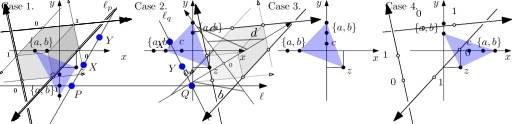
Figure 2: Left: The marked point associated with three skew lines in $\mathbb{R}^{3}$. Right: In $\mathbb{R}^{2}$, if two lines crossing at ⁰ intersect segments $\{a,b,c,d\}$ in the (extended) orders $(ab{{}^{\mathbf{0}}}cd,b{{}^{\mathbf{0}}}adc)$, then the sets $c$ and $d$ must cross.

Analogy with the planar case.

A similar observation was used in the plane (see e.g. [16]). Consider two lines in $\mathbb{R}^{2}$, crossing in ⁰, and a family of segments, where each segment has an endpoint on each line (see Figure 2-right). Every segment lies in a (closed) quadrant formed by the lines, and two segments intersect if and only if they lie in the same quadrant and appear in different orders when seen “from ⁰”. The quadrant containing a given segment is determined by the positions of that segment’s endpoints with respect to ⁰. As mentioned in the introduction, a simple case analysis then yields that $(1234,2143)$ has no geometric realization in the plane. (See [2, Figure 3.4] for another example of such case analysis.)

Changes between two and three dimensions.

In the plane, given two permutations and the position of the crossing point of the two lines, either all choices of positions yield pairwise disjoint segments, or none of them does. In $\mathbb{R}^{3}$, the polynomials describing whether two triangles are disjoint requires in some cases to compare pairs $\{x_{i},f(z_{j})\}$, $\{y_{i},f(x_{j})\}$ or $\{z_{i},f(y_{j})\}$ (Table 1). This makes it possible for two pairs of triangles, one crossing and the other disjoint, to realize the same three tagged permutations, i.e. have their vertices in the same position relative to the parallelotope of the lines.

Tagged permutations and patterns.

Formally, we define a tagged permutation as a permutation of $\{^{\mathbf{0}},^{\mathbf{1}},1,2,\ldots,n\}$ in which ⁰ precedes ¹. We call a triple of tagged permutations a tagged pattern. A canonical realization of a tagged pattern is a set of triangles, with vertices on $\ell_{x}$, $\ell_{y}$ and $\ell_{z}$, such that $\ell_{x}$ (resp. $\ell_{y}$, $\ell_{z}$) intersects the triangles in the first (resp. second, third) permutation and such that the tagged corners of the parallelotope appear in the right position on each line.

Our experiments will use two more notions. Two tagged patterns are equivalent for canonical realizability if one can be transformed into the other by (i) relabeling the symbols other than ⁰ and ¹ bijectively, and (ii) applying a circular permutation to the triple. A tagged pattern is minimally forbidden if it has no canonical realization, and deleting any symbol other than ⁰ and ¹ from the three tagged permutations produces a tagged pattern which has a canonical realization.

5 Algorithm

We now present an algorithm that takes a tagged pattern as input and decides if it admits a canonical realization. Our initial problem of testing the geometric realizability of a triple of permutations of size $n$ reduces to $8\binom{n+2}{2}^{3}$ instances of that problem.

5.1 Outline

Following Sections 2 and 3, we search for an order on $\{0,1,\mathbf{t}_{1},\mathbf{t}_{2},\ldots,\mathbf{t}_{9n}\}$ satisfying the conditions of Proposition 3.3 and the formula $\psi$ (which defines $S$). To save breath, we call such an order good. We say that triangles $i$ and $j$ are disjoint in a partial order $\mathcal{P}$ if for every $c\in\mathbb{R}^{3n}$ such that the order on $\Lambda(c)$ is a linear extension of $\mathcal{P}$, the triangles $i$ and $j$ of $\mathcal{T}(c)$ are disjoint.

Our algorithm gradually refines a set of partial orders on $\{0,1,\mathbf{t}_{1},\mathbf{t}_{2},\ldots,\mathbf{t}_{9n}\}$ with the constraint that, at any time, every good order is a linear extension of at least one of these partial orders. (Note that we do not need to make $\psi$ explicit.) Every partial order is refined until all or none of its extensions are good, so that we can report success or discard that partial order. Refinements are done in two ways:

• branching over an uncomparable pair, meaning duplicating the partial order and adding the comparison in one copy, and its reverse in the other copy,

• forcing a comparison when it is required for the formula $S$ to be satisfiable.

We keep our algorithm as simple as possible to facilitate the verification of the algorithm, the code in Appendix B, and the geometric results proven with their aid. This comes at the cost of some efficiency, but we discuss some possible improvements in Section 5.3.

5.2 Description

Our poset representation stores (i) for each lifted variable the interval $(\cdot,0)$, $(0,1)$ or $(1,\cdot)$ that contains it, and (ii) a directed graph over the variables contained in the interval $(1,\cdot)$. The graph has $3n$ vertices, by Lemma 3.1. To compare two variables, we first retrieve the intervals containing them. If they differ, we can return the comparison readily. If they agree, then up to composing by $f$ or $f^{(2)}$ we can assume that both variables are in $(1,\cdot)$ and we use the graph to reply. We ensure throughout that the graph is saturated, i.e. is its own transitive closure. In our implementation, initialization takes $O(n^{3})$ time, elements comparison takes $O(1)$ time, and edge addition to the graph takes $O(n^{2})$ time.

We start with the poset of the comparisons forced by the tagged pattern: all pairs $(x_{i},x_{j})$, $\left(f(x_{i}),f(x_{j})\right)$, …, $\left(f^{(2)}(z_{i}),f^{(2)}(z_{j})\right)$ as well as pairs separated by $0$ or $1$. We next collect in a set $U$ the comparisons missing to compute the vectors $v(i,j)$.

Lemma 5.1.

$U$ contains only pairs of the form $z_{k}-f(y_{k})$, $x_{k}-f(z_{k})$, or $y_{k}-f(x_{k})$.

Proof 5.2.

Every orientation predicate considered involves three points of the same index. Consider for instance $[X_{i},Y_{i},Z_{i},X_{j}]$. Following Table 1, this decomposes into $(x_{i}-x_{j})(y_{i}-1)(z_{i}-f(y_{i}))$ and only the sign of the last term may be undecided. Other cases are similar and show that $U$ can only contain terms the form $z_{k}-f(y_{k})$, $x_{k}-f(z_{k})$, or $y_{k}-f(x_{k})$.

Every pair in $U$ corresponds to two variables with same index, so $|U|\leq 3n$. If $U$ contains the three pairs with a given index, then two of the eight choices for these three comparisons are cyclic, and can thus be ignored. We thus have at most $6^{n}$ ways to decide the order of the undeterminate pairs of $U$; call them candidates. For each candidate, we make a separate copy of our current graph and perform the following operations on that copy:

1. We add the $|U|$ edges ordering the undecided pairs as fixed by the candidate and compute its transitive closure. We check that the result is acyclic; if not, we discard that candidate (as it makes contradictory choices) and move to the next candidate.

2. Let $\mathcal{P}$ denote the resulting partial order. We consider every $1\leq i<j\leq n$ in turn. (Note that $v(i,j)$ is determined and equal for all linear extensions of $\mathcal{P}$.)

   1. [2a]

   2. If $v(i,j)_{1}=v(i,j)_{2}=v(i,j)_{3}$ or $v(i,j)_{4}=v(i,j)_{5}=v(i,j)_{6}$ then triangles $i$ and $j$ are disjoint in $\mathcal{P}$. We move on to the next pair $(i,j)$.

   3. Otherwise, the extensions of $\mathcal{P}$ in which the triangles $i$ and $j$ are disjoint are those in which $[A_{i},B_{i},A_{j},B_{j}]=1$ or $[A_{i},C_{i},C_{j},A_{j}]=1$ (in the notations of Section 2). Lemma 5.3 asserts that $\mathcal{P}$ already determines at least one of these two predicates.

      1. [2b1]

      2. If both tests are determined to false, then triangles $i$ and $j$ intersect in $\mathcal{P}$. We then discard $\mathcal{P}$ and move on to the next candidate.

      3. If one test is determined to false and the other is undetermined, then that second test must evaluate to true in every good extension of $\mathcal{P}$. Again, by Table 1 we are missing exactly one comparison to decide that test. We add it to our graph.

      4. In the remaining cases, at least one test is determined to true, so triangles $i$ and $j$ are disjoint in $\mathcal{P}$. We move on to the next pair $(i,j)$.

3. If we exhaust all $(i,j)$ for a candidate, then we report “realizable”.

4. If we exhaust the candidates without reaching step $3$, then we report “unrealizable”.

This algorithm relies on property whose computer-aided proof is discussed in Section 6:

Lemma 5.3.

At step $2b$, at least one of $[A_{i},B_{i},A_{j},B_{j}]$ or $[A_{i},C_{i},C_{j},A_{j}]$ is determined.

5.3 Discussion

Let us make a few comments on our algorithm.

Correctness.

Let $\mathcal{P}_{0}$ denote the initial poset. First, remark that we explore the candidates exhaustively, so every good extension of $\mathcal{P}_{0}$ is a good extension of $\mathcal{P}_{0}$ augmented by (at least) one of the candidates. Next, consider the poset $\mathcal{P}$ obtained in step 2. When processing a pair $(i,j)$, we either discard $\mathcal{P}$ if we detect that $i$ and $j$ intersects in it (2b1) or we move on to the next pair $(i,j)$ after having checked (2a, 2b3) or ensured (2b2) that triangles $i$ and $j$ are disjoint in $\mathcal{P}$. If we reach step 3, then all extensions of the current partial order are good and we correctly report feasibility. If a candidate is discarded then no linear extension of $\mathcal{P}$ augmented by that candidate is a good order. If we reach Step 4, then every candidate has been discarded, so no linear extension of $\mathcal{P}_{0}$ was a good order to begin with, and we correctly report unfeasibility.

Complexity.

Initializing the poset and computing $U$ take $O(n^{3})$ time. We have at most $6^{n}$ candidates to consider. Step 1 takes $O(n^{3})$ time. The steps 2a-2b3 are executed $O\left(n^{2}\right)$ times, and the bottleneck among them is 2b2, which takes $O(n^{2})$ time. Altogether, our algorithm decides if a tagged pattern is realizable in $O\left(6^{n}n^{4}\right)$ time.

Improvements.

In practice, the algorithm we presented can be sped up in several ways. For example, it is much better to branch over the pairs of $U$ one by one. Once a branching is done, we can update $U$ by removing the pairs that have become comparable, and thus avoid examining candidates that would get discarded at Step 1. Also, it pays off to record the forbidden tagged patterns of small size, and, given a larger tagged pattern to test, check first that it does not contain a small forbidden pattern.

One-sided certificate.

If the algorithm reaches Step 3, we actually know a poset for which every linear extension is good. This means that we can compute an arbitrary linear extension to obtain an order on the variables in $(1,\cdot)$. We can then assign to these variables any values that satisfy this order, say by choosing the integers from $2$ to $3n+1$, and then propagate these values via $f$ and $f^{(2)}$ to all lifted variables. From there, we can extract the values of $x_{1},x_{2},\ldots,z_{n}$ of a concrete realization of our tagged pattern. In this way, all computations are done on (relatively small) rationals and are therefore easy to do exactly.

6 Experimental results

We now discuss our implementation of the above algorithm as well as its experimental use. Remember that we call a tagged pattern forbidden if it admits no canonical realization. We make the raw data available (see Appendix A).

Implementation.

We implemented the algorithm of Section 5 in Python 3, and comment on its key functions in Appendix B. For simplicity, our implementation makes one adjustment to the algorithm: we branch over all $2^{|U|}$ choices for the pairs of undecided variables; so, we take $8$ choice per $k$, rather than $6$. Altogether, the implementation amounts to $\sim 470$ lines of (commented) code and is sufficiently effective for our experiments: on a standard desktop computer, finding all realizable triples of size $6$ (and a realization when it exists) takes about $40$ minutes, whereas verifying that no minimally forbidden tagged pattern of size $6$ exists took up about a month of computer time; the difference of course is that in the former, for realizable triples we do not have to look at all positions of tags.

Proof of Lemma 5.3.

The statement concerns only two triangles and can be shown by a simple case analysis. Our code sets up an exception that is raised if the statement of the lemma fails (cf line 94 in the code in Appendix B.1). Checking the realizability of all tagged patterns on two elements exhausts the case analysis, and the exception is not raised.

Minimally forbidden patterns.

To state the minimally forbidden tagged patterns of size $3$ we compress the notation as follows. We use $\{uv\}$ to mean “$uv$ or $vu$”. Symbols that are omitted may be placed anywhere (this may include ⁰ and ¹). We use $x_{i}=y_{j}$ to mean “any pattern in which the $i$th symbol on the $1$st tagged permutation equals the $j$th symbol of the $2$nd tagged permutation”.

Proposition 6.1.

The equivalence classes of minimally forbidden tagged patterns are:

1. [(i)]

2. For size $2$, $(ab^{\mathbf{0}},^{\mathbf{1}}ab,ab)$, $(^{\mathbf{0}}ab,ab^{\mathbf{1}},ba)$, $(ab^{\mathbf{0}},ba^{\mathbf{1}},ab)$, and $(^{\mathbf{0}}ab,^{\mathbf{1}}ba,ba)$.

3. For size $3$, $(\{ab\}^{\mathbf{0}},\{ab\}c^{\mathbf{0}},z_{2}=y_{1})$, $(\{ab\}c^{\mathbf{0}},^{\mathbf{1}}\{ab\},z_{2}=x_{1})$, $(\{ab\}^{\mathbf{0}},^{\mathbf{1}}c\{ab\},z_{2}=y_{3})$, $(^{\mathbf{1}}c\{ab\},^{\mathbf{1}}\{ab\},z_{2}=x_{3})$, $(abc^{\mathbf{0}},b^{\mathbf{1}}ac,ca^{\mathbf{0}}b)$, and $(^{\mathbf{1}}abc,b^{\mathbf{1}}ca,ac^{\mathbf{0}}b)$.

4. For size $4$, the taggings of $(abcd,badc,cdab)$ that contains $(^{\mathbf{0}}b^{\mathbf{1}},^{\mathbf{1}}d,a^{\mathbf{0}})$ or $(b^{\mathbf{0}}c,^{\mathbf{1}}a,a^{\mathbf{0}})$, and the taggings of $(abcd,badc,dcba)$ that contains $(b^{\mathbf{0}}c,^{\mathbf{0}}d^{\mathbf{1}},^{\mathbf{1}}c)$ or $(c^{\mathbf{0}},\{^{\mathbf{0}}ba\}\{^{\mathbf{1}}dc\},^{\mathbf{1}}c)$.

5. None for size $5$ and $6$.

Realization database.

For every tagged pattern that our algorithm declared realizable, we computed a realization (as explained in Section 5.3) and checked it independently.

Geometric permutations.

It remains to prove our statements on geometric permutations:

Proof 6.2 (Proof of Theorem 1.1).

For every triple of permutations, we checked that it is realizable by trying all $8$ reversals and all $\binom 72^{3}$ possible positions of ⁰ and ¹, until we find a choice that does not contain any minimally forbidden tagged pattern of Proposition 6.1.

Proof 6.3 (Proof of Theorem 1.2).

We argue by contradiction. Consider four disjoint convex sets met by lines $\ell_{1}$, $\ell_{2}$ in the order $abcd$ and $\ell_{3}$ in the order $badc$; assume that $\ell_{1}\odot\ell_{3}=-\ell_{2}\odot\ell_{3}$. By the perturbation argument of Lemma 2.1, we can assume that the three lines are pairwise skew and that the convex sets are triangles with vertices on these lines. Moreover, there exists a nonsingular affine transform $A$ that maps the unoriented lines $\ell_{1}$ to $\ell_{x}$, $\ell_{2}$ to $\ell_{y}$ and $\ell_{3}$ to $\ell_{z}$. Remark that $A$ either preserves or reverses all side operators. Since $\ell_{x}\odot\ell_{z}=\ell_{y}\odot\ell_{z}$ and $\ell_{1}\odot\ell_{3}=-\ell_{2}\odot\ell_{3}$, the map $A$ sends the oriented lines $(\ell_{1},\ell_{2})$ to either $(\ell_{x},-\ell_{y})$ or $(-\ell_{x},\ell_{y})$. We used our program to check that none of $(abcd,dcba,badc)$, $(dcba,abcd,badc)$, $(abcd,dcba,cdab)$, $(dcba,abcd,cdab)$ admits a canonical realization. The statement follows.

7 Geometric analysis

We present here an independent proof that the tagged patterns of size $2$ and $3$ listed in Proposition 6.1 do not have a (canonical) realization. We do not prove the patterns are minimal, nor do we prove that the list is exhaustive; these facts come from the completeness of our computer-aided enumeration.

7.1 Size two

The following observation was used by Asinowski and Katchalski [3]:

Observation 7.1.

Let $X$ and $Y$ be compact convex sets and let $P$ and $Q$ be points in $\mathbb{R}^{3}$. Assume that $X,Y,P,Q$ are pairwise disjoint and that there exist lines inducing the geometric permutation $(PXY)$ and $(QYX)$. Any oriented line with direction $\overrightarrow{PQ}$ that intersects $X$ and $Y$, must intersect $X$ before $Y$.

Proof 7.2.

Refer to the figure. Let $h$ be a plane that separates $X$ and $Y$. The existence of the geometric permutations $(PXY)$ and $(QYX)$ ensure that $h$ also separates $P$ and $Q$. Moreover, the halfspace bounded by $h$ that contains $X$ also contains $P$, so any line with direction $\overrightarrow{PQ}$ traverses $h$ from the side of $X$ to the side of $Y$.

Observation 7.1 implies that $(ab^{\mathbf{0}},^{\mathbf{1}}ab,ab)$, $(^{\mathbf{0}}ab,ab^{\mathbf{1}},ba)$, $(ab^{\mathbf{0}},ba^{\mathbf{1}},ab)$, and $(^{\mathbf{0}}ab,^{\mathbf{1}}ba,ba),$ are forbidden. Indeed, consider, by contradiction, a realization of one of these tagged patterns. Let $P$ be the point ⁰ on $\ell_{x}$ and $Q$ the point ¹ on $\ell_{y}$. In each case, we can map $X$ and $Y$ to $a$ and $b$ so that some line $\ell_{P}\in\{\ell_{x},-\ell_{x}\}$ realizes $PXY$ and $\ell_{Q}\in\{\ell_{y},-\ell_{y}\}$ realizes $QYX$. Then, Observation 7.1 implies that any line with same direction as the line from $P$ to $Q$ must intersect $X$ before $Y$; this applies to the line $\ell_{z}$ and contradicts the fact that the configuration realizes the chosen tagged pattern.

7.2 Size three

To argue that the tagged patterns of size $3$ of Proposition 6.1 are forbidden we first need a basic observation concerning planar geometric permutations.

Observation 7.3.

Suppose the $x$-axis and the $y$-axis are transversal to three disjoint convex sets in $\mathbb{R}^{2}$. Suppose furthermore that all the sets intersect the $x$-axis in points $x_{1},x_{2},x_{3}$, where either $x_{1}<x_{2}<x_{3}\leq 0$ or $0\leq x_{1}<x_{2}<x_{3}$. Then the middle element of the geometric permutation induced by the $y$-axis can not equal the extreme element of the $x$-axis. (Here the extreme element refers to the set intersected the farthest away from the origin on the $x$-axis.)

Proof 7.4.

Lets call the sets $A_{1}$, $A_{2}$, $A_{3}$. Up to symmetry we may assume that the sets intersect the $x$-axis in the points $0\leq x_{1}<x_{2}<x_{3}$ where $x_{i}\in A_{i}$. This means that $A_{3}$ is the extreme element of the $x$-axis. Now suppose for contradiction that $A_{3}$ is the middle element of the geometric permutation determined by the $y$-axis, so the $y$-axis meets the sets in points $y_{i}<y_{3}<y_{j}$, with $y_{k}\in A_{k}$. If $0<y_{3}$, then the segment $[x_{j},y_{j}]$ intersects the segment $[x_{3},y_{3}]$, and if $y_{3}<0$, then the segment $[x_{i},y_{i}]$ intersects the segment $[x_{3},y_{3}]$.

Now, Proposition 6.1 (ii) asserts that the patterns

$$\begin{array}[]{ll}1.\quad(\{ab\}^{\mathbf{0}},\{ab\}c^{\mathbf{0}},z_{2}=y_{1}),&4.\quad(^{\mathbf{1}}c\{ab\},^{\mathbf{1}}\{ab\},z_{2}=x_{3}),\\ 2.\quad(\{ab\}c^{\mathbf{0}},^{\mathbf{1}}\{ab\},z_{2}=x_{1}),&5.\quad(abc^{\mathbf{0}},b^{\mathbf{1}}ac,ca^{\mathbf{0}}b),\\ 3.\quad(\{ab\}^{\mathbf{0}},^{\mathbf{1}}c\{ab\},z_{2}=y_{3}),&6.\quad(^{\mathbf{1}}abc,b^{\mathbf{1}}ca,ac^{\mathbf{0}}b).\end{array}$$

are forbidden. The basic idea of the proof of this fact is to show under the given conditions we can find another transversal line that intersects one of the lines $\ell_{x}$, $\ell_{y}$, $\ell_{z}$ to obtain a pair of crossing lines where we can apply Observation 7.3.

For patterns 1–4, the line we are looking for is just a translate of the line $\ell_{z}$. The translation can be found by considering an appropriate projection. In Figure 3 we see projections of patterns 1–4 to the $xy$-plane.

Figure 3: Projections to the $xy$-plane of the patterns 1–4. In each case the projection of triangles $a$ and $b$ contain the point labeled by $c$.

Specifically:

• In cases 1 and 3 we see that the line $\ell^{\prime}$ parallel to $\ell_{z}$ which passes through the point $c_{y}$ (the point of $c$ on the line $\ell_{y}$) is transversal to all the sets. Therefore we can apply Observation 7.3 with $\ell_{y}$ as the $x$-axis and $\ell^{\prime}$ as the $y$-axis.

• In cases 2 and 4 we see that the line $\ell^{\prime}$ parallel to $\ell_{z}$ which passes through the point $c_{x}$ is transversal to all the sets. Therefore we can apply Observation 7.3 with $\ell_{x}$ as the $x$-axis and $\ell^{\prime}$ as the $y$-axis.

For cases 5 and 6 we will need one additional observation:

Observation 7.5.

Consider two lines $\ell_{1}$ and $\ell_{2}$ in $\mathbb{R}^{3}$ and three segments $a$, $b$ and $c$, each with one endpoint on $\ell_{1}$ and one endpoint on $\ell_{2}$. Assume that $a$, $b$ and $c$ are pairwise non-coplanar and not all three parallel to a common plane. Put $a_{i}=a\cap\ell_{i}$ and parameterize the segment $a_{1}a_{2}$ as $a(t)=(1-t)a_{1}+ta_{2}$, $t\in[0,1]$. Let $\ell(t)$ denote the line through $a(t)$ that intersects or is parallel to the lines supporting respectively $b$ and $c$. The lines $\ell_{1}$ and $\ell_{2}$ realize the same geometric permutation of $\{a,b,c\}$ if and only if for every $t\in[0,1]$ the line $\ell(t)$ intersects the three segments $a$, $b$ and $c$.

Proof 7.6.

Let us first reformulate the statement. For $s\in\{a,b,c\}$ let $\ell_{s}$ denote the line supporting $s$. The intersection point $\ell(t)\cap\ell_{b}$ moves along $\ell_{b}$ from $\ell_{1}\cap\ell_{b}$ to $\ell_{2}\cap\ell_{b}$ by travelling either along the segment $b$, or along $\ell_{b}\setminus b$. We are in the latter case if and only if for some $0<t<1$ the line $\ell(t)$ is parallel to $\ell_{b}$. The same holds for $c$. The statement therefore reformulates as: $\ell_{1}$ and $\ell_{2}$ realize the same geometric permutation of $\{a,b,c\}$ if and only if no line $\ell(t)$ is parallel to $\ell_{b}$ or $\ell_{c}$. Now, the reformulated statement follows from elementary considerations on the geometry of ruled quadric surfaces (see for instance the projective geometry textbook of Veblen and Young [28, Chapter 11]). Let us spell it out.

Since $\ell_{a}$, $\ell_{b}$ and $\ell_{c}$ are in general position, these lines and all their common transversals are contained in a quadric surface $H$, specifically a hyperbolic paraboloid. The quadric $H$ has two families of rulings, one which contains $\{\ell_{a},\ell_{b},\ell_{c}\}$ and the other that we denote as $R$. Every line in one family of rulings intersects or is parallel to every line in the other family of rulings.

Consider a space parameterizing the lines of $\mathbb{R}^{3}$ bicontinuously (for instance via Plücker coordinates) and identify a line with its parameter point. In that space, $R$ forms a closed loop and it contains five points of interest to us: $\ell_{1}$ and $\ell_{2}$, as well as three special lines, which are transversals to two of $\{\ell_{a},\ell_{b},\ell_{c}\}$ and parallel to the third one. Let us denote the special lines by $\ell_{a}^{*}$, $\ell_{b}^{*}$ and $\ell_{c}^{*}$, where $\ell_{s}^{*}$ is parallel to $\ell_{s}$.

The special lines $\ell_{a}^{*}$, $\ell_{b}^{*}$ and $\ell_{c}^{*}$ therefore split $R$ into three open arcs, and two line transversals to $\{\ell_{a},\ell_{b},\ell_{c}\}$ realize the same (untagged) geometric permutation if and only if these lines belong to the same arc. Indeed, as a line $\ell$ moves continuously on $R$, its intersection points with $\ell_{a}$, $\ell_{b}$ and $\ell_{c}$ change continuously – and in particular the order in which the line meets $\ell_{a}$, $\ell_{b}$ and $\ell_{c}$ remains unchanged – except as the $\ell$ reaches one of the special line $\ell_{s}^{*}$: when that happens, the intersection with $\ell_{s}$ jumps from one “end” of $\ell$ to its other “end”. Formally, as $\ell$ passes one of $\ell_{a}^{*}$, $\ell_{b}^{*}$ and $\ell_{c}^{*}$, the order in which the moving line intersects $\ell_{a}$, $\ell_{b}$ and $\ell_{c}$ changes by a circular permutation.

Now consider the set of lines $\gamma=\{\ell(t)\colon 0\leq t\leq 1\}$. This is an arc contained in $R$, bounded by $\ell_{1}$ and $\ell_{2}$ and, by assumption, not containing $\ell_{a}^{*}$. It follows that $\ell_{1}$ and $\ell_{2}$ realize the same geometric permutation of $\{a,b,c\}$ if and only if $\gamma$ contains neither $\ell_{b}^{*}$ nor $\ell_{c}^{*}$. This is precisely the reformulation of the statement.

Let us now get back to proving that the tagged patterns 5 and 6 are forbidden. Notice that in both cases, the directed lines $\ell_{y}$ and $-\ell_{z}$ induce the same permutations. Thus, by Observation 7.5 there is a continuous family of directed lines $\{\ell(t):0\leq t\leq 1\}$ that are all transversal to the segments $a$, $b$ and $c$ in the same order; moreover, $\ell(0)=\ell_{y}$ and $\ell(1)=-\ell_{z}$. Next notice that $\ell_{y}$ and $-\ell_{z}$ lie on opposite sides of the line $\ell_{x}$ (that is, $\ell_{y}\odot\ell_{x}\neq(-\ell_{z})\odot\ell_{x}$), so by continuity there exists $0<t^{\prime}<1$ such that the directed line $\ell^{\prime}=\ell(t^{\prime})$ intersects the line $\ell_{x}$. We now apply Observation 7.3 to the pair of lines $\ell_{x}$ and $\ell^{\prime}$.

We start with Case 5. The line $\ell^{\prime}$ intersects the segments in the order $b\prec a\prec c$, and we will consider where the intersection point $P=\ell_{x}\cap\ell^{\prime}$ fits into this ordering. If the order of intersection along $\ell^{\prime}$ is $b\prec a\prec c\prec P$, then we can apply Observation 7.3 with $\ell^{\prime}$ as the $x$-axis and $\ell_{x}$ as the $y$-axis. We may therefore assume that $P\prec c$. If we in addition have $b\prec P$, then it follows that the $x$-coordinate of $P$ is non-negative. To see this observe that the $x$-coordinates of the points on segments $[b_{y},b_{z}]$ and $[c_{y},c_{z}]$ are between $0$ and $1$, so the same holds for any point on the line $\ell^{\prime}$ which is between $b$ and $c$, in particular for the point $P$. Since the points $a_{x},b_{x},c_{x}$ all have negative $x$-coordinates it follows that the line $\ell_{x}$ intersects the points in the order $a\prec b\prec c\prec P$, and we may therefore apply Observation 7.3 with $\ell_{x}$ as the $x$-axis and $\ell^{\prime}$ as the $y$-axis. The final situation to be considered is if $\ell^{\prime}$ intersects the points in the order $P\prec b\prec a\prec c$. However the plane $\{y+z=1\}$ strictly separates the segment $[b_{y},b_{z}]$ from $[a_{y},a_{z}]\cup[c_{y},c_{z}]\cup\ell_{x}$, and so if the order along $\ell^{\prime}$ was $P\prec b\prec a\prec c$, this would force $\ell^{\prime}$ to intersect the plane $\{y=z+1\}$ twice, a contradiction.

Now for Case 6 which is similar. The line $\ell^{\prime}$ intersects the segments in the order $b\prec c\prec a$ and we want to place the intersection point $P=\ell_{x}\cap\ell^{\prime}$ in this ordering. If we have $b\prec c\prec a\prec P$ then we can apply Observation 7.3 with $\ell^{\prime}$ as the $x$-axis and $\ell_{x}$ as the $y$-axis. If we have $b\prec P\prec a$, then the $x$-coordinate of the point $P$ is at most $1$ (since the $x$-coordinates of the points on the segments $[b_{y},b_{z}]$ and $[a_{y},a_{z}]$ are between $0$ and $1$). We may therefore apply Observation 7.3 with $\ell_{x}$ as the $x$-axis and $\ell^{\prime}$ as the $y$-axis. The final situation is the order $P\prec b\prec c\prec a$ which is impossible since the plane $\{y+z=1\}$ separates the segment $[b_{y},b_{z}]$ from $[a_{y},a_{z}]\cup[c_{y},c_{z}]\cup\ell_{x}$.

Appendix A Additional material

We provide the following additional material:

• The python code. See the README.txt file for how to invoke it.

• Some output files summarizing the results of our experiments:

  • The list of triples of permutations of size five with, for each, the coordinates of a geometric realization. The triples are normalized in the sense defined in Appendix LABEL:a:forbid6.

  • The list of triples of size six with, for each, either the coordinates of a geometric realization or the statement that none exists.

We make this material available from

https://hal.inria.fr/hal-02050539/file/Code.tar.gz.

Appendix B Code

We present here the implementation that we used for our experiments. We do not reproduce the entire code as it is not so informative, but explain how its key functions operate. Readers interested in the full code can get it from the url given in Appendix A.

B.1 compute_realization_tagged

The function compute_realization_tagged is the main algorithm. It checks whether a given triplet of tagged permutations is canonically realizable, and output a realization if the answer is positive.

Encoding.

Permutations of $\{0,\ldots,n-1\}$ are encoded as lists. Tagged are encoded separately as pairs $[z,o]$ where $z$ (resp. $o$) is the position of the zero (resp. of the one), defined as the number of elements smaller than zero (resp. one). For instance $23|^{\bf 0}0|^{\bf 1}1$ is encoded with the permutation $[2,3,0,1]$ and the tags $[2,3]$.

Our algorithm first consists of collecting the information that is missing to compute the sign vectors of Guigue-Devillers’ algorithm in a set $U$. As stated in Lemma 5.1, it only contains specific pairs, such as $x_{k}-f(z_{k})$, which are encoded by the number associated with $x_{k}$. The numbers of $x_{i}$, $y_{j}$ and $z_{k}$ are $i$, $n+j$ and $2n+k$, respectively.

In $M$ we keep the transitive closure of the adjacency matrix of the graph that collects the orientations induced by the tagged permutations and by the current orientations of the elements in $U$. This graph represents the poset of the relative orders of the variables greater than one: if $x_{2}$ is between $0$ and $1$, the associated vertex number $2$ represents $f(x_{2})$ and if $y_{1}$ is smaller than $0$, the associated vertex $n+1$ represents $f^{2}(y_{1})$.

Auxiliary functions.

The function compute_realization_tagged uses the following simple algorithms, for which we do not give the code here:

• associated_vertex(v) is the only variable $w$ such that $v-f(w)$ can appear in $U$.

• compute_base_graph build the adjacency matrix of the graph with an edge $v\rightarrow w$ whenever $v$ and $w$ are on the same line, in the same interval, and $v$ is before $w$ in the associated permutation.

• transitive_acyclic(M) add an edge $v\rightarrow w$ whenever there is a non-trivial path from $v$ to $w$, using Warshall algorithm. Halts and return false if $M$ is not acyclic.

• add_edge_closure(M,v,w) add an edge $v\rightarrow w$ and update the transitive closure.

• topological_sort(M) compute an ordering of the vertices compatible with the graph, using the classical depth-first algorithm.

Code of the function.

[language=Python] def compute_realization_tagged(perm_triplet, tag_triplet): Px, Py, Pz = perm_triplet n = len(Px) Ix, Iy, Iz = inverse_perm(Px), inverse_perm(Py), inverse_perm(Pz) inv_triplet = [Ix, Iy, Iz]

# precompute the interval of each vertex: # 0 if ¡0, 1 if between 0 & 1, and 2 if ¿1 regions = [compute_region(v, inv_triplet, tag_triplet) for v in range(3*n)]

# initialization of the adjacency matrix of the graph M = [[False]*(3*n) for _in range(3*n)]

# the base matrix containing information from the perms and tags B = compute_base_graph(perm_triplet, tag_triplet)

# SV is a map, s.t. SV[(i,j)] is the sign vector of (i,j), # which is a 6-tuple containing pairs of the form (sign, unknown): # sign = +- 1 and unknown = None if the sign is determined; # otherwise, unknown = v if the value is the sign of sign*(v-f(w)) # U is the set of unknown and required v-f(w), # identified by their v (w is associated_vertex(v)) SV, U = , set([]) for i, j in combinations(range(n), 2): SV[(i, j)] = list() for l in range(3): SV[(i, j)].append(compute_initial_orientation(i, l, j, inv_triplet, regions, U)) for l in range(3): SV[(i, j)].append(compute_initial_orientation(j, l, i, inv_triplet, regions, U)) m = len(U)

# main loop: iteration over the orientations of the elements of U for it in range(2**m): # copy the base B into M for ii, jj in product(range(3*n),range(3*n)): M[ii][jj] = B[ii][jj] # if the i-th bit of ”it” is 1 then v ¡ f(w) for the i-th v # of U and v ¿ f(w) otherwise j = it for v in U: w = associated_vertex(v, n) if j M[v][w] = True else: M[w][v] = True j //= 2 # continue the bit decomposition if not transitive_acyclic(M): # the graph is not acyclic, we try the next choice of # orientations for the elements in U continue for i, j in combinations(range(n), 2): # check whether they are pairwise disjoint intersection = False # used to halt the loop if needed # compute the sign vector of (i,j), now that # we have all the required information stored in M sv = compute_sign_vector(SV[(i, j)], M)

# we now apply the Devillers-Guigue algorithm if sv[0] == sv[1] == sv[2] or sv[3] == sv[4] == sv[5]: # the two triangles are disjoint, go to the next pair continue # compute the numbers associated with the variables Xi, Yi, Zi, Xj, Yj, Zj = i, i+n, i+2*n, j, j+n, j+2*n # order the points as in the Devillers-Guigue’s algorithm sign_i, sign_j = sv[0], sv[3] if sv[0] == sv[1]: Xj, Yj, Zj = Zj, Xj, Yj sign_i = sv[2] elif sv[0] == sv[2]: Xj, Yj, Zj = Yj, Zj, Xj sign_i = sv[1] if sv[3] == sv[4]: Xi, Yi, Zi = Zi, Xi, Yi sign_j = sv[5] elif sv[3] == sv[5]: Xi, Yi, Zi = Yi, Zi, Xi sign_j = sv[4] if sign_i == -1: Yi, Zi = Zi, Yi if sign_j == -1: Yj, Zj = Zj, Yj # the points have been permuted so that their sign vector # is now (1,-1,-1,1,-1,-1). We (try to) compute the two # orientations of the algorithm: # each O is either sign, None if determined # or sign, [v,w] if it has the sign of sign*(v-f(w)) O1 = compute_last([Xi,Yi,Xj,Yj], M, inv_triplet, regions) O2 = compute_last([Xi,Zi,Zj,Xj], M, inv_triplet, regions) if O1[1] is not None and O2[1] is not None: # for some reason, this case never happen raise Exception(”Both orientations are unknown”) if O1[1] is None and O1[0] == 1: continue # the two triangles are disjoint if O2[1] is None and O2[0] == 1: continue # the two triangles are disjoint if O1[1] is None and O2[1] is None: # they are both -1 at this point =¿ intersection intersection = True break # the (i,j) loop if O1[1] is None: # O1 is -1 and O2 is unknown: it has to be 1 v, w = O2[1] if O2[0] == 1: add_edge_closure(M, w, v) # v - f(w) ¿ 0 else: add_edge_closure(M, v, w) # v - f(w) ¡ 0 if O2[1] is None: # O2 is -1 and O1 is unknown: it has to be 1 v, w = O1[1] if O1[0] == 1: add_edge

References

- [1] B Aronov and S. Smorodinsky. On geometric permutations induced by lines transversal through a fixed point. Discrete & Computational Geometry, 34:285–294, 2005.
- [2] Andrei Asinowski. Geometric permutations for planar families of disjoint translates of a convex set. Technion-Israel Institute of Technology, Faculty of Mathematics, 1999.
- [3] Andrei Asinowski and Meir Katchalski. Forbidden Families of Geometric Permutations in . Discrete & Computational Geometry, 34(1):1–10, 2005. URL: \urlhttp://dx.doi.org/10.1007/s00454-004-1110-x.
- [4] O. Cheong, X. Goaoc, and H.-S. Na. Geometric permutations of disjoint unit spheres. Computational Geometry: Theory & Applications, 30:253–270, 2005.
- [5] Felipe Cucker, Peter Bürgisser, and Pierre Lairez. Computing the homology of basic semialgebraic sets in weak exponential time. arXiv preprint arXiv:1706.07473, 2017.
- [6] James H Davenport and Joos Heintz. Real quantifier elimination is doubly exponential. Journal of Symbolic Computation, 5(1-2):29–35, 1988.
- [7] Herbert Edelsbrunner and Micha Sharir. The maximum number of ways to stab convex non-intersecting sets in the plane is . Discrete & Computational Geometry, 5:35–42, 1990.
- [8] B. Grünbaum. On common transversals. Archiv der Mathematik, 9:465–469, 1958.
- [9] Philippe Guigue and Olivier Devillers. Fast and robust triangle-triangle overlap test using orientation predicates. Journal of graphics tools, 8(1):25–32, 2003.
- [10] Jae-Soon Ha, Otfried Cheong, Xavier Goaoc, and Jungwoo Yang. Geometric permutations of non-overlapping unit balls revisited. Computational Geometry, 53:36–50, 2016.
- [11] Andreas Holmsen and Rephael Wenger. Helly-type Theorems and geometric transversals. Handbook of discrete and computational geometry, CRC Press Ser. Discrete Math. Appl, pages 63–82, 2017.
- [12] Erich Kaltofen, Bin Li, Zhengfeng Yang, and Lihong Zhi. Exact certification in global polynomial optimization via sums-of-squares of rational functions with rational coefficients. J. Symb. Comput., 47(1):1–15, 2012.
- [13] M Katchalski. A conjecture of Grünbaum on common transversals. Math. Scand., 59:192–198, 1986.
- [14] M. Katchalski, T. Lewis, and J. Zaks. Geometric permutations for convex sets. Discrete Math., 54:271–284, 1985.
- [15] M Katchalski, Ted Lewis, and A Liu. Geometric permutations and common transversals. Discrete & Computational Geometry, 1(4):371–377, 1986.
- [16] Meir Katchalski, Ted Lewis, and Joseph Zaks. Geometric permutations for convex sets. Discrete mathematics, 54(3):271–284, 1985.
- [17] Jan Kratochvíl and Jirí Matousek. Intersection graphs of segments. J. Comb. Theory, Ser. B, 62(2):289–315, 1994.
- [18] Henri Lombardi, Daniel Perrucci, and Marie-Françoise Roy. An elementary recursive bound for effective Positivstellensatz and Hilbert 17-th problem. arXiv preprint arXiv:1404.2338, 2014.
- [19] A. Marcus and G. Tardos. Excluded permutation matrices and the Stanley–Wilf conjecture. J. Combin. Theory Ser. A, 107:153–160, 2004.
- [20] János Pach and Micha Sharir. Combinatorial geometry and its algorithmic applications: The Alcalá lectures. 152. American Mathematical Soc., 2009.
- [21] James Renegar. On the computational complexity and geometry of the first-order theory of the reals. Part I: Introduction. Preliminaries. The geometry of semi-algebraic sets. The decision problem for the existential theory of the reals. Journal of symbolic computation, 13(3):255–299, 1992.
- [22] Natan Rubin, Haim Kaplan, and Micha Sharir. Improved bounds for geometric permutations. SIAM Journal on Computing, 41(2):367–390, 2012.
- [23] Marcus Schaefer and Daniel Štefankovič. Fixed points, Nash equilibria, and the existential theory of the reals. Theory of Computing Systems, 60(2):172–193, 2017.
- [24] S. Smorodinsky, J.S.B Mitchell, and M. Sharir. Sharp bounds on geometric permutations for pairwise disjoint balls in . Discrete & Computational Geometry, 23:247–259, 2000.
- [25] Csaba D Toth, Joseph O’Rourke, and Jacob E Goodman. Handbook of discrete and computational geometry. Chapman and Hall/CRC, 2017.
- [26] H. Tverberg. Proof of Grünbaum’s conjecture on common transversals for translates. Discrete & Computational Geometry, 4:191–203, 1989.
- [27] Helge Tverberg. On geometric permutations and the Katchalski-Lewis conjecture on partial transversals for translates. DIMACS Ser. Discrete Math. Theor. Comp. Sci., 6:351–361, 1991.
- [28] Oswald Veblen and John W. Young. Projective Geometry, volume 1. Blaisdell Publishing Co., 1910.