Accelerated convergence to equilibrium and reduced asymptotic variance for Langevin dynamics using Stratonovich perturbations

Résumé

In this paper we propose a new approach for sampling from probability measures in, possibly, high dimensional spaces. By perturbing the standard overdamped Langevin dynamics by a suitable Stratonovich perturbation that preserves the invariant measure of the original system, we show that accelerated convergence to equilibrium and reduced asymptotic variance can be achieved, leading, thus, to a computationally advantageous sampling algorithm. The new perturbed Langevin dynamics is reversible with respect to the target probability measure and, consequently, does not suffer from the drawbacks of the nonreversible Langevin samplers that were introduced in [C.-R. Hwang, S.-Y. Hwang-Ma, and S.-J. Sheu, Ann. Appl. Probab. 1993] and studied in, e.g. [T. Lelievre, F. Nier, and G. A. Pavliotis J. Stat. Phys., 2013] and [A. B. Duncan, T. Lelièvre, and G. A. Pavliotis J. Stat. Phys., 2016], while retaining all of their advantages in terms of accelerated convergence and reduced asymptotic variance. In particular, the reversibility of the dynamics ensures that there is no oscillatory transient behaviour. The improved performance of the proposed methodology, in comparison to the standard overdamped Langevin dynamics and its nonreversible perturbation, is illustrated on an example of sampling from a two-dimensional warped Gaussian target distribution.

Résumé Convergence accélérée vers l’équilibre et variance asymptotique réduite pour la dynamique de Langevin à l’aide de perturbations de Stratonovich. Dans cet article, nous proposons une nouvelle approche pour l’échantillonnage de mesures invariantes dans des espaces de grandes dimensions à l’aide d’une dynamique de Langevin perturbée. En modifiant la dynamique standard de l’équation de Langevin suramortie en introduisant une perturbation de Stratonovich convenable préservant la mesure invariante du système initial, nous montrons qu’il est possible d’obtenir une convergence accélérée vers l’équilibre et une variance asymptotique réduite, conduisant ainsi à un algorithme d’échantillonnage avantageux du point de vue du calcul. La nouvelle dynamique de Langevin perturbée est réversible par rapport à la mesure de probabilité cherchée et ne souffre donc pas des inconvénients des échantillonneurs de Langevin non réversibles introduits dans [C.-R. Hwang, S.-Y. Hwang-Ma, and S.-J. Sheu, Ann. Appl. Probab. 1993] et étudiés par exemple dans [T. Lelievre, F. Nier, and G. A. Pavliotis J. Stat. Phys., 2013] et [A. B. Duncan, T. Lelièvre, and G. A. Pavliotis J. Stat. Phys., 2016], tout en conservant tous leurs avantages en termes de convergence accélérée et de réduction de la variance asymptotique. En particulier, la réversibilité de la dynamique garantit l’absence de comportement transitoire oscillant. Les performances améliorées de la méthodologie proposée, par rapport à la dynamique de Langevin suramortie standard et à sa perturbation irréversible, sont illustrées par un exemple d’échantillonnage à partir d’une distribution gaussiennes déformées à deux dimensions.

, ,

1 Introduction

Sampling from probability measures in high dimensional spaces is an important problem that arises in several applications, including computational statistical physics [8], Bayesian inference [13], and machine learning [1]. Typically one is interested in calculating integrals of the form

$$\pi(\phi):={\mathbb{E}}_{\pi}\phi:=\int_{\mathbb{R}^{d}}\phi(x)\,\pi(dx),$$ (1)

where $\pi(dx)=\pi(x)\,dx$ is a probability measure in $\mathbb{R}^{d}$, known up to the normalization constant and $\phi\in L^{2}(\pi)$ is an observable. Here $L^{2}(\pi)$ denotes the weighted $L^{2}$ space for the scalar product $(\phi,\psi)_{\pi}=\int_{\mathbb{R}^{d}}\phi(x)\psi(x)\pi(x)dx$ and the corresponding norm is denoted by $\|\phi\|_{\pi}$. A standard methodology for calculating, or, rather, estimating the integral in (1) is to construct a stochastic process $\{X(t)\}_{t>0}$ in $\mathbb{R}^{d}$, e.g. an Itô diffusion process

$$dX(t)=f(X(t))\,dt+\sigma(X(t))\,dW_{t}$$ (2)

that is ergodic with respect to the measure $\pi$. Here $W_{t}$ is a standard $m$–dimensional Brownian motion and $f:\mathbb{R}^{d}\rightarrow\mathbb{R}^{d}$ and $\sigma:\mathbb{R}^{d}\rightarrow\mathbb{R}^{d\times m}$ are assumed smooth and Lipschitz continuous. In particular, $\pi$ is the unique normalized solution of the stationary Fokker-Plank equation $\mathcal{L}^{*}\pi=0,$ where $\mathcal{L}^{*}$ is the $L^{2}(dx)$ adjoint of the generator $\mathcal{L}\phi:=f\cdot\nabla\phi+\frac{1}{2}\sigma\sigma^{T}:\nabla^{2}\phi$ of the SDE (2). In what follows we denote by $\mathcal{H}^{*}$ the $L^{2}(dx)$ adjoint of an operator $\mathcal{H}$ and by $\mathcal{H}^{\sharp}$ its $L^{2}(\pi)$ adjoint.

Under appropriate assumptions on the drift and diffusion coefficients, we can prove a strong law of large numbers and a central limit theorem as $T\rightarrow\infty,$

$$\pi_{T}(\phi):=\frac{1}{T}\int_{0}^{T}\phi(X(t))\,dt\rightarrow\pi(\phi)\quad\mbox{a.e.},\;\;X_{0}=x,$$ (3)

and we have the following convergence in law

$$\sqrt{T}(\pi_{T}(\phi)-\pi(\phi))\rightarrow\mathcal{N}(0,\sigma_{\phi}^{2}),$$ (4)

where $\sigma^{2}_{\phi}$ denotes the asymptotic variance of the observable $\phi$, given by the Kipnis-Varadhan formula

$$\sigma_{\phi}^{2}=\langle(\phi-\pi(\phi),(-\mathcal{L})^{-1}(\phi-\pi(\phi))\rangle_{\pi}.$$ (5)

Under the assumption that the generator has a spectral gap in $L^{2}(\pi)$ (see for instance [9]) we have the following exponential convergence

$$\big{|}{\mathbb{E}}(\phi(X(t)))-\pi(\phi)\big{|}\leq Ce^{-\lambda t},$$ (6)

where $\lambda>0$ is the spectral gap of the generator $\mathcal{L}$.

In this paper, we focus on the overdamped Langevin dynamics for sampling (1),

$$dX(t)=f(X(t))\,dt+\sqrt{2}\,dW_{t},$$ (7)

where $f(x):=-\nabla V(x)$ and $W_{t}$ is a standard $d$-dimensional Brownian motion. The invariant measure of (LABEL:1) is given by $\pi(dx)=Z^{-1}e^{-V(x)}\,dx,$ where $Z=\int_{\mathbb{R}^{d}}e^{-V(x)}\,dx$ is the normalization constant and $V:\mathbb{R}^{d}\rightarrow\mathbb{R}$ is a smooth confining potential. A question that has attracted considerable attention in recent years is the construction of modified Langevin dynamics that have better sampling properties in comparison to the standard overdamped Langevin dynamics (7). Several modifications of the Langevin dynamics (7) that can be used in order to sample from $\pi$ are presented in [3, Sec 2.2]. A well known technique that was first introduced in [5, 6] and analyzed in a series of recent papers, e.g. [11, 12, 7, 2] for improving the performance of the Langevin sampler (7), is to introduce in (2) a divergence-free (with respect to the target distribution) drift perturbation $g:\mathbb{R}^{d}\rightarrow\mathbb{R}^{d},$

$$dX(t)=(f(X(t))+g(X(t)))dt+\sqrt{2}\,dW_{t},$$ (8)

such that

$$\operatorname{div}(g\pi)=0.$$ (9)

We will refer to (9) as the divergence-free condition. This condition ensures that the SDE (8) has the same invariant measure $\pi$ as (2). We remark that there are infinitely many vector fields $g$ that satisfy (9). A complete characterization of all vector fields that satisfy this condition can be found in [6, Prop. 2.2].

It is by now a standard, and not difficult to prove, result that nonreversible dynamics exhibits better properties as a sampling scheme, in the sense that the nonreversible perturbation accelerates convergence to equilibrium and reduces the asymptotic variance. The generator of the nonreversible dynamics (8) is given by

$$\mathcal{L}_{D}=\mathcal{L}+\mathcal{A},$$ (10)

where $\mathcal{L}$ is the generator of (2) $\mathcal{A}$ is defined by $\mathcal{A}\phi=\nabla\phi\cdot g$ (in the calculations below we will use the notation $\mathcal{A}\phi=\phi^{\prime}g$). The drawback of the nonreversible Langevin sampler (8) is that, since the generator of the dynamics is a nonselfadjoint operator, a transient, oscillatory phase is introduced. This transient behaviour can be addressed, in principle, by the use of an appropriate splitting numerical scheme [4].

In this paper, we introduce and analyze an alternative way for perturbing the overdamped reversible Langevin dynamics that is reversible and enjoys all the advantages of the nonreversible sampler (8), while not suffering from the drawback of its oscillatory transient dynamics. The new dynamics is given by the Stratonovitch perturbation

$$dX(t)=f(X(t))\,dt+g(X(t))\circ\sqrt{2}\,d\beta_{t}+\sqrt{2}\,dW_{t},$$ (11)

where $g$ satisfies the divergence-free condition and we assume that $\beta_{t}$ is a one-dimensional standard Wiener process that is independent of $W_{t}$. For the Stratonovich-perturbed Langevin dynamics (11) we have the following result.

Theorem 1.1 (Reversibility of the perturbed dynamics)

Considered the perturbed dynamics (11), were $g$ satisfies the divergence-free condition (9). Then the generator of (11) can be written in the form

$$\mathcal{L}_{S}=\mathcal{L}+\mathcal{A}^{2},$$ (12)

and $\mathcal{L}_{S}$ is symmetric in $L^{2}(\pi)$, i.e. $\mathcal{L}_{S}=\mathcal{L}_{S}^{\sharp}$.

As a consequence of Theorem 1.1, the eigenvalues of $\mathcal{L}_{S}$ are real, hence there is no transient behaviour of the dynamics.

Remark 1

The proposed modified Langevin sampler (11) can be written in the form of general reversible diffusion process (see [10, Ch. 4] for the characterization of diffusion processes that are reversible with respect to a given measure):

$$dX(t)=-(M\nabla V)(X(t))\,dt+({\rm div}M)(X(t))\,dt+\sqrt{2}D(X(t))\,d\widehat{W}_{t},$$

where $M=I+gg^{T}=DD^{T}\in R^{d\times d},\,D=(I,g)\in\mathbb{R}^{d\times(d+1)}$ and $\widehat{W}_{t}=(W_{t},\beta_{t})$ is a standard $d+1$ dimensional Brownian motion.

Theorem 1.2 (Invariant measure preservation)

Under the assumptions of Theorem 1.1, the perturbed dynamics (11) is ergodic with respect to the measure $\pi(dx)=Z^{-1}e^{-V}\,dx$.

Remark 2

We note that Theorems 1.1 and 1.2 remain true for general ergodic SDEs (2) with a Stratonovich perturbation,

$$dX(t)=f(X(t))\,dt+g(X(t))\circ\sqrt{2}\,d\beta_{t}+\sigma(X(t))dW_{t},$$ (13)

where $g$ is a divergence-free vector field with respect to $\pi$ and $f:\mathbb{R}^{d}\rightarrow\mathbb{R}^{d}$ does not have a gradient structure. This includes, in particular, degenerate diffusions (e.g. when the diffusion matrix $\sigma\sigma^{T}$ is only positive semidefinite), for example the underdamped Langevin dynamics. Indeed the gradient structure is not used in the proofs. Note however that in the case where the functional form of $\pi$ is not explicitly known, it can be difficult to compute such a vector field.

The next theorem shows that, in comparison to the original overdamped Langevin dynamics (7), the Stratonovich perturbation yields a larger spectral gap and a reduced asymptotic variance. Similarly to the nonreversible deterministic perturbation (8), this hence leads to an improved reversible sampler for the invariant measure (1), both in terms of speeding up the convergence to equilibrium (6) as well as in terms of reducing the asymptotic variance (5). When combined, these results provide us with improved performance when measured in the mean-squared error; see [3, Sec.2.3].

We recall that, under the assumption that the potential $V$ grows sufficiently fast at infinity, the generator of both the standard Langevin and of the Stratonovich-perturbed dynamics have purely discrete spectrum.

Theorem 1.3 (Accelerated convergence and reduced asymptotic variance)

Let the assumption of Theorem 1.1 hold and let $\lambda_{L}$ and $\lambda_{S}$ denote the spectral gaps of the overdamped Langevin (7) and of the Stratonovich-perturbed dynamics (11), respectively. Then

$$\lambda_{L}\leq\lambda_{S}.$$ (14)

Let, furthermore $\phi\in L^{2}(\pi)$ and denote the corresponding asymptotic variances by $\sigma^{2}_{L}(\phi)$ and $\sigma^{2}_{S}(\phi)$. Then

$$\sigma^{2}_{L}(\phi)\geq\sigma^{2}_{S}(\phi).$$ (15)

Remark 3

When the target distribution is Gaussian, in particular for the two dimensional quadratic potential $V(x)=\frac{1}{2}(x_{1}^{2}+\lambda x_{2}^{2})$ with $\lambda\ll 1$, the standard Langevin dynamics (7) converges to equilibrium at the very slow rate $\lambda_{L}=\lambda$, and it was shown in [7] that a perturbation of the form

$$g(x)=\delta^{\theta}J\nabla V(x),\qquad J=\left(\begin{smallmatrix}0&1\\ -1&0\end{smallmatrix}\right),$$ (16)

with size $\delta\sim\lambda^{-1/2}$ and $\theta=1$ yields in the case of a nonreversible perturbation (8) an optimally improved convergence rate $\lambda_{D}={\mathcal{O}}(1)$. For isotropic Gaussians, the optimally reduced asymptotic variance using a nonreversible perturbation can also be calculated [2, Sec. 4]. Similarly, an improved convergence rate of $\lambda_{S}={\mathcal{O}}(1)$ can also be obtained for the reversible perturbation (11) for the same scaling $\delta\sim\lambda^{-1/2}$ and $\theta=1/2$. Observe that the factor $\delta^{\theta}$ in (16) yields a perturbation of size $\mathcal{O}(\delta)$ of the Langevin generator $\mathcal{L}$ in both perturbed generators $\mathcal{L}_{D}$ in (10) and $\mathcal{L}_{S}$ in (12). It is important to note that the optimal nonreversible perturbation depends on the optimality criterion used, i.e. on whether our aim is to maximize the rate of convergence to equilibrium or to minimize the asymptotic variance (uniformly over the space of square integrable observables). Contrary to this, the optimal reversible perturbation is the same with respect to these two optimality criteria. This observation will be explored further in a future work together with a complete analysis of optimal Stratonovitch perturbations for Gaussian target distributions.

2 Proof of the main results

We start by recalling from [7] that the differential operator $\mathcal{A}$ is skew-symmetric in $L^{2}(\pi)$, i.e. $\mathcal{A}^{\sharp}=-\mathcal{A}$. This result follows from an integration by parts and (9). To prove our main results we also use that the original SDE (2) has the the generator

$$\mathcal{L}\phi=\phi^{\prime}f+\Delta\phi.$$ (17)

Proof of Theorem 1.1  We convert the Stratonovitch SDE (11) into an Itô one:

$$dX=f(X)dt+g^{\prime}(X)g(X)dt+g(X)\sqrt{2}\,d\beta_{t}+\sqrt{2}\,dW_{t}.$$ (18)

Using the calculation

$$\mathcal{A}^{2}\phi=(\phi^{\prime}g)^{\prime}g=\phi^{\prime}g^{\prime}g+\phi^{\prime\prime}(g,g).$$

we deduce the result (12) by applying formula (17) to the SDE (18). An immediate consequence of $\mathcal{A}^{\sharp}=-\mathcal{A}$ is then that $(\mathcal{A}^{2})^{\sharp}=\mathcal{A}^{2}$, i.e. $\mathcal{A}^{2}$ is $L^{2}(\pi)$ symmetric. As $\mathcal{L}$ itself is $L^{2}(\pi)$ symmetric, we have that $\mathcal{L}_{S}$ is also $L^{2}(\pi)$ symmetric. ∎
Proof of Theorem 1.2 The $L^{2}$-adjoint satisfies

$$\mathcal{L}_{S}^{*}\pi=\mathcal{L}^{*}\pi+\mathcal{A}^{*}(\mathcal{A}^{*}\pi)=0,$$ (19)

where we have used the fact that $\mathcal{L}^{*}\pi=\mathcal{A}^{*}\pi=0$. Hence $\pi$ is the unique invariant measure of the perturbed dynamics (11). ∎

Proof of Theorem 1.3 We write the generator of the Stratonovich-perturbed dynamics as $\mathcal{L}_{S}=-\mathcal{B}^{\sharp}\mathcal{B}-\mathcal{A}^{\sharp}\mathcal{A}$ with $\mathcal{B}=\nabla,\;\mathcal{A}=g\cdot\nabla,\;\mathcal{A}^{\sharp}=-\mathcal{A}$. The quadratic form associated to $\mathcal{L}_{S}$ is $\langle-\mathcal{L}_{S}\phi,\phi\rangle_{\pi}=\|\mathcal{B}\phi\|_{\pi}^{2}+\|\mathcal{A}\phi\|_{\pi}^{2}$ for all $\phi\in H^{1}(\pi)$ the weighted Sobolev space that is defined in the standard manner. The quadratic form associated to the generator of the reversible Langevin dynamics $\mathcal{L}=-\mathcal{B}^{\sharp}\mathcal{B}$ is $\langle-\mathcal{L}\phi,\phi\rangle_{\pi}=\|\mathcal{B}\phi\|_{\pi}^{2}$. Since both $\mathcal{L}_{S}$ and $\mathcal{L}$ are symmetric operators in $L^{2}(\pi)$ with compact resolvents, the spectral gap of the reversible Langevin dynamics is given by the Rayleigh quotient formula,

$$\lambda_{S}=\min_{\phi\in H^{1}(\pi),\int\phi\pi=0}\frac{\langle-\mathcal{L}_{S}\phi,\phi\rangle_{\pi}}{\|\phi\|^{2}_{\pi}}=\min_{\phi\in H^{1}(\pi),\int\phi\pi=0}\frac{\|\mathcal{B}\phi\|_{\pi}^{2}+\|\mathcal{A}\phi\|_{\pi}^{2}}{\|\phi\|^{2}_{\pi}}\geq\min_{\phi\in H^{1}(\pi),\int\phi\pi=0}\frac{\|\mathcal{B}\phi\|_{\pi}^{2}}{\|\phi\|^{2}_{\pi}}=\lambda_{L}.$$

To prove the bound on the asymptotic variance, we first write the formula for $\sigma^{2}_{S}(\phi)$ in the form $\sigma^{2}_{S}(\phi)=\langle\psi_{S},\phi\rangle_{\pi}$ where $\psi_{S}$ is the solution of the Poisson equation $-\mathcal{L}_{S}\psi_{S}=\phi,$ and where without loss of generality we have assumed that $\int_{\mathbb{R}^{d}}\phi\,\pi=0$. We also consider $\psi_{L}$, the solution of the Poisson equation $-\mathcal{L}\psi_{L}=\phi$ and using $\mathcal{L}=\mathcal{L}_{S}+\mathcal{A}^{\sharp}\mathcal{A}$, we obtain

$$\sigma^{2}_{L}(\phi) = \langle\phi,\psi_{L}\rangle_{\pi}=\langle(-\mathcal{L}_{S})\psi_{S},\psi_{L}\rangle_{\pi}=\langle\psi_{S},(-\mathcal{L})\psi_{L}\rangle_{\pi}-\langle\mathcal{A}^{2}\psi_{S},\psi_{L}\rangle_{\pi}=\langle\psi_{S},\phi\rangle_{\pi}+\langle\mathcal{A}^{\sharp}\mathcal{A}\psi_{S},\psi_{L}\rangle_{\pi}$$

$$= \sigma^{2}_{S}(\phi)+\langle\mathcal{A}\psi_{S},\mathcal{A}\psi_{L}\rangle_{\pi}.$$

To prove our claim, it is sufficient to show that $\langle\mathcal{A}\psi_{S},\mathcal{A}\psi_{L}\rangle_{\pi}\geq 0$. We calculate,

$$\langle\mathcal{A}\psi_{S},\mathcal{A}\psi_{L}\rangle_{\pi} = \langle\mathcal{A}\psi_{S},\mathcal{A}(-\mathcal{L})^{-1}\phi\rangle_{\pi}=\langle\mathcal{A}\psi_{S},\mathcal{A}(-\mathcal{L})^{-1}((-\mathcal{L})+(-\mathcal{A}^{2}))\psi_{S}\rangle_{\pi}$$

$$= \langle\mathcal{A}^{\sharp}\mathcal{A}\psi_{S},(I+(-\mathcal{L})^{-1}(-\mathcal{A}^{2}))\psi_{S}\rangle_{\pi}=\|\mathcal{A}\psi_{S}\|_{\pi}^{2}+\langle(-\mathcal{A}^{2})\psi_{S},(-\mathcal{L})^{-1}(-\mathcal{A}^{2}))\psi_{S}\rangle_{\pi}$$

$$= \|\mathcal{A}\psi_{S}\|_{\pi}^{2}+\|\mathcal{B}\psi\|_{\pi}^{2}\geq 0,$$

with $\psi:=(-\mathcal{L})^{-1}(-\mathcal{A}^{2})\psi_{S}$. ∎

Remark 4

Notice also that the perturbation $\mathcal{A}^{2}$ is only negative semidefinite. In particular, the null space of the perturbation is (much) larger than that of the generator of the overdamped Langevin dynamics which consists of constants. The amount of improvement in the calculation of the integral in (1) using the long time average depends on the magnitude of the projection of the observable $\phi$ on the null space of $\mathcal{A}^{2}$. Clearly, if this projection is zero, then the inequality in (15) is strict. The details of these arguments will be presented elsewhere.

3 Numerical experiments

In this section, we present some numerical experiments to corroborate our theoretical findings and illustrate the features of the Stratonovitch-perturbed Langevin dynamics (11). Although we are primarily interested in large dimensional problems, we consider for simplicity the following warped Gaussian distribution, as considered in [2, Sec. 5.2], with density $\pi(x)=Z^{-1}e^{-V(x)}$ where $V(x)$ is the two-dimensional potential potential $V(x)=\frac{x_{1}^{2}}{100}+(x_{2}+bx_{1}^{2}-100b)^{2},$ where the parameter $b=0.05$ is related to how warped the distribution is. For the purposes of this paper, it is sufficient to consider the family of vector fields $g(x)=J\nabla V(x),\ J=-J^{T}$, for all constant skew-symmetric matrices $J$. In particular, we consider the vector field $g(x)$ defined by (16) and we compare the effect of the nonreversible perturbation with $\theta=1$ in (8) (Figure 1(a)) and the new reversible Stratonovitch perturbation with $\theta=1/2$ in (11) (Figure 1(b)) for several sizes $\delta=1,64,256$ of the perturbation. We also include for reference the results for the standard overdamped Langevin equation (7).

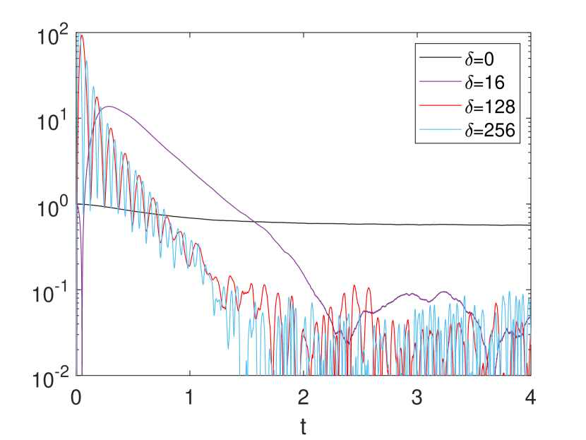
(a) Nonreversible Langevin dynamics (8).

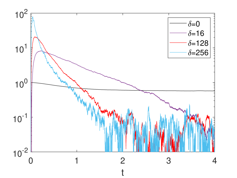
(b) Stratonovitch-perturbed Langevin dynamics (11).

Figure 1: Error evolution along time of the average over $M=10^{3}$ trajectories of the nonreversible and the Stratonovitch-perturbed Langevin dynamics for different sizes $\delta=0,16,128,256$ of the perturbation.

We consider the observable $\phi(x)=x_{1}^{2}+x_{2}^{2}$ and consider the estimator $\frac{1}{M}\sum_{i=1}^{M}\phi(X^{(i)}(t))\simeq{\mathbb{E}}(\phi(X(t))$. We take the initial condition $X_{0}=(0,0)$ and we plot for $M=10^{3}$ independent realisations $X^{(i)}(t),i=1,\ldots,M$ the error $|\frac{1}{M}\sum_{i=1}^{M}\phi(X^{(i)}(t))-\pi(\phi)|$ as a function of time $t\in[0,4]$. The solution is approximated using the simplest Euler-Maruyama method with very small stepsize $\Delta t=10^{-5}$ (considering the Itô formulation (18)). We observe that although the speed of the convergence ${\mathbb{E}}(\phi(X(t))\rightarrow\pi(\phi)$ as $t\rightarrow\infty$ is very slow for the standard overdamped Langevin dynamics (see the nearly horizontal black curve for $\delta=0$), both perturbations lead to an increase in the speed of the convergence to equilibrium (see the transient phase for small time $t$) while reducing the asymptotic variance (see the equilibrium phase for large time $t\geq 2$ where the oscillations are only due to Monte-Carlo errors), which corroborates Theorem 1.2 and Theorem 1.3. In addition, the Stratonovitch perturbation yields no oscillatory behavior in contrast to the nonreversible one (see Theorem 1.1). This feature renders the new sampling scheme more amenable to efficient numerical methods. This will be explored further in a future study.

References

- [1] C. Andrieu, N. de Freitas, A. Doucet, and M. I. Jordan. An introduction to MCMC for machine learning. Machine Learning, 50(1):5–43, Jan 2003.
- [2] A. B. Duncan, T. Lelièvre, and G. A. Pavliotis. Variance Reduction Using Nonreversible Langevin Samplers. J. Stat. Phys., 163(3):457–491, 2016.
- [3] A. B. Duncan, N. Nüsken, and G. A. Pavliotis. Using Perturbed Underdamped Langevin Dynamics to Efficiently Sample from Probability Distributions. J. Stat. Phys., 169(6):1098–1131, 2017.
- [4] A. B. Duncan, G. A. Pavliotis, and K. C. Zygalakis. Nonreversible Langevin samplers: Splitting schemes, analysis and implementation. ArXiv e-prints, 2017.
- [5] C.-R. Hwang, S.-Y. Hwang-Ma, and S.-J. Sheu. Accelerating Gaussian diffusions. Ann. Appl. Probab., 3(3):897–913, 1993.
- [6] C.-R. Hwang, S.-Y. Hwang-Ma, and S.-J. Sheu. Accelerating diffusions. Ann. Appl. Probab., 15(2):1433–1444, 2005.
- [7] T. Lelievre, F. Nier, and G. A. Pavliotis. Optimal non-reversible linear drift for the convergence to equilibrium of a diffusion. J. Stat. Phys., 152(2): 237–274 , 2013.
- [8] T. Lelièvre, M. Rousset, and G. Stoltz. Free energy computations. Imperial College Press, London, 2010. A mathematical perspective.
- [9] J. C. Mattingly, A. M. Stuart, and M. V. Tretyakov. Convergence of numerical time-averaging and stationary measures via Poisson equations. SIAM J. Numer. Anal., 48(2):552–577, 2010.
- [10] G. A. Pavliotis. Stochastic processes and applications, volume 60 of Texts in Applied Mathematics. Springer, New York, 2014. Diffusion processes, the Fokker-Planck and Langevin equations.
- [11] L. Rey-Bellet and K. Spiliopoulos. Irreversible langevin samplers and variance reduction: a large deviations approach. Nonlinearity, 28(7):2081, 2015.
- [12] L. Rey-Bellet and K. Spiliopoulos. Improving the convergence of reversible samplers. J. Stat. Phys., 164(3):472–494, 2016.
- [13] A. M. Stuart. Inverse problems: a Bayesian perspective. Acta Numer., 19:451–559, 2010.