A Privacy-preserving Disaggregation Algorithm
for Non-intrusive Management of Flexible Energy

Abstract

We consider a resource allocation problem involving a large number of agents with individual constraints subject to privacy, and a central operator whose objective is to optimizing a global, possibly non-convex, cost while satisfying the agents’ constraints. We focus on the practical case of the management of energy consumption flexibilities by the operator of a microgrid. This paper provides a privacy-preserving algorithm that does compute the optimal allocation of resources, avoiding each agent to reveal her private information (constraints and individual solution profile) neither to the central operator nor to a third party. Our method relies on an aggregation procedure: we maintain a global allocation of resources, and gradually disaggregate this allocation to enforce the satisfaction of private contraints, by a protocol involving the generation of polyhedral cuts and secure multiparty computations (SMC). To obtain these cuts, we use an alternate projections method à la Von Neumann, which is implemented locally by each agent, preserving her privacy needs. Our theoretical and numerical results show that the method scales well as the number of agents gets large, and thus can be used to solve the allocation problem in high dimension, while addressing privacy issues.

I INTRODUCTION

Motivation. Consider an operator of an electricity microgrid optimizing the joint production schedules of renewable and thermal power plants in order to satisfy, at each time period, the consumption constraints of its consumers. To optimize the costs and the renewables integration, this operator relies on demand response techniques, that is, taking advantage of the flexibilities of some of the consumers electric appliances—those which can be controlled without impacting the consumer’s confort, as electric vehicles or water heaters [1]. However, for privacy reasons, consumers are not willing to provide neither their consumption constraints nor their consumption profiles to a central operator or any third party, as this information could be used to induce private information such as their presence at home.

The global problem of the operator is to find an allocation of power (aggregate consumption) $\bm{p}=(p_{t})_{t}$ at each time period (resource) $t\in\mathcal{T}$, such that $\bm{p}\in\mathcal{P}$ (feasibility constraints of power allocation, induced by the power plants constraints). Besides, this aggregate allocation has to match an individual comsumption profile $\bm{x}_{n}=(x_{n,t})_{t\in\mathcal{T}}$ for each of the consumer (agent) $n\in\mathcal{N}$ considered. The problem can be written as follows:

$$\min_{\bm{x}\in\mathbb{R}^{N\times T},\ \bm{p}\in\mathcal{P}}f(\bm{p})$$ (1a)

$$\bm{x}_{n}\in\mathcal{X}_{n},\ \forall n\in\mathcal{N}$$ (1b)

$$\sum_{n\in\mathcal{N}}x_{n,t}=p_{t},\ \forall t\in\mathcal{T}\ ,$$ (1c)

The (aggregate) allocation $\bm{p}$ can be made public, that is, revealed to all agents. However, the individual constraint set $\mathcal{X}_{n}$ and individual profiles $\bm{x}_{n}$ constitute private information of agent $n$, and should not be reavealed to the operator or any third party.

The approach adopted in our paper is to deal with the problem (1) as two kinds of interdependent subproblems. The firsts are optimal resource allocation problems, or master problems, $\min_{\bm{p}\in\mathcal{P}^{(s)}}f(\bm{p})$ which consists in finding an aggregate allocation over $T$ resources ($\mathcal{P}^{(s)}\subset\mathcal{P}\subset\mathbb{R}^{T})$. The second kind is problems of finding the disaggregation of a given aggregate allocation $\bm{p}$, that is, to find an individual profile $\bm{x}_{n}$ for each agent (consumer) $n$ satisfying her individual constraint (1b), such that the aggregate of the profiles is the optimal allocation (1c) determined in a master problem.

Aside from the example above, ressource allocation problems (optimizing common resources shared by multiple agents) find many applications in energy [2, 1], logistics [3], distributed computing [4], health care [5] and telecommunications [6]. In these applications, several entities or agents (e.g. consumers, stores, tasks) share a common resource (energy, products, CPU time, broadband) which has a global cost for the system. For large systems composed of multiple agents, the dimension of the overall problem can be prohibitive and one can rely on decomposition and distributed approaches [7, 8, 9] to answer to this issue. Besides, agents’ individual constraints are often subject to privacy issues [10]. These considerations have paved the way to the development of privacy-preserving, or non-intrusive methods and algorithms, e.g. [11, 12].

In this work, we consider that each agent has a global demand constraint (e.g. energy demand or product quantity), which confers to the disaggregation problem the particular structure of a transportation polytope [13]: the sum over the agents is fixed by the aggregate solution $\bm{p}$, while the sum over the $T$ resources are fixed by the agent global demand constraint. Besides, individual constraints can also include minimal and maximal levels on each resource, as for instance electricity consumers require, through their appliances, a minimal and maximal power at each time period.

Main Results. The major contribution of the paper is to provide a non-intrusive and distributed algorithm (Algorithm 4) that computes an aggregated resource allocation $\bm{p}$, optimal solution of the—possibly nonconvex—optimization problem (1), along with feasible individual profiles $\bm{x}$ for agents, without revealing the individual constraints of each agent to a third party, either another agent or a central operator. The algorithm solves iteratively intances of master problem $\min_{\bm{p}\in\mathcal{P}^{(s)}}f(\bm{p})$ by constructing successive approximations $\mathcal{P}^{(s)}\subset\mathcal{P}$ of the aggregate feasible set of (1) for which a disaggregation exists, by adding a new constraint on $\bm{p}$ to $\mathcal{P}^{(s)}$, before solving the next master problem.

To identify whether or not disaggregation is feasible and to add a new constraint in the latter case, our algorithm relies on the alternating projections method (APM) [14, 15] for finding a point in the intersection of convex sets. Here, we consider the two following sets: on the one hand, the affine space defined by the aggregation to a given resource profile, and on the other hand, the set defined by all agents individual constraints (demands and bounds). As the latter is defined as a Cartesian product of each agent’s feasibility set, APM can operate in a distributed fashion. The sequence constructed by the APM converges to a single point if the intersection of the convex sets is nonempty, and it converges to a periodic orbit of length $2$ otherwise. Our key result is the following: if the APM converges to a periodic orbit, meaning that the disaggregation is not feasible, we construct from this orbit a polyhedral cut, i.e. a linear inequality satisfied by all feasible solutions $\bm{p}$ of the global problem (1), but violated from the current resource allocation (Thm. 4). Adding this cut to the master problem, we can recompute a new resource allocation and repeat this procedure until disaggregation is possible. Another major result stated in this paper is the explicit upper bound on the convergence speed of APM in our framework (Thm. 2), which is obtained by spectral graph theory methods, exploiting also geometric properties of transportation polytopes. This explicit speed shows a linear impact of the number of agents, which is a strong argument for the applicability of the method in large distributed systems.

Related Work. A standard approach to solve resource allocation problems in a distributed way is to use a Lagrangian (dual) decomposition technique [8, 16, 17]. Those techniques are generally used to decompose a large problems into several subproblems of small dimension. They may also be implemented in a way which preserve privacy (see Remark 2 in Sec. IV). However, Lagrangian decomposition methods are based on strong duality property, requiring global convexity hypothesis which are not satisfied in many practical problems (e.g. MILP, see Sec. V). On the contrary, our method can be used when the master allocation problem is not convex. In [2], the authors study a disaggregation problem similar to the one considered in this paper. Their results concern zonotopic sets, which is different from the structure we described in Sec. II. The APM has been the subject of several works in itself [15, 18, 19]. The authors of [20] provide general results on the convergence rate of APM for semi-algebraic sets. They show that the convergence is geometric for polyhedra. However, it is generally hard to compute explicitly the geometric convergence rate of APM, as this requires to bound the singular values of certain matrices arising from the polyhedral constraints. In [21], the authors provide an explicit convergence rate for APM on a class of polyhedra arising in submodular optimization. The sets they consider differ from the present transportation polytopes.

Structure. In Sec. II, we describe the master resource allocation problem and formulate the associated disaggregation problem. In Sec. III, we focus on the APM and state our main results. In Sec. IV, we apply these results to describe a non-intrusive version of APM (NI-APM) that is used to describe our non-intrusive algorithm for computing an optimal resource allocation. Finally, in Sec. V, we provide a concrete numerical example based on a MILP to model the management of a local electricity system (microgrid), and study numerically the influence of the number of agents on the time needed for convergence of our algorithm.

Notation. Vectors and matrices are denoted by bold fonts, $\bm{v}^{\top}$ denotes the transpose of $\bm{v}$, $\mathds{1}_{K}$ denotes the vector $(1\dots 1)^{\top}$ of size $K$, $\mathcal{U}([a,b])$ stands for the uniform distribution on $[a,b]$. We use $\left\|\bm{x}\right\|_{2}$ to denote the Frobenius norm $\left\|\bm{x}\right\|^{2}=\sum_{n,t}x_{n,t}^{2}$, and $P_{C}(.)$ to denote the Euclidean projection on a convex set $C$.

II Master problem and disaggregation structure

In this work, we suppose an operator wishes to determine an allocation of resources, represented by a $T$-dimensional vector $\bm{p}$, in order to minimize a global cost function $f$, for instance, an electricity power economic dispatch (or the allocation of different types of merchandise in warehouses in logistics applications) subject to a set of constraints described by a feasibility set $\mathcal{P}$. This problem can be nonconvex either because of nonconvex costs $f$ or because of a nonconvex feasible set $\mathcal{P}$ (see Sec. V). In the proposed method, the operator will consider master problems of the form:

$$\min_{\bm{p}\in\mathbb{R}^{T}}f(\bm{p})$$ (2a)

s.t. $$\bm{p}\in\mathcal{P}^{(s)}\ ,\vspace{-0.3cm}$$ (2b)

where the set $\mathcal{P}^{(s)}\subset\mathcal{P}$ is an aggregate approximation of disaggregation constraints. Indeed, the resource allocation $\bm{p}$ has to be shared between $N$ agents (e.g. consumers). Each agent has a global demand (total energy needed) $E_{n}$ and some lower and upper bounds on each of the resource $t\in\mathcal{T}$. The admissible set of profiles of agent $n$ is therefore:

$$\mathcal{X}_{n}\overset{\mathrm{def}}{=}\{\bm{x}_{n}\in\mathbb{R}^{T}|\ \bm{x}_{n}^{\top}\mathds{1}_{T}=E_{n}\text{ and }\forall t,\underline{x}_{n,t}\leq x_{n,t}\leq\overline{x}_{n,t}\}.$$ (3)

The disaggregation problem consists in finding individual profiles $\bm{x}=(x_{n,t})_{n,t}\in\mathbb{R}^{NT}$ of a given aggregated allocation $\bm{p}$ such that $\bm{x}_{n}$ is feasible for each agent $n$:

$$\textsc{Find }\bm{x}\in\mathcal{Y}_{\bm{p}}\cap\mathcal{X}$$ (4)

where $$\mathcal{Y}_{\bm{p}}\overset{\mathrm{def}}{=}\{\bm{y}\in\mathbb{R}^{NT}|\bm{y}^{\top}\mathds{1}_{N}=\bm{p}\}\text{ and }\mathcal{X}\overset{\mathrm{def}}{=}\prod_{n\in\mathcal{N}}\mathcal{X}_{n}\ .$$

Following (4), the disaggregated profile refers to $\bm{x}$, while the aggregated profile refers to the allocation $\bm{p}$.

Problem (4) may not always be feasible. Some necessary conditions for a disaggreagation to exist, obtained by summing the individual constraints on $\mathcal{N}$, are the following aggregated constraints:

$$\bm{p}^{\top}\mathds{1}_{T}=\bm{E}^{\top}\mathds{1}_{N}\text{ and }\ \bm{\underline{x}}^{\top}\mathds{1}_{N}\leq\bm{p}\leq\bm{\overline{x}}^{\top}\mathds{1}_{N}\ .$$ (5)

However, (inline,disable) are not sufficient conditions, as shown in Fig. 1 where the problem (4) is represented as a flow or circulation problem from source nodes $t\in\mathcal{T}$ to sink nodes $n\in\mathcal{N}$.

Indeed, with this circulation representation of the disaggregation problem (4), an immediate consequence of Hoffmann theorem [22, Thm. 3.18][23] is the following characterization of the disaggregation feasibility, which involves an exponential number of inequalities:

Theorem 1.

The disaggregation problem (4) is feasible (i.e. $\mathcal{X}\cap\mathcal{Y}_{\bm{p}}\neq\emptyset$) iff for any $\mathcal{T}_{\mathrm{in}}\subset\mathcal{T},\mathcal{N}_{\mathrm{in}}\subset\mathcal{N}$:

$$\sum_{t\notin\mathcal{T}_{\mathrm{in}}}p_{t}\leq\sum_{t\notin\mathcal{T}_{\mathrm{in}},n\in\mathcal{N}_{\mathrm{in}}}\overline{x}_{n,t}-\sum_{t\in\mathcal{T}_{\mathrm{in}},n\notin\mathcal{N}_{\mathrm{in}}}\underline{x}_{n,t}+\sum_{n\notin\mathcal{N}_{\mathrm{in}}}E_{n}.$$ (6)

The inequality (6) has a simple interpretation: the residual demand (the left hand side composed of demand and exports minus production) in $\mathcal{T}_{\mathrm{in}}\cup\mathcal{N}_{\mathrm{in}}$ cannot exceed the import capacity (right hand side of the inequality). One can see that, in the example of Fig. 1, inequality (6) does not hold when using the cut composed of the dashed nodes $p_{1}$ and $E_{1}$.

Figure 1: Example of disaggregation structure $(T=2,N=3)$, with $\bm{\underline{x}}=\bm{0}$ and $\bm{\overline{x}}:=\bm{1}$. Although the aggregate constraints (inline,disable) are satisfied, the disaggregation (4) of $\bm{p}$ is not feasible in this example (see Thm. 1).

There are two main reasons for which solving (1) is harder than solving (2) and (4) separately:

1. the dimension of (1) can be huge, as the number of agents $N$ can be really important, for instance in the example of individual consumers;

2. also, and this is the main motivation of this work, the information related to $(\bm{\overline{x}}_{n})_{n},(\bm{\underline{x}}_{n})_{n}$ and $(E_{n})_{n}$ might not be available to the centralized operator in charge of optimizing resources $\bm{p}$, as this information may be confidential and kept by each agent $n$, not willing to reveal it to any third party.

In the next sections, we provide a method that addresses those two issues, by considering subproblems (2) and (4) independently and iteratively, and exploiting the decomposable structure of problem (4).

III Alternate Projection Method (APM)

III-A Convergence of APM on Transportation Polytopes

In this section, we consider a fixed aggregated profile $\bm{p}$ and present the Von Neumann Alternate Projections Method (APM) [14] which solves the problem Eq. 4 of finding a point in the intersection $\mathcal{X}\cap\mathcal{Y}_{\bm{p}}$. In the remaining, we will often ommit $\bm{p}$ and just write $\mathcal{Y}$ to denote $\mathcal{Y}_{\bm{p}}$. The key idea of the method proposed in this paper is to use results of APM to generate a cut in the form of (6) and to add it as a new constraint in the master problem (2) to “improve” the aggregated profile $\bm{p}$ for the next iteration. As described in Algorithm 1, APM can be used to decompose (4) and only involves local operations.

1:Start with $\bm{y}^{(0)}$, $k=0$ , $\varepsilon_{\text{cvg}}$, a norm $\left\|.\right\|$ on $\mathbb{R}^{NT}$  

2:repeat

3:    $\bm{x}^{(k+1)}\leftarrow P_{\mathcal{X}}(\bm{y}^{(k)})$  

4:    $\bm{y}^{(k+1)}\leftarrow P_{\mathcal{Y}}(\bm{x}^{(k+1)})$  

5:    $k\leftarrow k+1$  

6:until $\left\|\bm{y}^{(k)}-\bm{y}^{(k-1)}\right\|<\varepsilon_{\text{cvg}}$

Algorithm 1 Alternate Projections Method (APM)

The convergence of Algorithm 1 is proved by Thm. 2:

Theorem 2 ([15]).

Let $\mathcal{X}$ and $\mathcal{Y}$ be two convex sets with $\mathcal{X}$ bounded, and let $(\bm{x}^{(k)})_{k}$ and $(\bm{y}^{(k)})_{k}$ be the two infinite sequences generated by Algorithm 1 with $\varepsilon_{\text{cvg}}=0$. Then there exists $\bm{x}^{\infty}\in\mathcal{X}$ and $\bm{y}^{\infty}\in\mathcal{Y}$ such that:

$$\bm{x}^{(k)}\underset{k\rightarrow\infty}{\longrightarrow}\bm{x}^{\infty}\ ,\quad\bm{y}^{(k)}\underset{k\rightarrow\infty}{\longrightarrow}\bm{y}^{\infty};$$ (7a)

$$\left\|\bm{x}^{\infty}-\bm{y}^{\infty}\right\|_{2}=\min_{{\bm{x}\in\mathcal{X},\bm{y}\in\mathcal{Y}}}\left\|\bm{x}-\bm{y}\right\|_{2}\ .$$ (7b)

In particular, if $\mathcal{X}\cap\mathcal{Y}\neq\emptyset$, then $(\bm{x}^{(k)})_{k}$ and $(\bm{y}^{(k)})_{k}$ converge to a same point $\bm{x}^{\infty}\in\mathcal{X}\cap\mathcal{Y}$.

If disaggregation is not feasible, Thm. 2 states that APM will “converge” to an orbit $(\bm{x}^{\infty},\bm{y}^{\infty})$ of period 2.

The convergence rate of APM has been the subject of several works [18, 20], and it strongly depends on the structure of the sets on which the projections are done: for instance, if the sets are polyhedral, [20, Prop. 4.2] shows that the convergence is geometric. However, there are very few cases in which an explicit upper bound on the convergence rate has been proved. In our case, we are able to obtain such a bound, as shown in the following theorem:

Theorem 3.

For the sets $\mathcal{X}$ and $\mathcal{Y}$ defined in (3-4), the two subsequences of alternate projections converge at a geometric rate to $\bm{x}^{\infty}\in\mathcal{X}$, $\bm{y}^{\infty}\in\mathcal{Y}$, with:

$$\|\bm{x}^{(k)}-\bm{x}^{\infty}\|_{2}\leq 2\|\bm{x}^{(0)}-\bm{x}^{\infty}\|_{2}\times\rho_{NT}^{k}$$

where $$\rho_{NT}\overset{\mathrm{def}}{=}1-\tfrac{1}{4}\left({N(T+1)^{2}(T-1)}\right)<1\ ,$$

Same inequalities hold for the convergence of $\bm{y}^{(k)}$ to $\bm{y}^{\infty}$.

Proof.

Appendix B provides a sketch of the proof.

Thm. 3 shows that the APM is efficient in our case of bounded transport polytopes. It shows that the number of iterations for a given accuracy grows linearly in the number of agents $N$.

As stated in (4), the set $\mathcal{X}$ is a Cartesian product $\prod_{n}\mathcal{X}_{n}$, so that the projection (13) can be computed by $N$ projections on $(\mathcal{X}_{n})_{n}$, which can be executed in parallel. Now, instead of solving the quadratic program by standard interior point methods and due to its particular structure, we can use the algorithm of Brucker [24], which has a complexity in $\mathcal{O}(T)$. On the other hand, $P_{\mathcal{Y}}(.)$ is a projection on an affine space, and the solution can be obtained explicitly as:

$$\forall n,t,\bm{y}_{n,t}=\bm{x}_{n,t}+\nu_{t}\text{ and }\bm{\nu}=\tfrac{1}{N}(\bm{p}-\bm{x}^{\top}\mathds{1}_{N})\ .$$ (8)

III-B Generation of a cut from APM iterates

Our key result is the following: in the case where APM converges to a periodic orbit $(\bm{x}^{\infty},\bm{y}^{\infty})$ with $\bm{x}^{\infty}\neq\bm{y}^{\infty}$ (see Thm. 2), we obtain from $(\bm{x}^{\infty},\bm{y}^{\infty})$ an inequality (6) that is violated by $\bm{p}$:

Theorem 4.

For the sets $\mathcal{X}$ and $\mathcal{Y}$ defined in (3-4) and if $\mathcal{X}\cap\mathcal{Y}=\emptyset$ , the following sets given by the limit orbit $(\bm{x}^{\infty},\bm{y}^{\infty})$ defined in Thm. 2:

$$\mathcal{T}_{0}\overset{\mathrm{def}}{=}\{t|p_{t}>\textstyle\sum_{n\in\mathcal{N}}x^{\infty}_{n,t}\}$$ (9a)

$$\mathcal{N}_{0}\overset{\mathrm{def}}{=}\{n\ |E_{n}-\textstyle\sum_{t\notin\mathcal{T}_{0}}\underline{x}_{n,t}-\sum_{t\in\mathcal{T}_{0}}\overline{x}_{n,t}<0\}\$$ (9b)

define a Hoffman cut of form (6) violated by $\bm{p}$, that is:

$$\sum_{n\in\mathcal{N}_{0}}E_{n}-\sum_{t\in\mathcal{T}_{0}}p_{t}+\sum_{t\in\mathcal{T}_{0},n\notin\mathcal{N}_{0}}\overline{x}_{n,t}-\sum_{t\notin\mathcal{T}_{0},n\in\mathcal{N}_{0}}\underline{x}_{n,t}<0\ .$$ (10)

This cut can be reformulated in terms of $\mathds{1}_{N}^{\top}\bm{x}^{\infty}$ as:

$$\mathrm{A}_{\mathcal{T}_{0}}<\sum_{t\in\mathcal{T}_{0}}p_{t}\text{\ with }\mathrm{A}_{\mathcal{T}_{0}}\overset{\mathrm{def}}{=}\sum_{t\in\mathcal{T}_{0}}\sum_{n\in\mathcal{N}}x^{\infty}_{n,t}.$$ (11)

Proof.

Appendix A gives the sketch of the proof of Thm. 4. The complete proofs will be given elsewhere.

One can see that, intuitively, $\mathcal{N}_{0}$ is the subset associated to $\mathcal{T}_{0}$ that minimizes the right hand side of (6). Note that Thm. 4 gives an alternative constructive proof of Hoffman circulation’s theorem (Thm. 1) in the case of a bipartite graph of the form of Fig. 1. Moreover, in the case where the disaggregation problem (4) is not feasible, the negation of equation (11) provides a new valid constraint as a condition for the existence of a disaggreagated profile of $\bm{p}$. This constraint can be used in the master problem (2) to update the vector of resources $\bm{p}$ for the next iteration. This constraint only involves the aggregate information $\mathds{1}_{N}^{\top}\bm{x}^{\infty}$ on the users profile. To make the process fully non-intrusive, we explain in Sec. IV-A how the operator can compute this constraint without making the agents reveal their profiles $(\bm{x}^{\infty}_{n})_{n\in\mathcal{N}}$.

IV Non-intrusive Projections and Computation of Disaggregated Optimal Resources

IV-A Non-Intrusive Alternate Projections Method (NI-APM)

Because of the particular structure of the problem, the projections in APM can be computed separately by the operator and the agents. The projection $P_{\mathcal{Y}}$ is made by the operator, which only requires to know $\bm{p}$ and the aggregate profile $\bm{x}^{\top}\mathds{1}_{N}$ according to from (8). The projection $P_{\mathcal{X}}$ on $\mathcal{X}=\prod_{n}\mathcal{X}_{n}$ is executed in parallel by each agent: $n$ computes $P_{\mathcal{X}_{n}}$ which only needs her private information $E_{n}$ and $\bm{\overline{x}}_{n},\bm{\underline{x}}_{n}$. However, in the way APM is described in Algorithm 1, the operator and the agents still need to exchange the iterates $\bm{x}^{(k)},\bm{y}^{(k)}$ at each step. To avoid the transmission of agents’ profiles to the operator, we use a secure multiparty computation (SMC) technique (see [25]) which enables the operator to obtain the aggregate profile $\SS^{(k)}:=\mathds{1}_{N}^{\top}\bm{x}^{(k)}$ in a non-intrusive manner, as described in Algorithm 2.

The main idea of SMC is that, instead of sending her profile $\bm{x}_{n}$, agent $n$ splits $x_{n,t}$ for each $t$ into $N$ random parts $(s_{n,t,m})_{m}$, according to an uniform distribution and summing to $\bm{x}_{n,t}$ (Lines 3-4). Thus, each part $s_{n,t,m}$ taken individually does not reveal any information on $\bm{x}_{n}$ nor on $\mathcal{X}_{n}$, and can be sent to agent $m$. Once all exchanges of parts are completed (Line 5), and $n$ has herself received the parts from other agents, agent $n$ computes a new aggregate quantity $\bm{\sigma}_{n}$ (Line 8), which does not contain either any information about any of the agents, and sends it to the operator (Line 9). The operator can finally compute the quantity $\SS=\bm{x}^{\top}\mathds{1}_{N}=\bm{\sigma}^{\top}\mathds{1}_{N}$.

1:Each agent has a profile $(\bm{x}_{n})_{n\in\mathcal{N}}$ 

2:for each agent $n\in\mathcal{N}$ do

3:    Draw $\forall t,(s_{n,t,m})_{m=1}^{N-1}\in\mathcal{U}([0,A]^{N-1})$  

4:    and set $\forall t,s_{n,t,N}\overset{\mathrm{def}}{=}{x}_{n,t}-\sum_{m=1}^{N-1}s_{n,t,m}$ 

5:    Send $(s_{n,t,m})_{t\in\mathcal{T}}$ to agent $m\in\mathcal{N}$  

6:done

7:for each agent $n\in\mathcal{N}$ do

8:    Compute $\forall t,\sigma_{n,t}=\sum_{m\in\mathcal{N}}s_{m,t,n}$  

9:    Send $(\sigma_{n,t})_{t\in\mathcal{T}}$ to operator  

10:done

11:Operator computes $\SS=\sum_{n\in\mathcal{N}}\bm{\sigma}_{n}$  

Algorithm 2 SMC of Aggregate (SMCA) $\sum_{n\in\mathcal{N}}\bm{x}_{n}$

Remark 1.

As $\bm{\sigma}_{n},$ and $\bm{s}_{n}$ are random by construction, an eavesdropper aiming to learn the profile $\bm{x}_{n}$ of $n$ has no choice but to intercept all the communications of $n$ to all other agents (to learn $(s_{n,t,m})_{m\neq n}$ and $(s_{m,t,n})_{m\neq n}$) and to the operator (to learn $\sigma_{n}$). To increase the confidentiality of the procedure, one could use any encryption scheme (such as RSA [26]) for all communications involved in Algorithm 2.

We can use this non-intrusive computation of aggregate $\SS$ in APM to obtain a non-intrusive algorithm NI-APM (Algorithm 3) in which agents do not reveal neither their profiles nor their constraints to the operator.

1:Start with $\bm{y}^{(0)}$, $k=0$, $\varepsilon_{\text{cvg}},\varepsilon_{\text{dis}}$, norm $\left\|.\right\|$ on $\mathbb{R}^{NT}$  

2:repeat

3:    for each agent $n\in\mathcal{N}$ do

4:        ${\bm{x}}_{n}^{(k)}\leftarrow P_{\mathcal{X}_{n}}({\bm{y}}_{n}^{(k-1)})$  

5:    done

6:    Operator obtains $\SS^{(k)}\leftarrow$SMCA($\bm{x}^{(k)}$) (cf Algo.2)  

7:    and sends $\bm{\nu}^{(k)}:=\frac{1}{N}(\bm{p}-\SS^{(k)})\in\mathbb{R}^{T}$ to agents $\mathcal{N}$  

8:    for each agent $n\in\mathcal{N}$ do

9:        Compute $\bm{y}_{n}^{(k)}\leftarrow\bm{x}_{n}^{(k)}+\bm{\nu}^{(k)}$  

10:    done

11:    $k\leftarrow k+1$  

12:until  $\left\|\bm{x}^{(k)}-\bm{x}^{(k-1)}\right\|<\varepsilon_{\text{cvg}}$

13:if  $\left\|\bm{x}^{(k)}-\bm{y}^{(k)}\right\|\leq\varepsilon_{\text{dis}}$ then $\quad\triangleright$ found a $\varepsilon_{\text{dis}}$-solution of the disaggregation problem

14:    Each agent adopts profile $\bm{x}_{n}^{(k)}$  

15:    return Disag $\leftarrow$ True  

16:else$\quad\triangleright$ have to find a valid constraint violated by $\bm{p}$

17:    Operator computes $\mathcal{T}_{0}\leftarrow\{t\in\mathcal{T}\ |\ \tfrac{3}{2}B\varepsilon_{\text{cvg}}<\nu_{t}^{(k)}\}$  

18:    Operator computes $\mathrm{A}_{\mathcal{T}_{0}}\overset{\mathrm{def}}{=}\sum_{t\in\mathcal{T}_{0}}\mathds{1}_{N}^{\top}\bm{\sigma}_{t}^{(k)}$  

19:    if $\mathrm{A}_{\mathcal{T}_{0}}-\sum_{t\in\mathcal{T}_{0}}\bm{p}_{t}<0$ then

20:        return Disag $\leftarrow$ False, $\mathrm{A}_{\mathcal{T}_{0}}$ 

21:    else$\quad\triangleright$ need to run APM with higher precision

22:        Return to Line 2 with $\varepsilon_{\text{cvg}}\leftarrow\varepsilon_{\text{cvg}}/2$  

23:    end 

24:end 

Algorithm 3 Non-intrusive APM (NI-APM)

One can see that $\bm{x}$ and $\bm{y}$ computed in Lines 4 and 9 in Algorithm 3 correspond to the projections computed in the original APM Algorithm 1. In Algorithm 3, the operator obtains the aggregate profile $\SS^{(k)}$ (Line 6), computes and sends the corrections $\bm{\nu}^{(k)}$ to all agents (Line 7). Then, each agent can compute locally the projection $\bm{y}_{n}^{(k)}=P_{\mathcal{Y}}(\bm{x}_{n}^{(k)})$ by applying the correction $\bm{\nu}^{(k)}$ (Line 9).

Using (8), we get $\bm{\nu}^{(k)}\rightarrow\bm{\nu}^{\infty}\overset{\mathrm{def}}{=}\tfrac{1}{N}(\bm{p}-\mathds{1}_{N}^{\top}\bm{x}^{\infty})$. Thm. 4 uses this limit value through ${\mathcal{T}_{0}}^{\infty}\overset{\mathrm{def}}{=}\{t\in\mathcal{T}|0<\nu_{t}^{\infty}\}$. Yet, from APM, one can only access to $\bm{\nu}^{(k)}$ and thus to the approximation $\mathcal{T}_{0}$, computed on Line 17), where $B$ is a pre-defined constant. However, we show that for $\varepsilon_{\text{cvg}}$ small enough and a well-chosen value of $B$, we obtain $\mathcal{T}_{0}=\mathcal{T}_{0}^{\infty}$, so that we get the termination result:

Proposition 1.

For $B>(1-\rho_{NT})^{-1}$, Algorithm 3 terminates in finite time.

The termination of the loop Lines 2-12 is ensured by Thm. 3. In the case where $\left\|\bm{x}^{(k)}-\bm{y}^{(k)}\right\|\leq\varepsilon_{\text{dis}}$, Algorithm 3 terminates. Otherwise, if $\left\|\bm{x}^{\infty}-\bm{y}^{\infty}\right\|>\varepsilon_{\text{dis}}$, then Algorithm 3 terminates (i.e. Line 19 is True and a new cut is found) as soon as $B\varepsilon_{\text{cvg}}<\min\left\{\frac{\left\|\bm{x}^{\infty}-\bm{y}^{\infty}\right\|_{1}}{2\sqrt{N}},\ \frac{2}{5}\underline{\nu}\right\}$, where $\underline{\nu}\overset{\mathrm{def}}{=}\min\{|\nu_{t}^{\infty}|>0\}$ and with $\left\|.\right\|=\left\|.\right\|_{2}$. The complete proof is ommited here.

In practice, we can start with a large $\varepsilon_{\text{cvg}}$ to obtain the first constraints while avoiding useless computation, and then half $\varepsilon_{\text{cvg}}$ if needed (Line 22) until the termination condition holds.

Remark 2.

SMC techniques could also be used to implement non-intrusive Lagrangian decomposition methods. However, these methods rely on a convexity hypothesis that we do not need in the proposed method.

IV-B Non-intrusive Disaggregation of Optimal Allocation

In this section, we describe a method to compute a solution of the global problem (1), that is, an optimal resource allocation $\bm{p}$ for which a disaggregation exists, along with an associated disaggregated profile $\bm{x}_{n}$ for each agent $n$. This computation is done in a non-intrusive manner: the operator in charge of $\bm{p}$ does not have access neither to the bounding constraints $\bm{\overline{x}}$ and $\bm{\underline{x}}$ of the agents nor to the agents disaggregated profile $\bm{x}$, as detailed in Algorithm 4 below.

1:$s=0$ , $\mathcal{P}^{(0)}=\mathcal{P}$ ; Disag = False  

2:while Not Disag  do

3:    Compute $\bm{p}^{(s)}=\arg\min_{\bm{p}\in\mathcal{P}_{\text{cs}}^{(s)}}\bm{p}$  

4:     Disag $\leftarrow$ NI-APM($\bm{p}^{(s)}$)  

5:    if  Disag  then

6:        Operator adopts $\bm{p}^{(s)}$  

7:    else

8:        Obtain $\mathcal{T}_{0}^{(s)},\mathrm{A}_{\mathcal{T}_{0}}^{(s)}$ from NI-APM($\bm{p}^{(s)}$)  

9:        $\mathcal{P}^{(s+1)}\leftarrow\mathcal{P}^{(s)}\cap\{\bm{p}|\sum_{t\in\mathcal{T}_{0}^{(s)}}p_{t}\leq\mathrm{A}_{\mathcal{T}_{0}}^{(s)}\}$  

10:    end 

11:    $s\leftarrow s+1$ 

12:done 

Algorithm 4 Non-intrusive Optimal Disaggregation

Algorithm 4 iteratively calls NI-APM (Algorithm 3) and in case disaggregation is not possible (Line 7), a new constraint is added (Line 9), obtained from the quantity $\mathrm{A}_{\mathcal{T}_{0}}$ defined in (11), to the resource problem (2). This constraint is an inequality on $\bm{p}$ and thus does not reveal significant individual information to the operator. The algorithm stops when disaggregation is possible (Line 5). The termination of Algorithm 4 is ensured by the following property and the form of the constraints added (10):

Proposition 2.

Algorithm 4 stops after a finite number of iterations, as at most $2^{T}$ constraints (Line 9) can be added to the master problem (Line 3).

Although there exist some instances with an exponential number of independent constraints, this does not jeopardize the proposed method: in practice, the algorithm stops after a very small number of constraints added (see the example of Sec. V). Intuitively, we will only add constraints “supporting” the optimal allocation $\bm{p}$.

Thus, Algorithm 4 is a method which enables the operator to compute a resource allocation $\bm{p}$ and the $N$ agents to adopt profiles $(\bm{x}_{n})_{n}$, such that $(\bm{x},\bm{p})$ solves the global problem (1), and the method ensures that both:

1. the information relative to each agent constraints (upper bounds $\bm{\overline{x}}_{n}$, lower bounds $\bm{\underline{x}}_{n}$, demand $E_{n}$);

2. the final disaggregated profile $\bm{x}_{n}$ (as well as the iterates $(\bm{x}^{(k)})_{k}$ and $(\bm{y}^{(k)})_{k}$ in NI-APM)

are kept confidential by agent $n$ and can not be induced by a third party (either the operator or any other agent $m\neq n$).

V Application to Management of a Microgrid

We apply the proposed method to solve a nonconvex distributed problem in the energy field. We consider a microgrid [27] composed of N electricity consumers with flexible appliances (such as electric vehicles or water heaters), a photovoltaic (PV) power plant and a conventional generator.

V-A Mixed Integer Problem Formulation

The operator responsible of the microgrid aims at satisfying the demand constraints of consumers over a set of time periods $\mathcal{T}=\{1,\dots,T\}$, while minimizing the energy cost for the community. We have the following characteristics:

• the PV plant generates a nondispatchable power profile $(p^{\textsc{pv}}_{t})_{t\in\mathcal{T}}$ at marginal cost zero;

• the conventional generator has a starting cost $C^{\textsc{st}}$, minimal and maximal power production $\underline{p}^{g},\overline{p}^{g}$, and piecewise-linear and continuous generation cost function $p^{g}\mapsto f(p^{g})$:

  $$f(p^{g})=\alpha_{k}+c_{k}p^{g},\text{ if }p^{g}\in\mathcal{I}_{k}\overset{\mathrm{def}}{=}[\theta_{k-1},\ \theta_{k}[,\ k=1\dots K,$$

  where $\theta_{0}\overset{\mathrm{def}}{=}0$ and $\theta_{K}\overset{\mathrm{def}}{=}\overline{p}^{g}$;

• each agent $n\in\mathcal{N}$ has some flexible appliances which require a global energy demand $E_{n}$ on $\mathcal{T}$, and has consumption constraints on the total household consumption, on each time period $t\in\mathcal{T}$, that are formulated with $\bm{\underline{x}}_{n},\bm{\overline{x}}_{n}$. These parameters are confidential because they could for instance contain some information on agent $n$ habits.

The master problem (2) can be written as a MILP (12):

$$\min_{\bm{p},\bm{p}^{g},(\bm{p}^{g}_{k}),(\bm{b}_{k}),\bm{b^{\textsc{on}}},\bm{b^{\textsc{st}}}}\sum_{t\in\mathcal{T}}\Big{(}\alpha_{1}b^{\textsc{on}}_{t}+\sum_{k}c_{k}{p^{g}_{k}}_{t}+C^{\textsc{st}}b^{\textsc{st}}_{t}\Big{)}$$ (12a)

$$p^{g}_{t}=\textstyle\sum_{k=1}^{K}p^{g}_{k,t},\ \forall t\in\mathcal{T}$$ (12b)

$$b_{1,t}\theta_{1}\leq p^{g}_{1,t}\leq\theta_{1},\ \forall t\in\mathcal{T}$$ (12c)

$$b_{2,t}(\theta_{2}-\theta_{1})\leq p^{g}_{2,t}\leq b_{1,t}(\theta_{2}-\theta_{1}),\ \forall t\in\mathcal{T}$$ (12d)

$$\vdots\hskip 85.35826pt\vdots$$ (12e)

$$0\leq p^{g}_{K,t}\leq b_{K-1,t}(\theta_{K}-\theta_{K-1}),\ \forall t\in\mathcal{T}$$ (12f)

$$b^{\textsc{st}}_{t}\geq b^{\textsc{on}}_{t}-b^{\textsc{on}}_{t-1},\ \forall t\in\{2,\dots,T\}$$ (12g)

$$\underline{p}^{g}b^{\textsc{on}}_{t}\leq p^{g}_{t}\leq\overline{p}^{g}b^{\textsc{on}}_{t},\ \forall t\in\mathcal{T}$$ (12h)

$$b^{\textsc{on}}_{t},b^{\textsc{st}}_{t},b_{1,t},\dots,b_{K-1,t}\in\{0,1\},\ \forall t\in\mathcal{T}$$ (12i)

$$\bm{p}\leq\bm{p}^{\textsc{pv}}+\bm{p}^{g}$$ (12j)

$$\bm{p}^{\top}\mathds{1}_{T}=\bm{E}^{\top}\mathds{1}_{N}$$ (12k)

$$\bm{\underline{x}}^{\top}\mathds{1}_{N}\leq\bm{p}\leq\bm{\overline{x}}^{\top}\mathds{1}_{N}\ .$$ (12l)

In this formulation (12b-12f) are a mixed integer formulation of the generation cost function $f$: one can show that the boolean variable $b_{k,t}$ is equal to one iff $p^{g}_{k,t}\geq\theta_{k}$ for each $k\in\{1,\dots,K-1\}$. Note that only $\alpha_{1}$ appears in (12a) because of the continuity assumption on $f$.

Constraints (12g-12h) ensure the on/off and starting constraints of the power plant, (12j) ensures that the power allocated to consumption is not above the total production, and (12k-12l) are the aggregated feasibility conditions already referred to in (inline,disable). Note that more complex and realistic MILP models exist for power plants (e.g. [28]), but with the same structure than (12). The nonconvexity of (12) comes from the existence of starting costs and on minimal the power constraint, which makes necessary to use boolean state variables $b^{\textsc{st}},b^{\textsc{on}}$.

V-B Parameters

We simulate the problem described above for different values of $N\in\{2^{4}$,$2^{5}$, $2^{6}$,$2^{7}$,$2^{8}\}$ and one hundred instances with random parameters for each value of $N$. A scaling factor $\kappa_{N}\overset{\mathrm{def}}{=}N/20$ is applied on parameters to ensure that production capacity is large enough to meet consumers demand. The parameters are chosen as follows:

• $T=24$ (hours of a day);

• production costs: $K=3$ , $\theta=[0,70,100,300]\kappa_{N},\bm{c}=[0.2,0.4,0.5]$, $\underline{p}^{g}=50\kappa_{N},\overline{p}^{g}=300\kappa_{N}$, $\alpha_{1}=4$ and $C^{\textsc{st}}=15$;

• photovoltaic: $p^{\textsc{pv}}_{t}=\left[50(1-\mathrm{cos}(\frac{(t-6)2\pi}{16})+\mathcal{U}([0,10])\right]\kappa_{N}$ for $t\in\{6,\dots,20\}$, $p^{\textsc{pv}}_{t}=0$ otherwise (see Fig. 3);

• for consumption parameters, we used $\underline{x}_{n,t}\sim\mathcal{U}([0,10])$, $\overline{x}_{n,t}\sim\mathcal{U}([0,5])+\underline{x}_{n,t}$ and $E_{n}\sim\mathcal{U}([\mathds{1}_{T}^{\top}\bm{\underline{x}}_{n},\mathds{1}_{T}^{\top}\bm{\overline{x}}_{n}])$, so that individual feasibility ($\mathcal{X}_{n}\neq\emptyset$) is ensured.

$N=$	$2^{4}$	$2^{5}$	$2^{6}$	$2^{7}$	$2^{8}$
# master pb.	193.6	194.1	225.5	210.9	194.0
# projs.	9506.9	15366.7	24319.3	26537.5	26646.4

Table I: number of subproblems solved (average on 100 instances)

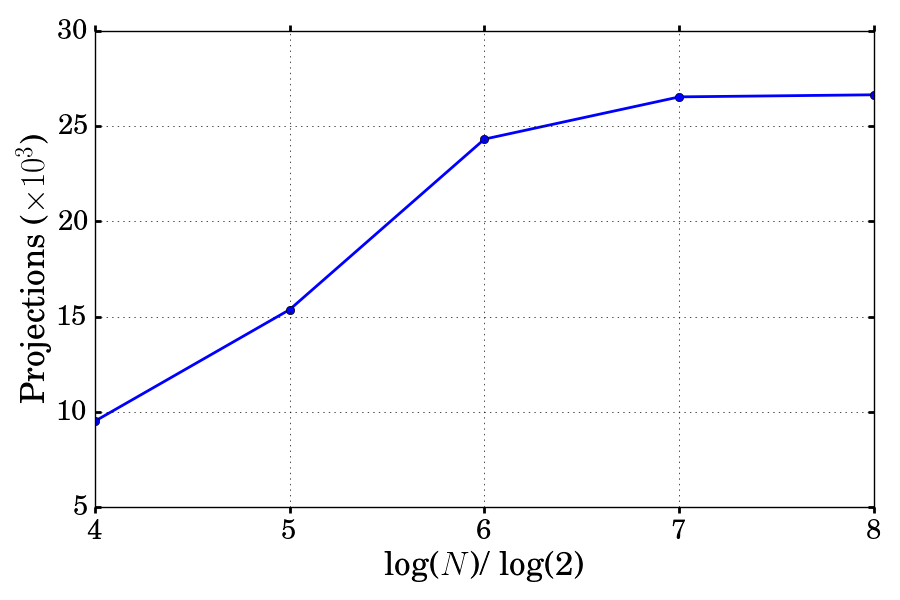
Figure 2: Total number of computed projections for different values of $N$. We observe that the number of agents $N$ has a sublinear impact on the total number of projections needed.

V-C A limited impact of the number $N$ of agents

We implement Algorithm 4 using Python 3.5. The MILP (12) is solved using Cplex Studio 12.6 and Pyomo interface. Simulations are run on a single core of a cluster at 3GHz. For the convergence criteria (see Lines 12 and 13 of Algorithm 3), we use $\varepsilon_{\text{dis}}=0.01$ with the operator norm defined by $\left\||\bm{x}|\right\|=\max_{n\in\mathcal{N}}\sum_{t}|x_{n,t}|$ (to avoid the $\sqrt{N}$ factor in the convergence criteria appearing with $\left\|.\right\|_{2}$), and starts with $\varepsilon_{\text{cvg}}=0.1$. The largest instances took around 10 minutes to be solved in this configuration and without parallel implementation. As the CPU time needed depend on the cluster load, it is not a reliable indicator of the influence on $N$ on the complexity of the problems. Moreover, one advantage of the proposed method is that the projections in APM can be computed locally by each agent in parallel, which could not be implemented here for practical reasons.

Tab. I gives two robust indicators of the influence of $N$ on the problem complexity: the number of master problems solved and the total number of projections computed, on average over the hundred instance for each value of $N$:

• one observes that the number of master problems solved (MILP (12) ), which corresponds to the number of constraints or “cuts” added to the master problem, remains almost constant when $N$ increases;

• in all instances, this number is way below the upper bound of $2^{24}>1,6\times 10^{7}$ possible constraints (see proof of Prop. 2), which suggests that only a polynomial number of constraints are added in practice;

• the average total number of projections computed for each instance (total number of iterations of the while loop of Algorithm 3, Line 2 over all calls of APM in the instance) increases in a sublinear way, as illustrated in Fig. 2, which is even better that one could expect from the upper bound given in Thm. 3.

Figure 3: Example of optimal resource allocation (power production $\bm{p}=\bm{p}^{\textsc{pv}}+\bm{p}^{g}$) in the example of Sec. IV, with $N=20$ agents. Exploiting consumption flexibilities, the consumption is higher during the PV production periods.

VI Conclusion

We provided a non-intrusive algorithm that enables to compute an optimal resource allocation, solution of a–possibly nonconvex–optimization problem, and affect to each agent an individual profile satisfying a global demand and lower and upper bounds constraints. Our method uses local projections and works in a distributed fashion. Hence, it ensures that the problem is not affected by the high dimension relative to the large number of agents, and that it is privacy-preserving, as agents do not need to reveal any information on their constraints or their individual profile to a third party. Several extensions and generalizations can be considered. First, we could generalize the abstract circulation problem on the bipartite graph depicted in Fig. 1 to an arbitrary network, where the set of nodes is partitioned in $K$ parts defining $K$ sets on which we could make alternating projections. Second, our method relies on the particular structure obtained from the form of constraints. Although these kind of constraints are widely used to model many practical situations, it would also be useful to obtain similar results for arbitrary (or polyhedral) agents constraints. Last, a deeper complexity analysis, with a thinner upper bound on the maximal number of constraints (cuts) added in the algorithm (see Prop. 2 and Tab. I) would constitute interesting results.

Appendix A Proof of Prop. 3

To show Thm. 4, we formulate the projections $P_{\mathcal{X}}$ and $P_{\mathcal{Y}}$ as the solutions of the constrained quadratic programs:

$$\min_{\bm{x}\in\mathbb{R}^{NT}}\frac{1}{2}\left\|\bm{x}-\bm{y}\right\|_{2}^{2}$$ (13a)

$$\ {\bm{x}}\mathds{1}_{T}=\bm{E} (\bm{\lambda})$$ (13b)

$$\ \bm{\underline{x}}\leq{\bm{x}}\leq\bm{\overline{x}} (\bm{\underline{\mu}},\bm{\overline{\mu}})$$ (13c)

and:

$$\min_{\bm{y}\in\mathbb{R}^{NT}}\frac{1}{2}\left\|\bm{x}-\bm{y}\right\|_{2}^{2}$$ (14a)

$${\bm{y}}^{\top}\mathds{1}_{N}=\bm{p} (\bm{\nu})\ ,$$ (14b)

where $\bm{\lambda},\bm{\underline{\mu}},\bm{\overline{\mu}},\bm{\nu}$ are the Lagrangian multipliers associated to the constraints. Although there is no such explicit characterization of the solution of (13) as the one (8) given for (14), we can obtain the following properties:

Proposition 3.

Suppose that $\mathcal{X}\cap\mathcal{Y}=\emptyset$ and consider the sets $\mathcal{T}_{0}$ and $\mathcal{N}_{0}$ given by (9). Then we have the following:

1. $\forall t\in\mathcal{T}_{0},\forall n\notin\mathcal{N}_{0},\ y^{\infty}_{n,t}\geq\overline{x}_{n,t}$ and $x^{\infty}_{n,t}=\overline{x}_{n,t}$ ;

2. $\forall n\in\mathcal{N}_{0},\lambda_{n}<0$ ;

3. $\forall t\notin\mathcal{T}_{0},\forall n\in\mathcal{N}_{0},\ x^{\infty}_{n,t}=\underline{x}_{n,t}$  ;

4. the sets $\mathcal{T}_{0},\mathcal{T}_{0}^{c}$, $\mathcal{N}_{0}$ and $\mathcal{N}_{0}^{c}$ are nonempty.

The proof of Prop. 3 relies on the KKT optimality conditions associated to (13) and (14). Then we use Prop. 3 and the convergence condition to prove Thm. 4:

$$\sum_{n\in\mathcal{N}_{0}}E_{n}+\sum_{t\in\mathcal{T}_{0},n\notin\mathcal{N}_{0}}\overline{x}_{n,t}-\sum_{t\notin\mathcal{T}_{0},n\in\mathcal{N}_{0}}\underline{x}_{n,t}-\sum_{t\in\mathcal{T}_{0}}p_{t}$$

$$=\sum_{t\in\mathcal{T}_{0}}\left(\sum_{n\in\mathcal{N}}x^{\infty}_{n,t}-\sum_{n\in\mathcal{N}}y^{\infty}_{n,t}\right)=\sum_{t\in\mathcal{T}_{0}}\left(\sum_{n\in\mathcal{N}}-\nu^{\infty}_{t}\right)$$

$$=\sum_{t\in\mathcal{T}_{0}}\left(-\sum_{n\in\mathcal{N}}\left|x^{\infty}_{n,t}-y^{\infty}_{n,t}\right|\right)=-\frac{\left\|\bm{x}^{\infty}-\bm{y}^{\infty}\right\|_{1}}{2}<0\ ,$$

where the last equality comes from $\sum_{t\in\mathcal{T}_{0}}\sum_{n\in\mathcal{N}}({x_{E}}_{n,t}-{x_{P}}_{n,t})=0$. The compact form (11) also follow from Prop. 3:

$$A_{\mathcal{T}_{0}}(\bm{x}) =\sum_{n\in\mathcal{N}_{0}}E_{n}+\sum_{t\in\mathcal{T}_{0},n\notin\mathcal{N}_{0}}\overline{x}_{n,t}-\sum_{t\notin\mathcal{T}_{0},n\in\mathcal{N}_{0}}\underline{x}_{n,t}$$

$$=\sum_{n\in\mathcal{N}_{0},t\in\mathcal{T}_{0}}x^{\infty}_{n,t}+\sum_{t\in\mathcal{T}_{0},n\notin\mathcal{N}_{0}}x^{\infty}_{n,t}=\sum_{t\in\mathcal{T}_{0}}\sum_{n\in\mathcal{N}}x^{\infty}_{n,t}\ .$$

Appendix B Proof of Thm. 2

For this analysis, we use the space $\mathbb{R}^{NT}=\mathbb{R}^{T}\times\dots\times\mathbb{R}^{T}$, where the $(n-1)T+1$ to $nT$ coordinates correspond to agent $n$, for $1\leq n\leq N$. We make use of the following results:

Lemma 1 ([21]).

For APM on polyhedra $\mathcal{X}$ and $\mathcal{Y}$, the sequences $(\bm{x}^{(k})_{k}$ and $(\bm{y}^{(k})_{k}$ converge at a geometric rate, where the rate is bounded by the maximal value of the square of the cosine of the Friedrichs angle $c_{F}(U,V)$ between a face $U$ of $\mathcal{X}$ and a face $V$ of $\mathcal{Y}$, where $c_{F}(U,V)$ is given by:

$$\begin{split}c_{F}(U,V)=\sup\{&u^{T}v\ |\left\|u\right\|\leq 1,\left\|v\right\|\leq 1\\ &u\in U\cap(U\cap V)^{\perp},v\in V\cap(U\cap V)^{\perp}\}.\end{split}$$

Lemma 2 ([21]).

Let $A$ and $B$ be matrices with orthonormal rows and with equal numbers of columns and $\Lambda_{\rm{sv}}(AB^{\top})$ the set of singular values of $AB^{\top}$. Then if $\Lambda_{\rm{sv}}(AB^{\top})=\{1\}$, then $c_{F}(\rm{Ker}(A),\rm{Ker}(B))=0$. Otherwise, $c_{F}(\rm{Ker}(A),\rm{Ker}(B))=\max_{\lambda<1}\{\lambda\in\Lambda_{\rm{sv}}(AB^{\top})\}$.

In our case, the polyhedra $\mathcal{Y}$ is an affine subspace $\mathcal{Y}=\{\bm{x}\in\mathbb{R}^{NT}\ |A\bm{x}=\sqrt{N}^{-1}\bm{1}_{T}\}$ with $A\overset{\mathrm{def}}{=}\sqrt{N}^{-1}J_{1,N}\otimes I_{T}$, where $\otimes$ denotes the Kronecker product. The matrix $A$ has orthonormal rows and the direction of $\mathcal{Y}$ is $\text{Ker}(A)$.

Describing the faces $\mathcal{X}$ is more complex. We have a polyhedral description of $\mathcal{X}$, and the faces of $\mathcal{X}$ are subsets of the collection of affine subspaces indexed by $\ (\overline{\mathcal{T}}_{n},\underline{\mathcal{T}}_{n})_{n}\subset\mathcal{T}^{N}$ (with $\overline{\mathcal{T}}\cap\underline{\mathcal{T}}=\emptyset$):

$$\begin{split}\mathcal{A}_{(\overline{\mathcal{T}}_{n},\underline{\mathcal{T}}_{n})_{n}}&\overset{\mathrm{def}}{=}\Big{\{}(\bm{x})_{nt}\ |\forall n,\ \bm{x}_{n}^{\top}\mathds{1}_{T}=E_{n}\text{ and }\\ &\forall t\in\overline{\mathcal{T}}_{n},x_{n,t}=\underline{x}_{n,t},\text{ and }\forall t\in\underline{\mathcal{T}}_{n},x_{n,t}=\overline{x}_{n,t}\Big{\}}.\end{split}$$

The associated linear subspace is given by $\rm{Ker}(B)$, where the $N$ first rows of $B$ are given by $[B]_{[N]}\overset{\mathrm{def}}{=}\sqrt{T}^{-1}I_{N}\otimes J_{1,T}$, and the matrix $B$ has $b\overset{\mathrm{def}}{=}\sum_{n}\text{ card}(\mathcal{T}_{n})$ more rows, where $\mathcal{T}_{n}\overset{\mathrm{def}}{=}\underline{\mathcal{T}}_{n}\cup\overline{\mathcal{T}}_{n}$, corresponding to the saturated inequalities $(x_{n,t}=\overline{x}_{n,t}$ or $\underline{x}_{n,t}$).

We denote by $K_{n}\overset{\mathrm{def}}{=}\mathrm{card}(\mathcal{T}_{n})$. Then, renormalizing $B$, we can show that the double product $S:=(AB^{\top})(A^{\top}B)$, of size $T\times T$ is given by:

$$S\overset{\mathrm{def}}{=}\frac{1}{N}\begin{pmatrix}\displaystyle\sum_{n}\dfrac{\mathds{1}_{\{k,\ell\}\subset\mathcal{T}_{n}^{c}}}{T-K_{n}}\end{pmatrix}_{k,\ell}+\frac{1}{N}\sum_{1\leq t\leq T}\left(\textstyle\sum_{n}\mathds{1}_{t\in\mathcal{T}_{n}}\right)E_{t,t}.$$

Denote $\bar{\mathcal{T}}\overset{\mathrm{def}}{=}\cup_{n}\mathcal{T}_{n}^{c}$ and $P=\overset{\mathrm{def}}{=}I_{T}-S$. As $P$ can be written as a block diagonal matrix $P=\text{diag}(P_{\bar{\mathcal{T}}},0_{\bar{\mathcal{T}}^{c}})$, we can restrict ourselves to the subspace Vect$(e_{t})_{t\in\bar{\mathcal{T}}}$ to find the least positive eigenvalue of $P$, that we denote by $\lambda_{1}$.

Consider the weighted graph $\mathcal{G}=(\bar{\mathcal{T}},\mathcal{E})$ whose vertices are the time periods $\bar{\mathcal{T}}$ and edge $(k,\ell)$ has weight $S_{k,\ell}=\tfrac{1}{N}\sum_{n}\tfrac{\mathds{1}_{\{k,\ell\}\subset\mathcal{T}_{n}^{c}}}{T-K_{n}}$ (if this quantity is zero, then there is no edge between $k$ and $\ell$). One can show that $\sum_{\ell\neq k}-P_{k,\ell}=P_{kk}$, which shows that $P$ is the Laplacian matrix of $\mathcal{G}$.

Using the Laplacian property and Cauchy-Schwartz, one shows that for any $u\perp\bm{1}$:

$$u^{\top}Pu\geq\min_{k,\ell\in(s^{*}\text{-}t^{*})}(-P_{k,\ell})\tfrac{(u_{t^{*}}-u_{s^{*}})^{2}}{d_{s^{*},t^{*}}}\geq\tfrac{4T\left\|u\right\|_{2}^{2}}{N(T+1)^{2}(T-1)^{2}}$$

where $u_{t^{*}}:=\max_{t}u_{t}$, $u_{s^{*}}:=\min_{t}u_{t}$ and $d_{s^{*},t^{*}}$ is the the distance between $s^{*}$ and $t^{*}$ in $\mathcal{G}$, and $(s^{*}\text{-}t^{*})$ a path from $s^{*}$ to $t^{*}$.

As $\bm{1}$ is an eigenvector of $P$ associated to $\lambda_{0}=0$, from the minmax theorem, we get $\lambda_{1}(P)\geq\frac{4}{N(T+1)^{2}(T-1)}:=1-\rho_{NT}$ and the greatest singular value lower than one of $BA^{\top}AB^{\top}$ is $\rho_{NT}$ and then, applying the preceding Lemmas of [21], we obtain the result stated in Thm. 3

References

- [1] P. Jacquot, O. Beaude, S. Gaubert, and N. Oudjane, “Analysis and implementation of an hourly billing mechanism for demand response management,” IEEE Trans. Smart Grid, 2018.
- [2] F. L. Müller, J. Szabó, O. Sundström, and J. Lygeros, “Aggregation and disaggregation of energetic flexibility from distributed energy resources,” IEEE Trans. Smart Grid, 2017.
- [3] K. K. Lai, K. Lam, and W. K. Chan, “Shipping container logistics and allocation,” J. Oper. Res. Soc., vol. 46, no. 6, pp. 687–697, 1995.
- [4] P.-Y. R. Ma et al., “A task allocation model for distributed computing systems,” IEEE Trans. Computers, vol. 100, no. 1, pp. 41–47, 1982.
- [5] A. Rais and A. Viana, “Operations research in healthcare: a survey,” Int. Trans. Oper. Res., vol. 18, no. 1, pp. 1–31, 2011.
- [6] M. Zulhasnine, C. Huang, and A. Srinivasan, “Efficient resource allocation for device-to-device communication underlaying lte network,” in WiMob, 2010 IEEE 6th Int. Conference. IEEE, 2010, pp. 368–375.
- [7] D. P. Bertsekas and J. N. Tsitsiklis, Parallel and distributed computation: numerical methods. Prentice hall Englewood Cliffs, NJ, 1989, vol. 23.
- [8] D. P. Palomar and M. Chiang, “A tutorial on decomposition methods for network utility maximization,” IEEE J. Sel. Areas Commun., vol. 24, no. 8, pp. 1439–1451, 2006.
- [9] L. Xiao and S. Boyd, “Optimal scaling of a gradient method for distributed resource allocation,” J. Optim. Theory. Appl., vol. 129, no. 3, pp. 469–488, 2006.
- [10] B. A. Huberman, E. Adar, and L. R. Fine, “Valuating privacy,” IEEE security & privacy, vol. 3, no. 5, pp. 22–25, 2005.
- [11] A. Zoha, A. Gluhak, M. A. Imran, and S. Rajasegarar, “Non-intrusive load monitoring approaches for disaggregated energy sensing: A survey,” Sensors, vol. 12, no. 12, pp. 16 838–16 866, 2012.
- [12] G. Jagannathan, K. Pillaipakkamnatt, and R. N. Wright, “A new privacy-preserving distributed k-clustering algorithm,” in Proc. of the 2006 SIAM Int. Conf. on Data Mining. SIAM, 2006, pp. 494–498.
- [13] E. D. Bolker, “Transportation polytopes,” Journal of Combinatorial Theory, Series B, vol. 13, no. 3, pp. 251–262, 1972.
- [14] J. Von Neumann, Functional operators: Measures and integrals. Princeton University Press, 1950, vol. 1.
- [15] L. Gubin, B. Polyak, and E. Raik, “The method of projections for finding the common point of convex sets,” USSR Comput. Math. & Math. Phys., vol. 7, no. 6, pp. 1 – 24, 1967.
- [16] L. Xiao, M. Johansson, and S. P. Boyd, “Simultaneous routing and resource allocation via dual decomposition,” IEEE Trans. Comm., vol. 52, no. 7, pp. 1136–1144, 2004.
- [17] K. Seong, M. Mohseni, and J. M. Cioffi, “Optimal resource allocation for ofdma downlink systems,” in Information Theory, 2006 IEEE Int. Sym. IEEE, 2006, pp. 1394–1398.
- [18] H. H. Bauschke and J. M. Borwein, “On the convergence of von neumann’s alternating projection algorithm for two sets,” Set-Valued Analysis, vol. 1, no. 2, pp. 185–212, 1993.
- [19] H. H. Bauschke, J. Chen, and X. Wang, “A bregman projection method for approximating fixed points of quasi-bregman nonexpansive mappings,” Applicable Analysis, vol. 94, no. 1, pp. 75–84, 2015.
- [20] J. M. Borwein, G. Li, and L. Yao, “Analysis of the convergence rate for the cyclic projection algorithm applied to basic semialgebraic convex sets,” SIAM J. Optim., vol. 24, no. 1, pp. 498–527, 2014.
- [21] R. Nishihara, S. Jegelka, and M. I. Jordan, “On the convergence rate of decomposable submodular function minimization,” in Advances in Neural Information Processing Systems, 2014, pp. 640–648.
- [22] W. J. Cook, W. Cunningham, W. Pulleyblank, and A. Schrijver, Combinatorial optimization. Springer, 2009.
- [23] A. J. Hoffman, “Some recent applications of the theory of linear inequalities to extremal combinatorial analysis,” in Proc. of Symposia on Applied Mathematics, 1960, pp. 113–127.
- [24] P. Brucker, “An O(n) algorithm for quadratic knapsack problems,” Oper. Res. Lett., vol. 3, no. 3, pp. 163–166, 1984.
- [25] A. C. Yao, “How to generate and exchange secrets,” in 27th Annual Symp. Found. of Comp. Sci. (SFCS), Oct 1986, pp. 162–167.
- [26] R. L. Rivest, A. Shamir, and L. Adleman, “A method for obtaining digital signatures and public-key cryptosystems,” Communications of the ACM, vol. 21, no. 2, pp. 120–126, 1978.
- [27] F. Katiraei, R. Iravani, N. Hatziargyriou, and A. Dimeas, “Microgrids management,” IEEE power and energy magazine, vol. 6, no. 3, 2008.
- [28] M. Carrión and J. M. Arroyo, “A computationally efficient mixed-integer linear formulation for the thermal unit commitment problem,” IEEE Trans. Pow. Sys., vol. 21, no. 3, pp. 1371–1378, 2006.