Optimal Bounds on State Transfer Under Quantum Channels with Application to Spin System Engineering

Abstract

Modern applications of quantum control in quantum information science and technology require the precise characterization of quantum states and quantum channels. In particular, high-performance quantum state engineering often demands that quantum states are transferred with optimal efficiency via realizable controlled evolution, the latter often modeled by quantum channels. When an appropriate quantum control model for an interested system is constructed, the exploration of optimal bounds on state transfer for the underlying quantum channel is then an important task. In this work, we analyze the state transfer efficiency problem for different class of quantum channels, including unitary, mixed unitary and Markovian. We then apply the theory to nuclear magnetic resonance (NMR) experiments. We show that two most commonly used control techniques in NMR, namely gradient field control and phase cycling, can be described by mixed unitary channels. Then we show that employing mixed unitary channels does not extend the unitarily accessible region of states. Also, we present a strategy of optimal experiment design, which incorporates coherent radio-frequency field control, gradient field control and phase cycling, aiming at maximizing state transfer efficiency and meanwhile minimizing the number of experiments required. Finally, we perform pseudopure state preparation experiments on two- and three-spin systems, in order to test the bound theory and to demonstrate the usefulness of non-unitary control means.

I Introduction

Recent years have seen the extensive use of control theory in the active manipulation of quantum systems Dong and Petersen (2010); Brif et al. (2010). The subject of quantum control has proved an immensely productive area of research, with an ever growing number of applications ranging from quantum chemistry Levi et al. (2015); Olson et al. (2016); McDonald et al. (2018), quantum thermodynamics Wang et al. (2011); Kosloff (2013); Gelbwaser-Klimovsky et al. (2015), quantum metrology Pang and Jordan (2017); Poggiali et al. (2018) to quantum computing Vandersypen and Chuang (2005). A fundamental goal in quantum control is to provide practical control methods that can utilize available control means and can be robust to noisy environments. To this end, a variety of quantum control models have been studied and a great many quantum control techniques have been put forward Altafini and Ticozzi (2012). These include quantum optimal control Werschnik and Gross (2007); Glaser et al. (2015), coherent control of dissipative systems Altafini (2003); Verstraete et al. (2009); Koch (2016); Li et al. (2016a), state engineering via quantum measurements Ashhab and Nori (2010); Pechen et al. (2006), closed-loop control Rabitz et al. (2000); Lloyd and Viola (2001); Zhang et al. (2017); Li et al. (2017a), etc. In all these studies, attempts were made to establish mathematical modeling of systems and controls, and formulate quantum control problems formally.

Quantum control is realized through the application of an external action to the system. Often such an external action is implemented via a suitable tailored coherent control field. There are fundamental bounds on the coherent transformations of density operators in Liouville space, associated with the fact that unitary transformations should conserve eigenvalues. With non-unitary operations, however, other regions of operators in Liouville space are reachable. Incoherent form of action on the system could be induced in a number of ways, e.g., reservoir engineering Schirmer and Wang (2010); Poyatos et al. (1996) or measurement-driven quantum evolution Roa et al. (2006); Pechen et al. (2006). It is then interesting to ask what the bounds of state transfer would be like when a certain incoherent control strategy is chosen.

To address the above reachability problem, it is desirable to use the mathematical machinery of quantum channels. Quantum channels capture in most general terms the input-output relations of quantum devices, covering various kinds of effects Heinosaari and Ziman (2012). They are used to describe a broad class of transformations that a quantum system can undergo. A channel $\mathcal{\hat{E}}$ is, by definition, a completely positive trace-preserving map, acting on a physical system at state $\rho$ to get a new state $\mathcal{\hat{E}}(\rho)$. Let $\mathcal{S}$ denote a set of quantum channels composed of a certain type of transformations. Some common examples of $\mathcal{S}$ are unitary channels, mixed unitary channels and unital channels. Now the problem of determining bounds of state transfer under $\mathcal{S}$ can be stated formally as such: for an initial state $\rho$ and a target traceless Hermitian operator $\sigma$, to optimize

$$\max_{\mathcal{\hat{E}}\in\mathcal{S}}D\left(\mathcal{\hat{E}}(\rho),\sigma\right)=\frac{\operatorname{Tr}\left(\mathcal{\hat{E}}(\rho)\sigma\right)}{\operatorname{Tr}\left(\sigma^{2}\right)},$$ (1)

where the function $D$ measures how much component of the desired operator $\sigma$ is there in $\mathcal{\hat{E}}(\rho)$ that has been attained. Bound of state transfer under unitary channels was established in Refs. Sørensen (1990); Stoustrup et al. (1995) as the known universal bound on spin dynamics. The theory then proved to be of great assistance in the design of experimental control sequences Nielsen et al. (1995, 1996); Hughes and Wimperis (1997); Untidt and Nielsen (2000); Khaneja et al. (2003); Levitt (2016). Recently, bounds on functions of quantum states under more general quantum channels have also been analyzed theoretically Li et al. (2016b).

Following this line of research, the present paper aims to applying the general theoretical framework of optimal bounds of state transfer under quantum channels to nuclear magnetic resonance (NMR) quantum state engineering experiments. Our study is centered around the question that, what is the maximum efficiency for the transfer between two spin states and how is this accomplished using experimentally available control fields. In NMR, besides of coherent radio-frequency control, incoherent effects are usually induced through two common techniques, namely gradient field and phase cycling. We model the latter two as mixed unitary channels. In so doing, we then draw a conclusion that, gradient field control and phase cycling can never enhance transfer efficiency, due to that mixed unitary channels can not extend the convertible region beyond coherent controls. We show that this property facilitates optimal experimental design for state transfer under mixed unitary channels. On the other hand, it may be possible that coherently controlled relaxation channels can surpass the unitary bounds. To see this, we experimentally investigate the problem of pseudopure state (PPS) preparation on a two-spin NMR system Cory et al. (1998); Gershenfeld and Chuang (1997); Knill et al. (1998). To create PPS with polarization as high as possible is of importance for quantum computing tasks. We compare experimental results obtained by relaxation-assisted preparation methods, including periodic control proposed in Ref. Li et al. (2016a) and line-selective saturation proposed here, with that by conventional methods that employ gradient field or phase cycling, and find that higher magnitude of PPS can be reached if relaxation effects are properly utilized. We also perform labelled-PPS preparation experiments to demonstrate our optimal state transfer strategy under mixed unitary channels.

The organization of the paper is as follows. In Sec. II, we describe the general framework of theoretical bounds on state transfer under quantum channels. In Sec. III, we present quantum control models that are routine in NMR control system. Of particular concerns are the characterization of different kinds of available control means. To be concrete, coherent, incoherent and learning control models are established, thus setting a foundation for a thorough investigation of NMR state preparation problem. Sec. IV is devoted to various PPS preparing methods. Experimental results on a concrete two-spin system are given for making control performance comparisons among the preparation methods. In Sec. V, we apply the optimal bound theory to the task of labelled-PPS preparation, and experimentally demonstrate a concrete example with a three-spin NMR system. Last, conclusions and prospective views are given in Sec. VI.

II Theoretical Framework

In a quantum control experiment, one has to consider two important questions, that is, analysis of controllability and synthesis of controls. When the goal is to realize a certain desired state, it is worthwhile to check first whether this state is reachable at all, before starting to search for controls that lead to the target. A physically reasonable transform of a quantum state is normally modeled as a quantum channel $\mathcal{\hat{E}}$. Most generally, $\mathcal{\hat{E}}$ admits an operator-sum representation, but here we restrict our considerations on the class of unitary channels, mixed unitary channels and Markovian channels. In the following, we set up the necessary theoretical machinery to tackle the problem of optimal bounds on state transfer.

II.1 Optimal bounds under unitary channels

Consider state transfer via unitary engineering in an $N$-dimensional state space. Since a unitary operation preserves the identity operator, thus it suffices to consider the transfer between the traceless part of the states. Now, we use the traceless Hermitian operator $\rho$ to refer to the initial state. The goal is that the final state contains as much of $\sigma$ as possible. The transfer can be described by a unitary transformation $U$ giving

$$U\rho U^{\dagger}=\eta\sigma+\varsigma,\quad\operatorname{Tr}\left(\sigma^{\dagger}\varsigma\right)=0,$$ (2)

here, $\varsigma$ is a residual operator orthogonal to $\sigma$ and vanishes only when $\rho$ and $\sigma$ have the same eigenvalue spectra. The coefficient $\eta$, referred to as the state transfer efficiency, measures the quality of $U$ in realizing the state transfer. To exploit its theoretical limit, Sørensen introduced the concept of universal bound on spin dynamics Sørensen (1990); Stoustrup et al. (1995), according to which,

$$\bm{\lambda}^{\rho}_{\uparrow}\cdot\bm{\lambda}^{\sigma}_{\downarrow}/\bm{\lambda}^{\sigma}_{\downarrow}\cdot\bm{\lambda}^{\sigma}_{\downarrow}\leq\eta\leq\bm{\lambda}^{\rho}_{\downarrow}\cdot\bm{\lambda}^{\sigma}_{\downarrow}/\bm{\lambda}^{\sigma}_{\downarrow}\cdot\bm{\lambda}^{\sigma}_{\downarrow},$$ (3)

here $\bm{\lambda}^{\rho}_{\uparrow}$ and $\bm{\lambda}^{\rho}_{\downarrow}$ are vectors containing the eigenvalues of the operator $\rho$, arranged in ascending and descending order respectively, and similarly for $\bm{\lambda}^{\sigma}_{\uparrow}$ and $\bm{\lambda}^{\sigma}_{\downarrow}$.

Figure 1: For an $N$-dimensional density operator $\rho$, its universal bound on spin dynamics is geometrically a permutohedron of order $N$. Here shows the first examples of permutohedrons: (a) $N=2$ (line segment); (b) $N=3$ (hexagon); (c) $N=4$ (truncated octahedron). The center point $O$ denotes the maximally mixed state $\bm{1}/N$, here $\bm{1}$ means the identity operator. If some of the eigenvalues of $\rho$ are equal to each other, then the corresponding permutohedron degenerates.

The derivation is very neat, which we briefly present as follows. According to majorization theory (Ref. Horn and Johnson (2013), Theorem 4.3.49), the vector of main diagonal entries of $U\rho U^{{\dagger}}$ must be majorized by $\bm{\lambda}^{\rho}$, and thus can be written as a convex combination of all permutations of the eigenvalues of $\rho$: $\bm{d}(U\rho{U^{\dagger}})=\sum\nolimits_{k=1}^{{N!}}{{\mu_{k}}{P_{k}}\bm{\lambda}^{\rho}}$, here $\mu_{k}\geq 0$, $\sum\nolimits_{k=1}^{{N!}}{{\mu_{k}}}=1$ and $\left\{P_{k}\right\}^{N!}_{k=1}$ is the group of permutation matrices. Without loss of generality, we assume $\sigma$ to be diagonal. Then, one has

$$\eta=\frac{\operatorname{Tr}\left(U\rho U^{\dagger}\sigma\right)}{\operatorname{Tr}(\sigma^{2})}=\frac{\bm{d}(U\rho U^{\dagger})\cdot\bm{\lambda}^{\sigma}}{\operatorname{Tr}(\sigma^{2})}=\sum\limits_{k=1}^{{N!}}{\mu_{k}}\frac{{({P_{k}}\bm{\lambda}^{\rho})\cdot\bm{\lambda}^{\sigma}}}{\operatorname{Tr}(\sigma^{2})}.$$

By rearrangement inequality, there is, for any $k$, $\bm{\lambda}^{\rho}_{\uparrow}\cdot\bm{\lambda}^{\sigma}_{\downarrow}\leq({P_{k}}\bm{\lambda}^{\rho})\cdot\bm{\lambda}^{\sigma}\leq\bm{\lambda}^{\rho}_{\downarrow}\cdot\bm{\lambda}^{\sigma}_{\downarrow}$. This gives Eq. (3).

These results can be comprehended from a geometrical point of view. The set of all spectra majorized by $\bm{\lambda}^{\rho}$ forms a permutation polytope called permutohedron; see Fig. 1 for examples. More precisely, let $\bm{\lambda}^{\rho}=(\lambda^{\rho}_{1},...,\lambda^{\rho}_{N})$, the permutohedron $\mathcal{P}_{N}(\bm{\lambda}^{\rho})$ is the convex polytope in $\mathbb{R}^{N}$ defined as the convex hull of all vectors obtained from $(\lambda^{\rho}_{1},...,\lambda^{\rho}_{N})$ by permutations of the coordinates. Due to the normalization requirement $\operatorname{Tr}\rho=1$, this polytope lies in the hyperplane $\left\{(x_{1},...,x_{N})|x_{1}+\cdots+x_{N}=1\right\}\subset\mathbb{R}^{N}$. Thus $\mathcal{P}_{N}$ has the dimension at most $N-1$. For example, for $N=3$ and distinct $\lambda^{\rho}_{1},\lambda^{\rho}_{2},\lambda^{\rho}_{3}$, the permutohedron $\mathcal{P}_{3}(\lambda^{\rho}_{1},\lambda^{\rho}_{2},\lambda^{\rho}_{3})$ is the hexagon; if some of them are equal to each other then the permutohedron degenerates into a triangle, or even a single point.

Figure 2: The statistical average of a series of unitary transform experiments gives a mixed quantum channel $\mathcal{\hat{E}}$. Here $\mu_{k}$ is the weight or probability of applying $U_{k}$.

II.2 Optimal bounds under mixed unitary channels

Now, we turn to a specific type of non-unitary quantum channel, named as mixed unitary operation, or random unitary operation. A mixed unitary channel $\mathcal{\hat{E}}$ admits a Kraus representation Kraus (1983) as

$$\mathcal{\hat{E}}(\rho)=\sum\limits_{k=1}^{K}{\mu_{k}U_{k}\rho U^{\dagger}_{k}},$$ (4)

in which the scalars $\mu_{k}$ form a probability distribution, i.e., they are non-negative and add up to 1. One physical motivation of studying such channels is the desire to model the effects of classical error mechanisms present in the preparation and processing of quantum states. For example, when a classical parametric uncertainty error occurs in a state engineering experiment, then the resulting operation will not be described by a particular unitary, but rather by a mixture of such unitaries; the mathematical description of such a mixture is effectively a random unitary map.

Mixed unitary channels may also refer to the scenario where the experiment is designated as the weighted superposition of several unitary operations, e.g., in the common-used coherence pathway selection method in NMR spectroscopy. Practically the channel can be realized as such, we perform in total $K$ experiments, for the $k$-th of which we apply the unitary operation $U_{k}$, and finally add these transformed states; see Fig. 2. There has been established the result that the following two statements are equivalent (Ref. Li and Poon (2011), Theorem 3.6): (i) There exists a mixed unitary channel $\mathcal{\hat{E}}$ such that $\mathcal{\hat{E}}(\rho)=\sigma$; (ii) the vector of eigenvalues of $\sigma$ is majorized by that of $\rho$. This means that mixed unitary channels can not extend reachability. The conclusion can also be readily seen as such, since each of the experiments is limited by the universal bound on spin dynamics, their weighted average for sure can not exceed this bound. Therefore, for those mixed unitary channels that can realize the state transfer $\mathcal{\hat{E}}(\rho)=\eta\sigma$, the transfer efficiency $\eta$ is bounded by Eq. (3). Nonetheless, it is to be noted that unlike Eq. (2), here no residual operator appears and the state transfer is exact.

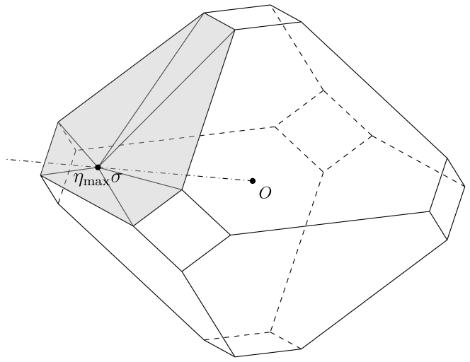
Figure 3: Geometric illustration of how to determine a minimal set of unitaries to prepare a target operator $\sigma$ with optimal efficiency.

We can further establish a strategy of optimal experimental design for state transfer under mixed unitary channels, which achieves best transfer efficiency and meanwhile minimizes the number of unitary experiments required. More precisely, we hope to find a minimal set of unitaries $U_{1},...,U_{K}$ to optimize

$$\min_{K}\max_{U_{1},...,U_{K}} \quad\eta,$$

such that $$\quad\sum\limits_{k=1}^{K}{\mu_{k}U_{k}\rho U^{\dagger}_{k}}=\eta\sigma.$$ (5)

It is evident that this problem can be reduced to the case when $\rho$ and $\sigma$ are both diagonal. For such a reduced case, we now show that the solution is provided by a set of diagonal permutation operations. Let $\mathcal{R}$ denote the set $\left\{\eta\sigma:\eta\geq 0\right\}$, it is a ray starting from the center $\bm{1}/N$. As the vector of diagonal elements of the operators that are accessible from $\rho$ under mixed unitary channels is bounded by the permutohedron $\mathcal{P}_{N}(\bm{\lambda}^{\rho})$, so the intersection point between $\mathcal{R}$ and $\mathcal{P}_{N}(\bm{\lambda}^{\rho})$ is $\eta_{\max}\sigma$. This point lies on a certain face of $\mathcal{P}_{N}(\bm{\lambda}^{\rho})$, and suppose the vertices of that face are $\left\{P_{s_{i}}\bm{\lambda}^{\rho}:{s_{i}\in S}\right\}$, with $S\subset\left\{1,...,N!\right\}$ being an index set. Now it is easy to see that, the minimal number of unitaries for preparing $\eta_{\max}\sigma$ equals to $\operatorname{rank}(\eta_{\max}\sigma,P_{s_{1}}\bm{\lambda}^{\rho},P_{s_{2}}\bm{\lambda}^{\rho},...)$, and one can set up a system of linear equations to solve out the necessary permutation operations and the corresponding weights. This procedure is geometrically illustrated with an example in Fig. 3. It is to be noted that, Eq. (5) has many optimal solutions. In practice, to choose a mixed unitary channel from the optimal ones, needless to say, we prefer those diagonal permutation operations that are easier to implement in experiment.

II.3 Markovian channel under coherent control

In open quantum system engineering, Markovian channels are often employed to directly describe the underlying noisy physical processes governing the evolution. They are frequently used to model realistic experimental set-ups, especially in NMR systems under relaxation, quantum optics, and condensed-matter physics, where external noises must invariably be accounted for. If the correlation time of the environmental noises is much faster than that of the system, then to a good approximation the underlying physical processes are forgetful. This is the Markovian assumption. Mathematically, a Markovian master equation generates a one-parameter (time $t$) semi-group of CPTP (completely positive and trace preserving) maps. Under the Markovian assumption, the system evolution under the joint action of coherent control and noise perturbation can be described by the Lindblad equation Lindblad (1976); Breuer and Petruccione (2002)

$$\dot{\rho}=\mathcal{\hat{L}}\rho=-i\left[{{H_{S}}+{H_{C}}(t),\rho}\right]+\hat{\mathcal{R}}\rho,$$ (6)

where we have set the Planck constant $\hbar$ to be 1, $H_{S}$ is the system Hamiltonian, $H_{C}(t)$ is the time-dependent external control Hamiltonian, and $\hat{\mathcal{R}}$ is a superoperator of Lindblad type $\mathcal{\hat{R}}\rho=\sum_{\alpha}{\gamma_{\alpha}(2L_{\alpha}\rho L^{\dagger}_{\alpha}-L^{\dagger}_{\alpha}L_{\alpha}\rho-\rho L^{\dagger}_{\alpha}L_{\alpha})}$ with $L_{\alpha}$ being Lindblad operators representing non-unitary effects.

The Lindblad equation leads to a dynamical map $\mathcal{\hat{E}}$ which steers an initial state $\rho(0)$ to another state $\rho(t)$ at time $t$. Because $\mathcal{\hat{E}}$ is non-unitary, it is possible to make an exact state transfer $\mathcal{\hat{E}}:\rho\to\eta\sigma$, where $\sigma$ is the target operator. Apparently, the bound for $\eta$ depends on the properties of $\mathcal{\hat{R}}$. Since decoherence is one of the main obstacles in developing quantum information technology, estimating the impact of decoherence on state transfer efficiency is hence of great importance to evaluate the realistic performance. Unfortunately, seeking the limit for reachability that is applicable for a general open Markovian quantum system driven by decoherence process and coherent controls remains an unsolved problem. Only partial results exist. For example, the reachable set on the states of a single qubit under dissipation has been established in Refs. Yuan (2010, 2012). Also, enormous efforts have been made to generalize these results to higher dimensional systems Altafini (2003, 2004); Kurniawan et al. (2012); Rooney (2012); Li et al. (2016a); Rooney and Bloch (2018).

Markovian channel under coherent control is interesting for the following reasons. First, a controlled relaxing system leads to a strictly contractive quantum channel, meaning that for any fixed pair of initial states, their distance is a strictly decreasing function of time Rivas and Huelga (2012). Therefore, it is possible to develop periodic control schemes which promise the capability of driving the system asymptotically to some periodic steady state. Such a property ensures that the target state can be periodically retained. The other reason, somehow surprisingly, is that open system control may exhibit advantages in some circumstances, e.g., in heat-bath algorithmic cooling protocol, higher purification efficiency can be achieved by utilizing relaxation Ryan et al. (2008). Therefore, it is worth studying the conditions on which Markovian channels could offer enhancement of state transfer efficiency beyond the universal bound on spin dynamics. In our subsequent experimental part, we will demonstrate these merits with concrete examples.

III NMR Based Control Models

For a given physical system, recognizing the available control means and establishing proper control models are crucial for developing practical control methods. A control model involves three necessary ingredients: system dynamics, admissible controls and control performance. This section gives a brief description of the relevant control models that are useful in liquid NMR experiments.

Coherent control. There have been developed substantial control techniques in NMR spin systems; for a survey, see Ref. Vandersypen and Chuang (2005). The most frequently used control technique in NMR spectroscopy is to excite the nuclear spins with radio-frequency (RF) pulses. Let the natural Hamiltonian describing the coupled spins be denoted by $H_{S}$, let the time-dependent control Hamiltonian representing RF fields be denoted by $H_{C}(t)$, then the system state evolves according to the Liouville-von-Neumann equation

$$\dot{\rho}(t)=-i[{H_{S}}+{H_{C}}(t),\rho(t)].$$ (7)

This is a closed quantum system control model, where RF excitation is coherent and enables universal control.

Gradient field control. Incoherent controls are often implemented by applying gradient fields, which exploit the different sensitivity of coherence orders to magnetic field inhomogeneity. Pulsed magnetic field gradients are mainly used for destructing the transverse magnetization of the sample, for on occasions only longitudinal magnetization is desired at some step of the evolution pathway. Here, the longitudinal direction, denoted as the $\hat{z}$ axis, is along the large static magnetic field $B_{0}$. A gradient field along $\hat{z}$ can introduce a dephasing for the coherences associated with different spatial locations along the sample.

Consider the most simple case that, a constant inhomogeneous field $B^{\prime}(z)=gz$ in $\hat{z}$ direction is applied, where $z\in[-L,L]$ with $2L$ being the length of the sample region, and $g$ is the field gradient, so that the total field is $\bm{B}(z)=B_{0}{\hat{z}}+B^{\prime}(z){\hat{z}}$. The system Hamiltonian is then $H_{z}=\gamma(B_{0}+gz)\sigma_{z}/2$, here $\gamma$ is the gyromagnetic ratio. Under this Hamiltonian, the $\nu$-th coherence terms $\sigma_{\nu}$ will evolve into

$$\sigma^{p}(t) =\exp(-iH_{z}t)\sigma_{\nu}(0)\exp(iH_{z}t)$$

$$=\exp[-i\nu\gamma(B_{0}+gz)t]\sigma_{\nu}(0).$$

Taking the ensemble average of the above expression with respect to $z$, there is

$$\left\langle\sigma_{\nu}(t)\right\rangle=\int_{z}{{U_{z}}(t){\sigma_{\nu}}(0)U_{z}^{\dagger}(t)}dz=\sigma_{\nu}(0)\delta_{\nu,0}.$$ (8)

Therefore, except for zero-th order quantum coherences, all other non-diagonal elements of the density matrix will be eliminated. In other words, one can regard the macroscopic sample as being constituted by a set of sub-ensembles each one represented by a density matrix with the same distribution of populations, but with off-diagonal elements out of phase. Averaging over these sub-ensemble is then equivalent to that the system undergoes a mixed unitary channel.

Figure 4: Illustration of the non-unitary evolution under gradient field control. Because the dephasing is proportional to the gradient strength, the coherences vary from 0 to $2\pi$ along the sample.

Phase cycling. An alternative to gradient field control that can be used in many instances to discriminate against particular coherence pathways is phase cycling. In many pulse NMR techniques, some sort of phase cycling procedure serves as an integral part of the experiment, e.g., NOESY Levitt (2008). Phase cycling can be used for the reduction or even elimination of unwanted signal components, giving rise to signal distortions. It is a method that lies at the very heart of almost every NMR experiment, especially playing a critical role in 2D NMR.

Phase cycling refers to the repetition of a pulse sequence a number of times, with varying the phases of the RF pulses, the receiver, and digitizer in a predetermined pattern. With judiciously changing the phases from experiment to experiment, the final signals are averaged such that the desired component is retained while undesired routes are rejected. To illustrate the idea, consider a simple phase cycling scheme aiming to select wanted coherences. In the $k$th experiment, we apply a collective rotation of the spins with angle $\theta_{k}$ about the $\hat{z}$ axis, then in the final averaged signal, any $\nu$ coherence term $\sigma_{\nu}$ will be turned into

$${\sigma_{\nu}}\to{\sigma_{\nu}}\sum\limits_{k}{{e^{-i{\nu\theta_{k}}}}}.$$ (9)

Through a special design of the phases $\theta_{k}$, the desired coherence terms can be enhanced, while the undesired ones are canceled by intendedly setting $\sum\nolimits_{k}{{e^{-i\nu\theta_{k}}}}=0$, when adding up the signals. Generally, phase cycling schemes can be rather complex. It is easy to see that the influence of a phase cycling to quantum states can be directly represented as a mixed unitary channel. Therefore, the phase cycling technique can not exceed the universal bound on spin dynamics.

Control of relaxation process. In NMR, relaxation is always present, and affects the system’s state in an irreversible way. The formalism of liquid NMR relaxation theory has been well developed. We refer the reader to standard textbooks such as Refs. Levitt (2008); Kowalewski and Mäler (2018) for theoretical details. Under appropriate assumptions, the relaxation dynamics of a liquid-state NMR spin system can be described by the Lindblad equation (6). A detailed analysis of the state transfer problem under coherently controlled relaxation equation was given in Ref. Li et al. (2016a), where it was found that when relaxation is properly utilized, it is possible to surpass the universal bound on spin dynamics. Whether or not this possibility can happen is dependent on the relaxation parameters in the evolution equation.

IV Applications to PPS Preparation

In this section, we investigate the application of quantum control models to state engineering tasks in liquid-state NMR quantum information processing. Specifically, we focus on the problem of pseudopure state (PPS) preparation Cory et al. (1998); Gershenfeld and Chuang (1997); Knill et al. (1998). Pseudopure states are used as the initial states for quantum computing. From these states, one can prepare other quantum states such as Bell states via quantum circuits.

IV.1 PPS preparation problem

One important motivation of studying the PPS preparation problem is that, the low polarization of NMR spin ensemble at room temperature makes it rather difficult to get a genuine pure state. Therefore, PPS was introduced as a substitute. It offers a faithful representation for the transformations of pure states. Especially, it turns out that the concept of PPS is suitable for benchmark experiments.

We consider creating pseudopure states on a spin system with weakly coupled $n$ spin-1/2 nuclei. We want to prepare the following form of mixed state

$$\rho_{\text{pps}}=(1-\eta)\frac{I^{\otimes n}}{2^{n}}+\eta\left|0^{\otimes n}\right\rangle\left\langle 0^{\otimes n}\right|,$$ (10)

where $I$ is the $2\times 2$ identity matrix, and $\eta$ is referred to as the effective purity of the state. Let $X,Y,Z$ denote the three Pauli operators $\sigma_{x},\sigma_{y},\sigma_{z}$ respectively, then PPS can also be written as

$${\rho_{\text{pps}}}= {}\frac{I^{\otimes n}}{2^{n}}+\frac{\eta}{2^{n}}(Z_{1}+\ldots+Z_{n}+Z_{1}Z_{2}+\ldots+$$

$${}Z_{n}Z_{1}+\ldots+Z_{1}Z_{2}\cdots Z_{n}).$$ (11)

Effective purity is an important parameter since it determines the intensity of the observed signals. NMR suffers from inherently low sensitivity, and it is desirable to improve the spectral signal-to-noise ratio as much as possible.

The initialization process usually starts with the system’s thermal equilibrium state $\rho_{eq}$, which satisfies the Boltzmann distribution and takes the following form if high temperature approximation is used

$${\rho_{\text{eq}}}-\frac{I^{\otimes n}}{2^{n}}\propto\epsilon\sum\limits_{i=1}^{n}{{\gamma_{i}}{Z_{i}}},$$ (12)

where $\gamma_{i}$ is the gyromagnetic ratio of the $i$-th nucleus and the factor $\epsilon\simeq{10^{-5}}$ is related to the thermal polarization of the system. The polarization is actually rather low, which is responsible for the difficulty of producing pure states.

The PPS task, i.e., $\rho_{\text{eq}}\to\rho_{\text{pps}}$, can not be done merely with unitary operations, as $\rho_{\text{eq}}$ and $\rho_{\text{pps}}$ have different spectra. Methods of PPS preparation often involve different ways of realizing non-unitary operations Knill et al. (2000); Sakaguchi et al. (2000); Jones (2001), such as exertion of gradient fields, phase cycling or even relaxation channels. To simplify the discussion of the PPS preparation problem, we use a heteronuclear system (¹H and ¹³C) as an example. In spite of this, note that in principle the approaches presented in the following can be generalized to any number of qubits. The diagonal part of the state of our two-spin system can always be decomposed as $II/4+x_{1}Z_{1}+x_{2}Z_{2}+x_{3}Z_{1}Z_{2}$, which we denote as a vector $(x_{1},x_{2},x_{3})$. For example, let $\epsilon$ denote the polarization magnitude of the ¹³C spin, then the equilibrium state $\rho_{\text{eq}}$ is written as $(\epsilon,4\epsilon,0)$. The diagonal permutations of $\rho_{\text{eq}}$ are all shown in Fig. 5. In the language of polarization transfer, our task amounts to the conversion between the operators $\rho=\epsilon(Z_{1}+4Z_{2})$ and $\sigma=-II/4+\left|00\right\rangle\left\langle 00\right|$. As discussed in Sec. II, the universal bound on spin dynamics suggests that the highest unitary transfer efficiency achievable is

$$\eta_{\max}=\frac{\bm{\lambda}^{\rho}_{\downarrow}\cdot\bm{\lambda}^{\sigma}_{\downarrow}}{\bm{\lambda}^{\sigma}_{\downarrow}\cdot\bm{\lambda}^{\sigma}_{\downarrow}}=\frac{20}{3}\epsilon,$$ (13)

no matter we use techniques of gradient fields or phase cycling or both. The unitary bound or mixed-unitary bound is geometrically illustrated in Fig. 5.

Figure 5: The permutohedron constructed by taking the convex hull of all 4-vectors from the $4!=24$ diagonal permutations of $\rho_{\text{eq}}$.

IV.2 Methods for PPS preparation

Here we present some examples of methods for PPS preparation, with major concern on their transfer efficiencies. In the following, method (1) is an average of multiple unitary control experiments; methods (2) spatial averaging method, (3) line selective method, and (4) controlled-transfer gate method all utilize gradient fields to realize necessary non-unitary controls. They can achieve transfer efficiency at most $\eta_{\max}$ in Eq. (13). We also describe two novel PPS preparation methods (4) and (5), which take the relaxation effects as the required non-unitary resource and remarkably, both allow to surpass the limit $\eta_{\max}$. We use a concrete two-spin system as a simple application example to show the transfer efficiencies for these preparation methods. The system is ¹³C-labeled chloroform ¹³CHCl₃, which consists of a carbon spin and a proton spin. We use $J$ to denote the coupling between the two spins.

(1) Time averaging (TA) method. This method Knill et al. (1998) simply involves averaging over three unitary experiments, i.e.,

$$\begin{rcases}\rho_{\text{eq}}\to Z_{1}+4Z_{2}&\\ \rho_{\text{eq}}\to Z_{2}+4Z_{1}Z_{2}&\\ \rho_{\text{eq}}\to 4Z_{1}+Z_{1}Z_{2}&\end{rcases}\to\rho_{\text{pps}}=\frac{5}{3}(Z_{1}+Z_{2}+Z_{1}Z_{2}).$$

From Fig. 5, we know that at least three unitary experiments are needed to get PPS, and there actually exist many choices for these unitaries to achieve the optimal bound $6.67\epsilon$.

(2) Spatial averaging (SA) method. SA Cory et al. (1998) exploits a series of RF pulses sequentially and repeated field gradient pulses, equalizing gradually the populations of all energy levels except one.

For the CH-two-spin system, we apply the pulse sequence $[R_{x}^{\text{C,H}}(90^{\circ})-1/(4J)-R_{y}^{\text{C,H}}(90^{\circ})-1/(4J)-R_{-x}^{\text{C,H}}(90^{\circ})-\operatorname{G}_{z}-R_{x}^{\text{C,H}}(45^{\circ})-1/(2J)-R_{-y}^{\text{C,H}}(30^{\circ})-\operatorname{G}_{z}]$, where $R_{\pm x(\pm y)}^{\text{C,H}}(\theta)$ denotes a hard pulse rotating the ${}^{1}\text{H}$ and ${}^{13}\text{C}$ nuclei about $\pm x(\pm y)$ axis with $\theta$ degree and $\operatorname{G}_{z}$ denotes a gradient pulse along $\hat{z}$ direction to eliminate off-diagonal elements of the state. This transforms the operator $ZI+4IZ$ to $5\sqrt{3}/\sqrt{2}(-II/4+\left|00\right\rangle\left\langle 00\right|)$. Therefore, the transfer efficiency is $\eta=5\sqrt{3}/\sqrt{2}\epsilon\approx 6.12\epsilon$. SA does not achieve the universal bound on spin dynamics, since there involves in a number of gradient pulses, each one causing polarization lost and hence reducing the final spectral signal.

(3) Line selective (LS) method. In this method, one first coherently drive the system from $\rho_{\text{eq}}$ to a state satisfying that the diagonal population distribution of which takes the same form as that of $\rho_{\text{pps}}$, and then applies a gradient pulse to remove the off-diagonal elements while keeping the diagonal elements unchanged. Line-selective pulses are designed to implement the wanted population flips between the target energy levels. By leaving the ground state untouched and averaging the other states, LS method can acquire the general bound of spin dynamics Madi et al. (1998); Peng et al. (2001); Zheng et al. (2018).

Generally, the LS method requires to find a set of parameters $\{{x_{\alpha}}\}_{\alpha={1,\ldots,2^{n-1}}}$, so that the following unitary operator $U_{d}=e^{-i\sum\nolimits_{\alpha}{{x_{\alpha}}I_{x}^{(\alpha+1,\alpha+2)}}}$, where $I_{x}^{(\alpha+1,\alpha+2)}$ is the single quantum transition operator between levels $\alpha+1$ and $\alpha+2$, can fulfill the equation

$$\operatorname{diag}\left[{U_{d}}\left({\rho_{\text{eq}}}-\frac{{{I^{\otimes n}}}}{{{2^{n}}}}\right)U_{d}^{\dagger}\right]$$

$$={} {\eta_{\max}}\times\operatorname{diag}\left[-\frac{{{I^{\otimes n}}}}{{{2^{n}}}}+\left|{{0^{\otimes n}}}\right\rangle\left\langle{{0^{\otimes n}}}\right|\right].$$

For example, in the C,H-two-spin system, the operator

$${U_{d}}=\exp\left\{{-i\left({{x_{1}}I_{x}^{(2,3)}+{x_{2}}I_{x}^{(3,4)}}\right)}\right\},$$

with ${x_{1}}={31.78^{\circ}}$ and ${x_{2}}={46.50^{\circ}}$, can be used to create PPS with the highest unitary transfer efficiency $\eta\approx 6.67\epsilon$. Here $I_{x}^{(2,3)}=IX-ZX$ and $I_{x}^{(3,4)}=XI-XZ$ are quantum transition operators related to the transitions $\left|{10}\right\rangle\leftrightarrow\left|{11}\right\rangle$ and $\left|{01}\right\rangle\leftrightarrow\left|{11}\right\rangle$, respectively. For more complex systems, the parameters $\{{x_{\alpha}}\}$ can be obtained by numerical searching algorithms.

(4) Controlled-transfer gate (CTG) method. Similar to the LS method, the CTG method allows maximal unitary transfer efficiency also via the idea of averaging the populations of states other than the ground state. It utilizes the so called controlled-transfer gate, which includes two controlled-rotation gates and one gradient field, to realize the redistribution process (Fig. 6) Kawamura et al. (2010). The controlled-rotation axes are in the $xy$ plane and the effectiveness of the method does not depend on the specific choice of the axes. Rotation angles should be specially designed according to the initial populations of the state. Set rotation angles as $\pi/2$ and repeat the CTGs several times with long enough intervals, the state can be asymptotically driven toward a PPS whatever the initial state is. For the C,H-two-spin system, one CTG is enough to achieve PPS transfer efficiency $\eta\approx 6.67\epsilon$ from the thermal equilibrium state by choosing ${\theta_{1}}=99.59^{\circ}$ and ${\theta_{2}}=90^{\circ}$.

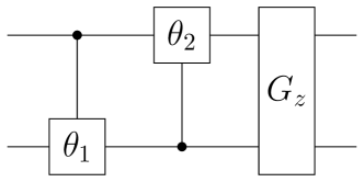
Figure 6: The pulse sequence for two-qubit PPS preparation with controlled-transfer gate.

Figure 7: Experimental demonstration of pseudopure states prepared using previous approaches and our new approaches. From left to right, (a-g) are spectra obtained by applying readout pulses to the thermal equilibrium state (a), PPS prepared by spatial averaging method (b), by line selective method (c), by controlled-transfer gate method (d), by periodic control (e), and by line selective saturation method (f), respectively. The small signal visible at the center of the 1H spectrum arises from an impurity (unlabeled formate). All spectra are plotted on the same vertical scale.

(5) Periodic control (PC) method. In Ref. Li et al. (2016a) it was shown that a simple periodic sequence described by ${\left[{V-\tau}\right]_{m}}$ is capable of preparing PPS, where $V$ is a unitary operation, $\tau$ represents free relaxation, and $m$ means the number of times that the sequence is repeated. Under this sequence, the total evolution superoperator is $\mathcal{\hat{E}}={(\mathcal{\hat{E}}_{V}\mathcal{\hat{E}}_{\tau})^{m}}$. Our goal is to construct such a sequence so that the desired state $\rho_{\text{pps}}$ is the corresponding fixed point: $\mathcal{\hat{E}}\rho_{\text{pps}}=\rho_{\text{pps}}$.

During the free evolution periods, the NMR system is under both longitudinal and transverse relaxation, with their respective characteristic time denoted by ${T_{1}}$ and ${T_{2}}$. The longitudinal relaxation tends to steer the diagonal terms of the state to the equilibrium distribution, and the transverse relaxation destructs all non-diagonal terms. It is straightforward to conceive a cyclic permutation process of the diagonal terms to realize PPS preparation. For example, $V$ can be chosen to be

$$V=\left[{\begin{array}[]{*{20}{c}}1&{}\hfil&{}\hfil&{}\hfil&{}\hfil\\ {}\hfil&{}\hfil&{}\hfil&{}\hfil&1\\ {}\hfil&1&{}\hfil&{}\hfil&{}\hfil\\ {}\hfil&{}\hfil&\ddots&{}\hfil&{}\hfil\\ {}\hfil&{}\hfil&{}\hfil&1&{}\hfil\\ \end{array}}\right].$$

It is easy to see that $V$ is to perform a permutation of the diagonal elements except the first element ${\rho_{11}}$, and it satisfies ${V^{({2^{n}}-1)}}=\text{identity}$. If no relaxation is involved, the permutation operation does nothing but changing the order of the diagonal elements. However, if there are relaxation processes, relaxation would slowly and continuously change the diagonal elements (except $\rho_{11}$) until all of them are equal. In other words, PPS is a fixed point of $V$ and becomes achievable due to the non-unitary modulation by relaxation. Note that, unlike in LS method and CTG method, the introducing of a longitudinal relaxation process may increase $\rho_{11}$, while coherent controls can not. Therefore, PC method provides us a route to surpass the highest transfer efficiency in previous methods.

For the C,H-two-spin system, $V$ can be easily decomposed into elementary gates as $[R^{\text{H}}_{y}(90^{\circ})-1/(2J)-R^{\text{H}}_{x}(90^{\circ})-R^{\text{C}}_{y}(90^{\circ})-1/(2J)-R^{\text{C}}_{x}(90^{\circ})]$.

(6) Line selective saturation (LSS) method. It is a common NMR technique to average two energy populations by continuously exposing them to a resonant RF wave. As an extension of this technique, here we put forward a new approach to prepare PPS via saturating the involved energy populations. A shaped RF wave is tailored to simultaneously excite energy level inversions between any two energy states excluding the ground state. In the case that NMR spectral lines can be well resolved, low power square waves of long durations can accomplish this task. The irradiation should keep on until the saturation condition is achieved. The time scale of this process is often tens of seconds, longer than the longitudinal relaxation time $T_{1}$. During the irradiation, the generated off-diagonal terms are gradually eliminated by transverse relaxation. Similarly with the PC method, the longitudinal relaxation may lead to a growth of ground state population $\rho_{11}$ due to cross-relaxation. This makes it possible to surpass the bound of the unitary transfer efficiency.

Method	SA	LS	CTG	PC	LSS
Transfer efficiency	$5.60\epsilon$	$6.21\epsilon$	$6.60\epsilon$	$6.83\epsilon$	$6.88\epsilon$

Table 1: Experimental comparison of transfer efficiencies among different PPS approaches.

IV.3 Experimental results

Our experiments were carried out on a Bruker AVANCE spectrometer with a nominal ¹H frequency of 600 MHz at room temperature. The experimental system is the two-qubit heteronuclear spin system (¹H and ¹³C) provided by ¹³C enriched chloroform ($\rm CHC{l_{3}}$) dissolved in deuterated acetone. ¹³C nucleus is labeled as qubit 1 and ¹H nucleus is labeled as qubit 2. Both nuclear spins were placed on resonance in their respective rotating frames, so the effective system Hamiltonian contains only a scalar coupling term $H_{S}=\pi JZ_{1}Z_{2}/2$ with $J=214.5$ Hz.

We have realized PPS preparation from the aforementioned different methods. The creation of PPS requires both coherent and incoherent controls. Incoherent controls were implemented either by applying gradient field pulses of 1 ms duration or via free relaxation evolution. For the SA method, we only need hard pulse rotations as well as free evolution in between. For the LS method and CTG method, we engineered the required unitary operations as shaped pulses which are optimized by the gradient ascent pulse engineering (GRAPE) algorithm Khaneja et al. (2005). The shaped pulses were functionalized to equalize the populations of all energy levels except the first one, namely to leave the ground state untouched. For the PC method, the period $\tau$ of free relaxation evolution of each cycle was set to $300$ ms. Then PPS was reached after $m=60$ loops. For the LSS method, the line selective saturation operation was realized by two low power rectangular pulses, whose frequencies are set to be resonant with the energy level transitions $\left|{10}\right\rangle\leftrightarrow\left|{11}\right\rangle$ and $\left|{01}\right\rangle\leftrightarrow\left|{11}\right\rangle$, respectively. One can also choose to use pulse shapes other than a rectangle one, such as a selective soft Gaussian shape. The two excitation pulses were simultaneously applied, one to the ¹³C channel and the other to the ¹H channel. After continuous irradiation over 3 seconds, the populations of the three energy eigenlevels $\left|{10}\right\rangle$, $\left|{01}\right\rangle$, and $\left|{11}\right\rangle$ were averaged, and then we got a PPS.

Figure 7 shows the experimental NMR spectra and Tab. 1 shows the comparison between the experimental transfer efficiencies achieved from different PPS approaches. One can see that relaxation assisted methods can outperform mixed unitary channels. The deviations between theoretical expectations and experimental results mainly arise from the imperfections of RF pulses.

V Application to Labelled-PPS Preparation

V.1 Labelled-PPS

Since that in many circumstances PPS is still challenging to prepare, one uses labelled-PPS as a substitute, which takes the form:

$$\rho_{\text{lpps}}=Z\otimes|0\rangle\langle 0|^{\otimes(n-1)}.$$ (14)

Thus in an $n$-qubit labelled-PPS, there are $n-1$ qubits being initialized at $|0\rangle\langle 0|$. Preparing labelled PPS can be less resource demanding than preparing PPS. Indeed, this has been experimentally realized in a 3-qubit system Knill et al. (2000) and later even in a 12-qubit system Negrevergne et al. (2006).

V.2 Conventional method

The standard method for preparing labelled-PPS employs phase cycling. The process can be summarized as follows

$$\rho_{\text{eq}} \to\rho_{0}=Z{I^{\otimes(n-1)}}$$

$$\to\rho_{\text{ad}}={X^{\otimes n}}$$

$$\to\rho_{\text{mc}}=\frac{1}{2^{n}}(X+iY)^{\otimes n}+\frac{1}{2^{n}}(X-iY)^{\otimes n}$$

$$\to\rho_{\text{lpps}}=Z\otimes|0\rangle\langle 0|^{\otimes(n-1)}.$$ (15)

The first step can be done through gradient fields. The intermediate state $\rho_{\text{ad}}$ is composed of all anti-diagonal terms. So the coherence orders contained in $\rho_{\text{ad}}$ are $-n,-n+2,\ldots,n$. The maximal coherence state $\rho_{\text{mc}}$ is the deviation density matrix for the cat state, i.e., the $n$-coherence $|{{0^{\otimes n}}}\rangle\langle{1^{\otimes n}}|+|{{1^{\otimes n}}}\rangle\langle{0^{\otimes n}}|$. In the final step, the maximal coherence is turned to the labelled-PPS $\rho_{\text{lpps}}$ via a decoding procedure.

Figure 8: Experimental results of labelled-PPS preparation using conventional phase cycling method and our optimal strategy. (a) Full NMR equilibrium spectrum. where the chemical shifts (in Hz) of C₁, C₂ and C₃ nuclei are marked. (b,c) C₂ NMR spectra for labelled-PPS obtained by the phase cycling method (b) and by our optimal strategy (c). The middle three spectra in (b) and two spectra in (c) are obtained from implementing each unitary operation of the mixed unitary channel described in the main text. The bottom spectra in (b) and (c) are thermal equilibrium spectra of C₂ nucleus, and the top ones are the spectra of labelled-PPS, which are obtained by averaging the middle spectra.

The key step of the above method is to make the transform from $\rho_{\text{ad}}$ to $\rho_{\text{mc}}$. To accomplish this task, phase cycling is adopted to eliminate all the coherences whose order not equal to $n$ or $-n$. Concretely, we perform $K$ experiments, where in the $k$th experiment, we rotate each qubit by a phase $\theta_{k}$ about the $z$-axis, that is, we apply the following operation

$$U_{k}=\exp(-i\theta_{k}\sum_{j=1}^{n}Z_{j}/2).$$

Let $\sigma_{\nu}$ denote a $\nu$-coherence ($-n\leq\nu\leq n$), it acquires a phase $\nu\theta_{k}$ under $U_{k}$. The imposed phases thus label different orders of coherences. We discriminate two different cases.

(1) If $n$ is odd, implying that no zero-coherence exists in $\rho_{\text{ad}}$, then we set $K=n$ and $\theta_{k}=2\pi k/n$. We average the results of the $K$ experiments. One can check that, for a $\nu$-coherence $\sigma_{\nu}$, there is

$$\sigma_{\nu}\to\frac{1}{K}\sum_{k=1}^{K}e^{-i\nu\theta_{k}}\sigma_{\nu}= \sigma_{\nu}, \nu=\pm n$$ if ;

$$\sigma_{\nu}\to\frac{1}{K}\sum_{k=1}^{K}e^{-i\nu\theta_{k}}\sigma_{\nu}= 0,$$ otherwise.

(2) if $n$ is even, implying that there exist zero-coherences in $\rho_{\text{ad}}$, then we set $K=2n$ and $\theta_{k}=2\pi k/(2n)$. The results of the $K$ experiments are treated as such, the $k$th experimental result is added when $k$ is even and subtracted when $k$ is odd

$$\sigma_{\nu}\to\frac{1}{K}\sum_{k=1}^{K}(-1)^{k}e^{-i\nu\theta_{k}}\sigma_{\nu}= \sigma_{\nu}, \nu=\pm n$$ if ;

$$\sigma_{\nu}\to\frac{1}{K}\sum_{k=1}^{K}(-1)^{k}e^{-i\nu\theta_{k}}\sigma_{\nu}= 0,$$ otherwise.

Therefore, for these two cases, the above designed phase cycling preserves exclusively the maximal order coherences. The final signal can only originate from the $n$-coherences in $\rho_{\text{ad}}$. To summarize, the number of experiments need to be performed in this labelled-PPS preparation method is $n$ when $n$ is odd, and is $2n$ when $n$ is even.

V.3 Our optimal strategy

Here, we show that, actually just two experiments suffice to get the labelled-PPS. This is based on optimal experimental design under mixed unitary channels, which has been developed in Sec. II.2. One optimal solution is given as below

$$\frac{1}{2}\left(Z{I^{\otimes(n-1)}}+U\cdot Z{I^{\otimes(n-1)}}\cdot{U^{\dagger}}\right)=Z\otimes|0\rangle\langle 0|^{\otimes(n-1)},$$

where

$$U=\left[{\begin{array}[]{*{20}{c}}{\rm{1}}&{}\hfil&{}\hfil&{}\hfil\\ {}\hfil&{}\hfil&{}\hfil&1\\ {}\hfil&{}\hfil&{\mathinner{\mkern 2.0mu\raise 1.0pt\hbox{.}\mkern 2.0mu\raise 4.0pt\hbox{.}\mkern 2.0mu\raise 7.0pt\hbox{.}\mkern 1.0mu}}&{}\hfil\\ {}\hfil&1&{}\hfil&{}\hfil\\ \end{array}}\right].$$

So in the first experiment, we apply an identity operation, i.e., do nothing. In the second experiment, we apply the above operation $U$. Then we get labelled-PPS of optimal transfer efficiency. There exist substantially many optimal preparation strategies, which are essentially equivalent due to symmetry.

V.4 Experimental results

We carried out labelled-PPS preparation on a three-qubit system. The system is provided by a ¹³C-labeled alanine dissolved in deuterated acetone. The sample consists of three ¹³C nuclei, which are labelled as C₁ (qubit 1), C₂ (qubit 2) and C₃ (qubit 3), respectively. Figure 8(a) gives the thermal equilibrium spectrum of the sample. The mutual couplings between the spins are $J_{12}=53.97$ Hz, $J_{23}=34.9$ Hz and $J_{13}=-1.31$ Hz. Observation is made on C₂ because all the couplings are adequately resolved.

Conventional method. We start from the state $Z_{2}$, which can be readily obtained by first rotating the polarizations of C₁ and C₃ into the transverse plane, and then applying a gradient pulse. Then, the gate sequence $[R_{y}^{2}({90^{\circ}})-{e^{-i\pi{Z_{1}}{Z_{2}}/4}}-R_{y}^{\rm{1}}({90^{\circ}})-{e^{-i\pi{Z_{1}}{Z_{3}}/4}}-R_{y}^{\rm{3}}({90^{\circ}})]$ can be used to make the transform $Z_{2}\to Y_{1}Y_{2}X_{3}$. However, it is hard to find a simple pulse sequence to implement the operation $e^{-i\pi{Z_{1}}{Z_{3}}/4}$ within a duration much shorter than the transverse relaxation time, since the coupling $J_{13}$ is so weak. Therefore the gate sequence is integrated into a shaped pulse of 40 ms in the experiment, which is optimized by using the GRAPE technique. Next, we encode phases to the different coherences contained in $Y_{1}Y_{2}X_{3}$. As we have described previously, since the state $Y_{1}Y_{2}X_{3}$ contains just one-coherences and three-coherences, so three experiments are needed for the phase cycling procedure. The rotation angles of the three experiments are set to $0^{\circ}$, $120^{\circ}$ and $240^{\circ}$ respectively. After the encoding, another GRAPE pulse of 40 ms, corresponding to the sequence $[R_{-y}^{3}({90^{\circ}})-{e^{-i\pi{Z_{1}}{Z_{3}}/4}}-R_{-y}^{\rm{1}}({90^{\circ}})-{e^{-i\pi{Z_{1}}{Z_{2}}/4}}-R_{x}^{{\rm{1,3}}}({90^{\circ}})]$, was applied to decode the selected three-coherence into labelled-PPS, i.e., the state $|0\rangle\langle{0}|\otimes X\otimes|0\rangle\langle{0}|$.

Our method. The labelled-PPS can be prepared by a mixed unitary channel consisting of two unitary operations. We use the optimal strategy given in Sec. V.3. Each operation is realized by a GRAPE pulse of 40 ms. The experimental result is shown in Fig. 8, which confirms the validity of our optimal strategy for labelled-PPS preparation.

VI conclusions and discussions

Quantum state transfer represents one of the most fundamental problems in quantum engineering Dong and Petersen (2010); Brif et al. (2010) and has a wide range of applications Zhang et al. (2005); Qin et al. (2013, 2014); Li et al. (2017b); Chiu et al. (2018). Very often, it is important to ask what transfer efficiency can be achieved via available control means. In this work, we have examined this problem in detail. We show that the bound of unitarily convertible region, namely the optimal bound on spin dynamics, can not be extended through introducing mixed unitary channels, which are defined as probabilistic or weighted average of a set of unitary control experiments. Moreover, having prior knowledge of the optimal bound under mixed unitary channels, a minimal set of unitaries can be constructed to achieve the best transfer efficiency. This gives optimal experimental design strategy. We explore the application of state transfer bound theories to realistic state engineering tasks in liquid NMR systems. Specifically, both theoretical and experimental investigations are conducted on the PPS preparation problem. We show that larger transfer efficiency can be achieved, with the aid of relaxation effects, which are usually considered as playing negative roles in quantum system control.

Applying the optimal strategy of designing mixed unitary channels to NMR spectroscopy is a subject worthy of study. Some NMR techniques, such as COSY and INADEQUATE experiments Levitt (2008), whose cores are phase cycling, may gain improvements of experimental efficiency if optimal strategy can be constructed. As to the theoretical aspect, our present study can be regarded as a step in exploring the bound of state transfer under general quantum channels. Future work will consider the extension of the theory to other non-unitary control models, such as quantum measurement Buffoni et al. (2019), reservoir engineering Verstraete et al. (2009); Vuglar et al. (2018) and hybrid quantum-classical control Li et al. (2017a); Yang et al. (2017), which have already attracted great interests in recent quantum information processing experiments.

VII Acknowledgments

W. Z., H. W, J. L., T. X., and D. L. are supported by the National Natural Science Foundation of China (Grants No. 11605153, No. 11605005, No. 11875159 and No. U1801661), Science, Technology and Innovation Commission of Shenzhen Municipality (Grants No. ZDSYS20170303165926217 and No. JCYJ20170412152620376), Guangdong Innovative and Entrepreneurial Research Team Program (Grant No. 2016ZT06D348), the National Natural Science Foundation of Zhejiang province (Grants No. LQ19A050001).

References

- Dong and Petersen (2010) D. Dong and I. R. Petersen, IET Control Theory Appl. 4, 2651 (2010).
- Brif et al. (2010) C. Brif, R. Chakrabarti, and H. Rabitz, New J. Phys. 12, 075008 (2010).
- Levi et al. (2015) L. Levi, W. Skomorowski, L. Rybak, R. Kosloff, C. P. Koch, and Z. Amitay1, Phys. Rev. Lett. 114, 233003 (2015).
- Olson et al. (2016) J. Olson, Y. Cao, J. Romero, P. Johnson, P.-L. Dallaire-Demers, N. Sawaya, P. Narang, I. Kivlichan, M. Wasielewski, and A. Aspuru-Guzik, NSF Workshop Report arXiv:1706.05413 (2016).
- McDonald et al. (2018) M. McDonald, I. Majewska, C.-H. Lee, S. S. Kondov, B. H. McGuyer, R. Moszynski, and T. Zelevinsky, Phys. Rev. Lett. 120, 033201 (2018).
- Wang et al. (2011) X. Wang, S. Vinjanampathy, F. W. Strauch, and K. Jacobs, Phys. Rev. Lett. 107, 177204 (2011).
- Kosloff (2013) R. Kosloff, Entropy 15, 2100 (2013).
- Gelbwaser-Klimovsky et al. (2015) D. Gelbwaser-Klimovsky, W. Niedenzu, and G. Kurizki, Adv. Atom Mol. Opt. Phys. 64, 329 (2015).
- Pang and Jordan (2017) S. Pang and A. N. Jordan, Nat. Commun. 8, 14695 (2017).
- Poggiali et al. (2018) F. Poggiali, P. Cappellaro, and N. Fabbri, Phys. Rev. X 8, 021059 (2018).
- Vandersypen and Chuang (2005) L. M. K. Vandersypen and I. L. Chuang, Rev. Mod. Phys. 76, 1037 (2005).
- Altafini and Ticozzi (2012) C. Altafini and F. Ticozzi, IEEE Trans. Automat. Contr. 57, 1898 (2012).
- Werschnik and Gross (2007) J. Werschnik and E. K. U. Gross, J. Phys. B: At. Mol. Opt. Phys. 40, 175 (2007).
- Glaser et al. (2015) S. J. Glaser, U. Boscain, T. Calarco, C. P. Koch, W. Köckenberger, R. Kosloff, I. Kuprov, B. Luy, S. Schirmer, T. Schulte-Herbrüggen, D. Sugny, and F. K. Wilhelm, Eur. Phys. J. D 69, 279 (2015).
- Altafini (2003) C. Altafini, J. Math. Phys. 44, 2357 (2003).
- Verstraete et al. (2009) F. Verstraete, M. M.Wolf, and J. I. Cirac, Nat. Phys. 5, 633 (2009).
- Koch (2016) C. P. Koch, J. Phys.: Condens. Matter 28, 213001 (2016).
- Li et al. (2016a) J. Li, D. Lu, Z. Luo, R. Laflamme, X. Peng, and J. Du, Phys. Rev. A 94, 012312 (2016a).
- Ashhab and Nori (2010) S. Ashhab and F. Nori, Phys. Rev. A 82, 062103 (2010).
- Pechen et al. (2006) A. Pechen, N. Il’in, F. Shuang, and H. Rabitz, Phys. Rev. A 74, 052102 (2006).
- Rabitz et al. (2000) H. Rabitz, R. D. Vivie-Riedle, M. Motzkus, and K. Kompa, Science 288, 824 (2000).
- Lloyd and Viola (2001) S. Lloyd and L. Viola, Phys. Rev. A 65, 010101 (2001).
- Zhang et al. (2017) J. Zhang, Y. xi Liu, R.-B. Wu, K. Jacobs, and F. Nori, Physics Reports 679, 1 (2017).
- Li et al. (2017a) J. Li, X. Yang, X. Peng, and C.-P. Sun, Phys. Rev. Lett. 118, 150503 (2017a).
- Schirmer and Wang (2010) S. G. Schirmer and X. Wang, Phys. Rev. A 81, 062306 (2010).
- Poyatos et al. (1996) J. F. Poyatos, J. I. Cirac, and P. Zoller, Phys. Rev. Lett. 77, 4728 (1996).
- Roa et al. (2006) L. Roa, A. Delgado, M. L. L. de Guevara, and A. B. Klimov, Phys. Rev. A 73, 012322 (2006).
- Heinosaari and Ziman (2012) T. Heinosaari and M. Ziman, The Mathematical Language of Quantum Theory: From Uncertainty to Entanglement (Cambridge University Press, Cambridge, 2012).
- Sørensen (1990) O. W. Sørensen, J. Magn. Reson. 86, 435 (1990).
- Stoustrup et al. (1995) J. Stoustrup, O. Schedletzky, S. J. Glaser, C. Griesinger, N. C. Nielsen, and O. W. Sørensen, Phys. Rev. Lett. 74, 2921 (1995).
- Nielsen et al. (1995) N. C. Nielsen, T. Schulte-Herbrüggen, and O. W. Sørensen, Molecular Physics 85, 1205 (1995).
- Nielsen et al. (1996) N. C. Nielsen, H. Thøgersen, and O. W. Sørensen, J. Chem. Phys. 105, 3962 (1996).
- Hughes and Wimperis (1997) C. E. Hughes and S. Wimperis, J. Chem. Phys. 106, 2105 (1997).
- Untidt and Nielsen (2000) T. S. Untidt and N. C. Nielsen, J. Chem. Phys. 113, 8464 (2000).
- Khaneja et al. (2003) N. Khaneja, B. Luy, and S. J. Glaser, PNAS 100, 13162 (2003).
- Levitt (2016) M. H. Levitt, J. Magn. Reson. 262, 91 (2016).
- Li et al. (2016b) C.-K. Li, D. C. Pelejo, and K.-Z. Wang, Quantum Inf. Comput. 16, 845 (2016b).
- Cory et al. (1998) D. G. Cory, M. D. Price, and T. F. Havel, Physica D 120, 82 (1998).
- Gershenfeld and Chuang (1997) N. A. Gershenfeld and I. L. Chuang, Science 275, 350 (1997).
- Knill et al. (1998) E. Knill, I. Chuang, and R. Laflamme, Phys. Rev. A 57, 3348 (1998).
- Horn and Johnson (2013) R. A. Horn and C. R. Johnson, Matrix Analysis (Cambridge University Press, Cambridge, 2013).
- Kraus (1983) K. Kraus, States, Effects, and Operations: Fundamental Notions of Quantum Theory (Springer-Verlag, Berlin, 1983).
- Li and Poon (2011) C.-K. Li and Y.-T. Poon, Linear and Multilinear Algebra 59, 1159 (2011).
- Lindblad (1976) G. Lindblad, Commun. Math. Phys. 48, 119 (1976).
- Breuer and Petruccione (2002) H.-P. Breuer and F. Petruccione, The Theory of Open Quantum Systems (Oxford University Press, Oxford, 2002).
- Yuan (2010) H. Yuan, IEEE Trans. Autom. Control 55, 955 (2010).
- Yuan (2012) H. Yuan, Syst. Control Lett. 61, 1085 (2012).
- Altafini (2004) C. Altafini, Phys. Rev. A 70, 062321 (2004).
- Kurniawan et al. (2012) I. Kurniawan, G. Dirr, and U. Helmke, IEEE Trans. Automat. Contr. 57, 1984 (2012).
- Rooney (2012) P. Rooney, Ph.D. thesis, University of Michigan (2012).
- Rooney and Bloch (2018) P. Rooney and A. M. Bloch, IEEE Trans. Automat. Contr. 63, 672 (2018).
- Rivas and Huelga (2012) Á. Rivas and S. F. Huelga, Open Quantum Systems: An Introduction (Springer, New York, 2012).
- Ryan et al. (2008) C. A. Ryan, O. Moussa, J. Baugh, and R. Laflamme, Phys. Rev. Lett. 100, 140501 (2008).
- Levitt (2008) M. H. Levitt, Spin Dynamics: Basics of Nuclear Magnetic Resonance (John Wiley & Sons, 2008).
- Kowalewski and Mäler (2018) J. Kowalewski and L. Mäler, Nuclear Spin Relaxation in Liquids: Theory, Experiments, and Applications (Taylor & Francis, New York, 2018).
- Knill et al. (2000) E. Knill, R. Laflamme, R. Martinez, and C.-H. Tseng, Nature (London) 404, 368 (2000).
- Sakaguchi et al. (2000) U. Sakaguchi, H. Ozawa, and T. Fukumi, Phys. Rev. A 61, 042313 (2000).
- Jones (2001) J. A. Jones, Prog. Nucl. Magn. Reson. Spectrosc. 38, 325 (2001).
- Madi et al. (1998) Z. L. Madi, R. Bruschweiler, and R. R. Ernst, J. Chem. Phys. 109, 10603 (1998).
- Peng et al. (2001) X. Peng, X. Zhu, X. Fang, M. Feng, K. Gao, X. Yang, and M. Liu, Chem. Phys. Lett. 340, 509 (2001).
- Zheng et al. (2018) W. Q. Zheng, Z. H. Ma, H. Y. Wang, S. M. Fei, and X. H. Peng, Phys. Rev. Lett. 120, 230504 (2018).
- Kawamura et al. (2010) M. Kawamura, B. Rowland, and J. A. Jones, Phys. Rev. A 82, 032315 (2010).
- Khaneja et al. (2005) N. Khaneja, C. K. T. Reiss, T. Schulte-Herbrüggen, and S. J. Glaser, J. Magn. Reson. 172, 296 (2005).
- Negrevergne et al. (2006) C. Negrevergne, T. S. Mahesh, C. A. Ryan, M. Ditty, F. Cyr-Racine, W. Power, N. Boulant, T. Havel, D. G. Cory, and R. Laflamme, Phys. Rev. Lett. 96, 170501 (2006).
- Zhang et al. (2005) J. Zhang, G. L. Long, W. Zhang, Z. Deng, W. Liu, and Z. Lu, Phys. Rev. A 72, 012331 (2005).
- Qin et al. (2013) W. Qin, C. Wang, and G. L. Long, Phys. Rev. A 87, 012339 (2013).
- Qin et al. (2014) W. Qin, C. Wang, Y. Cao, and G. L. Long, Phys. Rev. A 89, 062314 (2014).
- Li et al. (2017b) J. Li, R. Fan, H. Wang, B. Ye, B. Zeng, H. Zhai, X. Peng, and J. Du, Phys. Rev. X 7, 031011 (2017b).
- Chiu et al. (2018) C. S. Chiu, G. Ji, A. Mazurenko, D. Greif, and M. Greiner, Phys. Rev. Lett. 120, 243201 (2018).
- Buffoni et al. (2019) L. Buffoni, A. Solfanelli, P. Verrucchi, A. Cuccoli, and M. Campisi, Phys. Rev. Lett. 122, 070603 (2019).
- Vuglar et al. (2018) S. L. Vuglar, D. V. Zhdanov, R. Cabrera, T. Seideman, C. Jarzynski, and D. I. Bondar, Phys. Rev. Lett. 120, 230404 (2018).
- Yang et al. (2017) Z.-C. Yang, A. Rahmani, A. Shabani, H. Neven, and C. Chamon, Phys. Rev. X 7, 021027 (2017).