Application of the path optimization method to the sign problem
in an effective model of QCD with a repulsive vector-type interaction

Abstract

The path optimization method is applied to a QCD effective model with the Polyakov loop and the repulsive vector-type interaction at finite temperature and density to circumvent the model sign problem. We show how the path optimization method can increase the average phase factor and control the model sign problem. This is the first study which correctly treats the repulsive vector-type interaction in the QCD effective model with the Polyakov-loop via the Markov-chain Monte-Carlo approach. It is shown that we can evade the model sign problem within the standard path-integral formulation by complexifying the temporal component of the gluon field and the vector-type auxiliary field.

I Introduction

Understanding the confinement-deconfinement transition at finite temperature ($T$) and chemical potential ($\mu$) in quantum chromodynamics (QCD) is one of important and interesting subjects in elementary particle, nuclear and hadron physics. To investigate non-perturbative properties of QCD such as the chiral symmetry breaking and the confinement mechanism, Monte-Carlo simulations of lattice QCD have been utilized as a powerful tool for studying nonperturbative properties of QCD such as the chiral symmetry breaking and the confinement at zero baryon density. Unfortunately, lattice QCD simulations have the sign problem at nonzero real quark chemical potential. To circumvent the sign problem, several methods have been proposed so far such as the Taylor expansion method Miyamura et al. (2002); Allton et al. (2005); Gavai and Gupta (2008), the reweighting method Fodor and Katz (2002a); *Fodor:2001pe; *Fodor:2004nz; Fodor et al. (2003), the analytic continuation method de Forcrand and Philipsen (2002); *deForcrand:2003hx; D’Elia and Lombardo (2003); *D'Elia:2004at; Chen and Luo (2005), and the canonical approach Hasenfratz and Toussaint (1992); Alexandru et al. (2005); Kratochvila and de Forcrand (2006); de Forcrand and Kratochvila (2006); Li et al. (2010); Nakamura et al. (2016). However, we cannot access cold dense region, $\mu/T>1$, in these methods at present de Forcrand (2009).

The QCD effective models are widely used to investigate the QCD phase structure at finite real chemical potential. We can sometimes avoid the sign problem in simple models such as the Nambu–Jona-Lasinio (NJL) model without the repulsive vector-type interaction. In more realistic models, however, the sign problem arises again. For example, the Polyakov-loop extended NJL (PNJL) model Fukushima (2004) has the sign problem even in the mean-field treatment. The sign problem appearing in the QCD effective model is called the model sign problem Fukushima and Hidaka (2007); Tanizaki et al. (2015). Practically, one can avoid the model sign problem by using some prescriptions, which may not have clear theoretical foundation.

One of the model sign problems arises from the vector-type interaction. In the mean-field approximation for the NJL-type model, we usually neglect the Wick rotation of the vector-type auxiliary-field ($\omega_{0}$) and then the stationary point of the action is considered to be the solution. The stationary point is corresponding to the maxima of the thermodynamic potential along the $\omega_{0}$ direction and thus it is not stable in principle. While this treatment cannot be justified from the standard path-integral formulation, it can be acceptable in the mean-field approximation. Actually, this problem has been discussed in Ref. Mori et al. (2018a) by using the Lefschetz thimble method Witten (2011); Cristoforetti et al. (2012); Fujii et al. (2013). We can clearly understand that the standard mean-field treatment implicitly employs the complexification of the vector-type auxiliary-field based on the Cauchy(-Poincare) theorem.

In this article, we use the path optimization method Mori et al. (2017); Ohnishi et al. (2017); Mori et al. (2018b); Kashiwa et al. (2019) to formally tackle the model sign problem induced by the Polyakov-loop and also the repulsive vector-type interaction in a QCD effective model. In Ref. Kashiwa et al. (2019), we have shown that the complexification of the temporal component of the gluon field is sufficient to control the model sign problem in the PNJL model without the repulsive vector-type interaction. In addition, we have shown that the complexification of the vector-type auxiliary field should be responsible to control the model sign problem in the NJL model with the repulsive vector-type interaction Mori et al. (2018a). It should be noted that the flow equation of the Lefschetz thimble blows up at a small value of the vector-type auxiliary field, and we failed to obtain the Lefschetz thimbles in the auxiliary-field space in Ref. Mori et al. (2018a). Therefore, in this article, we apply the path optimization method to the PNJL model with the repulsive vector-type interaction to control its model sign problem. This study is the first attempt to treat the model sign problem correctly and systematically within the standard path-integral formulation via the complexification of the integral variables in the QCD effective model with the Polyakov loop and the repulsive vector-type interaction.

This article is organized as follows. In the next section, we explain the path optimization method and the PNJL model with the repulsive vector-type interaction. Section III shows numerical results by using the hybrid Monte-Carlo method. Section IV is devoted to summary and discussions.

II Formulation

We investigate the model sign problem appearing in the PNJL model with the repulsive vector-type interaction via the path optimization method. Details are explained below.

II.1 Polyakov-loop extended Nambu–Jona Lasinio model

The Euclidean Lagrangian density of the two-flavor PNJL model Fukushima (2004) with the repulsive vector-type interaction is given as

$${\cal L} ={\bar{q}}({\ooalign{\hfil/\hfil\crcr$D$}}+m_{0})q-G[({\bar{q}}q)^{2}+({\bar{q}}i\gamma_{5}{\vec{\tau}}q)^{2}]+G_{v}({\bar{q}}\gamma_{\mu}q)^{2}$$ (3)

$$+{\cal V}_{\mathrm{g}}(\Phi,{\bar{\Phi}}),$$ (4)

where $m_{0}$ denotes the current quark mass, $D_{\nu}=\partial_{\nu}-igA_{\nu}\delta_{\nu 4}$ is the covariant derivative, $\Phi$ (${\bar{\Phi}}$) represents the Polyakov-loop (its conjugate), and ${\cal V}_{\mathrm{g}}$ expresses the gluonic contribution. The coupling constants $G$ and $G_{v}$ take positive values, as understood from the QCD one-gluon exchange interaction, see Ref. Kashiwa et al. (2011) as an example.

We employ the homogeneous auxiliary-field ansatz, as adopted in the previous works using the Monte-Carlo PNJL model Cristoforetti et al. (2010); Kashiwa et al. (2019), and thus our numerical results converge to the mean-field results in the infinite volume limit. The homogeneous ansatz corresponds to the momentum truncation to $\mathbb{k}=\mathbb{0}$. After the bosonization and complexification of auxiliary fields, the grand-canonical partition function is given as

$${\cal Z} =\int\prod_{{\bf k}}dz_{\bf k}~{}e^{-\Gamma[z_{\bf k}]},$$ (5)

where $\Gamma$ is the effective action, and $z_{\mathbf{k}}$ represents the dynamical variables in the momentum space. With the homogeneous field ansatz, we truncate the auxiliary fields to ${\bf k}=0$ components. Then the effective action becomes $\Gamma=\beta V{\cal V}$ where ${\cal V}$ is the effective potential and $\beta$ is the inverse temperature. Thus our Monte-Carlo results should agree with the mean-field results in the infinite volume limit, where the configuration at the minimum of $\mathcal{V}$ dominates.

After the Hubbard-Stratonovich transformation (bosonization), the thermodynamic potential is obtained as

$${\cal V} ={\cal V}_{\mathrm{NJL}}+{\cal V}_{\mathrm{g}},$$ (6)

where ${\cal V}_{\mathrm{\mathrm{NJL}}}$ and ${\cal V}_{\mathrm{g}}$ are the fermionic and gluonic parts of the effective potential, respectively. The actual form of ${\cal V}_{\mathrm{NJL}}$ is given as

$${\cal V}_{\mathrm{NJL}} =-2N_{\mathrm{f}}\int_{\Lambda}\frac{d^{3}p}{(2\pi)^{3}}\Bigl{[}N_{\mathrm{c}}E_{\bf p}-N_{\mathrm{c}}\sqrt{{\bf p}^{2}+m_{0}^{2}}$$

$$+T\ln\Bigl{(}f^{-}f^{+}\Bigr{)}\Bigr{]}+G(\sigma^{2}+{\vec{\pi}}^{2})+G_{v}\omega_{4}^{2},$$ (7)

where $N_{\mathrm{f}}=2$ ($N_{\mathrm{c}}=3$) is the number of flavor (color) and $\Lambda$ is the three-dimensional momentum cutoff. We set the same momentum cutoff in the vacuum and the thermal parts. We here introduce auxiliary fields as $\sigma={\bar{q}}q$, ${\vec{\pi}}={\bar{q}}i\gamma_{5}\vec{\tau}q$ and $\omega_{4}=-{\bar{q}}i\gamma_{0}q$. The Fermi-Dirac distribution functions are given as

$$f^{-}=1+3(\Phi+{\bar{\Phi}}e^{-\beta E_{\bf p}^{-}})e^{-\beta E_{\bf p}^{-}}+e^{-3\beta E_{\bf p}^{-}},$$

$$f^{+}=1+3({\bar{\Phi}}+\Phi e^{-\beta E_{\bf p}^{+}})e^{-\beta E_{\bf p}^{+}}+e^{-3\beta E_{\bf p}^{+}},$$ (8)

$$E_{\bf p}^{\mp}=E_{\bf p}\mp{\tilde{\mu}}=\sqrt{\varepsilon_{\bf p}^{2}+2N^{+}N^{-}}\mp{\tilde{\mu}},$$

$$\varepsilon_{\bf p}=\sqrt{{\bf p}^{2}+M^{2}+N^{2}},$$

where $M,N,N^{\pm}$ and $\tilde{\mu}$ are functions of the auxiliary fields,

$$M=m_{0}-2G\sigma,~{}~{}~{}N=-2G\pi^{0},~{}~{}~{}N^{\pm}=-2G\pi^{\pm},$$

$${\tilde{\mu}}=\mu-2iG_{v}\omega_{4},$$ (9)

with $\pi^{0}=\pi_{3}$ and $\pi^{\pm}=(\pi_{1}\pm i\pi_{2})/\sqrt{2}$. Because of the $2iG_{v}\omega_{4}$ term in ${\tilde{\mu}}$, the repulsive vector-type interaction induces the model sign problem in addition to that from the Polyakov-loop. For $\mathcal{V}_{\mathrm{g}}$, we employ the logarithmic type Polyakov-loop potential proposed in Ref. Roessner et al. (2007),

$$\frac{{\cal V}_{g}}{T^{4}}=-\frac{1}{2}a_{T}{\bar{\Phi}}\Phi+b_{T}\ln(h),$$ (10)

$$h=1-6{\bar{\Phi}}\Phi+4({\bar{\Phi}}^{3}+\Phi^{3})-3({\bar{\Phi}}\Phi)^{2},$$ (11)

$$a_{T}=a_{0}+a_{1}\Bigl{(}\frac{T_{0}}{T}\Bigr{)}+a_{2}\Bigl{(}\frac{T_{0}}{T}\Bigr{)}^{2},~{}~{}~{}b_{T}=b_{3}\Bigl{(}\frac{T_{0}}{T}\Bigr{)}^{3}.$$ (12)

The parameters are usually set to reproduce the lattice QCD data in the pure gauge limit. Basic setup to compute the PNJL model with the Markov-Chain Monte-Carlo method is shown in Refs. Cristoforetti et al. (2010); Kashiwa et al. (2019).

Cuts in the logarithm of Eq. (10) may induce the numerical problem but it may be the model artifact and thus we do not consider any additional care for the singularities in this study as in Ref. Kashiwa et al. (2019). One of the promising ways to avoid the problem is the modification of the functional form of the Polyakov-loop potential. The logarithmic term in the Polyakov-loop potential appears as $VT_{0}^{3}b_{3}\times\ln(h)$ in the Boltzmann weight. If $VT_{0}^{3}b_{3}$ is set to be a positive integer, the singularity does not matter. In the present potential, $VT_{0}^{3}b_{3}$ is not an integer. It is well known that there is another functional form of the Polyakov-loop potential that is the polynomial one Ratti et al. (2006), which also reproduces the lattice QCD data in the pure gauge limit at finite $T$ and does not have singularities. Nevertheless, sampled configurations are found to be well localized, then the path optimization method works well practically in the present setup as shown later.

II.2 Path optimization method

In the path optimization method, we first complexify the integral variables, $x_{i}\in\mathbb{R}\to z_{i}\in\mathbb{C}$ where $i=1,\cdots,n$ with $n$ being the dimension of integration. To construct the new (and good) integral path in the complex space, we use the cost function which represents the seriousness of the sign problem. We vary the integral path in the direction to decrease the cost function. This method has similarity from the viewpoint of the complexification of dynamical variables with the complex Langevin method Parisi and Wu (1981); Parisi (1983) and the Lefschetz thimble method Witten (2011); Cristoforetti et al. (2012); Fujii et al. (2013); Alexandru et al. (2016). Especially, the path optimization method belongs to the category of the off-thimble integral methods, which allow the integral path to deviate from the thimble, as proposed in the generalized Lefschetz-thimble method Alexandru et al. (2016). See Refs. Nishimura and Shimasaki (2018); Ito and Nishimura (2016); Di Renzo and Eruzzi (2016, 2018); Attanasio and Jäger (2019); Bursa and Kroyter (2018); Alexandru et al. (2018) for recent progress in these methods.

The path optimization method was firstly proposed in Ref. Mori et al. (2017). The machine learning (feedforward neural-network) was introduced to describe and to optimize the modified integral path in Refs. Mori et al. (2018b); Ohnishi et al. (2017). Few days before Ref. Mori et al. (2018b) was submitted, the machine learning was introduced to learn the integral manifold in the generalized Lefschetz-thimble method in Ref. Alexandru et al. (2017). This method uses the supervised learning because we must teach the relevant integral path (manifold) to the neural-network, and the results of the generalized Lefschetz thimble method have been used as the teacher data; it is the first paper which employs the supervised learning to evade the sign problem as far as we know. Also, the same group applied the machine learning to optimize the integral path by using the average phase factor in Ref. Alexandru et al. (2018) after our paper Mori et al. (2018b) appeared. This method has similarity with our path optimization method which uses the unsupervised learning. The machine learning can be applied to various optimization problems and thus it is quite useful in physics.

The functional form of the new integral path is represented by using the feedforward neural network Mori et al. (2017, 2018b). Then, the parameters in the feedforward neural network are optimized via the minimization of the cost function. The largest advantage of using the feedforward neural network in the path optimization method is in the universal approximation theorem; the neural network even with the mono hidden-layer can approximate any kind of continuous function on the compact subset as long as we prepare sufficient number of units in the hidden layer Cybenko (1989); Hornik (1991).

To use the feedforward neural network, we represent $z_{i}$ by using parametric quantity ($t_{i}$) as

$$a_{i}(t) =g(w^{(1)}_{ij}t_{j}+b^{(1)}_{i}),~{}~{}~{}~{}f_{i}(t)=g(w^{(2)}_{ij}a_{j}+b^{(2)}_{i}),$$

$$z_{i}(t) =t_{i}+i[\alpha_{i}f_{i}(t)+\beta_{i}],$$ (13)

where $w_{ij}$, $b_{i}$, $\alpha_{i}$ and $\beta_{i}$ are parameters. In particular, $w$ and $b$ are so called the weight and the bias, respectively. Thus, we have the map $\mathrm{Re}(z_{i})\twoheadrightarrow\mathrm{Im}(z_{i})$. The function $g(x)$ is so called the activation function and we use the hyperbolic tangent function. We use the back-propagation algorithm in actual optimization of parameters. It should be noted that the path optimization method reproduces the same results with the original theory because of the Cauchy(-Poincare) theorem as long as the integral path does not go across singular points and the contribution at $\mathrm{Re}~{}z\to\pm\infty$ vanishes.

To obtain the good integral path, we use the following form of the cost function;

$${\cal F}[z(t)] =\frac{1}{2}\int d^{n}t~{}|e^{i\theta(t)}-e^{i\theta_{0}}|^{2}\times|J(t)e^{-\Gamma(z(t))}|$$

$$=\int d^{n}t~{}|J(t)e^{-\Gamma(z(t))}|$$

$$\hskip 42.67912pt-\left|\int d^{n}t~{}J(t)e^{-\Gamma(z(t))}\right|,$$ (14)

where

$$\theta(t) =\arg(J(t)e^{-\Gamma(z(t))}),~{}~{}~{}\theta_{0}=\arg({\cal Z}),$$

$$J(t) =\det\Bigl{(}\frac{\partial z_{i}}{\partial t_{j}}\Bigr{)},$$ (15)

see Ref. Mori et al. (2017) for details.

In applying the path optimization method to the PNJL model with the vector-type interaction, we complexify temporal gluon components ($A_{3}$ and $A_{8}$) and the Wick rotated vector-type auxiliary field ($\omega_{4}$), while the scalar-type and pseudo-scalar-type auxiliary fields ($\sigma$ and ${\vec{\pi}}$) are still treated as real variables. Thus, we have 7 dynamical variables ($\sigma$, $\pi^{0}$, $\pi^{\pm}$, $\mathrm{Re}\,\omega_{4}$, $\mathrm{Re}\,A_{3}$, $\mathrm{Re}\,A_{8}$) and 3 dependent variables ($\mathrm{Im}\,\omega_{4}$, $\mathrm{Im}\,A_{3}$, $\mathrm{Im}~{}A_{8}$) where latter three variables are given via Eq. (13). Since it is known that the model sign problem can be resolved by the complexification of the temporal gluon fields in the Lefschetz-thimble method at least in the system without the repulsive vector-type interaction Tanizaki et al. (2015). Also, $\omega_{4}$ can induce the model sign problem even in the NJL model and then we must consider the complexification of $\omega_{4}$ Mori et al. (2018a).

In the present study, we directly complexify $A_{3}$, $A_{8}$ and $\omega_{4}$, but this treatment may violate the periodicity along the $\mathrm{Re}\,A_{3}$ and $\mathrm{Re}\,A_{8}$ directions. If we wish to take care of the periodicity, we may use periodic functional form in the neural network as in Ref. Alexandru et al. (2017). In particular, violation of the periodicity may become serious when the configurations are spread widely in the $\mathrm{Re}A_{3}$ and $\mathrm{Re}A_{8}$ variables. For example, see Ref. Mori et al. (2019) for the issue of the periodicity. As shown later, however, the present calculation agrees well with the mean-field approximation and configurations are well localized. Thus, we do not introduce the periodic form of inputs at present.

It should be noted that the path optimization with the feedforward neural network is unsupervised learning because we do not need teacher data. The setting of the feedforward neural network in the path optimization method such as the optimizer are the same with Ref. Kashiwa et al. (2019) and thus we skip the explanation here.

III Numerical results

In the actual numerical calculation, we have generated $80000$ configurations by using the hybrid Monte-Carlo method. Then, the expectation values are estimated after a few times of optimizations. We employ the simple neural network which contains the input, mono-hidden and output layers. The number of unit in the hidden layer is set to $4N_{\mathrm{dof}}=12$, where $N_{\mathrm{dof}}$ is the number of dependent variables. The expectation value of an operator (${\cal O}$) is obtained via the phase reweighting as

$$\langle{\cal O}\rangle =\frac{\displaystyle\int d^{n}t~{}{\cal O}e^{i\theta}|J(t)e^{-\Gamma(z(t))}|}{\displaystyle\int d^{n}t~{}e^{i\theta}|J(t)e^{-\Gamma(z(t))}|}=\frac{\langle e^{i\theta}{\cal O}\rangle_{\mathrm{pq}}}{\langle e^{i\theta}\rangle_{\mathrm{pq}}},$$ (16)

where $\langle\cdots\rangle_{\mathrm{pq}}$ means the phase quenched average and

$$e^{i\theta} =\frac{J(t)e^{-\Gamma(z(t))}}{|J(t)e^{-\Gamma(z(t))}|}.$$ (17)

The parameters in the NJL part are the same in Ref. Kashiwa et al. (2019) and we newly introduce $G_{v}$ as $G_{v}=0.5G$.

Figure 1 shows the average phase factor, $\mathrm{Re}\,\langle e^{i\theta}\rangle_{\mathrm{pq}}$, at $T=0.1$ GeV with $k=VT^{3}=8$ and $64$.

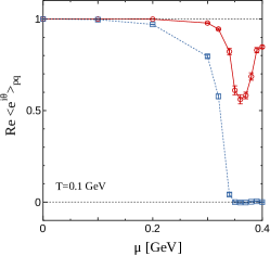
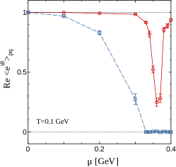
Figure 1: The $\mu$-dependence of $\mathrm{Re}\,\langle e^{i\theta}\rangle_{\mathrm{pq}}$ at $T=0.1$ GeV. The top and bottom panels show results with $k=8$ and $64$, respectively. The circle and square symbols are results after and before the optimization, respectively.

In some regions of $\mu$, the average phase factor becomes almost $0$ before the optimization as shown by the dashed line in the figure. By comparison, we can successfully increase the average phase factor after the optimization. It suggests that there are no need to complexify $\sigma$ and ${\vec{\pi}}$ auxiliary fields in the path optimization method to investigate the PNJL model with the repulsive vector-type interaction. Also, this would be true in the Lefschetz-thimble method and other complexified integral-path approaches. Compared with the PNJL model without the repulsive vector-type interaction Kashiwa et al. (2019), the average phase factor becomes worse because $\omega_{4}$ field additionally induces the sign problem at finite density. Around $\mu=0.36$ GeV, the optimization is neither sufficient nor automatic in the case with $k=64$. With naive initial conditions of dynamical variables, the average phase factor stays to be very small. Then, various initial conditions have been examined and we finally obtain the optimized path with reasonably large average phase factor as shown in Fig. 1. This result indicates that the present neural network in the case with $k=64$ does not have enough performance of the approximation to overcome the exponential suppression of the average phase factor.

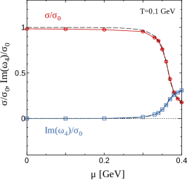
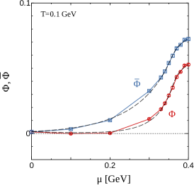
Figure 2: The top and bottom panels show the $\mu$-dependence of $\sigma$ and $\omega_{4}$, and $\Phi$ and ${\bar{\Phi}}$ at $T=0.1$ GeV with $k=64$ were $\sigma$ and $\omega_{4}$ are normalized by $\sigma$ at $T=\mu=0$ ($\sigma_{0}<0$) in the infinite volume limit. The thin dashed lines are the eye guide which are the mean-field results with the ${\cal CK}$ symmetry ansatz in the fermion determinant and the un-Wick rotated calculation.

Figure 2 shows the $\mu$-dependence of the order parameters at $T=0.1$ GeV after the optimization. We also show the mean-field results based on the ${\cal CK}$ symmetry ansatz in the fermion determinant Nishimura et al. (2014, 2015) where ${\cal C}$ and ${\cal K}$ are the charge and complex conjugations, respectively. This ansatz can be justified by using the Lefschetz thimble method Tanizaki et al. (2015). Under the ${\cal CK}$ symmetry condition, we solve gap equations

$$\frac{\partial\Gamma}{\partial\sigma}=0,~{}~{}~{}~{}\frac{\partial\Gamma}{\partial\omega_{0}}=0,~{}~{}~{}~{}\frac{\partial\Gamma}{\partial\Phi}=0,~{}~{}~{}~{}\frac{\partial\Gamma}{\partial{\bar{\Phi}}}=0,~{}~{}~{}~{}$$ (18)

where we do not use the Wick rotation of the vector-type auxiliary field. This treatment cannot be justified in the standard path integral formulation, but practically it reproduces the correct result in the leading-order of the large $N_{c}$ expansion because $\omega_{0}$ corresponds to the quark number density in the mean-field approximation. From the figure, we find that the numerical errors are well controlled and the difference between $\Phi$ and ${\bar{\Phi}}$ at finite density, ${\bar{\Phi}}>\Phi$, is correctly reproduced. Compared with the results without the vector-type interaction Kashiwa et al. (2019), the chiral condensate decreases more slowly. This is reasonable, since the repulsive vector-type interaction is known to weaken the chiral phase transition. We find that $|\mathrm{Im}\,\omega_{4}|$ strongly increases above $\mu=0.3$ GeV. Since the quark number density and $\omega_{4}$ are related with each other via $\omega_{0}=\langle q^{\dagger}q\rangle=i\omega_{4}$, this sudden increase indicates the absence of the Silver-Blaze problem at $T=0$; the quark number density should start to increase at $\mu=M(\mu=0)$. By comparison, results at small $\mu$ are almost the same as those without the vector-type interaction Kashiwa et al. (2019), since the quark number density and thus the vector potential are small.

It should be noted that the real part of $\omega_{4}$ is consistent with zero within the error-bar and thus the consequence obtained in the analyses in the Lefschetz thimble method  Mori et al. (2018a) is naturally understood in the path optimization method. We must consider Wick rotation of $\omega_{0}$, then the model sign problem can be resolved by complexifying $\omega_{4}$. The present results imply that the $\omega_{4}$ field has almost only the imaginary part, then the flow equation of the Lefschetz thimble can stall at a small value of $|\mathrm{Re}\,\omega_{4}|$. In Fig. 3, we show the scatter plot of the hybrid Monte-Carlo configurations at $T=0.1$ GeV and $\mu=0.3$ GeV on the $\mathrm{Re}\,A_{3}$-$\mathrm{Re}\,A_{8}$, $\mathrm{Re}\,A_{3}$-$\mathrm{Re}\,\omega_{4}$ and $\mathrm{Re}\,A_{8}$-$\mathrm{Re}\,\omega_{4}$ planes. We can see the localized configurations around $\mathrm{Re}\,A_{8}=0$ and $\mathrm{Re}\,A_{3}\neq 0$.

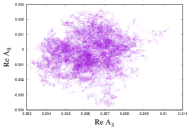
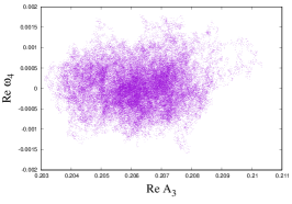
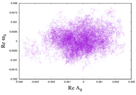
Figure 3: The scatter plot at $T=0.1$ GeV and $\mu=0.3$ GeV on the $\mathrm{Re}\,A_{3}$-$\mathrm{Re}\,A_{8}$, $\mathrm{Re}\,A_{3}$-$\mathrm{Re}\,\omega_{4}$ and $\mathrm{Re}\,A_{8}$-$\mathrm{Re}\,\omega_{4}$ planes. Here we use $80000$ configurations.

Thus, this study implies that the standard PNJL model computation with the repulsive vector-type interaction under the ${\cal CK}$ symmetry ansatz and the un-Wick rotated $\omega_{0}$ in the mean-field approximation is systematically and numerically justified via the path optimization method. The scatter plot also supports the direct complexification of $A_{3}$ and $A_{8}$ without taking care of the periodicity. The Monte-Carlo configurations are not spread but localized, then it is not necessary to take account of the periodic boundary condition.

IV Summary

In this study, we have applied the path optimization method to the QCD effective model with the Polyakov loop and the repulsive vector-type interaction. The feedforward neural-network with the mono-hidden layer is employed to describe the good integral path in the complexified space of integral variables. The temporal components of the gluon field and the vector-type auxiliary field are complexified and then the path is optimized via the path optimization method.

By optimizing the path (manifold), we can successfully improve the average phase factor, and calculated results of observables show reasonable behavior and have small error bars. It is not easy to optimize the integral path in the rapidly changing region of the order-parameters, but we can finally improve the average phase factor by examining various initial conditions of dynamical variables.

After a few optimization steps, we can well reproduce the mean-field results at large volume as we expect. Since we use the homogeneous ansatz of the integral valuables, our numerical simulation should give the mean-field result in the large volume limit. The imaginary part of the vector-type auxiliary field starts to rapidly increase in strength above $\mu=0.3$ GeV at $T=0.1$ GeV. This indicates the absence of the Silver-Blaze problem at $T=0$ and thus the path optimization method can pick up correct properties of the theory.

In the standard mean-field approximation, we do not perform the Wick rotation of the vector auxiliary field ($\omega_{0}$). While such a treatment cannot be justified within the standard path integral formulation, it can be justified by employing the complexified theory such as the Lefschetz thimble method and the path optimization method. In this article, we have demonstrated that the path optimization method correctly resolve the model sign problem and then the $\omega_{4}$ field takes almost the pure imaginary value which is required from the fact that the grand-canonical partition function is real. This study provides the correct numerical treatment of the repulsive vector-type interaction in the QCD effective model with the Polyakov loop.

Finally, we comment on the problem of the numerical cost. The degree of freedom is enlarged in the present calculation compared with the case without vector-type interaction Kashiwa et al. (2019), the improvement of the average phase factor becomes slow, and thus we need more optimization steps (epochs) and/or some other extensions. One of the possible extensions to circumvent such optimization problem is introducing the deep neural-network and it is our future work. Also, the sign problem becomes exponentially severe with increasing system size. Then, it is important to know that the improvement of the average phase factor via the path optimization method can overcome the exponential suppression. Therefore, we need further investigation of the competition in the average phase factor between the suppression from the system size and the improvement from the path optimization. In particular, this problem becomes serious when we consider the lattice calculation. One promising approach is the reduction of the Jacobian computation cost; the diagonal ansatz of the Jacobian  Alexandru et al. (2018) and the nearest-neighbor lattice-cites ansatz Bursa and Kroyter (2018) are promising examples. It will be reported elsewhere.