Control Strategy Design for Power Quality Management in Active Distribution Networks

Abstract

Uncertainty and variability of renewable energy sources present an imperative technical challenge for Electrical Distribution Utilities. Power Quality (PQ) indices represent quality of energy delivered and reliability. In this work, a control strategy design for real-time PQ management in active distribution systems is presented. The present work addresses management of voltage fluctuations induced by the variability in renewable generation. A “zero energy reserve” approach to tackle fluctuations of renewable energy generators is developed. The power consumption of flexible loads is modulated to reduce the technical losses and peak load of the feeder in this reactive power (VAR) control strategy. A Volt/VAR control strategy formulation, using the capability of smart inverters to provide dynamic reactive power is presented. Unbalanced power flow, different load profiles and flexible loads as “virtual energy storages” are used to improve voltage profile and reduce technical losses while maintaining system reliability. IEEE 13 bus distribution system is used for control strategy design validation. Comparative results indicate reduction in the system technical losses and the stress on automatic voltage regulators (AVR). The ease of design of control strategy indicate potential real-life application.

I Introduction

Voltage regulation (VR) in distribution systems is traditionally performed at distribution network substation level. Capacitor banks adapt to the reactive power requirement of the system on a slower timescale (typically every hour). Due to uncertainty of available power from renewable energy sources and the upward trend of solar plant penetration into the distribution grid, there is a need for VAR control on a faster time scale [1]. Smart inverters, interfacing the solar plants at the point of interconnection are excellent controllable resources, which can follow a remote command to change their power factor. Three-phase inverters are ultimate reactive power generators, with response times of $1$ ms to full output [2]. Flexible loads in this document are defined as loads that can follow a regulation signal, providing ancillary services to the network. In [3], the authors show that HVAC systems in commercial buildings can provide demand side system frequency regulation.

Comprehensive studies have been made on Volt/VAR control for distribution systems. Most works consider the problems of optimal sizing, placement and switching schedules of capacitor banks and on-load tap changers (OLTC) [4], [5] and [6]. Inverter control on a fast timescale has been studied in some recent works [7], [8] and [9]. In [7], authors present a Volt/VAR control problem that minimizes both technical losses and power consumption. The core idea of this strategy was minimization of the weighted sum of voltages along the feeder using a balanced power flow model. In distribution systems, the unbalanced power flow is a model closer to reality than the DistFlow equations introduced in [4] and used in [7]. The potential benefits of flexible loads and real time power quality management were also not addressed in [7].

In this work, a centralized control strategy for real-time PQ management on distribution networks is presented. The present control strategy optimizes the technical losses, deviation from nominal voltage and power consumption of flexible load in a cost-effective approach considering the inherent distribution network characteristics. The inherent unbalanced operation, different load types, Markov chain modelling for solar generation and load forecasting, modulation of power consumption of flexible loads and the issues of following the fluctuations of renewable energy generation are considered in this work. The traditional VAR control using capacitor banks on a slow timescale has been studied in previous works. In this work, the control of smart inverters on a short timescale for real-time PQ management is investigated.

The remainder of the paper is organized as follows. In Section II, we present the problem formulation. In Section III, the fundamental aspects of Markov chain modelling of solar energy and load forecasting are addressed. In Section IV, a zero energy reserve approach is proposed and the control of an Energy Storage System (ESS) to follow the output fluctuations of renewable energy generators is discussed. In Section V, the proposed power quality control strategy design is reported. Comparative simulation results, discussion and analysis are presented in Section VI. Finally, some conclusions are given in Section VII.

II Problem Formulation

II-A Control Problem Statement

Volt/VAR regulation is a control problem on two timescales. Slow timescale control is done hourly (every $t$) and inverter fast timescale control is done every minute (every $t^{\prime}$). Current SCADA limits the timescale of control strategy to a minute. In this work, the inverter power factor which can be changed dynamically to match the uncertainty of renewable energy generators will be used for fast timescale Volt/VAR control. The configuration of capacitor banks is changed in the slow timescale control. This will reduce the number of tap changes of OLTC, thereby increasing their lifecycle.

II-B Distribution Grid Model

Consider a distribution network with $n$ buses, where $\mathcal{B}$ is a set of all the buses on the system $\mathcal{B}=(1,2,\ldots,n_{B})$. Let $\Phi=\{a,b,c\}$ the set of phases. Consider the distribution network that utilizes capacitor banks and tap changing transformers for voltage regulation. The state of the capacitor banks and tap changing transformers at time $t$ is modeled by an integer vector $s(t)\in\mathcal{A}$, where $\mathcal{A}$ is the set of feasible values of vector $s(t)$. The admittance matrix of the grid at time $t$ is given by $Y(s(t))$. The elements of the admittance matrix $Y_{ij-km}=G_{ij-km}+jB_{ij-km}$ are

$$Y_{ij-kk} =bsh_{i-k}+\sum_{m\in\Omega_{k}}\left(y_{ij-km}+bsh_{ij-km}\right)$$ (1)

$$Y_{ij-km} =-y_{ij-km}$$ (2)

where $\Omega_{k}$ is the set of buses adjacent to bus $k$, $y_{ij-km}$, $bsh_{ij-km}$ are series admittance and susceptance, respectively, of lines connected between buses $(i,j)\in\mathcal{B}$ and phases $(k,m)\in\Phi$, and $bsh_{i-k}$ is the shunt capacitance at bus $i$, phase $k$ which when there is presence of capacitor bank, is determined by state $s(t)$ of the capacitor banks.

II-C Generator Model

The complex power injected by the aggregated generators at node $k$ and time $t$ is denoted as $S_{k}^{G}(t)=P_{k}^{G}(t)+jQ_{k}^{G}(t)$. The active and reactive power that each generator can provide is bounded by

$$P_{k}^{G,\min}(t)\leq P_{k}^{G}(t)\leq P_{k}^{G,\max}(t)$$ (3)

$$Q_{k}^{G,\min}(t)\leq Q_{k}^{G}(t)\leq Q_{k}^{G,\max}(t)$$ (4)

If there is no generator at bus $k$, then $P_{k}^{G}(t)=Q_{k}^{G}(t)=0$. Time dependence of the active power takes into account generation from renewable sources that is time-varying. If the generator at bus $k$ uses only renewable energy sources, it is assumed in this work that the generation profile $P_{k}^{G}(t)$ is known/estimated in advance for the interval of time under study. Also, since one cannot schedule renewable resources, $P_{k}^{G,\min}(t)=P_{k}^{G,\max}(t)$ is assumed.

II-D Unbalanced Power Flow Formulation

Let $P^{\exp}$ and $Q^{\exp}$ denote the expected/estimated net injected real and reactive power while $P$ and $Q$ denote the realized injected real and reactive power. The difference between the estimated and the realized real and reactive powers is given by the following equation:

$$\begin{bmatrix}\Delta P\\ \Delta Q\end{bmatrix} =\begin{bmatrix}P^{\mathrm{exp}}\\ Q^{\mathrm{exp}}\end{bmatrix}-\begin{bmatrix}P\\ Q\end{bmatrix}$$ (5)

The goal is to estimate system states (bus voltage magnitudes and angles) which minimizes functions $\Delta P$ and $\Delta Q$ to a pre-established convergence tolerance. Realized power in (5) can be given by the following expressions:

$$P_{i-k} =V_{i-k}\sum_{j\in\mathcal{B}}\sum_{m\in\Phi}V_{j-m}(G_{ij-km}\cos\theta_{ij-km}+$$

$$\quad B_{ij-km}\sin\theta_{ij-km})$$ (6)

$$Q_{i-k} =V_{i-k}\sum_{j\in\mathcal{B}}\sum_{m\in\Phi}V_{j-m}(G_{ij-km}\sin\theta_{ij-km}-$$

$$\quad B_{ij-km}\cos\theta_{ij-km})$$ (7)

where $P_{i-k}$ and $Q_{i-k}$ represent the active and reactive power injections at bus $i$, phase $k$. $V_{i-k}$ and $V_{j-m}$ represent the magnitude of voltage phasor at bus $i$, phase $k$ and bus $j$, phase $m$, respectively. $G_{ij-km}$ is the conductance of the lines connected between bus $i-j$ and phase $k-m$, respectively. $B_{ij-km}$ is given as in (1) and (2). $\theta_{ij-km}$ is the angular difference between bus $i$, phase $k$ and bus $j$, phase $m$.

The system of non-linear algebraic equations modelling the power flow in the distribution grid is solved using Newton-Raphson (NR) approach. The initial system state is normally considered as a flat voltage profile. NR approach solves (5) iteratively, by linearizing the system at each time step. The linearized system of equations is given by

$$J\begin{bmatrix}\Delta\theta\\ \Delta V\end{bmatrix} =\begin{bmatrix}\Delta\theta\\ \Delta V\end{bmatrix}$$ (8)

with the states being updated according to the following equation,

$$\begin{bmatrix}\theta\\ V\end{bmatrix}^{\nu+1} =\begin{bmatrix}\theta\\ V\end{bmatrix}^{\nu}+\begin{bmatrix}\Delta\theta\\ \Delta V\end{bmatrix}^{\nu}$$ (9)

The process is repeated until functions $\Delta P$ and $\Delta Q$ are smaller than a pre-established convergence tolerance.

The Jacobian matrix can be derived by considering different types of loads. Consider the load model given by the following equations

$$P_{k-i}^{\mathrm{exp}} =P_{k-i}^{\mathrm{nom}}\sum_{l=1}^{n}a_{l}\left(\frac{V_{k-i}}{V_{k-i}^{\mathrm{nom}}}\right)^{{n_{p}}_{l}}$$ (10)

$$Q_{k-i}^{\mathrm{exp}} =Q_{k-i}^{\mathrm{nom}}\sum_{l=1}^{n}b_{l}\left(\frac{V_{k-i}}{V_{k-i}^{\mathrm{nom}}}\right)^{{n_{q}}_{l}}$$ (11)

where $P_{k-i}^{\mathrm{exp}}$ and $Q_{k-i}^{\mathrm{exp}}$ are expected real and reactive power of bus $k$ for a given voltage $V_{k}$, $V_{k}^{\mathrm{nom}}$ is the bus $k$ nominal voltage, $a_{l}$ and $b_{l}$ are the bus $k$ expected percentages of $\left(P_{k-i}^{\mathrm{exp}},Q_{k-i}^{\mathrm{exp}}\right)$ with respect to coeficients $n_{p_{l}}$ and $n_{q_{l}}$, with $\sum_{l=1}^{\ell}a_{l}=1$, $\sum_{l=1}^{\ell}b_{l}=1$, where $\ell$ denotes the different load types present of the bus.

The Jacobian matrix is:

$$J =\left[\begin{array}[]{cc}\displaystyle\frac{\partial P}{\partial\theta}&\displaystyle\frac{\partial P}{\partial V}\\[8.61108pt] \displaystyle\frac{\partial Q}{\partial\theta}&\displaystyle\frac{\partial Q}{\partial V}\end{array}\right]$$ (14)

and its elements are:

$$\frac{\partial P_{i-k}}{\partial\theta_{i-k}} =-V_{i-k}^{2}B_{ii-kk}-Q_{i-k}$$ (15)

$$\frac{\partial P_{i-k}}{\partial\theta_{j-m}} =V_{i-k}V_{j-m}(G_{ij-km}\sin\theta_{ij-km}-$$

$$\quad B_{ij-km}\cos\theta_{ij-km})$$ (16)

$$\frac{\partial P_{i-k}}{\partial V_{j-m}} =V_{i-k}(G_{ij-km}\cos\theta_{ij-km}+$$

$$\quad B_{ij-km}\sin\theta_{ij-km})$$ (17)

$$\frac{\partial Q_{i-k}}{\partial\theta_{i-k}} =-V_{i-k}^{2}G_{ii-kk}+P_{i-k}$$ (18)

$$\frac{\partial Q_{i-k}}{\partial\theta_{j-m}} =-V_{i-k}V_{j-m}(G_{ij-km}\cos\theta_{ij-km}+$$

$$\quad B_{ij-km}\sin\theta_{ij-km})$$ (19)

$$\frac{\partial Q_{i-k}}{\partial V_{j-m}} =V_{i-k}(G_{ij-km}\sin\theta_{ij-km}-$$

$$\quad B_{ij-km}\cos\theta_{ij-km})$$ (20)

$$\frac{\partial P_{i-k}}{\partial V_{i-k}} =V_{i-k}G_{ii-kk}+\frac{P_{i-k}}{V_{i-k}}-$$

$$\quad P_{k-i}^{\mathrm{nom}}\sum_{l=1}^{n}{n_{p}}_{l}a_{l}\left(\frac{V_{k-i}}{V_{k-i}^{\mathrm{nom}}}\right)^{{n_{p}}_{l}-1}$$ (21)

$$\frac{\partial Q_{i-k}}{\partial V_{i-k}} =-V_{i-k}B_{ii-kk}+\frac{Q_{i-k}}{V_{i-k}}-$$

$$\quad Q_{k-i}^{\mathrm{nom}}\sum_{l=1}^{n}{n_{q}}_{l}b_{l}\left(\frac{V_{k-i}}{V_{k-i}^{\mathrm{nom}}}\right)^{{n_{q}}_{l}-1}$$ (22)

III Solar Forecasting and Load Modeling: A Markov Chain Approach

III-A Introduction

A Markov chain is a probabilistic model that represents system dynamics with a finite number of states [10], [11]. A Markov chain is characterized by a pair of elements $(\mathcal{N},\Pi)$ where $\mathcal{N}=\{1,2,\ldots,N\}$ is the set of finite states and $\Pi$ is the matrix of transition probabilities. Let $X_{t}$ be the state of the Markov chain at time $t$. The state can change according to the corresponding transition probability $\pi_{ij}=\mathrm{Pr}\{X_{t+1}=j|X_{t}=i\}$. Thus, the matrix $\Pi$ has nonnegative entries and the sum of each row is equal to one.

III-B Solar Insolation

III-B1 Markov chain modelling

Markov chains have been previously used to model and simulate solar insolation [12], [13]. In our Markov chain model, using recorded measurements of solar insolation from NREL National Radiation Data Base [14], the maximum and minimum solar insolation profile for each hour of each month of the year can be estimated. The variation range is split in $N$ levels that are labeled by the elements of the state set $\mathcal{N}$. The upper level of radiation is labeled by $1$ and the lower level by $N$ and the transitions probabilities can be estimated from the data. Therefore, the transition probabilities encode the system dynamic characteristics. In this work, a total of twelve Markov chain models, one for each month of the year, are used.

III-B2 Solar insolation simulation

A simulation of the solar insolation for a given day is realized as follows. Select the Markov chain model for the corresponding month of the year and the variation range for each hour. Select the initial state and run a simulation for each hour of the day. At each time instant $t$ a random uniform noise is added such that the solar insolation is random but remains in the corresponding level given by the Markov chain state.

III-B3 Solar insolation forecasting

The Markov chain model can be applied to forecast the solar insolation. A Markov chain corresponding to the month of the day that one wants to forecast and the variation range for the corresponding hour is considered. The forecasted solar insolation $\hat{P}_{t+k}^{S}$ at time $t+k$ assuming that the state at time $t$ is $X^{S}_{t}=i$ can be obtained using the conditioned expected value of the future state $\mathbb{E}[X^{S}_{t+k}|X^{S}_{t}=i]$ and the range of variation $R^{S}(t+k)$ for the hour of the day corresponding to time instant $t+k$, i.e.

$$\hat{P}^{S}_{t+k} =\frac{1}{N}R^{S}(t+k)\left(\mathbb{E}[X^{S}_{t+k}|X^{S}_{t}=i]-\frac{1}{2}\right)$$

$$=\frac{1}{N}R^{S}(t+k)\left(\sum_{j=1}^{N}b_{j}^{\top}\Pi_{S}^{k}b_{i}-\frac{1}{2}\right)$$

where $b_{i}$ is the $i$-th column vector of the identity matrix $I_{N_{S}}$ of dimension $N_{S}$, and $\Pi_{S}^{k}=\Pi_{S}^{1}\cdot\Pi_{S}^{k-1}$ and $\Pi_{S}^{0}=I_{N_{S}}$.

III-C Load Forecasting

III-C1 Load Modelling

The modeling, simulation and forecast of load variation can be done similarly using a discrete Markov chain. Using data from the past, one can obtain the maximum and minimum load for a certain time interval (typically one hour) of a given week day, for example a Tuesday of June. These maximum and minimum values define the variation range of the load for this hour. This range is split in $N$ levels and a state of the Markov chain is assigned to each level. The state corresponding to the upper subinterval of load variation is labeled by $1$ and the lower one by $N$. The transition probabilities are estimated from the data.

III-C2 Simulating the loads

A simulation of the load variation for a given day is realized as follows. Select the Markov chain model and the variation range for each time interval of the corresponding week day and month of the year. Select an initial state and run a simulation for each hour of that day. At each time instant the load is given by the realization of a random variable whose expectation is the mean value of the subinterval corresponding to the Markov chain state and with range or variation given by the range of the subinterval

III-C3 Flexible Load Forecasting

The Markov chain model can also be used to forecast the flexible load variation. For instance, the Markov chain corresponding to the week day and the month that one wants to forecast and the variation range for the corresponding time can be selected for the corresponding time interval. The forecasted load $\hat{P}^{L}_{t+k}$ at time $t+k$ assuming that the state at time $t$ is $X_{t}^{L}=i$ is obtained using the conditioned expected value of the future state $\mathbb{E}[X^{L}_{t+k}|X^{L}_{t}=i]$ and the range of variation $R^{L}(t+k)$ for the hour of the day corresponding to time instant $t+k$, i.e.

$$\hat{P}^{L}_{t+k} =\frac{1}{N}R(t+k)\left(\mathbb{E}[X_{t+k}^{L}|X_{t}^{L}=i]-\frac{1}{2}\right)$$

$$=\frac{1}{N}R^{L}(t+k)\left(\sum_{j=1}^{N}b_{j}^{\top}\Pi_{L}^{k}b_{i}-\frac{1}{2}\right)$$

where $b_{i}$ is the $i$-th column vector of the identity matrix $I_{N_{L}}$ of dimension $N_{L}$, and $\Pi_{L}^{k}=\Pi_{L}^{1}\cdot\Pi_{L}^{k-1}$ and $\Pi_{L}^{0}=I_{N_{L}}$.

The load profiles of a $13.8$ KV feeder in Florida, which were used in the simulations are illustrated in Fig. 1 and Fig. 2. Different load profiles were used to simulate different seasons (Fig. 3). The profiles of different loads were derived from the feeder load profiles using their generic models (obtained by using averaged load profile for different types of loads).

At any given state of the load, the amount of load which can be modulated is determined by the minimum and maximum envelopes of load consumption [3] as shown in the Fig. 2, where $P_{\min}^{L}=\min R^{L}(t)$, $P_{\max}^{L}=\max R^{L}(t)$, and $R^{L}(t)$ is the variation range of the load at time $t$.

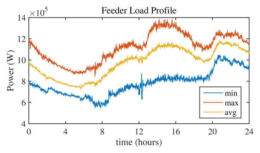
Figure 1: Feeder Load Profile (Summer)

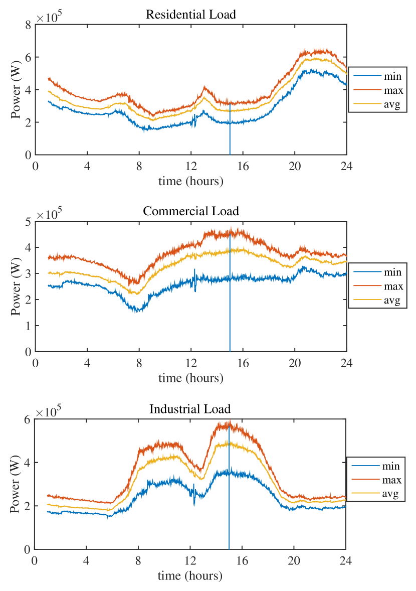
Figure 2: Different Load Profiles (Summer)

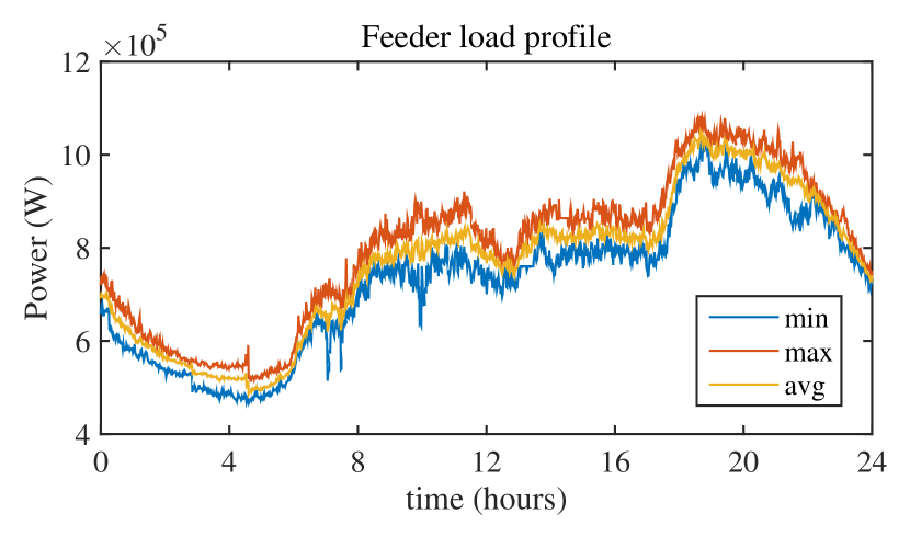
Figure 3: Feeder Load Profile (Winter)

IV Zero Energy Reserve Approach

In this work, the energy storage system (ESS), generators and flexible loads are used to match the renewable output fluctuations. The measurement of solar energy $S_{\mathrm{measured}}(t)$ and available solar energy $S_{\mathrm{forecast}}(t+1)$ are formulated as presented in Section III.

At any time, a “difference signal” $d(t)$ is derived from the $S_{\mathrm{measured}}(t)$ and $S_{\mathrm{forecast}}(t+1)$, which should be followed by ESS, generators and flexible loads,

$$d(t)=S_{\mathrm{forecast}}(t+1)-S_{\mathrm{measured}}(t)$$ (23)

A spectral decomposition of the difference signal into low and high frequency components for the control problem on two different timescales is proposed (not to be confused with $t$ and $t^{\prime}$). The idea of spectral decomposition is similar to the one presented for demand-side flexibility in [15]. The difference signal is analogous to the grid regulation signal used to balance generation and load [16]. The high frequency difference signal typically has a characteristic time of about one minute, while the low frequency difference signal has a characteristic time of about five minutes. In this work, a moving average sigmoid filter (20 samples) was used to formulate the low frequency difference signal $d_{l}(t)$,

$$d_{l}(t)=\sum_{k=1}^{20}w_{k}d(t-k)$$ (24)

where the finite impulse response was selected as a decreasing sigmoid function $w_{k}=1-(1+e^{-12k-0.5})^{-1}$ for $k\in\{1,2,\ldots,20\}$.

One can obtain a high frequency difference signal $d_{h}(t)$from the difference signal and the low frequency difference signal, which can be used to follow the minute variations in the solar output,

$$d_{h}(t)=d(t)-d_{l}(t)$$ (25)

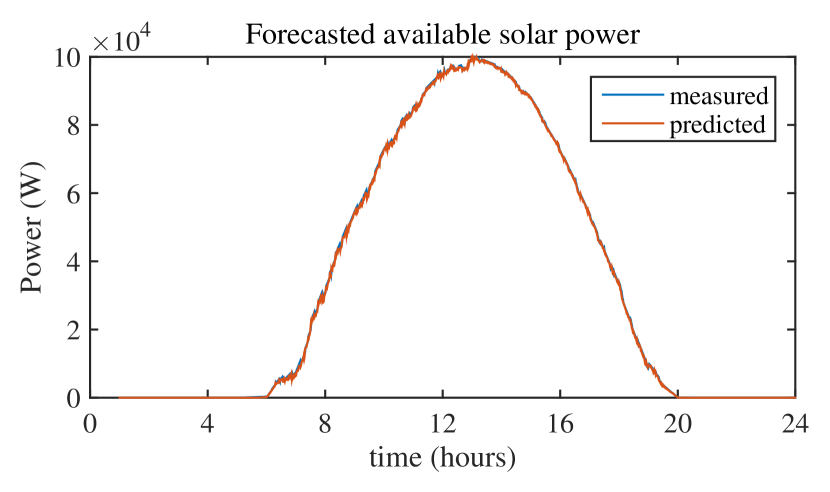
Figure 4: Forecasted and Measured Solar Power

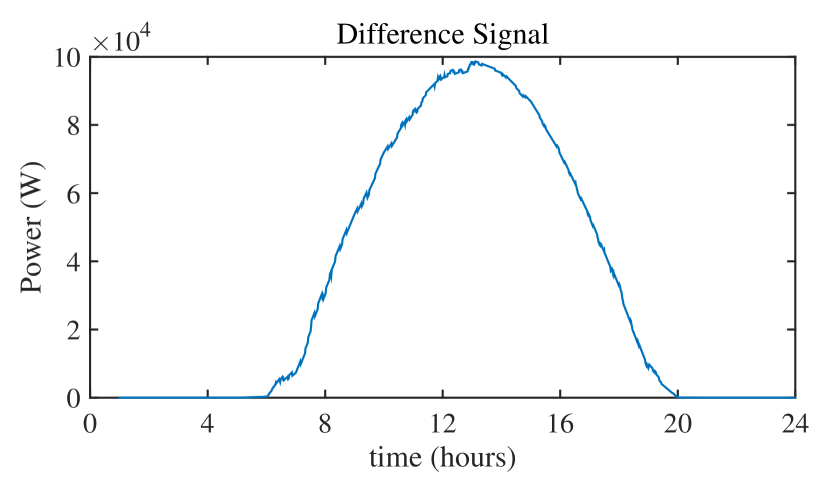
Figure 5: Difference Signal

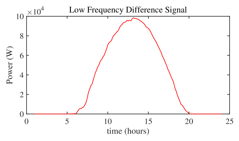
Figure 6: Low Frequency Difference Signal

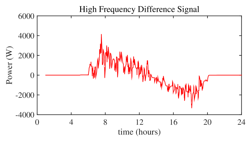
Figure 7: High Frequency Difference Signal

In Fig. 4 to Fig. 7 we show the forecasted and measured solar power, the difference signal, and the low and high frequency difference signals.

IV-1 Discussion

The averaged low frequency difference signal with a characteristic time of about five minutes can be followed by dispatch of generators (five-minute market) and/or modulation of power consumption of flexible load. The high frequency difference signal can be followed by ESS, which employ a “zero energy reserves” approach. The energy capacity of ESS installed can be reduced using this control strategy because they are only used to follow ramp ups and/or ramp downs unlike traditional control in which ESS follows the difference signal. A signal of frequency $r(t)/(A\pi)$ cycles/hour can be successfully tracked by the batteries with a capacity of $A$ MWh to smooth out the intermittencies in power caused by solar (here $r(t)$ is the maximum deviation from base-line). The energy capacity calculations for the data used in simulations are presented in the appendixA.

V Optimization Problem

Consider the Volt/VAR optimization problem on two timescales. As stated in [7], the slow timescale problem of capacitor bank switching is to find a state $s(t)$ of the discrete controllers (capacitor banks) which minimized a cost function, which represents the cost of switching from configuration $s(t-1)$ in previous time period to $s(t)$, the current time period. This slow timescale control is used to adapt to the aggregate reactive power requirement of the system. One can compute the optimal setting of discrete controller using various methods studied in the literature [17].

$s(t)$ determines the system configuration and it is constant over $t$ while the fast timescale control time $t^{\prime}$ changes. The fast timescale inverter control optimization problem is modeled by $C(s(t),t^{\prime})$, which is the sum of technical losses in each phase in the distribution system and the sum of weighted deviations of voltage in every phase from nominal voltage.

$$\min C(s(t),t^{\prime}) =\sum_{(i,j,k)\in B\times B\times\Phi}r_{ij,k}|I_{ij,k}|^{2}+$$

$$\qquad\sum_{(i,k)\in\mathcal{B}\times\Phi}\alpha_{ik}|v_{ik}(t^{\prime})-v_{\mathrm{nom}}|^{2}$$ (26)

subject to $$|P_{i}+jQ_{i}|\leq S_{i}$$ (27)

$$P_{\min}^{L}\leq P^{L}\leq P_{\max}^{L}$$ (28)

$$P_{i-k}^{\mathrm{exp}}-P_{i-k}=0$$ (29)

$$Q_{i-k}^{\mathrm{exp}}-Q_{i-k}=0$$ (30)

where $P_{\min}^{L}=\min R(t)$, $P_{\max}^{L}=\max R^{L}(t)$ and $R^{L}(t)$ is the variation range of the flexible load profile for instant $t$. The expressions for $P_{i-k}$ and $Q_{ik}$ were given in (6) and (7). Here, $\alpha_{ik}$ are the weights assigned for each bus and phase.

The term $r_{ij,k}|(I_{iji,k}|^{2}$ represents the technical losses in the line between buses $i$ and $j$ in phase $k$. In this work, ANSI C84-1, Range A (0.95 p.u to 1.05 p.u) is considered as the nominal voltage range. Recent studies [18] show that reduction of energy consumption can be achieved using Conservation Voltage Reduction (CVR). This can be achieved by reduction of feeder voltage. In this work, the optimization problem was solved by choosing $v_{i}{\mathrm{nom}}$ as $1$ p.u, because the goal is to achieve a flat voltage profile, thereby improving the $\mathrm{STARFI}_{x}$ PQ index [19]. The second term of optimization problem models the average power saving which can be achieved by CVR, which is quantified in terms of a profit function:

$$J(t) =K_{1}\Delta C+K_{2}\Delta P_{l}-K_{3}\mathrm{STARFI}_{x}$$ (31)

where $\Delta C$ and $\Delta P_{l}$ are lost capacity and reduction in technical losses of the line with 1547 control and fast inverter control, respectively. $K_{1}$, $K_{2}$ are constants with units $/KW, $K_{3}$ is the penalty for the utility (in $/number of customers) and $\mathrm{STARFI}_{x}$ is a long duration PQ index related to voltage deviation [19].

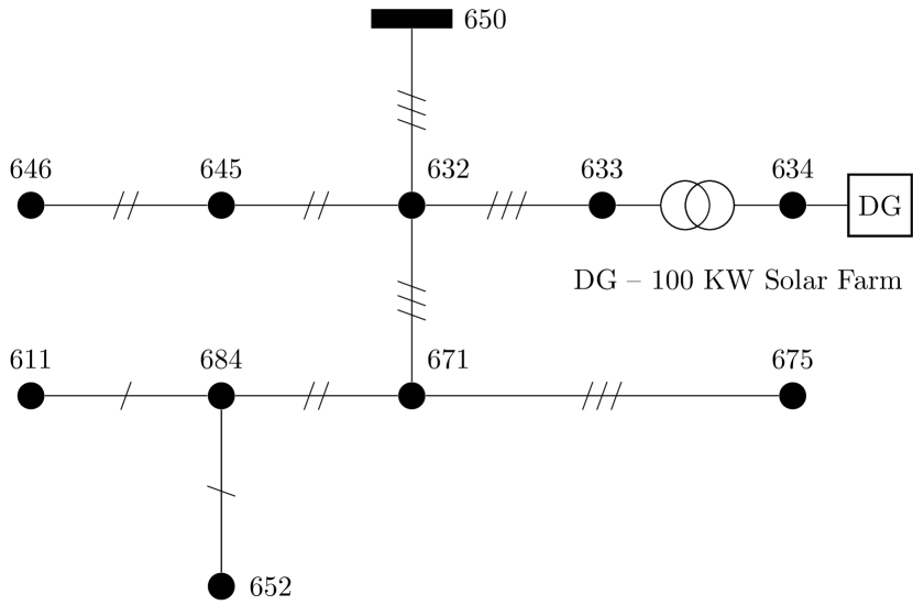
Figure 8: Simplified IEEE 13 Bus System

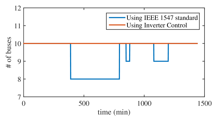
Figure 9: Number of buses in the acceptable operating voltage region for IEEE-1547 Standard and the Fast Inverter Control assuming a voltage tolerance of 5%.

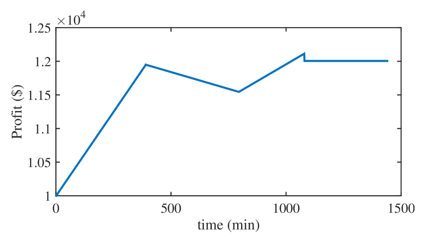
Figure 10: Average Utility Profit Function

VI Simulation Results

Consider the IEEE 13 bus test feeder system, illustrated in Fig. 8. The test feeder is modified to consider renewable energy penetration on bus 634. In this section, test results of fast inverter control when applied to a feeder with high renewable penetration to prove the robustness of the control algorithm are presented.

IEEE 1547 standard states that the “DG shall not actively regulate the voltage and shall not cause the system voltage to go outside the requirements of ANSI C84-1, Range A (0.95 p.u to 1.05 p.u)”. This forbids the distributed generators to regulate the voltage. The solar inverters operate at unity power factor w.r.t to the distribution system. We compare our results to this current PV integration standard.

A simplified IEEE 13 Bus system as shown in Fig. 8 was used. The bus 692 was eliminated by closing the switch and bus 680 was eliminated due to zero power injection from the standard IEEE 13 bus system. Also, a solar farm with $100$ KW of capacity was introduced at bus 634. The forecast of the available solar power and load forecasting was done as explained in Section III. The condition of high renewable penetration was simulated using the appropriate profiles of solar power available as shown in Fig. 4. The various load profiles for residential, industrial and commercial loads as shown in Fig. 2 were used. These loads were distributed along the feeder. HVAC system in commercial buildings were used as a flexible load. The slow timescale control was done by changing the capacitor bank configuration to follow the reactive power requirement of the aggregated feeder load profile.

In the following simulations, for every time step $t^{\prime}$, the solar farm was simulated as a PV bus to determine the maximum reactive power it can inject and then simulated as a PQ bus, after the optimal operating point has been determined by solving the optimization function as described in Section V.

TABLE I: SIMULATION RESULTS FOR TRANSFORMER TAP CHANGES

IEEE 1547 standard	Fast Inverter VAR Control
43	19

Test results demonstrate the robustness of the control strategy presented in this paper. All the buses serving the loads were in the acceptable range over a 24-hour period while there were some buses operating in unacceptable ranges for significant periods of time using IEEE1547 standard.

There is significant reduction in tap changes of OLTC. They are reduced by about half which increases the lifecycle and reduce operating costs. The utility profit function proposed in (16), an index for savings achieved by optimal reactive power dispatch of inverters, reducing the system losses and peak load in terms of cost (in $) was calculated for every time step $t’$. By assuming appropriate values for $K_{1}$, $K_{2}$ and penalty $K_{3}$, the averaged utility profit function is illustrated in Fig. 10.

VII Conclusions

Increasing intermittent renewable energy penetration presents imperative operation challenges to distribution utilities. In this work, a control strategy for real-time management of power quality design for distribution networks is presented. The approach considers the inherent characteristics of distribution networks such as unbalanced operation and different load types and ESS. The presented control strategy design addresses the induced voltage fluctuations due to variability in renewable generation. A “zero energy reserves” approach to tackle fluctuations of renewable energy generators is presented. The power consumption of flexible loads is modulated to reduce the technical losses and peak load of the feeder in a reactive power (VAR) control strategy. Unbalanced power flow, different load profiles and flexible loads as “virtual energy storage” are used to improve voltage profile and reduce system losses while maintaining system reliability. IEEE 13 bus distribution system is used for control strategy design validation. Comparative test results with IEEE 1547 standard indicate reduction in the system technical losses and the stress on automatic voltage regulators (AVR). The ease of design of control strategy indicate potential real-life application.

For the data used in the simulations:

Energy of slow difference signal $=789.15$ KWh.

Energy of the fast difference signal $=2.85\cdot 10^{-10}$ KWh. (zero energy reserve).

Energy Capacity of ESS to follow difference signal $=1.57$ KWh.

Energy capacity of ESS to follow fast difference signal $=63.65$ Whr. (to follow a maximum ramp $4.15$KW).

References

- [1] A. Moreno-Muñoz, Power quality: mitigation technologies in a distributed environment. Springer Science & Business Media, 2007.
- [2] C. Schauder, Advanced Inverter Technology for High Penetration Levels of PV Generation in Distribution Systems. National Renewable Energy Laboratory, 2014.
- [3] Y. Lin, P. Barooah, S. Meyn, and T. Middelkoop, “Demand side frequency regulation from commercial building hvac systems: An experimental study,” in American Control Conference (ACC), 2015.
- [4] M. E. Baran and F. F. Wu, “Optimal sizing of capacitors placed on a radial distribution system,” Power Delivery, IEEE Transactions on, vol. 4, no. 1, pp. 735–743, 1989.
- [5] M. Liu, C. Cañizares, W. Huang et al., “Reactive power and voltage control in distribution systems with limited switching operations,” Power Systems, IEEE Transactions on, vol. 24, no. 2, pp. 889–899, 2009.
- [6] Y. Liu, P. Zhang, and X. Qiu, “Optimal volt/var control in distribution systems,” International journal of electrical power & energy systems, vol. 24, no. 4, pp. 271–276, 2002.
- [7] M. Farivar, C. R. Clarke, S. H. Low, and K. M. Chandy, “Inverter var control for distribution systems with renewables,” in Smart Grid Communications (SmartGridComm), 2011 IEEE International Conference on. IEEE, 2011, pp. 457–462.
- [8] H.-G. Yeh, D. F. Gayme, and S. H. Low, “Adaptive var control for distribution circuits with photovoltaic generators,” Power Systems, IEEE Transactions on, vol. 27, no. 3, pp. 1656–1663, 2012.
- [9] M. Farivar, R. Neal, C. Clarke, and S. Low, “Optimal inverter var control in distribution systems with high pv penetration,” in Power and Energy Society General Meeting, 2012 IEEE. IEEE, 2012, pp. 1–7.
- [10] J. R. Norris, Markov Chains. Cambridge University Press, 1998.
- [11] P. Bremaud, Markov Chains. Gibbs Fields, Monte Carlo Simulation, and Queues. Springer, 1999.
- [12] J. S. Ehnberg and M. H. Bollen, “Simulation of global solar radiation based on cloud observations,” Solar Energy, vol. 78, no. 2, pp. 157–162, 2005.
- [13] J. Bright, C. Smith, P. Taylor, and R. Crook, “Stochastic generation of synthetic minutely irradiance time series derived from mean hourly weather observation data,” Solar Energy, vol. 115, pp. 229–242, 2015.
- [14] S. Wilcox and W. Marion, Users manual for TMY3 data sets. National Renewable Energy Laboratory Golden, CO, 2008.
- [15] P. Barooah, A. Buic, and S. Meyn, “Spectral decomposition of demand-side flexibility for reliable ancillary services in a smart grid,” in System Sciences (HICSS), 2015 48th Hawaii International Conference on. IEEE, 2015, pp. 2700–2709.
- [16] E. Ela, B. Kirby, E. Lannoye, M. Milligan, D. Flynn, B. Zavadil, and M. O’Malley, “Evolution of operating reserve determination in wind power integration studies,” in Power and Energy Society General Meeting, 2010 IEEE. IEEE, 2010, pp. 1–8.
- [17] S. Civanlar and J. Grainger, “Volt/var control on distribution systems with lateral branches using shunt capacitors and voltage regulators part iii: The numerical results,” Power Apparatus and Systems, IEEE Transactions on, no. 11, pp. 3291–3297, 1985.
- [18] K. P. Schneider, J. Fuller, F. Tuffner, and R. Singh, “Evaluation of conservation voltage reduction (cvr) on a national level,” Pacific Northwest National Laboratory report, 2010.
- [19] R. C. Dugan, M. F. McGranaghan, and H. W. Beaty, “Electrical power systems quality,” New York, NY: McGraw-Hill,— c1996, vol. 1, 1996.