Computational Analysis of Dispersive and Nonlinear 2D Materials by Using a Novel GS-FDTD Method

Abstract

In this paper, we propose a novel numerical method for modeling nanostructures containing dispersive and nonlinear two-dimensional (2D) materials, by incorporating a nonlinear generalized source (GS) into the finite-difference time-domain (FDTD) method. Starting from the expressions of nonlinear currents characterizing nonlinear processes in 2D materials, such as second- and third-harmonic generation, we prove that the nonlinear response of such nanostructures can be rigorously determined using two linear simulations. In the first simulation, one computes the linear response of the system upon its excitation by a pulsed incoming wave, whereas in the second one the system is excited by a nonlinear generalized source, which is determined by the linear near-field calculated in the first linear simulation. This new method is particularly suitable for the analysis of dispersive and nonlinear 2D materials, such as graphene and transition-metal dichalcogenides, chiefly because, unlike the case of most alternative approaches, it does not require the thickness of the 2D material. In order to investigate the accuracy of the proposed GS-FDTD method and illustrate its versatility, the linear and nonlinear response of graphene gratings have been calculated and compared to results obtained using alternative methods. Importantly, the proposed GS-FDTD can be extended to 3D bulk nonlinearities, rendering it a powerful tool for the design and analysis of more complicated nanodevices.

I Introduction

Since the first atomic-scale thin material (graphene) was successfully isolated from graphite in 2004 ngm04sci , a plethora of new two-dimensional (2D) materials have been discovered and synthesized mlh10prl ; scl10nl ; vpq12prl ; wkk12natnano ; g15nat ; blm15acsnano . Their novel and unique properties, combined with promising technological potential, have spurred a tremendous research interest geared towards both fundamental science and practical applications. For instance, graphene and transition-metal dichalcogenide (TMDC) monolayers wkk12natnano , which are just two examples of 2D materials, have already been employed in a broad array of applications, including electronics g09sci ; s10natnano ; ldj10sci ; rrb11natnano , sensors krz14natcom , energy storage lsc15nanoenergy , and solar cells zxy16nanoenergy .

In addition to their remarkable linear properties, the nonlinear optical properties of 2D materials could play an equally important role in the development of novel active photonic devices with new or improved functionality. For example, it has been demonstrated that third-order nonlinear optical interactions, such as third-harmonic generation (THG) hdp13prx ; cvs14njp ; csa16acsnano ; yyn17ptrsa and Kerr effect zvb12ol , are strongly enhanced in graphene when propagating or localized surface-plasmon polaritons (SPPs) are generated. Moreover, second-order nonlinear optical processes, such as second-harmonic generation (SHG) knc13prb ; mab13prb ; wmg15prl , are particularly strong in graphene placed on top of a substrate or TMDC monolayers because in these cases the 2D material system is not centrosymmetric. These nonlinear properties of 2D materials could find exciting applications both to advanced active photonic devices, such as nanoscale frequency mixers bsh10natphoton and photodetectors xml09natnano , and to the study of more fundamental phenomena, including spatial solitons nbn12lpr , tunable Dirac points dym15prb , and Anderson light localization at the nanoscale dcm15sr .

A key enabler of rapid developments in device applications of 2D materials is access to powerful computational methods that can describe the physics of such 2D systems, isolated or embedded in a 3D matrix. However, since one has to describe a mixture of 2D and 3D components that share the same physical space, one has to overcome serious challenges when traditional computational methods are to be extended to such heterostructures. Moreover, if one considers the optical properties of photonic structures containing 2D materials, both the linear and nonlinear induced polarizations depend strongly on frequency b08book , which means that the linear and nonlinear optical response of such structures are highly dispersive. These dispersive effects can be easily modeled in the frequency domain using several well-known numerical methods krg97jqe ; fk05jlt ; wp16prb ; nll16josab , as the dispersive, anisotropic and nonlinear polarization can be conveniently and efficiently calculated in the frequency domain. However, in order to fully describe the optical properties of the photonic system in the frequency domain, computations must be performed for all frequencies of interest, which can greatly increase the computational time.

To incorporate these dispersive and nonlinear effects in time-domain methods, such as the finite-difference time-domain (FDTD) method Taf05book , it would generally be required to calculate complex and computationally intensive time-domain convolution integrals JosTaf97tap ; GreTaf06OptExp ; GreTaf07MWCL ; Taf13book , which would consume significant computational resources. This drawback is particularly important as the computational time and memory requirements increase exponentially with the physical time over which the system dynamics is determined. To overcome this problem, several simplifications and algorithm improvements have been proposed JosTaf97tap ; GreTaf06OptExp ; GreTaf07MWCL ; Taf13book ; vc99mtt ; Sul95mtt to model instantaneous and dispersionless nonlinear phenomena. However, modeling optical properties of 2D materials faces additional challenges originating from embedding a 2D structure in a 3D computational grid. Whereas nonuniform grids can be implemented in the FDTD method, the large mismatch between the grids covering the domains containing 2D materials and bulk components and the enormous discrepancy between the optical wavelength and the thickness of 2D materials significantly reduces the efficiency of the FDTD method when it is applied to such 2D-3D heterostructures.

To overcome these challenges, in this paper we extend the well-known FDTD method to the case of optical structures containing optically nonlinear 2D materials by introducing the concept of nonlinear generalized source (GS). Specifically, we describe the nonlinear optical response of the 2D material via nonlinear surface currents lying on a 2D grid, and that are specific to the particular nonlinear optical process one wishes to study. These nonlinear currents are determined from a first linear FDTD simulation, using the specific expression relating them to the electric field at the fundamental frequency (FF). A second FDTD simulation, with these nonlinear currents as excitation sources, is then performed in order to compute the nonlinear optical response of the system. Since one only needs to know the specific functional dependence of the nonlinear currents on the field at the FF, this new numerical method, which we call GS-FDTD, can be applied to a broad array of nonlinear processes. The paper is organized as follows. In Section II, we describe the basic algorithm of the GS-FDTD. In addition, a general dispersive model for the electric permittivity of the 2D material considered in this work, i.e. graphene, is presented. In order to illustrate the versatility and efficiency of the proposed GS-FDTD method, we compute in Section III the linear and nonlinear response of generic graphene diffraction gratings and compare them with results obtained by using the rigorous coupled-wave analysis (RCWA) and finite-element time domain (FETD) method. Finally, the main results and conclusions of this study are summarized in Section IV.

II Computational Framework of GS-FDTD

In this section, we present the main ideas of our computational method. Thus, we first describe how we parameterize the frequency-dependent permittivity of 2D materials and the approach we used to translate these dependencies to the time domain. Then, we explain how nonlinear optical interactions are first described in the frequency domain via nonlinear surface currents and subsequently incorporated in the time domain formulation of our GS-FDTD method.

II.1 Incorporating 2D Nonlinear Materials in FDTD

We begin the description of our algorithm from the Maxwell equations. Thus, the Maxwell-Ampère law in the absence of free charges can be expressed as:

$$\nabla\times\textbf{{H}}={\textbf{{J}}_{d}}+{\textbf{{J}}_{c}}$$ (1)

where the displacement and conduction current densities, ${\textbf{{J}}_{d}}$ and ${\textbf{{J}}_{c}}$, respectively, are given by:

$${\textbf{{J}}_{d}}=\frac{\partial\textbf{{D}}}{\partial t},~{}~{}~{}~{}~{}~{}{\textbf{{J}}_{c}}=\sigma\textbf{{E}}.$$ (2)

with $\sigma$ being the electric conductivity.

In the frequency domain, we can decompose the electric flux density D into a linear part and a nonlinear part as follows:

$${\textbf{{D}}}(\omega)={\varepsilon_{0}}{\varepsilon_{r}}{{\textbf{{E}}}}(\omega)={{{\textbf{{D}}}}_{L}}(\omega)+{\textbf{{P}}_{NL}}({\Omega,\omega})$$ (3)

where ${\textbf{{P}}_{NL}}({\Omega,\omega})$ is the nonlinear polarization, which depends on the FF frequency, $\omega$, and the frequency of the higher-harmonic, $\Omega$, where $\Omega=2\omega$ ($\Omega=3\omega$) in the case of SHG (THG), and

$${{{\textbf{{D}}}}_{L}}(\omega)={\varepsilon_{0}}\left[{1+{\chi^{(1)}}(\omega)}\right]{{\textbf{{E}}}}(\omega)={\varepsilon_{0}}\varepsilon_{r}^{(1)}(\omega){{\textbf{{E}}}}(\omega)$$ (4)

In this equation, $\varepsilon_{r}^{(1)}(\omega)$ and $\chi^{(1)}(\omega)$ are the linear relative permittivity and susceptibility of the material, respectively. Using (3) and (4) in conjunction with (2), we arrive to the expression of the current density in the frequency domain:

$${\textbf{{J}}_{d}}(\omega)=\textbf{{J}}_{d}^{L}(\omega)+\textbf{{J}}_{d}^{NL}({\Omega,\omega})=-i\omega\left[{{{\textbf{{D}}}}_{L}}(\omega)+{\textbf{{P}}_{NL}}({\Omega,\omega})\right]$$ (5)

The generalized current density in this equation describes both the linear and nonlinear response of the material. Therefore, if one properly incorporates this quantity into the FDTD method, the complete response of the optical structure can be determined. For instance, the electromagnetic contribution of 2D materials are considered in our GS-FDTD method via generalized surface currents lying on 2D Yee’s grids, thus we can avoid constructing a bulk layer to approximate a 2D material in our simulations. However, for most 2D materials this generalized current density is frequency- and intensity-dependent. As such, if one incorporates this generalized current density directly into the regular FDTD method Taf05book , one needs to compute complex time-domain convolution integrals JosTaf97tap ; GreTaf06OptExp ; GreTaf07MWCL ; Taf13book . This would result in a prohibitive demand of computational time and memory resources. To overcome this roadblock, we incorporate the linear and the nonlinear parts of the generalized current density (5) into FDTD method in two separate steps. Specifically, we first determine the nonlinear current using a linear FDTD simulation, transform this nonlinear current in the time domain, then, in a second linear FDTD simulation, this current is used as a generalized source of the nonlinear field. These steps are described in detail in what follows.

II.2 Linear Simulation

In the linear FDTD simulation, we assume that there are only linear materials in the computational domain, and based on this assumption we calculate the corresponding time-dependent electromagnetic field distribution. In addition, the electric field at the location of (nonlinear) 2D materials, which can be viewed as the field at the FF, is recorded to be used in the next step of the algorithm, namely to evaluate the nonlinear GS currents.

The linear properties of most of 2D materials, including graphene and TMDC monolayers, are generally frequency-dependent. To include these dispersive effects in the FDTD method, one generally uses some well-known dispersion models, such as Debye, Drude, and Lorentz, to fit the frequency-dependent permittivity. As a result, the dispersive medium can be simulated by employing the auxiliary-difference-equation (ADE) FDTD method Taf05book . However, each dispersion model is only suitable for particular applications. For instance, the Debye model is generally used to describe the dispersive features of human tissues and soil, the Drude model is suitable for noble metals and plasma, and the Lorentz model is widely used to describe the optical dispersion of semiconductors and polaritonic materials.

Table 1: The coefficients $a_{m}^{0}$, $a_{m}^{1}$, $b_{m}^{0}$, $b_{m}^{1}$, $b_{m}^{2}$ describing several well-known dispersion models, namely Debye, Drude, Lorentz, and modified Lorentz.

Model	Dispersion	Coefficients
	${\varepsilon_{m}}\left(\omega\right)$	$\frac{{a_{m}^{0}+a_{m}^{1}\left({-i\omega}\right)}}{{b_{m}^{0}+b_{m}^{1}\left({-i\omega}\right)+b_{m}^{2}{{\left({-i\omega}\right)}^{2}}}}$
Debye	$\frac{{\Delta\varepsilon}}{{1-2i\omega{\gamma_{m}}}}$	$\begin{array}[]{l}\;\;\;\;\;\;a_{m}^{0}=\Delta\varepsilon,\;\;\;a_{m}^{1}=0,\\ b_{m}^{0}=1,\;\;\;b_{m}^{1}=2{\gamma_{m}},\;\;b_{m}^{2}=0\end{array}$
Drude	$\frac{{\Delta\varepsilon\cdot\omega_{m}^{2}}}{{-2i\omega{\gamma_{m}}-{\omega^{2}}}}$	$\begin{array}[]{l}\;\;a_{m}^{0}=\Delta\varepsilon\cdot\omega_{m}^{2},\;\;\;\;a_{m}^{1}=0,\\ b_{m}^{0}=0,\;\;\;b_{m}^{1}=2{\gamma_{m}},\;\;\;b_{m}^{2}=1\end{array}$
Lorentz	$\frac{{\Delta\varepsilon\cdot\omega_{m}^{2}}}{{\omega_{m}^{2}-2i\omega{\gamma_{m}}-{\omega^{2}}}}$	$\begin{array}[]{l}\;a_{m}^{0}=\Delta\varepsilon\cdot\omega_{m}^{2},\;a_{m}^{1}=0,\\ b_{m}^{0}=\omega_{m}^{2},\;b_{m}^{1}=2{\gamma_{m}},\;b_{m}^{2}=1\end{array}$
Lorentz-M	$\frac{{\Delta\varepsilon\cdot\omega_{m}^{2}-i\omega\Delta\varepsilon{\gamma^{\prime}_{m}}}}{{\omega_{m}^{2}-2i\omega{\gamma_{m}}-{\omega^{2}}}}$	$\begin{array}[]{l}\;a_{m}^{0}=\Delta\varepsilon\cdot\omega_{m}^{2},\;a_{m}^{1}=\Delta\varepsilon{\gamma^{\prime}_{m}},\\ b_{m}^{0}=\omega_{m}^{2},\;b_{m}^{1}=2{\gamma_{m}},\;b_{m}^{2}=1\end{array}$

The frequency dispersion of graphene permittivity cannot be described by any of these models. Therefore, we use a more general approach, which can be applied to practically any function describing the frequency dispersion of the optical medium. For the sake of specificity, we present here this approach applied to the particular case of graphene. Thus, the linear sheet conductance of graphene (sometimes simply called conductivity) is generally given by the Kubo’s formula. Within the random-phase approximation Hans08jap ; wzg15tnano , this formula can be reduced to the sum of inter-band and intra-band contributions. The intra-band part is given by:

$$\sigma_{intra}=\frac{{{e^{2}}{k_{B}}T\tau}}{{\pi{\hbar^{2}}\left({1-i\omega\tau}\right)}}\left[\frac{\mu_{c}}{k_{B}T}+2\ln\left(e^{-\frac{\mu_{c}}{k_{B}T}}+1\right)\right]$$ (6)

where $\mu_{c}$ is the chemical potential, $\tau$ is the relaxation time, $T$ is the temperature, $e$ is the electron charge, $k_{B}$ is the Boltzmann constant, and $\hbar$ is the reduced Planck’s constant. Moreover, if $\mu_{c}\gg k_{B}T$, which usually holds at room temperature, the inter-band part can be approximated as:

$$\sigma_{inter}=\frac{{i{e^{2}}}}{{4\pi\hbar}}\ln\left[{\frac{{2\left|{{\mu_{c}}}\right|-({\omega+i{\tau^{-1}}})\hbar}}{{2\left|{{\mu_{c}}}\right|+({\omega+i{\tau^{-1}}})\hbar}}}\right]$$ (7)

If we assume that the effective thickness of graphene is ${h_{eff}}$, its linear relative permittivity $\varepsilon_{r}^{(1)}(\omega)$ can be written as:

$$\varepsilon_{r}^{(1)}(\omega)=1+\frac{i\sigma_{s}}{\varepsilon_{0}\omega h_{eff}}$$ (8)

where $\sigma_{s}=\sigma_{intra}(\omega,\mu_{c},\tau,T)+{\sigma_{inter}}({\omega,\mu_{c},\tau,T})$.

It can be seen that the intra-band contribution to the permittivity, at THz and optical frequencies, is similar to that of noble metals, meaning that it can be described by a Drude model. On the other hand, the inter-band part is similar to the dispersion of a semiconductor, and therefore it can be represented by a Lorentz model. In order to correctly account for both contributions, we use a more general model for frequency dispersion, which is described in what follows.

Using a small set of dispersion coefficients, the dispersion models most used in practice, namely Debye, Drude, Lorentz, and modified Lorentz, can be described by a common formula:

$$\varepsilon_{r}^{(1)}(\omega)=\varepsilon_{\infty}+\sum\limits_{m=1}^{M}{{\varepsilon_{m}}(\omega)}$$ (9)

where $\varepsilon_{\infty}$ is the frequency-independent part of the permittivity, $M$ is the number of dispersion terms,

$${\varepsilon_{m}}(\omega)=\frac{{a_{m}^{0}+a_{m}^{1}(-i\omega)}}{{b_{m}^{0}+b_{m}^{1}(-i\omega)+b_{m}^{2}{{\left(-i\omega\right)}^{2}}}}$$ (10)

and $a_{m}^{0}$, $a_{m}^{1}$, $b_{m}^{0}$, $b_{m}^{1}$, and $b_{m}^{2}$ are dispersion coefficients defining the $m$th dispersion term. The particular values of these coefficients corresponding to the main dispersion models used in practice are given in Table 1.

Using this general dispersion model, the linear relative permittivity of graphene and other 2D materials can be accurately fitted. Thus, we have determined the dispersion coefficients for the particular case of graphene with ${\mu_{c}}=$0.6\text{\,}\mathrm{eV}$$, $\tau=$0.25\text{\,}\mathrm{ps}$$, and $T=$300\text{\,}\mathrm{K}$$, using five dispersion terms in (9) (one Drude term and four Lorentz terms), the corresponding values being presented in Table 2.

Table 2: Dispersion coefficients used to fit $\varepsilon_{r}^{(1)}(\omega)$ of graphene with ${\mu_{c}}=$0.6\text{\,}\mathrm{eV}$$, $\tau=$0.25\text{\,}\mathrm{ps}$$, and $T=$300\text{\,}\mathrm{K}$$.

$\varepsilon_{\infty}=1$	$a_{m}^{0}$	$a_{m}^{1}$	$b_{m}^{0}$	$b_{m}^{1}$	$b_{m}^{2}$
	($10^{30}$)	($10^{15}$[s])	($10^{30}$)	($10^{15}$[s])	(s2)
$m$=1	22.8	0	0	3.91	1
$m$=2	1.23	11.5	0.37	4.48	1
$m$=3	0.47	3.16$\times 10^{-5}$	0.13	9.39	1
$m$=4	7.56	6.44	3.78	0.74	1
$m$=5	2.05	5.59	1.02	2.4	1

The data presented in Figs. 1a and 1b show that there is a good agreement between the analytical formula and fitting results. Moreover, one can see that the linear permittivity of graphene at wavelengths larger than $2\text{\,}\mathrm{\SIUnitSymbolMicro m}$ steeply decreases (real part) or increases (imaginary part), which is a typical feature of permittivity of metals. On the other hand, graphene permittivity for $\lambda<$2\text{\,}\mathrm{\SIUnitSymbolMicro m}$$ is no longer monotonously dependent on wavelength, a common feature of semiconductors and polaritonic materials. Additionally, the results plotted in Figs. 1c and 1d suggest that the maximum relative error is within $10~{}\%$, if five dispersion terms are used. Here, the relative error is defined as $|\varepsilon_{r}^{(1)}(\omega)-\varepsilon_{fit}(\omega)|/|\varepsilon_{r}^{(1)}(\omega)|$, where $\varepsilon_{fit}(\omega)$ are the fitted values. Note that in order to achieve good fitting a relatively large number of dispersion terms must be included, which means that simply fitting the graphene dispersion with a Drude or Drude-Lorentz function can lead to large computational errors.

Based on (4), (5), and (9), the frequency-dependent form of the linear current density, $\textbf{{J}}_{d}^{L}(\omega)$ can be evaluated as:

$$\textbf{{J}}_{d}^{L}(\omega)= -i\omega{{{\textbf{{D}}}}_{L}}(\omega)=-i\omega{\varepsilon_{0}}\varepsilon_{r}^{(1)}(\omega){{\textbf{{E}}}}(\omega)$$

$$= -i\omega\varepsilon_{0}\left[\varepsilon_{\infty}+\sum\limits_{m=1}^{M}\varepsilon_{m}(\omega)\right]\textbf{{E}}(\omega)=\sum\limits_{m=0}^{M}\textbf{{J}}_{m}(\omega)$$ (11)

where $\textbf{{J}}_{0}(\omega)=-i\omega\varepsilon_{0}\varepsilon_{\infty}\textbf{{E}}(\omega)$ and

$${\textbf{{J}}_{m}}(\omega)={\varepsilon_{0}}\frac{{a_{m}^{0}(-i\omega)+a_{m}^{1}{{(-i\omega)}^{2}}}}{{b_{m}^{0}+b_{m}^{1}(-i\omega)+b_{m}^{2}{{(-i\omega)}^{2}}}}\textbf{{E}}(\omega),~{}~{}~{}m\geq 1.$$ (12)

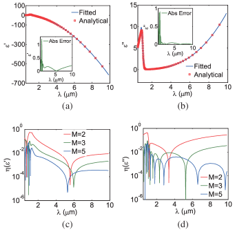
Figure 1: Relative permittivity of graphene (8) fitted with the general dispersion model (9), whose coefficients are listed in Table 2. (a), (b) Error analysis of real and imaginary parts of $\varepsilon_{r}^{(1)}(\omega)$, respectively. The insets show the absolute error. (c), (d) Convergence analysis of the relative error, where $M$ is the number of dispersion terms.

By using the ADE method Taf05book , the frequency-domain equation (12) can be cast into the following time-domain iterative relation:

$$\textbf{{J}}_{m}^{n+1}=c_{m}^{0}\textbf{{J}}_{m}^{n}+c_{m}^{1}\textbf{{J}}_{m}^{n-1}+c_{m}^{2}{\textbf{{E}}^{n+1}}+c_{m}^{3}{\textbf{{E}}^{n}}+c_{m}^{4}{\textbf{{E}}^{n-1}}$$ (13)

where the superscript $n$ indicates the $n$th time-step and the coefficients $c_{m}$’s for the $m$th dispersion term are given by:

$$c_{m}^{0} =\delta\left[2(\Delta t)^{2}b_{m}^{0}-4b_{m}^{2}\right],$$ (14a)

$$c_{m}^{1} =\delta(b_{m}^{1}\Delta t+2b_{m}^{2}),$$ (14b)

$$c_{m}^{2} =-\delta\varepsilon_{0}(a_{m}^{0}\Delta t-2a_{m}^{1}),$$ (14c)

$$c_{m}^{3} =-4\delta\varepsilon_{0}a_{m}^{1},$$ (14d)

$$c_{m}^{4} =\delta\varepsilon_{0}(a_{m}^{0}\Delta t+2a_{m}^{1}).$$ (14e)

where $\delta=1/(b_{m}^{1}\Delta t-2b_{m}^{2})$ and $\Delta t$ is the time-step used in the FDTD method. If one substitutes (13) and (14) into (1), one obtains the FDTD iteration for the linear simulation of dispersive 2D materials as:

$$\textbf{{E}}^{n+1}= {\beta_{1}}{\textbf{{E}}^{n}}+{\beta_{2}}\left[\nabla\times\textbf{{H}}^{n+\frac{1}{2}}\right.$$

$$- \left.\sum\limits_{m=1}^{M}\left(\beta_{3}^{m}\textbf{{J}}_{m}^{n}+\beta_{4}^{m}\textbf{{J}}_{m}^{n-1}\right)-{\beta_{5}}\textbf{{E}}^{n-1}\right]$$ (15)

where

$$\beta_{1} =\frac{\alpha_{1}-\alpha_{2}\sum\limits_{m=1}^{M}c_{m}^{3}}{1+\alpha_{2}\sum\limits_{m=1}^{M}c_{m}^{2}},\;\;\;\beta_{2}=\frac{\alpha_{2}\sum\limits_{m=1}^{M}c_{m}^{3}}{1+\alpha_{2}\sum\limits_{m=1}^{M}c_{m}^{2}},$$

$$\beta_{3}^{m} =\frac{c_{m}^{0}+1}{2},\;\;\beta_{4}^{m}=\frac{c_{m}^{1}}{2},\;\;\beta_{5}^{m}=\frac{1}{2}\sum\limits_{m=1}^{M}c_{m}^{4},$$

$$\alpha_{1} =\frac{2\varepsilon_{0}\varepsilon_{\infty}-\sigma\Delta t}{2\varepsilon_{0}\varepsilon_{\infty}+\sigma\Delta t},\;\;\;{\alpha_{2}}=\frac{\Delta t}{2\varepsilon_{0}\varepsilon_{\infty}+\sigma\Delta t}.$$

In these definitions, $\sigma$ is the bulk conductivity of bulk components of the photonic structure.

The basic steps for the linear simulation of 2D materials can be briefly summarized as follows: Step 1, update (II.2) to compute the field ${E^{n+1}}$ at the new time-step; Step 2, calculate $J_{m}^{n+1}$ in (13) by using ${E^{n+1}}$ obtained at Step 1; Step 3, let $n=n+1$ then repeat Step 1 and Step 2 until the energy in the entire computational region converges ytc14mtt .

II.3 Nonlinear Simulation

Similar to the case of bulk optical media, the nonlinear optical properties of 2D materials are generally determined by the symmetry properties of their atomic lattice and quantified via nonlinear susceptibility tensors. In particular, graphene lattice belongs to the $\mathcal{D}_{6h}$ point symmetry group, so that SHG is forbidden in a uniform graphene sheet. However, if graphene is placed on top of a substrate, the centrosymmetric property is not preserved because the up-down mirror symmetry is broken at the interface containing graphene, the point symmetry group in this case being $\mathcal{C}_{6v}$. As a result, considerable SHG can be observed in this case dh09apl ; m11prb ; ard14prb ; dh10prb ; chc16NatPhy . Moreover, strong THG in graphene can also occur hdp13prx ; cvs14njp ; csa16acsnano , as its third-order susceptibility is particularly large. Importantly, our method can be applied to other 2D materials, too, as it only requires the knowledge of the nonlinear optical conductivity describing the particular nonlinear process.

The nonlinear properties of graphene are quantified by a nonlinear surface conductivity tensor, $\bm{\sigma}_{s}^{(n)}(\Omega;\omega)$, where $n$ indicates the order of the nonlinear optical interaction. In the case of SHG, the second-order surface conductivity tensor only has three independent nonzero components, $\sigma_{s,\perp\perp\perp}^{(2)}$, $\sigma_{s,\parallel\parallel\perp}^{(2)}=\sigma_{s,\parallel\perp\parallel}^{(2)}$, and $\sigma_{s,\perp\parallel\parallel}^{(2)}$, where the symbols “$\perp$” and “$\parallel$” refer to the directions perpendicular onto and parallel to the plane of graphene, respectively. The values of these parameters used in this paper are: $\sigma_{s,\perp\perp\perp}^{(2)}=-i$9.71\text{\times}{10}^{-16}\text{\,}\mathrm{A}\text{\,}\mathrm{m}\text{\,}{\mathrm{V}}^{-2}$$, $\sigma_{s,\parallel\parallel\perp}^{(2)}=\sigma_{s,\parallel\perp\parallel}^{(2)}=-i$2.65\text{\times}{10}^{-16}\text{\,}\mathrm{A}\text{\,}\mathrm{m}\text{\,}{\mathrm{V}}^{-2}$$, and $\sigma_{s,\perp\parallel\parallel}^{(2)}=-i$2.09\text{\times}{10}^{-16}\text{\,}\mathrm{A}\text{\,}\mathrm{m}\text{\,}{\mathrm{V}}^{-2}$.$ ard14prb ; dh10prb

In the case of THG, the third-order nonlinear conductivity tensor, $\bm{\sigma}_{s}^{(3)}(\Omega;\omega)$, is described by a single scalar function $\sigma_{s}^{(3)}(\Omega;\omega)$, via the relation $\bm{\sigma}_{s,ijkl}^{(3)}=\sigma_{s}^{(3)}\Delta_{ijkl}$. The function $\Delta_{ijkl}=(\delta_{ij}\delta_{kl}+\delta_{ik}\delta_{jl}+\delta_{il}\delta_{jk})/3$, where $\delta_{ij}$ is the Kronecker delta, whereas the scalar function $\sigma_{s}^{(3)}(\Omega;\omega)$ is given by the following expression hdp13prx ; cvs14njp ; csa16acsnano :

$$\sigma_{s}^{(3)}(3\omega;\omega)=\frac{i\sigma_{0}{\left(\hbar v_{F}e\right)}^{2}}{48\pi{\left(\hbar\omega\right)}^{4}}T\left(\frac{\hbar\omega}{2\left|\mu_{c}\right|}\right)$$ (16)

where $v_{F}\approx c/300$ is the Fermi velocity, $\sigma_{0}=e^{2}/(4\hbar)$ is the universal dynamic conductivity of graphene, $T(x)=17G(x)-64G(2x)+45G(3x)$, and $G(x)=\ln|(1+x)/(1-x)|+i\pi H(|x|-1)$, $H(x)$ being the Heaviside step function.

The nonlinear surface conductivity and nonlinear bulk susceptibility, $\bm{\chi}^{(n)}(\Omega;\omega)$, define the nonlinear current, $\textbf{{J}}_{d}^{NL}$, and nonlinear polarization, $\textbf{{P}}_{NL}$, respectively. Thus, in the SHG case, these physical quantities are determined by the relations:

$$\textit{J}_{d,i}^{NL}(\Omega,\omega) =\sum\limits_{jk}\sigma_{s,ijk}^{(2)}(\Omega;\omega)\textit{E}_{j}(\omega)\textit{E}_{k}(\omega),$$ (17a)

$$\textit{P}_{i}^{NL}(\Omega,\omega) =\varepsilon_{0}\sum\limits_{jk}\chi_{ijk}^{(2)}(\Omega;\omega)\textit{E}_{j}(\omega)\textit{E}_{k}(\omega).$$ (17b)

whereas in the THG case they are given by:

$$\textit{J}_{d,i}^{NL}(\Omega,\omega) =\sum\limits_{jkl}\sigma_{s,ijkl}^{(3)}(\Omega;\omega)\textit{E}_{j}(\omega)\textit{E}_{k}(\omega)\textit{E}_{l}(\omega),$$ (18a)

$$\textit{P}_{i}^{NL}(\Omega,\omega) =\varepsilon_{0}\sum\limits_{jkl}\chi_{ijkl}^{(3)}(\Omega;\omega)\textit{E}_{j}(\omega)\textit{E}_{k}(\omega)\textit{E}_{l}(\omega).$$ (18b)

where, the subscript indices $i,j,k,l=x,y,z$. Using the relation $\textbf{{J}}_{d}^{NL}(\Omega,\omega)=-i\omega\textbf{{P}}_{NL}(\Omega,\omega)$ in conjunction with (17) and (18), and keeping in mind that $\textbf{{J}}_{d}^{NL}(\Omega,\omega)$ is a surface current, one can easily prove that $\bm{\chi}^{(n)}(\Omega;\omega)=[i/(\varepsilon_{0}\Omega h_{eff})]\bm{\sigma}_{s}^{(n)}(\Omega;\omega)$.

By contrasting (12) with (17a) and (18a), it can be seen that it is fairly simple to cast the linear current (12) into a time-domain iteration relation by using the ADE method, due to its linear field dependence feature and the rational polynomial format of the dispersion model. By contrast, the time-domain expressions of dispersive and intensity-dependent nonlinear currents (17a) and (18a) require the calculation of complex, multiple time-domain convolution integrals. Specifically, the time-domain convolution integral corresponding to (18a) is written as:

$$J_{d,i}^{(3)}(t)= \sum_{jkl}\int_{-\infty}^{\infty}\int_{-\infty}^{\infty}\int_{-\infty}^{\infty}\left[\sigma_{s,ijkl}^{(3)}(t-\tau_{1},t-\tau_{2},t-\tau_{3})\right.$$

$$\left.\times E_{j}(\tau_{1})E_{k}(\tau_{2})E_{l}(\tau_{3})\right]d\tau_{1}d\tau_{2}d\tau_{3}$$ (19)

In addition, this convolution integral describes not only THG processes but a multitude of other nonlinear optical interactions that might not be of interest for the particular problem under investigation.

To understand how these problems can be circumvented, let us first remind the reader that, owing to the leap-frog nature of the FDTD iterative calculations, in order to march in time the corresponding iterative relations one only needs to store the fields at the current time-step, $n\Delta t$, and the next time-step, $(n+1)\Delta t$. This means that only $2\times 3\times M$ electric field values are required to be stored, which correspond to 2 different time-steps, 3 field components, and $M$ grid points. Even in the dispersive case (II.2), one only needs to save $3\times 3\times M$ electric field values, that is 3 different time-steps, namely the previous time-step, $(n-1)\Delta t$, current, and next time-step. On the other hand, due to the non-instantaneous response of the medium implied by (II.3), the electric field at all past time-steps must be stored in order to be able to calculate the nonlinear current density at the next time-step, $(n+1)\Delta t$. In other words, we need to store $n\times 3\times M$ electric field values at the time-step $n\Delta t$. This is a challenge in traditional FDTD method, as the memory resources and computational time required to compute (II.3) would rapidly increase with the number of time steps. In order to overcome this challenge, several solutions have been proposed GreTaf06OptExp ; GreTaf07MWCL ; Taf13book ; vc99mtt ; Sul95mtt , most of them aiming to simplify the calculation of (II.3) by employing certain assumptions. Different from these previous works, in our approach we augment the standard FDTD framework with a generalized source method, eliminating in this process the need to calculate the time-domain convolution integral (II.3). This novel GS-FDTD method is detailed in the next subsection.

II.4 GS-FDTD Method

Second- and third-harmonic generation are nonlinear optical processes pertaining to three- and four-wave interactions in nonlinear optical media, respectively. They occur when two (SHG) or three (THG) photons with the same frequency $\omega_{0}$ combine and generate a photon with frequency $2\omega_{0}$ (SHG) or $3\omega_{0}$ (THG), respectively. These nonlinear optical processes are determined by the local field at the fundamental frequency $\omega_{0}$. Importantly, other nonlinear processes are possible, such as sum- and difference-frequency generation or four-wave mixing, and one key feature of our numerical method is that it allows one to isolate the nonlinear optical interaction of interest and disregard all the others. This is a particularly important feature because the method is formulated in the time-domain, which generally makes it difficult to study only a specific nonlinear optical process. Our method is ideally suited for such studies because we can selectively separate a certain nonlinear optical interaction by implementing the nonlinear simulation as two separate linear FDTD simulations. In the first linear simulation the excitation is a regular linear source, such as a plane-wave excitation, whereas in the second linear simulation the excitation is a nonlinear generalized source. This nonlinear generalized source is fully determined by the specific nonlinear optical process that is investigated, and thus one can readily separate specific nonlinear interactions from the multitude of possible nonlinear effects. The implementation of the proposed method is divided in the following three steps.

Step 1: Linear simulation at FF. In the first linear FDTD simulation, we assume that there are only linear materials in the computational region, and excite this linear system at the FF with a linear source, such as a plane-wave or a voltage source. As previously explained, we can calculate the time-domain near-field distribution within a frequency range of interest by using a single FDTD simulation.

Step 2: Nonlinear GS evaluation. Before performing the second linear FDTD simulation, we evaluate the GS that will be used in the second linear FDTD simulation using (17a) and (18a). Specifically, the nonlinear current density is determined first in the frequency domain using the near-field calculated at a series of fundamental frequencies. More specifically, the time-domain near-field distribution at the FF obtained at Step 1 is transformed into the frequency domain using the discrete-time Fourier transformation (DTFT). Subsequently, we substitute these frequency domain near-fields into (17a) and (18a) to evaluate the nonlinear current density. In order to incorporate these nonlinear current sources into the FDTD simulation, an inverse DTFT is applied to transform these frequency-domain nonlinear current sources into the time domain. It should be noted that the number of frequency sampling points in above DTFTs should strictly satisfy the Nyquist-Shannon sampling theorem, so that the time-domain nonlinear current source can be recovered accurately via the inverse DTFT. This nonlinear current source only depends on the electric field at FF.

Step 3: Linear simulation at high-order frequency. In the second linear FDTD simulation performed after the first one has completed, we again assume that the whole computational region contains only linear optical materials. However, unlike the first linear FDTD simulation performed at Step 1, in the second linear FDTD simulation the excitation source is the time-dependent nonlinear current source obtained at Step 2. In this way, we can accurately model the nonlinear interactions between arbitrary incident electromagnetic waves and photonic structures containing nonlinear 2D materials.

It should be noted that as sources in the second linear FDTD simulation one can simultaneously use both the linear and nonlinear sources, in order to ensure that the computational setup more closely replicates real-world experiments. However, in our previous work wp16prb ; bp10prb ; yzgcc18TEMC ; ywz15ted ; ywc14ted ; yyn17ptrsa ; ywc14mwcl , we found out that the nonlinear response is extremely weak as compared to the strong linear excitation signal. As a result, once we introduce the linear source into the second FDTD simulation the nonlinear signal becomes buried into the noise spectrum of linear excitation signal. For this reason, as excitation in the second linear FDTD simulation we only use the nonlinear current source. Equally important, the fact that the nonlinear signal is much weaker than the linear one ensures that the down-conversion process from higher-harmonics to the FF can be neglected (also known as the undepleted pump approximation), which means that the only approximation contained in our approach is valid.

Compared to frequency-domain methods, the electric field at different frequencies in (17a) and (18a) can be obtained from a single FDTD simulation via DTFT, rather than repeating the simulation for each frequency. Thus, it is expected that the GS-FDTD is generally faster than nonlinear, frequency-domain methods, particularly when the nonlinear response of the system is required within a broad spectral range.

III Results and Discussion

The proposed GS-FDTD method is a general numerical approach to study nonlinear optical effects, such as SHG and THG, in 2D materials. In order to illustrate its versatility and efficiency, we investigate here a double resonance phenomenon yyn17ptrsa in photonic nanostructures made of graphene, which is a typical dispersive and nonlinear 2D material. In the following simulations, the frequency-domain FEM results are calculated by CST Microwave Software cstsoftware , and the time-domain FEM (FETD) results are obtained by using OmniSim/FETD simulator pdsoftware . The FDTD, GS-FDTD, RCWA, and GS-RCWA results are calculated using our in-house developed codes.

III.1 Geometry of the Optical Structure

As schematically shown in Fig. 2, the studied structure is a graphene optical grating consisting of a periodic distribution of graphene ribbons oriented along the $x$-axis. In this example, the period is $\Lambda=$100\text{\,}\mathrm{nm}$$ and the width of the graphene ribbons is $W=$86\text{\,}\mathrm{nm}$$. The graphene grating lies in the $xy$-plane, and in the THG case it is assumed to be in a suspended membrane configuration. On the other hand, in the SHG case the graphene grating is deposited on a glass substrate with $\varepsilon_{r}=2.25$, as per the inset of Fig. 3. The linear properties of graphene are described by its linear surface conductivity as given by (6) and (7). In the following simulations, the chemical potential of graphene is $\mu_{c}=$0.6\text{\,}\mathrm{eV}$$, the relaxation time $\tau=$0.25\text{\,}\mathrm{ps}$$, and the temperature $T=$300\text{\,}\mathrm{K}$$. Moreover, the third-order nonlinear optical response of graphene is characterized by its third-order surface conductivity as expressed in (16), whereas the three independent components of the second-order susceptibility tensor are provided in Section 2II.3.

In the following examples, the graphene grating is illuminated at fundamental frequencies by a plane wave. This plane wave carries a Gaussian pulse, which covers the fundamental-frequency domain ranging from $30\text{\,}\mathrm{THz}150\text{\,}\mathrm{THz}$. The angles defining the incidence direction are $\theta=\pi$ and $\phi=0$ (see Fig. 2), namely the grating is illuminated by a normally incident plane wave polarized along the $x$-axis.

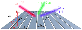
Figure 2: Schematic of a graphene grating with period, $\Lambda$, and width of graphene ribbons, $W$.

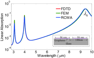
Figure 3: Comparison of the absorption spectra of a graphene grating on a glass substrate, calculated by different methods.

III.2 Linear Results and Discussion

To generate the nonlinear current sources at SH and TH, we first launch in each case a linear simulation to obtain the near-field distribution at FF, for all frequencies of interest. To this end, we calculated the linear optical response of the two graphene gratings using the modified FDTD method described in Section II, the corresponding results being depicted in Fig. 3 (SHG) and Fig. 4 (THG).

These simulations reveal several important results. First, in both cases the absorption spectra possess a series of resonances whose nature can be understood from the profile of the near-field. These field profiles, determined for the first three resonances of the suspended graphene grating, are plotted in Figs. 4b–4d. The strong field confinement of the optical near-field observed at these resonance wavelengths suggests that they are the result of excitation of localized surface plasmons on the graphene ribbons. At these resonances the local field is strongly enhanced, which results in increased optical absorption. This behavior is observed in both gratings, the only difference being that the presence of the dielectric substrate induces a red-shift of the resonance wavelength.

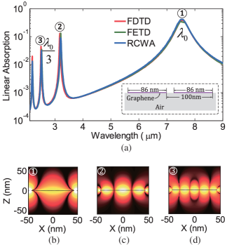
Figure 4: (a) Comparison of the absorption spectra of a suspended graphene grating, calculated by different methods. (b), (c), (d) Spatial distribution of $|E_{x}|$ corresponding to the first three plasmon resonance modes.

A second phenomenon illustrated by Fig. 4 is the existence of a TH double resonance yyn17ptrsa . To be more specific, for the particular values of the grating parameters chosen in this example, there are plasmon resonances both at the fundamental wavelength $\lambda_{0}$ and at the TH wavelength, $\lambda_{0}/3$. Consequently, the near-field at both the FF and TH is resonantly enhanced, such that one expects that the nonlinear currents at the TH are strongly enhanced, too, as per (18a). These nonlinear currents can in turn efficiently radiate into the continuum, which makes these specially engineered optical grating particularly effective nonlinear optical devices for THG yyn17ptrsa .

To verify the accuracy of our modified FDTD method, these two examples have also been simulated by two different numerical methods, namely by OmniSim/FETD (finite-element time-domain) pdsoftware and RCWA wp16prb , both using true 2D models of the graphene. The comparison of the absorption spectra calculated using these three methods shows that there is a very good agreement among the corresponding results, as seen both in Fig. 3 and Fig. 4a. This proves that our modified FDTD method is effective and accurate.

III.3 Nonlinear Results and Discussion

We now consider the nonlinear optical response of the two graphene gratings. Thus, the THG spectrum of the suspended grating is shown in Fig. 5a, together with the spectra obtained using two alternative methods. For completeness, we also present in Figs. 5b–5d the near-field distributions corresponding to the first three peaks in the THG spectrum. Similar to the linear case, the nonlinear spectrum possesses a series of resonances, which can be mapped one-to-one to the resonances of the linear spectra. More exactly, the peaks in THG spectrum occur at exactly a third of the resonance wavelengths of the corresponding absorption peaks. The reason for this is that the absorption and THG intensity are both directly determined by the local near-field at the FF. On the other hand, the field profiles of plasmon resonances are mainly determined by the intrinsic electromagnetic properties of graphene and the structure of the diffraction grating. Consequently, the field profiles at specific resonance wavelengths are generally different from their linear counterparts, which can be readily seen by comparing Fig. 4b and Fig. 5b.

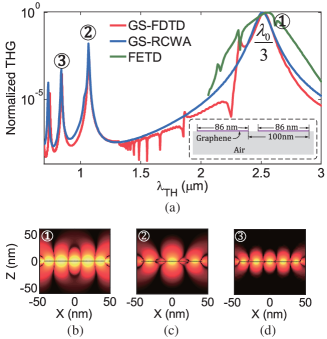
Figure 5: (a) Comparison of THG spectra of suspended graphene grating calculated by three different methods. (b), (c), (d) Spatial distribution of $|E_{x}|$ at TH corresponding to the first three plasmon resonance modes.

As in the linear case, we also compared our results with the predictions of two alternative methods, a GS-RCWA method introduced in wp16prb and OmniSim/FETD pdsoftware , which both incorporate third-order nonlinearities. It should be noted that the latter method does not incorporate the frequency dispersion of the nonlinear susceptibility and models graphene as a slab with thickness of $1.1\text{\,}\mathrm{nm}$ but, on the other hand, it does not rely on the undepleted pump approximation. The results of these simulations suggest that there is a rather good agreement among the predictions of these methods, except for some extra spectral features that are missing in the spectrum calculated using GS-RCWA. A careful inspection of the location of these spectral dips shows that they are due to the excitation of surface plasmons in the grating, which suggests that the GS-RCWA method underestimates the optical loss in graphene.

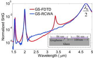
Figure 6: Comparison of SHG from graphene grating on a glass substrate, calculated using two different methods.

To illustrate the versatility of our method in describing different types of nonlinearities, we present now the results pertaining to SHG in the graphene grating placed on a glass substrate and compare them with the predictions of the GS-RCWA method. The conclusions of this analysis, presented in Fig. 6, show that although in this case the predictions of the two methods agree to a lesser extent, the amplitude and width of the plasmon resonances are correctly evaluated by both methods. The differences in the results obtained by using the two methods are explained by the fact that Fourier-series-expansion methods, such as RCWA-type methods, show slow convergence when near-fields are calculated. Although these issues can be circumvented in some cases wgp15jop , in the case of SHG in graphene they still manifest themselves because, unlike the case of THG, which is mainly determined by the dominant field component, $E_{x}$, SHG is chiefly determined by the weak, $E_{z}$ field component. By contrast, grid-based methods, such as FDTD, are effective at the evaluation of the near-field distribution, thus, they are usually more accurate in calculating local nonlinear sources.

Our GS-FDTD method has several other appealing features. First, the GS-FDTD method can be used to model not only periodic structures, but also single scatterers and devices of finite extent. Equally important, in addition to diffraction problems, GS-FDTD method can also be used to study much more complicated nonlinear problems, such as light propagation in a nonlinear medium beyond the paraxial approximation, design of high-Q nonlinear photonic crystal cavities, and radiation from clusters of nonlinear nanoparticles.

IV Conclusion

In conclusion, we have introduced a novel finite-difference time-domain type method suited to accurately study optical structures containing dispersive and nonlinear two-dimensional materials. The dispersive features of these materials are described using a mixture of well-known dispersion models, such as Debye, Drude, and Lorentz models, whereas their frequency-dependent nonlinear response is incorporated in our method via generalized source currents defined by the linear near-field. This general setting allows one to study a multitude of nonlinear processes as one only needs to know the particular dependence of nonlinear currents on the linear near-field. Importantly, since these nonlinear currents are computed in the frequency domain, one avoids the calculation of complex time-domain convolution integrals, thus significantly increasing the computational efficiency of our method. In addition, in order to illustrate the versatility of the method, we employed it to calculate the second- and third-harmonic generation in graphene gratings and showed that good agreement with alternative numerical approaches, such as finite-element method and rigorous coupled-wave analysis, is achieved.

Funding

H2020 European Research Council (ERC) (ERC-2014-CoG-648328).

References

- (1) K. S. Novoselov, A. K. Geim, S. V. Morozov, D. Jiang, Y. Zhang, S. V. Dubonos, I. V. Grigorieva, and A. A. Firsov, “Electric field effect in atomically thin carbon films,” Science 306, 666-669 (2004).
- (2) K. F. Mak, C. Lee, J. Hone, J. Shan, and T. F. Heinz. “Atomically thin : a new direct-gap semiconductor,” Phys. Rev. Lett. 105, 136805 (2010).
- (3) L. Song, L. Ci, H. Lu, P. B. Sorokin, C. Jin, J. Ni, A. G. Kvashnin, D. G. Kvashnin, J. Lou, B. I. Yakobson, and P. M. Ajayan, “Large Scale Growth and Characterization of Atomic Hexagonal Boron Nitride Layers,” Nano Lett. 10, 3209-3215 (2010).
- (4) P. Vogt, P. De Padova, C. Quaresima, J. Avila, E. Frantzeskakis, M. C. Asensio, A. Resta, B. Ealet, and G. Le Lay, “Silicene: compelling experimental evidence for graphenelike two-dimensional silicon,” Phys. Rev. Lett. 108, 155501 (2012).
- (5) Q. H. Wang, K. Kalantar-Zadeh, A. Kis, J. N. Coleman, and M. S. Strano, “Electronics and optoelectronics of two-dimensional transition metal dichalcogenides,” Nature Nanotechnol. 7, 699-712 (2012).
- (6) E. Gibney, “The super materials that could trump graphene,” Nature 522, 274-276 (2015).
- (7) G. R. Bhimanapati, Z. Lin, V. Meunier, Y. Jung, J. Cha, S. Das, D. Xiao et al. “Recent advances in two-dimensional materials beyond graphene,” ACS Nano 9, 11509-11539 (2015).
- (8) A. K. Geim, “Graphene: status and prospects,” Science 324, 1530-1534 (2009).
- (9) F. Schwierz, “Graphene transistors,” Nature Nanotechnol. 5, 487-496 (2010).
- (10) Y. M. Lin, C. Dimitrakopoulos, K. A. Jenkins, D. B. Farmer, H. Y. Chiu, A. Grill, and P. Avouris, “100-GHz transistors from wafer-scale epitaxial graphene,” Science 327, 662-662 (2010).
- (11) B. Radisavljevic, A. Radenovic, J. Brivio, I. V. Giacometti, and A. Kis. “Single-layer MoS2 transistors,” Nature Nanotechnol. 6, 147-150 (2011).
- (12) G. S. Kulkarni, K. Reddy, Z. Zhong, and X. Fan, “Graphene nanoelectronic heterodyne sensor for rapid and sensitive vapour detection,” Nature Commun. 5, (2014).
- (13) H. Li, , Y. Shi, M. H. Chiu, and L. J. Li, “Emerging energy applications of two-dimensional layered transition metal dichalcogenides,” Nano Energy 18, 293-305 (2015).
- (14) M. Zhong, D. Xu, X. Yu, K. Huang, X. Liu, Y. Qu, Y. Xu, and D. Yang, “Interface coupling in graphene/fluorographene heterostructure for high-performance graphene/silicon solar cells,” Nano Energy 28, 12-18 (2016).
- (15) S. Y. Hong, J. I. Dadap, N. Petrone, P. C. Yeh, J. Hone, and R. M. Osgood Jr, “Optical third-harmonic generation in graphene,” Phys. Rev. X 3, 021014 (2013).
- (16) J. L. Cheng, N. Vermeulen, and J. E. Sipe, “Third order optical nonlinearity of graphene,” New J. Phys. 16, 053014 (2014).
- (17) J. D. Cox, I. Silveiro and F. J. G. de Abajo, “Quantum effects in the nonlinear response of graphene plasmons,” ACS Nano 10, 1995-2003 (2016).
- (18) J. W. You, J. You, M. Weismann, and N. C. Panoiu, “Double-resonant enhancement of third-harmonic generation in graphene nanostructures,” Phil. Trans. R. Soc. A 375, 20160313 (2017).
- (19) H. Zhang, S. Virally, Q. Bao, L. K. Ping, S. Massar, N. Godbout, and P. Kockaert, “Z-scan measurement of the nonlinear refractive index of graphene,” Opt. Lett. 37, 1856-1858 (2012).
- (20) N. Kumar, S. Najmaei, Q. Cui, F. Ceballos, P. M. Ajayan, J. Lou, and H. Zhao, “Second harmonic microscopy of monolayer MoS 2,” Phys. Rev. B 87, 161403 (2013).
- (21) L. M. Malard, T. V. Alencar, A. P. M. Barboza, K. F. Mak, and A. M. de Paula, “Observation of intense second harmonic generation from MoS2 atomic crystals,” Phys. Rev. B 87, 201401 (2013).
- (22) G. Wang, X. Marie, I. Gerber, T. Amand, D. Lagarde, L. Bouet, M. Vidal, A. Balocchi, and B. Urbaszek, “Giant enhancement of the optical second-harmonic emission of WSe 2 monolayers by laser excitation at exciton resonances,” Phys. Rev. Lett. 114, 097403 (2015).
- (23) F. Bonaccorso, Z. Sun, T. Hasan, and A. Ferrari, “Graphene photonics and optoelectronics,” Nature Photon. 4, 611-622 (2010).
- (24) F. Xia, T. Mueller, Y. M. Lin, A. Valdes-Garcia, and P. Avouris, “Ultrafast graphene photodetector,” Nature Nanotechnol. 4, 839-843 (2009).
- (25) M. L. Nesterov, J. Bravo Abad, A. Y. Nikitin, F. J. Garcia Vidal, and L. Martin Moreno, “Graphene supports the propagation of subwavelength optical solitons,” Laser Photonics Rev. 7, 7-11 (2013).
- (26) H. Deng, F. Ye, B. A. Malomed, X. Chen, and N. C. Panoiu, “Optically and electrically tunable Dirac points and Zitterbewegung in graphene-based photonic superlattices,” Phys. Rev. B 91, 201402 (2015).
- (27) H. Deng, X. Chen, B. A. Malomed, N. C. Panoiu, and F. Ye “Transverse Anderson localization of light near Dirac points of photonic nanostructures,” Sci. Rep. 5, 15585 (2015).
- (28) R. W. Boyd, Nonlinear Optics, 3rd ed. Academic Press, 2008.
- (29) F. A. Katsriku, B. M. A. Rahman, and K. T. V. Grattan, “Numerical modeling of second harmonic generation in optical waveguides using the finite element method,” IEEE J. Quantum Electron. 33, 1727-1733 (1997).
- (30) T. Fujisawa and M. Koshiba “Finite-Element Mode-Solver for Nonlinear Periodic Optical Waveguides and Its Application to Photonic Crystal Circuits,” J. Light. Technol. 23, 382–387 (2005).
- (31) M. Weismann and N. C. Panoiu, “Theoretical and computational analysis of second- and third-harmonic generation in periodically patterned graphene and transition-metal dichalcogenide monolayers,” Phys. Rev. B 94, 035435 (2016).
- (32) J. Niu, M. Luo, and Q. H. Liu, “Enhancement of graphene’s third-harmonic generation with localized surface plasmon resonance under optical/electro-optic Kerr effects,” J. Opt. Soc. Am. B 33, 615-621 (2016).
- (33) A. Taflove and S. C. Hagness, Computational Electrodynamics: The Finite-Difference Time-Domain Method, 3rd ed. Artech House, 2005.
- (34) R. M. Joseph, and A. Taflove, “FDTD Maxwell’s equations models for nonlinear electrodynamics and optics,” IEEE Trans. Antennas Propag. 45, 364-374 (1997).
- (35) J. H. Greene and A. Taflove, “General vector auxiliary differential equation finite-difference time-domain method for nonlinear optics,” Opt. Express 14, 8305-8310 (2006).
- (36) J. H. Greene and A. Taflove, “Scattering of spatial optical solitons by subwavelength air holes,” IEEE Microwave Wireless Compon. Lett. 17, 760-762 (2007).
- (37) A. Taflove, A. Oskooi, and S. G. Johnson, eds., Advances in FDTD Computational Electrodynamics: Photonics and Nanotechnology, Artech House, 2013.
- (38) V. Van, and S. K. Chaudhuri, “A hybrid implicit-explicit FDTD scheme for nonlinear optical waveguide modeling,” IEEE Trans. Microw. Theory Tech. 47, 540-545 (1999).
- (39) D. M. Sullivan, “Nonlinear FDTD formulations using Z transforms,” IEEE Trans. Microw. Theory Tech. 43, 676-682 (1995).
- (40) G.W. Hanson, “Dyadic Green’s functions and guided surface waves for a surface conductivity model of graphene,” J. Appl. Phys. 103, 064302, (2008).
- (41) D. W. Wang, W. S. Zhao, X. Q. Gu, W. C. Chen, and W. Y. Yin, “Wideband modeling of graphene-based on structures at different temperatures using hybrid FDTD method,” IEEE Trans. Nanotechnol. 14, 250-258 (2015).
- (42) J. W. You, S. R. Tan, and T. J. Cui, “Novel Adaptive Steady-State Criteria for Finite-Difference Time-Domain Method,” IEEE Trans. Microw. Theory Tech. 62, 2849-2858 (2014).
- (43) J. J. Dean, and M. D. Henry, “Second harmonic generation from graphene and graphitic films,” Appl. Phys. Lett. 95, 261910 (2009).
- (44) S. A. Mikhailov, “Theory of the giant plasmon-enhanced second-harmonic generation in graphene and semiconductor two-dimensional electron systems,” Phys. Rev. B 84, 045432 (2011).
- (45) Y. Q. An, J. E. Rowe, D. B. Dougherty, J. U. Lee, and A. C. Diebold, “Optical second-harmonic generation induced by electric current in graphene on Si and SiC substrates,” Phys. Rev. B 89, 115310 (2014).
- (46) J. J. Dean, and M. D. Henry, “Graphene and few-layer graphite probed by second-harmonic generation: Theory and experiment,” Phys. Rev. B 82, 125411 (2010).
- (47) T. J. Constant, S. M. Hornett, D. E. Chang, and E. Hendry, “All-optical generation of surface plasmons in graphene,” Nature Phys. 12, 124-127 (2016).
- (48) J. W. You, J. F. Zhang, W. H. Gu, W. Z. Cui, and T. J. Cui, “Numerical Analysis of Passive Intermodulation Arisen From Nonlinear Contacts in HPMW Devices, ” IEEE Trans. Electromagn. Compat. 60, 1470-1480 (2018).
- (49) C. G. Biris and N. C. Panoiu, “Second harmonic generation in metamaterials based on homogeneous centrosymmetric nanowires,” Phys. Rev. B 81, 195102 (2010).
- (50) J. W. You, H. G. Wang, J. F. Zhang, Y. Li, W. Z. Cui and T. J. Cui, “Highly efficient and adaptive numerical scheme to analyze multipactor in waveguide devices,” IEEE Trans. Electron Devices 62, 1327-1333 (2015).
- (51) J. W. You, H. G. Wang, J. F. Zhang, S. R. Tan, and T. J. Cui, “Accurate numerical method for multipactor analysis in microwave devices,” IEEE Trans. Electron Devices 61, 1546-1552 (2014).
- (52) J. W. You, H.G. Wang,J. F. Zhang, S. R. Tan, and T. J. Cui, “Accurate numerical analysis of nonlinearities caused by multipactor in microwave devices,” IEEE Microw. Wirel. Compon. Lett. 24, 730-732 (2014).
- (53) CST Computer Simulation Technology CST/MWS, https: //www. cst. com/ products /cstmws
- (54) Photon Design Ltd OmniSim/FETD, http:// photond .com /products /omnisim .htm
- (55) M. Weismann, D. F. Gallagher, and N. C. Panoiu, “Accurate near-field calculation in the rigorous coupled-wave analysis method,” J. Opt. 17, 125612 (2015).