Streamlined Variational Inference for

Higher Level Group-Specific Curve Models

By M. Menictas¹, T.H. Nolan¹, D.G. Simpson² and M.P. Wand¹

University of Technology Sydney¹ and University of Illinois²

11th March, 2019

Abstract

A two-level group-specific curve model is such that the mean response of each member of a group is a separate smooth function of a predictor of interest. The three-level extension is such that one grouping variable is nested within another one, and higher level extensions are analogous. Streamlined variational inference for higher level group-specific curve models is a challenging problem. We confront it by systematically working through two-level and then three-level cases and making use of the higher level sparse matrix infrastructure laid down in Nolan & Wand (2018). A motivation is analysis of data from ultrasound technology for which three-level group-specific curve models are appropriate. Whilst extension to the number of levels exceeding three is not covered explicitly, the pattern established by our systematic approach sheds light on what is required for even higher level group-specific curve models.

Keywords: longitudinal data analysis, multilevel models, panel data, mean field variational Bayes.

1 Introduction

We provide explicit algorithms for fitting and approximate Bayesian inference for multilevel models involving, potentially, thousands of noisy curves. The algorithms include covariance parameter estimation and allow for pointwise credible intervals around the fitted curves. Contrast function fitting and inference is also supported by our approach. Both two-level and three-level situations are covered, and a template for even higher level situations is laid down.

Models and methodology for statistical analyses of grouped data for which the basic unit is a noisy curve continues to be an important area of research. A driving force is rapid technological change which is resulting in the generation of curve-type data at fine resolution levels. Examples of such technology include accelerometers (e.g. Goldsmith et al., 2015) personal digital assistants (e.g. Trail et al., 2014) and quantitative ultrasound (e.g. Wirtzfeld et al., 2015). In some applications curve-type data have higher levels of grouping, with groups at one level nested inside other groups. Our focus here is streamlined variational inference for such circumstances.

Some motivating data is shown in Figure 1 from an experiment involving quantitative ultrasound technology. Each curve corresponds to a logarithmically transformed backscatter coefficient over a fine grid of frequency values for tumors in laboratory mice, with exactly one tumor per mouse. The backscatter/frequency curves are grouped according to one of 5 slices of the same tumor, corresponding to probe locations. The slices are grouped according to being from one of 10 tumors. We refer to such data as three-level data with frequency measurements at level 1, slices being the level 2 groups and tumors constituting the level 3 groups. The gist of this article is efficient and flexible variational fitting and inference for such data, that scales well to much larger multilevel data sets. Indeed, our algorithms are linear in the number of groups at both level 2 and level 3. Simulation study results given later in this article show that curve-type data with thousands of groups can be analyzed quickly using our new methodology. Depending on sample sizes and implementation language, fitting times range from a few seconds to a few minutes. In contrast, naïve implementations become infeasible when the number of groups are in the several hundreds due to storage and computational demands.

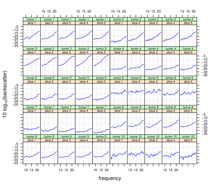
Figure 1: Illustrative three-level curve-type data. The response variable is $10\log_{10}(\mbox{backscatter})$ according to ultrasound technology. Level 1 corresponds to different ultrasound frequencies and matches the horizontal axes in each panel. Level 2 corresponds to different slices of a tumor due to differing probe locations. Level 3 corresponds to different tumors with one tumor for each of $10$ laboratory mice.

We work with a variant of group-specific curve models that at least go back to Donnelly, Laird & Ware (1995). Other contributions of this type include Brumback & Rice (1998), Verbyla et al. (1999), Wang (1998) and Zhang et al. (1998). The specific formulation that we use is that given by Durban et al. (2005) which involves an embedding within the class of linear mixed models (e.g. Robinson, 1991) with low-rank smoothing splines used for flexible function modelling and fitting.

Even though approximate Bayesian variational inference is our overarching goal, we also provide an important parallelism involving classical frequentist inference. Contemporary mixed model software such as nlme() (Pinheiro et al., 2018) and lme4() (Bates et al., 2015) in the R language provide streamlined algorithms for obtaining the best linear unbiased predictions of fixed and random effects in multilevel mixed models with details given in, for example, Pinheiro & Bates (2000). However, the sub-blocks of the covariance matrices required for construction of pointwise confidence interval bands around the estimated curves are not provided by such software. In the variational Bayesian analog, these sub-blocks are required for covariance parameter fitting and inference which, in turn, are needed for curve estimation. A significant contribution of this article is streamlined computation for both the best linear unbiased predictors and its corresponding covariance computation. Similar mathematical results lead to the mean field variational Bayesian inference equivalent. We present explicit ready-to-code algorithms for both two-level and three-level group-specific curve models. Extensions to higher level models could be derived using the blueprint that we establish here. Nevertheless, the algebraic overhead is increasingly burdensome with each increment in the number of levels. It is prudent to treat each multilevel case separately and here we already require several pages to cover two-level and three-level group-specific curve models. To our knowledge, this is the first article to provide streamlined algorithms for fitting three-level group-specific curve models.

Another important aspect of our group-specific curve fitting algorithms is the fact that they make use of the SolveTwoLevelSparseLeastSquares and SolveThreeLevelSparseLeastSquares algorithms developed for ordinary linear mixed models in Nolan et al. (2018). This realization means that the algorithms listed in Sections 2 and 3 are more concise and code-efficient: there is no need to repeat the implementation of these two fundamental algorithms for stable QR-based solving of higher level sparse linear systems. Sections S.11–S.12 of the web-supplement provide details on the SolveThreeLevelSparseLeastSquares and SolveThreeLevelSparseLeastSquares algorithms.

Section 2 deals with the two-level case and the three-level case is covered in Section 3. In Section 4 we provide some assessments concerning the accuracy and speed of the new variational inference algorithms.

2 Two-Level Models

The simplest version of group-specific curve models involves the pairs $(x_{ij},y_{ij})$ where $x_{ij}$ is the $j$th value of the predictor variable within the $i$th group and $y_{ij}$ is the corresponding value of the response variable. We let $m$ denote the number of groups and $n_{i}$ denote the number of predictor/response pairs within the $i$th group. The Gaussian response two-level group specific curve model is

$$y_{ij}=f(x_{ij})+g_{i}(x_{ij})+\varepsilon_{i},\quad\varepsilon_{ij}\stackrel{{\scriptstyle{\tiny\mbox{ind.}}}}{{\sim}}N(0,\sigma_{\varepsilon}^{2}),\quad 1\leq i\leq m,\ 1\leq j\leq n_{i},$$ (1)

where the smooth function $f$ is the global regression mean function and the smooth functions $g_{i}$, $1\leq i\leq m$, allow for flexible group-specific deviations from $f$. As in Durban et al. (2005), we use mixed model-based penalized basis functions to model $f$ and the $g_{i}$. Specifically,

$$f(x) = \beta_{0}+\beta_{1}\,x+\sum_{k=1}^{K_{\mbox{\rm\tiny gbl}}}\,u_{\mbox{\rm\tiny gbl,$k$}}\,z_{\mbox{\rm\tiny gbl,$k$}}(x),\quad u_{\mbox{\rm\tiny gbl,$k$}}\stackrel{{\scriptstyle{\tiny\mbox{ind.}}}}{{\sim}}N(0,\sigma_{\mbox{\rm\tiny gbl}}^{2}),\ \mbox{and}$$

$$g_{i}(x) = u_{\mbox{\rm\tiny lin,$i0$}}+u_{\mbox{\rm\tiny lin,$i1$}}\,x+\sum_{k=1}^{K_{\mbox{\rm\tiny grp}}}\,u_{\mbox{\rm\tiny grp,$ik$}}\,z_{\mbox{\rm\tiny grp,k}}(x),\ \ \left[\begin{array}[]{c}u_{\mbox{\rm\tiny lin,$i0$}}\\[4.30554pt] u_{\mbox{\rm\tiny lin,$i1$}}\end{array}\right]\stackrel{{\scriptstyle{\tiny\mbox{ind.}}}}{{\sim}}N(\boldsymbol{0},\boldsymbol{\Sigma}),\ \ u_{\mbox{\rm\tiny grp,$ik$}}\stackrel{{\scriptstyle{\tiny\mbox{ind.}}}}{{\sim}}N(0,\sigma_{\mbox{\rm\tiny grp}}^{2}),$$

where $\{z_{\mbox{\rm\tiny gbl,$k$}}(\cdot):1\leq k\leq K_{\mbox{\rm\tiny gbl}}\}$ and $\{z_{\mbox{\rm\tiny grp,k}}(\cdot):1\leq k\leq K_{\mbox{\rm\tiny grp}}\}$ are suitable sets of basis functions. Splines and wavelet families are the most common choices for the $z_{\mbox{\rm\tiny gbl,$k$}}(\cdot)$ and $z_{\mbox{\rm\tiny grp,k}}(\cdot)$. In our illustrations and simulation studies we use the canonical cubic O’Sullivan spline basis as described in Section 4 of Wand & Ormerod (2008), which corresponds to a low-rank version of classical smoothing splines (e.g. Wahba, 1990). The variance parameters $\sigma_{\mbox{\rm\tiny gbl}}^{2}$ and $\sigma_{\mbox{\rm\tiny grp}}^{2}$ control the effective degrees of freedom used for the global mean and group-specific deviation functions respectively. Lastly, $\boldsymbol{\Sigma}$ is a $2\times 2$ unstructured covariance matrix for the coefficients of the group-specific linear deviations.

We also use the notation:

$$\boldsymbol{x}_{i}\equiv\left[\begin{array}[]{c}x_{i1}\\ \vdots\\ x_{in_{i}}\end{array}\right]\quad\mbox{and}\quad\boldsymbol{y}_{i}\equiv\left[\begin{array}[]{c}y_{i1}\\ \vdots\\ y_{in_{i}}\end{array}\right]$$

for the vectors of predictors and responses corresponding to the $i$th group. Notation such as $z_{\mbox{\rm\tiny gbl,$1$}}(\boldsymbol{x}_{i})$ denotes the $n_{i}\times 1$ vector containing $z_{\mbox{\rm\tiny gbl,$1$}}(x_{ij})$ values, $1\leq j\leq n_{i}$.

2.1 Best Linear Unbiased Prediction

Model (1) is expressible as a Gaussian response linear mixed model as follows:

$$\boldsymbol{y}|\boldsymbol{u}\sim N(\boldsymbol{X}\boldsymbol{\beta}+\boldsymbol{Z}\,\boldsymbol{u},\sigma_{\varepsilon}^{2}\,\boldsymbol{I}),\quad\boldsymbol{u}\sim N(\boldsymbol{0},\boldsymbol{G}),$$ (3)

where

$$\boldsymbol{X}\equiv\left[\begin{array}[]{c}\boldsymbol{X}_{1}\\ \vdots\\ \boldsymbol{X}_{m}\\ \end{array}\right]\quad\mbox{with}\quad\boldsymbol{X}_{i}\equiv[\boldsymbol{1}\ \boldsymbol{x}_{i}]\quad\mbox{and}\quad\boldsymbol{\beta}\equiv\left[\begin{array}[]{c}\beta_{0}\\[4.30554pt] \beta_{1}\end{array}\right]$$

are the fixed effects design matrix and coefficients, corresponding to the linear component of $f$. The random effects design matrix $\boldsymbol{Z}$ and corresponding random effects vector $\boldsymbol{u}$ are partitioned according to

$$\boldsymbol{Z}=\Big{[}\boldsymbol{Z}_{\mbox{\rm\tiny gbl}}\ \ \mathop{\mbox{\rm blockdiag}}_{1\leq i\leq m}([\boldsymbol{X}_{i}\ \boldsymbol{Z}_{\mbox{\rm\tiny grp,$i$}}])\Big{]}\quad\mbox{and}\quad\boldsymbol{u}=\left[\begin{array}[]{l}\ \ \ \ \ \boldsymbol{u}_{\mbox{\rm\tiny gbl}}\\[4.30554pt] \left[\begin{array}[]{c}\boldsymbol{u}_{\mbox{\rm\tiny lin,$i$}}\\ \boldsymbol{u}_{\mbox{\rm\tiny grp,$i$}}\end{array}\right]_{1\leq i\leq m}\end{array}\right]$$ (4)

where $\boldsymbol{u}_{\mbox{\rm\tiny gbl}}=[u_{\mbox{\rm\tiny gbl,$1$}}\ \ldots\ u_{\mbox{\rm\tiny gbl,$K_{\mbox{\rm\tiny gbl}}$}}]^{T}$ are the coefficients corresponding to the non-linear component of $f$, $\boldsymbol{u}_{\mbox{\rm\tiny lin,$i$}}=[u_{\mbox{\rm\tiny lin,$i0$}}\ u_{\mbox{\rm\tiny lin,$i1$}}]^{T}$ are the coefficients corresponding to the linear component of $g_{i}$ and $\boldsymbol{u}_{\mbox{\rm\tiny grp,$i$}}=[u_{\mbox{\rm\tiny grp,$i1$}}\ \ldots\ u_{\mbox{\rm\tiny grp,$iK_{\mbox{\rm\tiny grp}}$}}]^{T}$ are the coefficients corresponding to the non-linear component of $g_{i}$, $1\leq i\leq m$. In (4), $\boldsymbol{Z}_{\mbox{\rm\tiny gbl}}\equiv\mathop{\mbox{\rm stack}}_{1\leq i\leq m}(\boldsymbol{Z}_{\mbox{\rm\tiny gbl,$i$}})$ and the matrices $\boldsymbol{Z}_{\mbox{\rm\tiny gbl,$i$}}$ and $\boldsymbol{Z}_{\mbox{\rm\tiny grp,$i$}}$, $1\leq i\leq m$, contain, respectively, spline basis functions for the global mean function $f$ and the $i$th group deviation functions $g_{i}$. Specifically,

$$\boldsymbol{Z}_{\mbox{\rm\tiny gbl,$i$}}\equiv[\begin{array}[]{ccc}z_{\mbox{\rm\tiny gbl,$1$}}(\boldsymbol{x}_{i})&\cdots&z_{\mbox{\rm\tiny gbl,$K_{\mbox{\rm\tiny gbl}}$}}(\boldsymbol{x}_{i})\end{array}]\quad\mbox{and}\quad\boldsymbol{Z}_{\mbox{\rm\tiny grp,$i$}}=[\begin{array}[]{ccccc}z_{\mbox{\rm\tiny grp,1}}(\boldsymbol{x}_{i})&\cdots&z_{\mbox{\rm\tiny grp,$K_{\mbox{\rm\tiny grp}}$}}(\boldsymbol{x}_{i})\end{array}]$$

for $1\leq i\leq m$. The corresponding fixed and random effects vectors are

$$\boldsymbol{u}_{\mbox{\rm\tiny gbl}}\sim N(\boldsymbol{0},\sigma_{\mbox{\rm\tiny gbl}}^{2}\boldsymbol{I}_{K_{\mbox{\rm\tiny gbl}}})\quad\mbox{and}\quad\left[\begin{array}[]{c}\boldsymbol{u}_{\mbox{\rm\tiny lin,$i$}}\\[4.30554pt] \boldsymbol{u}_{\mbox{\rm\tiny grp,$i$}}\end{array}\right]\stackrel{{\scriptstyle{\tiny\mbox{ind.}}}}{{\sim}}N\left(\left[\begin{array}[]{c}\boldsymbol{0}\\[4.30554pt] \boldsymbol{0}\end{array}\right],\left[\begin{array}[]{cc}\boldsymbol{\Sigma}&\boldsymbol{O}\\[4.30554pt] \boldsymbol{O}&\sigma_{\mbox{\rm\tiny grp}}^{2}\boldsymbol{I}_{K_{\mbox{\rm\tiny grp}}}\end{array}\right]\right),\quad 1\leq i\leq m.$$

Hence, the full random effects covariance matrix is

$$\boldsymbol{G}=\mbox{\rm Cov}(\boldsymbol{u})=\left[\begin{array}[]{ccc}\sigma_{\mbox{\rm\tiny gbl}}^{2}\boldsymbol{I}_{K_{\mbox{\rm\tiny gbl}}}&\boldsymbol{O}\\[4.30554pt] \boldsymbol{O}&\boldsymbol{I}_{m}\otimes\left[\begin{array}[]{cc}\boldsymbol{\Sigma}&\boldsymbol{O}\\[4.30554pt] \boldsymbol{O}&\sigma_{\mbox{\rm\tiny grp}}^{2}\boldsymbol{I}_{K_{\mbox{\rm\tiny grp}}}\end{array}\right]\end{array}\right].$$ (5)

Next define the matrices

$$\begin{array}[]{c}\boldsymbol{C}\equiv[\boldsymbol{X}\ \boldsymbol{Z}],\quad\boldsymbol{D}_{\mbox{{\bf BLUP}}}\equiv\left[\begin{array}[]{cc}\boldsymbol{O}&\boldsymbol{O}\\[4.30554pt] \boldsymbol{O}&\boldsymbol{G}^{-1}\end{array}\right]\quad\mbox{and}\quad\boldsymbol{R}_{\mbox{{\bf BLUP}}}\equiv\sigma_{\varepsilon}^{2}\boldsymbol{I}.\end{array}$$ (6)

The best linear unbiased predictor of $[\boldsymbol{\beta}\ \boldsymbol{u}]^{T}$ and corresponding covariance matrix are

$${\begin{array}[]{rcl}\left[\begin{array}[]{c}{\widehat{\boldsymbol{\beta}}}\\ {\widehat{\boldsymbol{u}}}\end{array}\right]&=&(\boldsymbol{C}^{T}\boldsymbol{R}_{\mbox{{\bf BLUP}}}^{-1}\boldsymbol{C}+\boldsymbol{D}_{\mbox{{\bf BLUP}}})^{-1}\boldsymbol{C}^{T}\boldsymbol{R}_{\mbox{{\bf BLUP}}}^{-1}\boldsymbol{y}\\[12.91663pt] \mbox{and}\quad\mbox{Cov}\left(\left[\begin{array}[]{c}{\widehat{\boldsymbol{\beta}}}\\ {\widehat{\boldsymbol{u}}}-\boldsymbol{u}\end{array}\right]\right)&=&(\boldsymbol{C}^{T}\boldsymbol{R}_{\mbox{{\bf BLUP}}}^{-1}\boldsymbol{C}+\boldsymbol{D}_{\mbox{{\bf BLUP}}})^{-1}.\end{array}}$$ (7)

This covariance matrix grows quadratically in $m$, so its storage becomes infeasible for large numbers of groups. However, only the following sub-blocks are required for adding pointwise confidence intervals to curve estimates:

$${\begin{array}[]{rcl}\mbox{\rm Cov}\left(\left[\begin{array}[]{c}{\widehat{\boldsymbol{\beta}}}\\ {\widehat{\boldsymbol{u}}}_{\mbox{\rm\tiny gbl}}-\boldsymbol{u}_{\mbox{\rm\tiny gbl}}\end{array}\right]\right)&=&\mbox{top left-hand $(2+K_{\mbox{\rm\tiny gbl}})\times(2+K_{\mbox{\rm\tiny gbl}})$ }\\[0.0pt] &&\mbox{sub-block of $(\boldsymbol{C}^{T}\boldsymbol{R}_{\mbox{{\bf BLUP}}}^{-1}\boldsymbol{C}+\boldsymbol{D}_{\mbox{{\bf BLUP}}})^{-1}$},\\[17.22217pt] \mbox{\rm Cov}\left(\left[\begin{array}[]{c}{\widehat{\boldsymbol{u}}}_{\mbox{\rm\tiny lin,$i$}}-\boldsymbol{u}_{\mbox{\rm\tiny lin,$i$}}\\[4.30554pt] {\widehat{\boldsymbol{u}}}_{\mbox{\rm\tiny grp,$i$}}-\boldsymbol{u}_{\mbox{\rm\tiny grp,$i$}}\end{array}\right]\right)&=&\mbox{subsequent $(2+K_{\mbox{\rm\tiny grp}})\times(2+K_{\mbox{\rm\tiny grp}})$ diagonal}\\[0.0pt] &&\mbox{sub-blocks of $(\boldsymbol{C}^{T}\boldsymbol{R}_{\mbox{{\bf BLUP}}}^{-1}\boldsymbol{C}+\boldsymbol{D}_{\mbox{{\bf BLUP}}})^{-1}$}\\[4.30554pt] &&\mbox{below $\mbox{\rm Cov}\left(\left[\begin{array}[]{c}{\widehat{\boldsymbol{\beta}}}\\ {\widehat{\boldsymbol{u}}}_{\mbox{\rm\tiny gbl}}-\boldsymbol{u}_{\mbox{\rm\tiny gbl}}\end{array}\right]\right)$,\ $1\leq i\leq m$, and}\\[8.61108pt] E\left\{\left[\begin{array}[]{c}{\widehat{\boldsymbol{\beta}}}\\ {\widehat{\boldsymbol{u}}}_{\mbox{\rm\tiny gbl}}-\boldsymbol{u}_{\mbox{\rm\tiny gbl}}\end{array}\right]\left[\begin{array}[]{c}{\widehat{\boldsymbol{u}}}_{\mbox{\rm\tiny lin,$i$}}-\boldsymbol{u}_{\mbox{\rm\tiny lin,$i$}}\\[4.30554pt] {\widehat{\boldsymbol{u}}}_{\mbox{\rm\tiny grp,$i$}}-\boldsymbol{u}_{\mbox{\rm\tiny grp,$i$}}\end{array}\right]^{T}\right\}&=&\mbox{subsequent $(2+K_{\mbox{\rm\tiny gbl}})\times(2+K_{\mbox{\rm\tiny grp}})$ sub-blocks}\\[0.0pt] &&\mbox{of $(\boldsymbol{C}^{T}\boldsymbol{R}_{\mbox{{\bf BLUP}}}^{-1}\boldsymbol{C}+\boldsymbol{D}_{\mbox{{\bf BLUP}}})^{-1}$ to the right of}\\[4.30554pt] &&\mbox{$\mbox{\rm Cov}\left(\left[\begin{array}[]{c}{\widehat{\boldsymbol{\beta}}}\\ {\widehat{\boldsymbol{u}}}_{\mbox{\rm\tiny gbl}}-\boldsymbol{u}_{\mbox{\rm\tiny gbl}}\end{array}\right]\right)$,\ $1\leq i\leq m$.}\end{array}}$$ (8)

As in Nolan, Menictas & Wand (2019), we define the generic two-level sparse matrix to be determination of the vector $\boldsymbol{x}$ which minimizes the least squares criterion

$$\|\boldsymbol{b}-\boldsymbol{B}\boldsymbol{x}\|^{2}\quad\mbox{where $\|\boldsymbol{v}\|^{2}\equiv\boldsymbol{v}^{T}\boldsymbol{v}$ for any column vector $\boldsymbol{v}$,}$$ (9)

with $\boldsymbol{B}$ having the two-level sparse form

$$\boldsymbol{B}\equiv\left[\begin{array}[]{c|c|c|c|c}\boldsymbol{B}_{1}&\overset{\ \mbox{{$\bullet$}}}{\boldsymbol{B}}_{1}&\boldsymbol{O}&\cdots&\boldsymbol{O}\\ \hline\cr\boldsymbol{B}_{2}&\boldsymbol{O}&\overset{\ \mbox{{$\bullet$}}}{\boldsymbol{B}}_{2}&\cdots&\boldsymbol{O}\\ \hline\cr\vdots&\vdots&\vdots&\ddots&\vdots\\ \hline\cr\boldsymbol{B}_{m}&\boldsymbol{O}&\boldsymbol{O}&\cdots&\overset{\ \mbox{{$\bullet$}}}{\boldsymbol{B}}_{m}\end{array}\right]\quad\mbox{and $\boldsymbol{b}$ partitioned according to}\quad\boldsymbol{b}\equiv\left[\begin{array}[]{c}\boldsymbol{b}_{1}\\ \hline\cr\boldsymbol{b}_{2}\\ \hline\cr\vdots\\ \hline\cr\boldsymbol{b}_{m}\\ \end{array}\right].$$ (10)

In (10), for any $1\leq i\leq m$, the matrices $\boldsymbol{B}_{i}$, $\overset{\ \mbox{{$\bullet$}}}{\boldsymbol{B}}_{i}$ and $\boldsymbol{b}_{i}$ each have the same number of rows. The numbers of columns in $\boldsymbol{B}_{i}$ and $\overset{\ \mbox{{$\bullet$}}}{\boldsymbol{B}}_{i}$ are arbitrary whereas the $\boldsymbol{b}_{i}$ are column vectors. In addition to solving for $\boldsymbol{x}$, the sub-blocks of $(\boldsymbol{B}^{T}\boldsymbol{B})^{-1}$ corresponding to the non-sparse regions of $\boldsymbol{B}^{T}\boldsymbol{B}$ are included in our definition of a two-level sparse matrix least squares problem. Algorithm 2 of Nolan et al. (2018) provides a stable and efficient solution to this problem and labels it the SolveTwoLevelSparseLeastSquares algorithm. Section S.11 of the web-supplement contains details regarding this algorithm. In Nolan et al. (2018) we used SolveTwoLevelSparseLeastSquares for fitting two-level linear mixed models. However, precisely the same algorithm can be used for fitting two-level group-specific curve models because of:

Result 1.

Computation of $[{\widehat{\boldsymbol{\beta}}}^{T}\ \ {\widehat{\boldsymbol{u}}}^{T}]^{T}$ and each of the sub-blocks of $\mbox{\rm Cov}([{\widehat{\boldsymbol{\beta}}}^{T}\ \ ({\widehat{\boldsymbol{u}}}-\boldsymbol{u})^{T}]^{T})$ listed in (8) are expressible as solutions to the two-level sparse matrix least squares problem:

$$\left\|\boldsymbol{b}-\boldsymbol{B}\left[\begin{array}[]{c}\boldsymbol{\beta}\\ \boldsymbol{u}\end{array}\right]\right\|^{2}$$

where the non-zero sub-blocks $\boldsymbol{B}$ and $\boldsymbol{b}$, according to the notation in (10), are for $1\leq i\leq m$:

$$\boldsymbol{b}_{i}\equiv\left[\begin{array}[]{c}\sigma_{\varepsilon}^{-1}\boldsymbol{y}_{i}\\[4.30554pt] \boldsymbol{0}\\[4.30554pt] \boldsymbol{0}\\[4.30554pt] \boldsymbol{0}\\[4.30554pt] \end{array}\right],\quad\boldsymbol{B}_{i}\equiv\left[\begin{array}[]{cc}\sigma_{\varepsilon}^{-1}\boldsymbol{X}_{i}&\sigma_{\varepsilon}^{-1}\boldsymbol{Z}_{\mbox{\rm\tiny gbl,$i$}}\\[4.30554pt] \boldsymbol{O}&m^{-1/2}\sigma_{\mbox{\rm\tiny gbl}}^{-1}\boldsymbol{I}_{K_{\mbox{\rm\tiny gbl}}}\\[4.30554pt] \boldsymbol{O}&\boldsymbol{O}\\[4.30554pt] \boldsymbol{O}&\boldsymbol{O}\\[4.30554pt] \end{array}\right]\quad\mbox{and}\quad\overset{\ \mbox{{$\bullet$}}}{\boldsymbol{B}}_{i}\equiv\left[\begin{array}[]{cc}\sigma_{\varepsilon}^{-1}\boldsymbol{X}_{i}&\sigma_{\varepsilon}^{-1}\boldsymbol{Z}_{\mbox{\rm\tiny grp,$i$}}\\[4.30554pt] \boldsymbol{O}&\boldsymbol{O}\\[4.30554pt] \boldsymbol{\Sigma}^{-1/2}&\boldsymbol{O}\\[4.30554pt] \boldsymbol{O}&\sigma_{\mbox{\rm\tiny grp}}^{-1}\boldsymbol{I}_{K_{\mbox{\rm\tiny grp}}}\end{array}\right]$$

with each of these matrices having ${\tilde{n}}_{i}=n_{i}+K_{\mbox{\rm\tiny gbl}}+2+K_{\mbox{\rm\tiny grp}}$ rows and with $\boldsymbol{B}_{i}$ having $p=2+K_{\mbox{\rm\tiny gbl}}$ columns and $\overset{\ \mbox{{$\bullet$}}}{\boldsymbol{B}}_{i}$ having $q=2+K_{\mbox{\rm\tiny grp}}$ columns. The solutions are

$$\left[\begin{array}[]{c}{\widehat{\boldsymbol{\beta}}}\\ {\widehat{\boldsymbol{u}}}_{\mbox{\rm\tiny gbl}}\end{array}\right]=\boldsymbol{x}_{1},\quad\mbox{\rm Cov}\left(\left[\begin{array}[]{c}{\widehat{\boldsymbol{\beta}}}\\ {\widehat{\boldsymbol{u}}}_{\mbox{\rm\tiny gbl}}-\boldsymbol{u}_{\mbox{\rm\tiny gbl}}\end{array}\right]\right)=\boldsymbol{A}^{11}$$

and

$$\left[\begin{array}[]{c}{\widehat{\boldsymbol{u}}}_{\mbox{\rm\tiny lin,$i$}}\\[4.30554pt] {\widehat{\boldsymbol{u}}}_{\mbox{\rm\tiny grp,$i$}}\end{array}\right]=\boldsymbol{x}_{2,i},\quad E\left\{\left[\begin{array}[]{c}{\widehat{\boldsymbol{\beta}}}\\ {\widehat{\boldsymbol{u}}}_{\mbox{\rm\tiny gbl}}-\boldsymbol{u}_{\mbox{\rm\tiny gbl}}\end{array}\right]\left[\begin{array}[]{c}{\widehat{\boldsymbol{u}}}_{\mbox{\rm\tiny lin,$i$}}-\boldsymbol{u}_{\mbox{\rm\tiny lin,$i$}}\\[4.30554pt] {\widehat{\boldsymbol{u}}}_{\mbox{\rm\tiny grp,$i$}}-\boldsymbol{u}_{\mbox{\rm\tiny grp,$i$}}\end{array}\right]^{T}\right\}=\boldsymbol{A}^{12,i},$$

$$\mbox{\rm Cov}\left(\left[\begin{array}[]{c}{\widehat{\boldsymbol{u}}}_{\mbox{\rm\tiny lin,$i$}}-\boldsymbol{u}_{\mbox{\rm\tiny lin,$i$}}\\[4.30554pt] {\widehat{\boldsymbol{u}}}_{\mbox{\rm\tiny grp,$i$}}-\boldsymbol{u}_{\mbox{\rm\tiny grp,$i$}}\end{array}\right]\right)=\boldsymbol{A}^{22,i},\ \ 1\leq i\leq m.$$

A derivation of Result 1 is given in Section S.1 of the web-supplement. Algorithm 1 encapsulates streamlined best linear unbiased prediction computation together with coefficient covariance matrix sub-blocks of interest.

• Inputs: $\boldsymbol{y}_{i}(n_{i}\times 1),\ \boldsymbol{X}_{i}(n_{i}\times 2),\ \boldsymbol{Z}_{\mbox{\rm\tiny gbl,$i$}}(n_{i}\times K_{\mbox{\rm\tiny gbl}}),\ \boldsymbol{Z}_{\mbox{\rm\tiny grp,$i$}}(n_{i}\times K_{\mbox{\rm\tiny grp}}),\ 1\leq i\leq m$;  $\sigma_{\varepsilon}^{2},\sigma_{\mbox{\rm\tiny gbl}}^{2},\sigma_{\mbox{\rm\tiny grp}}^{2}>0$,
                 $\boldsymbol{\Sigma}(q\times q),\mbox{symmetric and positive definite.}$

• For $i=1,\ldots,m$:

  • $\begin{array}[]{l}\boldsymbol{b}_{i}\longleftarrow\left[\begin{array}[]{c}\sigma_{\varepsilon}^{-1}\boldsymbol{y}_{i}\\[3.87498pt] \boldsymbol{0}\\[3.87498pt] \boldsymbol{0}\\[3.87498pt] \boldsymbol{0}\\[3.87498pt] \end{array}\right],\ \boldsymbol{B}_{i}\longleftarrow\left[\begin{array}[]{cc}\sigma_{\varepsilon}^{-1}\boldsymbol{X}_{i}&\sigma_{\varepsilon}^{-1}\boldsymbol{Z}_{\mbox{\rm\tiny gbl,$i$}}\\[3.87498pt] \boldsymbol{O}&m^{-1/2}\sigma_{\mbox{\rm\tiny gbl}}^{-1}\boldsymbol{I}_{K_{\mbox{\rm\tiny gbl}}}\\[3.87498pt] \boldsymbol{O}&\boldsymbol{O}\\[3.87498pt] \boldsymbol{O}&\boldsymbol{O}\\[3.87498pt] \end{array}\right],\end{array}$

  • $\begin{array}[]{l}\overset{\ \mbox{{$\bullet$}}}{\boldsymbol{B}}_{i}\longleftarrow\left[\begin{array}[]{cc}\sigma_{\varepsilon}^{-1}\boldsymbol{X}_{i}&\sigma_{\varepsilon}^{-1}\boldsymbol{Z}_{\mbox{\rm\tiny grp,$i$}}\\[3.87498pt] \boldsymbol{O}&\boldsymbol{O}\\[3.87498pt] \boldsymbol{\Sigma}^{-1/2}&\boldsymbol{O}\\[3.87498pt] \boldsymbol{O}&\sigma_{\mbox{\rm\tiny grp}}^{-1}\boldsymbol{I}_{K_{\mbox{\rm\tiny grp}}}\end{array}\right]\end{array}$

• ${\mathcal{S}}_{1}\longleftarrow\textsc{\footnotesize SolveTwoLevelSparseLeastSquares}\Big{(}\big{\{}(\boldsymbol{b}_{i},\boldsymbol{B}_{i},\overset{\ \mbox{{$\bullet$}}}{\boldsymbol{B}}_{i}):1\leq i\leq m\big{\}}\Big{)}$

• $\left[\begin{array}[]{c}{\widehat{\boldsymbol{\beta}}}\\ {\widehat{\boldsymbol{u}}}_{\mbox{\rm\tiny gbl}}\end{array}\right]\longleftarrow\mbox{$\boldsymbol{x}_{1}$ component of ${\mathcal{S}}_{1}$}$   ;   $\mbox{\rm Cov}\left(\left[\begin{array}[]{c}{\widehat{\boldsymbol{\beta}}}\\ {\widehat{\boldsymbol{u}}}_{\mbox{\rm\tiny gbl}}-\boldsymbol{u}_{\mbox{\rm\tiny gbl}}\end{array}\right]\right)\longleftarrow\mbox{$\boldsymbol{A}^{11}$ component of ${\mathcal{S}}_{1}$}$

• For $i=1,\ldots,m$:

  • $\left[\begin{array}[]{c}{\widehat{\boldsymbol{u}}}_{\mbox{\rm\tiny lin,$i$}}\\[3.87498pt] {\widehat{\boldsymbol{u}}}_{\mbox{\rm\tiny grp,$i$}}\end{array}\right]\longleftarrow\mbox{$\boldsymbol{x}_{2,i}$ component of ${\mathcal{S}}_{1}$}$

  • $\mbox{\rm Cov}\left(\left[\begin{array}[]{c}{\widehat{\boldsymbol{u}}}_{\mbox{\rm\tiny lin,$i$}}-\boldsymbol{u}_{\mbox{\rm\tiny lin,$i$}}\\[3.87498pt] {\widehat{\boldsymbol{u}}}_{\mbox{\rm\tiny grp,$i$}}-\boldsymbol{u}_{\mbox{\rm\tiny grp,$i$}}\end{array}\right]\right)\longleftarrow\mbox{$\boldsymbol{A}^{22,i}$ component of ${\mathcal{S}}_{1}$}$

  • $E\left\{\left[\begin{array}[]{c}{\widehat{\boldsymbol{\beta}}}\\ {\widehat{\boldsymbol{u}}}_{\mbox{\rm\tiny gbl}}-\boldsymbol{u}_{\mbox{\rm\tiny gbl}}\end{array}\right]\left[\begin{array}[]{c}{\widehat{\boldsymbol{u}}}_{\mbox{\rm\tiny lin,$i$}}-\boldsymbol{u}_{\mbox{\rm\tiny lin,$i$}}\\[3.87498pt] {\widehat{\boldsymbol{u}}}_{\mbox{\rm\tiny grp,$i$}}-\boldsymbol{u}_{\mbox{\rm\tiny grp,$i$}}\end{array}\right]^{T}\right\}\longleftarrow\mbox{$\boldsymbol{A}^{12,i}$ component of ${\mathcal{S}}_{1}$}$

• Output:

  $$\begin{array}[]{c}\Bigg{(}\left[\begin{array}[]{c}{\widehat{\boldsymbol{\beta}}}\\ {\widehat{\boldsymbol{u}}}_{\mbox{\rm\tiny gbl}}\end{array}\right],\ \mbox{\rm Cov}\left(\left[\begin{array}[]{c}{\widehat{\boldsymbol{\beta}}}\\ {\widehat{\boldsymbol{u}}}_{\mbox{\rm\tiny gbl}}-\boldsymbol{u}_{\mbox{\rm\tiny gbl}}\end{array}\right]\right),\Bigg{\{}\Bigg{(}\left[\begin{array}[]{c}{\widehat{\boldsymbol{u}}}_{\mbox{\rm\tiny lin,$i$}}\\[3.87498pt] {\widehat{\boldsymbol{u}}}_{\mbox{\rm\tiny grp,$i$}}\end{array}\right],\,\mbox{\rm Cov}\left(\left[\begin{array}[]{c}{\widehat{\boldsymbol{u}}}_{\mbox{\rm\tiny lin,$i$}}-\boldsymbol{u}_{\mbox{\rm\tiny lin,$i$}}\\[3.87498pt] {\widehat{\boldsymbol{u}}}_{\mbox{\rm\tiny grp,$i$}}-\boldsymbol{u}_{\mbox{\rm\tiny grp,$i$}}\end{array}\right]\right),\\[7.74997pt] E\left\{\left[\begin{array}[]{c}{\widehat{\boldsymbol{\beta}}}\\ {\widehat{\boldsymbol{u}}}_{\mbox{\rm\tiny gbl}}-\boldsymbol{u}_{\mbox{\rm\tiny gbl}}\end{array}\right]\left[\begin{array}[]{c}{\widehat{\boldsymbol{u}}}_{\mbox{\rm\tiny lin,$i$}}-\boldsymbol{u}_{\mbox{\rm\tiny lin,$i$}}\\[3.87498pt] {\widehat{\boldsymbol{u}}}_{\mbox{\rm\tiny grp,$i$}}-\boldsymbol{u}_{\mbox{\rm\tiny grp,$i$}}\end{array}\right]^{T}\right\}\Bigg{)}:\ 1\leq i\leq m\Bigg{\}}\Bigg{)}\end{array}$$

Algorithm 1 Streamlined algorithm for obtaining best linear unbiased predictions and corresponding covariance matrix components for the two-level group specific curves model.

2.2 Mean Field Variational Bayes

We now consider the following Bayesian extension of (3) and (5):

$$\begin{array}[]{c}\boldsymbol{y}|\boldsymbol{\beta},\boldsymbol{u},\sigma_{\varepsilon}^{2}\sim N(\boldsymbol{X}\boldsymbol{\beta}+\boldsymbol{Z}\,\boldsymbol{u},\sigma_{\varepsilon}^{2}\,\boldsymbol{I}),\quad\boldsymbol{u}|\sigma_{\mbox{\rm\tiny gbl}}^{2},\sigma_{\mbox{\rm\tiny grp}}^{2},\boldsymbol{\Sigma}\sim N(\boldsymbol{0},\boldsymbol{G}),\quad\mbox{$\boldsymbol{G}$ as defined in (\ref{eq:Gdefn}),}\\[4.30554pt] \boldsymbol{\beta}\sim N(\boldsymbol{\mu}_{\boldsymbol{\beta}},\boldsymbol{\Sigma}_{\boldsymbol{\beta}}),\quad\sigma_{\varepsilon}^{2}|a_{\varepsilon}\sim\mbox{Inverse-$\chi^{2}$}(\nu_{\varepsilon},1/a_{\varepsilon}),\quad a_{\varepsilon}\sim\mbox{Inverse-$\chi^{2}$}(1,1/(\nu_{\varepsilon}s_{\varepsilon}^{2})),\\[8.61108pt] \quad\sigma_{\mbox{\rm\tiny gbl}}^{2}|a_{\mbox{\rm\tiny gbl}}\sim\mbox{Inverse-$\chi^{2}$}(\nu_{\mbox{\rm\tiny gbl}},1/a_{\mbox{\rm\tiny gbl}}),\quad a_{\mbox{\rm\tiny gbl}}\sim\mbox{Inverse-$\chi^{2}$}(1,1/(\nu_{\mbox{\rm\tiny gbl}}s_{\mbox{\rm\tiny gbl}}^{2})),\\[8.61108pt] \quad\sigma_{\mbox{\rm\tiny grp}}^{2}|a_{\mbox{\rm\tiny grp}}\sim\mbox{Inverse-$\chi^{2}$}(\nu_{\mbox{\rm\tiny grp}},1/a_{\mbox{\rm\tiny grp}}),\quad a_{\mbox{\rm\tiny grp}}\sim\mbox{Inverse-$\chi^{2}$}(1,1/(\nu_{\mbox{\rm\tiny grp}}s_{\mbox{\rm\tiny grp}}^{2})),\\[8.61108pt] \boldsymbol{\Sigma}|\boldsymbol{A}_{\mbox{\rm\tiny$\boldsymbol{\Sigma}$}}\sim\mbox{Inverse-G-Wishart}\big{(}G_{\mbox{\rm\tiny full}},\nu_{\mbox{\rm\tiny{$\boldsymbol{\Sigma}$}}}+2,\boldsymbol{A}_{\mbox{\rm\tiny$\boldsymbol{\Sigma}$}}^{-1}\big{)},\\[8.61108pt] \boldsymbol{A}_{\mbox{\rm\tiny$\boldsymbol{\Sigma}$}}\sim\mbox{Inverse-G-Wishart}(G_{\mbox{\rm\tiny diag}},1,\boldsymbol{\Lambda}_{\boldsymbol{A}_{\mbox{\rm\tiny$\boldsymbol{\Sigma}$}}}),\quad\boldsymbol{\Lambda}_{\boldsymbol{A}_{\mbox{\rm\tiny$\boldsymbol{\Sigma}$}}}\equiv\{\nu_{\mbox{\rm\tiny{$\boldsymbol{\Sigma}$}}}\mbox{diag}(s_{\mbox{\rm\tiny{$\boldsymbol{\Sigma},1$}}}^{2},s_{\mbox{\rm\tiny{$\boldsymbol{\Sigma},2$}}}^{2})\}^{-1}.\end{array}$$ (11)

Here the $2\times 1$ vector $\boldsymbol{\mu}_{\boldsymbol{\beta}}$ and $2\times 2$ symmetric positive definite matrix $\boldsymbol{\Sigma}_{\boldsymbol{\beta}}$ are hyperparameters corresponding to the prior distribution on $\boldsymbol{\beta}$ and

$$\nu_{\varepsilon},s_{\varepsilon},\nu_{\mbox{\rm\tiny gbl}},s_{\mbox{\rm\tiny gbl}},\nu_{\mbox{\rm\tiny grp}},s_{\mbox{\rm\tiny grp}},\nu_{\mbox{\rm\tiny{$\boldsymbol{\Sigma}$}}},s_{\mbox{\rm\tiny{$\boldsymbol{\Sigma},1$}}},s_{\mbox{\rm\tiny{$\boldsymbol{\Sigma},2$}}}>0$$

are hyperparameters for the variance and covariance matrix parameters. Details on the Inverse G-Wishart distribution, and the Inverse-$\chi^{2}$ special case, are given in Section S.3 of the web-supplement. The auxiliary variable $a_{\varepsilon}$ is defined so that $\sigma_{\varepsilon}$ has a Half-$t$ distribution with degrees of freedom parameter $\nu_{\varepsilon}$ and scale parameter $s_{\varepsilon}$, with larger values of $s_{\varepsilon}$ corresponding to greater noninformativity. Analogous comments apply to the other standard deviation parameters. Setting $\nu_{\mbox{\rm\tiny{$\boldsymbol{\Sigma}$}}}=2$ leads to the correlation parameter in $\boldsymbol{\Sigma}$ having a Uniform distribution on $(-1,1)$ (Huang & Wand, 2013).

Throughout this article we use $\mathfrak{p}$ generically to denote a density function corresponding to random quantities in Bayesian models such as (11). For example, $\mathfrak{p}(\boldsymbol{\beta})$ denotes the prior density function of $\boldsymbol{\beta}$ and $\mathfrak{p}(\boldsymbol{u}|\sigma_{\mbox{\rm\tiny gbl}}^{2},\sigma_{\mbox{\rm\tiny grp}}^{2},\boldsymbol{\Sigma})$ denotes the density function of $\boldsymbol{u}$ conditional on $(\sigma_{\mbox{\rm\tiny gbl}}^{2},\sigma_{\mbox{\rm\tiny grp}}^{2},\boldsymbol{\Sigma})$. Now consider the following mean field restriction on the joint posterior density function of all parameters in (11):

$$\mathfrak{p}(\boldsymbol{\beta},\boldsymbol{u},a_{\varepsilon},a_{\mbox{\rm\tiny gbl}},a_{\mbox{\rm\tiny grp}},\boldsymbol{A}_{\mbox{\rm\tiny$\boldsymbol{\Sigma}$}},\sigma_{\varepsilon}^{2},\sigma_{\mbox{\rm\tiny gbl}}^{2},\sigma_{\mbox{\rm\tiny grp}}^{2},\boldsymbol{\Sigma}|\boldsymbol{y})\approx\mathfrak{q}(\boldsymbol{\beta},\boldsymbol{u},a_{\varepsilon},a_{\mbox{\rm\tiny gbl}},a_{\mbox{\rm\tiny grp}},\boldsymbol{A}_{\mbox{\rm\tiny$\boldsymbol{\Sigma}$}})\,\mathfrak{q}(\sigma_{\varepsilon}^{2},\sigma_{\mbox{\rm\tiny gbl}}^{2},\sigma_{\mbox{\rm\tiny grp}}^{2},\boldsymbol{\Sigma}).$$ (12)

Here, generically, each $\mathfrak{q}$ denotes an approximate posterior density function of the random vector indicated by its argument according to the mean field restriction (12). Then application of the minimum Kullback-Leibler divergence equations (e.g. equation (10.9) of Bishop, 2006) leads to the optimal $\mathfrak{q}$-density functions for the parameters of interest being as follows:

$$\begin{array}[]{c}\begin{array}[]{ll}&\mathfrak{q}^{*}(\boldsymbol{\beta},\boldsymbol{u})\ \mbox{has a $N\big{(}\boldsymbol{\mu}_{\mathfrak{q}(\boldsymbol{\beta},\boldsymbol{u})},\boldsymbol{\Sigma}_{\mathfrak{q}(\boldsymbol{\beta},\boldsymbol{u})}\big{)}$ distribution,}\\[6.45831pt] &\mathfrak{q}^{*}(\sigma_{\varepsilon}^{2})\ \mbox{has an $\mbox{Inverse-$\chi^{2}$}\big{(}\xi_{\mathfrak{q}(\sigma_{\varepsilon}^{2})},\lambda_{\mathfrak{q}(\sigma_{\varepsilon}^{2})}\big{)}$ distribution,}\\[6.45831pt] &\mathfrak{q}^{*}(\sigma_{\mbox{\rm\tiny gbl}}^{2})\ \mbox{has an $\mbox{Inverse-$\chi^{2}$}\big{(}\xi_{\mathfrak{q}(\sigma_{\mbox{\rm\tiny gbl}}^{2})},\lambda_{\mathfrak{q}(\sigma_{\mbox{\rm\tiny gbl}}^{2})}\big{)}$ distribution,}\\[6.45831pt] &\mathfrak{q}^{*}(\sigma_{\mbox{\rm\tiny grp}}^{2})\ \mbox{has an $\mbox{Inverse-$\chi^{2}$}\big{(}\xi_{\mathfrak{q}(\sigma_{\mbox{\rm\tiny grp}}^{2})},\lambda_{\mathfrak{q}(\sigma_{\mbox{\rm\tiny grp}}^{2})}\big{)}$ distribution}\\[6.45831pt] \mbox{and}&\mathfrak{q}^{*}(\boldsymbol{\Sigma})\ \mbox{has an $\mbox{Inverse-G-Wishart}(G_{\mbox{\rm\tiny full}},\xi_{\mathfrak{q}(\boldsymbol{\Sigma})},\boldsymbol{\Lambda}_{\mathfrak{q}(\boldsymbol{\Sigma})})$ distribution.}\\ \end{array}\end{array}$$

The optimal $\mathfrak{q}$-density parameters are determined via an iterative coordinate ascent algorithm, with details given in Section S.5 of this article’s web-supplement. The stopping criterion is based on the variational lower bound on the marginal likelihood (e.g. Bishop, 2006; Section 10.2.2) and denoted $\underline{\mathfrak{p}}(\boldsymbol{y};\mathfrak{q})$. Its logarithmic form and derivation are given in Section S.6 of the web-supplement.

Note that updates for $\boldsymbol{\mu}_{\mathfrak{q}(\boldsymbol{\beta},\boldsymbol{u})}$ and $\boldsymbol{\Sigma}_{\mathfrak{q}(\boldsymbol{\beta},\boldsymbol{u})}$ may be written

$$\boldsymbol{\mu}_{\mathfrak{q}(\boldsymbol{\beta},\boldsymbol{u})}\leftarrow(\boldsymbol{C}^{T}\boldsymbol{R}_{\mbox{{\bf MFVB}}}^{-1}\boldsymbol{C}+\boldsymbol{D}_{\mbox{{\bf MFVB}}})^{-1}(\boldsymbol{C}^{T}\boldsymbol{R}_{\mbox{{\bf MFVB}}}^{-1}\boldsymbol{y}+\boldsymbol{o}_{\mbox{{\bf MFVB}}})\quad\mbox{and}\quad\boldsymbol{\Sigma}_{\mathfrak{q}(\boldsymbol{\beta},\boldsymbol{u})}\leftarrow(\boldsymbol{C}^{T}\boldsymbol{R}_{\mbox{{\bf MFVB}}}^{-1}\boldsymbol{C}+\boldsymbol{D}_{\mbox{{\bf MFVB}}})^{-1}$$ (13)

where

$$\begin{array}[]{l}\boldsymbol{R}_{\mbox{{\bf MFVB}}}\equiv\mu_{\mathfrak{q}(1/\sigma_{\varepsilon}^{2})}^{-1}\boldsymbol{I},\quad\boldsymbol{D}_{\mbox{{\bf MFVB}}}\equiv\left[\begin{array}[]{ccc}\boldsymbol{\Sigma}_{\boldsymbol{\beta}}^{-1}&\boldsymbol{O}&\boldsymbol{O}\\[4.30554pt] \boldsymbol{O}&\mu_{\mathfrak{q}(1/\sigma_{\mbox{\rm\tiny gbl}}^{2})}\boldsymbol{I}&\boldsymbol{O}\\[4.30554pt] \boldsymbol{O}&\boldsymbol{O}&\displaystyle{\mathop{\mbox{\rm blockdiag}}_{1\leq i\leq m}}\left[\begin{array}[]{cc}\boldsymbol{M}_{\mathfrak{q}(\boldsymbol{\Sigma}^{-1})}&\boldsymbol{O}\\ \boldsymbol{O}&\mu_{\mathfrak{q}(1/\sigma_{\mbox{\rm\tiny grp}}^{2})}\boldsymbol{I}\\ \end{array}\right]\end{array}\right]\\[12.91663pt] \quad\mbox{and}\quad\boldsymbol{o}_{\mbox{{\bf MFVB}}}\equiv\left[\begin{array}[]{c}\boldsymbol{\Sigma}_{\boldsymbol{\beta}}^{-1}\boldsymbol{\mu}_{\boldsymbol{\beta}}\\[4.30554pt] \boldsymbol{0}\end{array}\right].\end{array}$$ (14)

For increasingly large numbers of groups the matrix $\boldsymbol{\Sigma}_{\mathfrak{q}(\boldsymbol{\beta},\boldsymbol{u})}$ approaches a size that is untenable for random access memory storage on standard 2020s workplace computers. However, only the following relatively small sub-blocks of $\boldsymbol{\Sigma}_{\mathfrak{q}(\boldsymbol{\beta},\boldsymbol{u})}$ are required for variational inference concerning the variance and covariance matrix parameters:

$${\begin{array}[]{rcl}&&\boldsymbol{\Sigma}_{\mathfrak{q}(\boldsymbol{\beta},\boldsymbol{u}_{\mbox{\rm\tiny gbl}})}=\mbox{top left-hand $(2+K_{\mbox{\rm\tiny gbl}})\times(2+K_{\mbox{\rm\tiny gbl}})$ sub-block of $(\boldsymbol{C}^{T}\boldsymbol{R}_{\mbox{{\bf MFVB}}}^{-1}\boldsymbol{C}+\boldsymbol{D}_{\mbox{{\bf MFVB}}})^{-1}$},\\[8.61108pt] &&\boldsymbol{\Sigma}_{\mathfrak{q}(\boldsymbol{u}_{\mbox{\rm\tiny lin,$i$}},\boldsymbol{u}_{\mbox{\rm\tiny grp,$i$}})}=\mbox{subsequent $(2+K_{\mbox{\rm\tiny grp}})\times(2+K_{\mbox{\rm\tiny grp}})$ diagonal sub-blocks of}\\ &&\qquad\qquad\qquad\quad\mbox{$(\boldsymbol{C}^{T}\boldsymbol{R}_{\mbox{{\bf MFVB}}}^{-1}\boldsymbol{C}+\boldsymbol{D}_{\mbox{{\bf MFVB}}})^{-1}$ below $\boldsymbol{\Sigma}_{\mathfrak{q}(\boldsymbol{\beta},\boldsymbol{u}_{\mbox{\rm\tiny gbl}})}$,\ $1\leq i\leq m$, and}\\[8.61108pt] &&E_{\mathfrak{q}}\left\{\left(\left[\begin{array}[]{c}\boldsymbol{\beta}\\ \boldsymbol{u}_{\mbox{\rm\tiny gbl}}\end{array}\right]-\boldsymbol{\mu}_{\mathfrak{q}(\boldsymbol{\beta},\boldsymbol{u}_{\mbox{\rm\tiny gbl}})}\right)\left(\left[\begin{array}[]{c}\boldsymbol{u}_{\mbox{\rm\tiny lin,$i$}}\\ \boldsymbol{u}_{\mbox{\rm\tiny grp,$i$}}\end{array}\right]-\boldsymbol{\mu}_{\mathfrak{q}(\boldsymbol{u}_{\mbox{\rm\tiny lin,$i$}},\boldsymbol{u}_{\mbox{\rm\tiny grp,$i$}}))}\right)^{T}\right\}=\mbox{subsequent}\\[4.30554pt] &&\qquad\qquad\qquad\qquad\mbox{$(2+K_{\mbox{\rm\tiny gbl}})\times(2+K_{\mbox{\rm\tiny grp}})$ sub-blocks of $(\boldsymbol{C}^{T}\boldsymbol{R}_{\mbox{{\bf MFVB}}}^{-1}\boldsymbol{C}+\boldsymbol{D}_{\mbox{{\bf MFVB}}})^{-1}$}\\[4.30554pt] &&\qquad\qquad\qquad\qquad\mbox{to the right of $\boldsymbol{\Sigma}_{\mathfrak{q}(\boldsymbol{\beta},\boldsymbol{u}_{\mbox{\rm\tiny gbl}})}$,\ $1\leq i\leq m$.}\end{array}}$$ (15)

For a streamlined mean field variational Bayes algorithm, we appeal to:

Result 2.

The mean field variational Bayes updates of $\boldsymbol{\mu}_{\mathfrak{q}(\boldsymbol{\beta},\boldsymbol{u})}$ and each of the sub-blocks of $\boldsymbol{\Sigma}_{\mathfrak{q}(\boldsymbol{\beta},\boldsymbol{u})}$ in (15) are expressible as a two-level sparse matrix least squares problem of the form:

$$\left\|\boldsymbol{b}-\boldsymbol{B}\boldsymbol{\mu}_{\mathfrak{q}(\boldsymbol{\beta},\boldsymbol{u})}\right\|^{2}$$

where the non-zero sub-blocks $\boldsymbol{B}$ and $\boldsymbol{b}$, according to the notation in (10), are, for $1\leq i\leq m$,

$$\boldsymbol{b}_{i}\equiv\left[\begin{array}[]{c}\mu_{\mathfrak{q}(1/\sigma_{\varepsilon}^{2})}^{1/2}\boldsymbol{y}_{i}\\[8.61108pt] m^{-1/2}\boldsymbol{\Sigma}_{\boldsymbol{\beta}}^{-1/2}\boldsymbol{\mu}_{\boldsymbol{\beta}}\\[8.61108pt] \boldsymbol{0}\\[4.30554pt] \boldsymbol{0}\\[4.30554pt] \boldsymbol{0}\end{array}\right],\quad\boldsymbol{B}_{i}\equiv\left[\begin{array}[]{cc}\mu_{\mathfrak{q}(1/\sigma_{\varepsilon}^{2})}^{1/2}\boldsymbol{X}_{i}&\mu_{\mathfrak{q}(1/\sigma_{\varepsilon}^{2})}^{1/2}\boldsymbol{Z}_{\mbox{\rm\tiny gbl,$i$}}\\[8.61108pt] m^{-1/2}\boldsymbol{\Sigma}_{\boldsymbol{\beta}}^{-1/2}&\boldsymbol{O}\\[8.61108pt] \boldsymbol{O}&m^{-1/2}\mu_{\mathfrak{q}(1/\sigma_{\mbox{\rm\tiny gbl}}^{2})}^{1/2}\boldsymbol{I}_{K_{\mbox{\rm\tiny gbl}}}\\[8.61108pt] \boldsymbol{O}&\boldsymbol{O}\\[8.61108pt] \boldsymbol{O}&\boldsymbol{O}\\[8.61108pt] \end{array}\right]$$

and

$$\overset{\ \mbox{{$\bullet$}}}{\boldsymbol{B}}_{i}\equiv\left[\begin{array}[]{cc}\mu_{\mathfrak{q}(1/\sigma_{\varepsilon}^{2})}^{1/2}\boldsymbol{X}_{i}&\mu_{\mathfrak{q}(1/\sigma_{\varepsilon}^{2})}^{1/2}\boldsymbol{Z}_{\mbox{\rm\tiny grp,$i$}}\\[8.61108pt] \boldsymbol{O}&\boldsymbol{O}\\[8.61108pt] \boldsymbol{O}&\boldsymbol{O}\\[8.61108pt] \boldsymbol{M}_{\mathfrak{q}(\boldsymbol{\Sigma}^{-1})}^{1/2}&\boldsymbol{O}\\[8.61108pt] \boldsymbol{O}&\mu_{\mathfrak{q}(1/\sigma_{\mbox{\rm\tiny grp}}^{2})}^{1/2}\boldsymbol{I}_{K_{\mbox{\rm\tiny grp}}}\end{array}\right]$$

with each of these matrices having ${\tilde{n}}_{i}=n_{i}+2+K_{\mbox{\rm\tiny gbl}}+2+K_{\mbox{\rm\tiny grp}}$ rows and with $\boldsymbol{B}_{i}$ having $p=2+K_{\mbox{\rm\tiny gbl}}$ columns and $\overset{\ \mbox{{$\bullet$}}}{\boldsymbol{B}}_{i}$ having $q=2+K_{\mbox{\rm\tiny grp}}$ columns. The solutions are

$$\boldsymbol{\mu}_{\mathfrak{q}(\boldsymbol{\beta},\boldsymbol{u}_{\mbox{\rm\tiny gbl}})}=\boldsymbol{x}_{1},\quad\boldsymbol{\Sigma}_{\mathfrak{q}(\boldsymbol{\beta},\boldsymbol{u}_{\mbox{\rm\tiny gbl}})}=\boldsymbol{A}^{11},$$

$$\boldsymbol{\mu}_{\mathfrak{q}(\boldsymbol{u}_{\mbox{\rm\tiny lin,$i$}},\boldsymbol{u}_{\mbox{\rm\tiny grp,$i$}})}=\boldsymbol{x}_{2,i},\quad\boldsymbol{\Sigma}_{\mathfrak{q}(\boldsymbol{u}_{\mbox{\rm\tiny lin,$i$}},\boldsymbol{u}_{\mbox{\rm\tiny grp,$i$}})}=\boldsymbol{A}^{22,i},\$$

and

$$E_{q}\left\{\left[\begin{array}[]{c}\boldsymbol{\beta}-\boldsymbol{\mu}_{\mathfrak{q}(\boldsymbol{\beta})}\\ \boldsymbol{u}_{\mbox{\rm\tiny gbl}}-\boldsymbol{\mu}_{\mathfrak{q}(\boldsymbol{u}_{\mbox{\rm\tiny gbl}})}\end{array}\right]\left[\begin{array}[]{c}\boldsymbol{u}_{\mbox{\rm\tiny lin,$i$}}-\boldsymbol{\mu}_{\mathfrak{q}(\boldsymbol{u}_{\mbox{\rm\tiny lin,$i$}})}\\[4.30554pt] \boldsymbol{u}_{\mbox{\rm\tiny grp,$i$}}-\boldsymbol{\mu}_{\mathfrak{q}(\boldsymbol{u}_{\mbox{\rm\tiny grp,$i$}})}\end{array}\right]^{T}\right\}=\boldsymbol{A}^{12,i},1\leq i\leq m.$$

• Data Inputs: $\boldsymbol{y}_{i}(n_{i}\times 1),\ \boldsymbol{X}_{i}(n_{i}\times 2),\ \boldsymbol{Z}_{\mbox{\rm\tiny gbl,$i$}}(n_{i}\times K_{\mbox{\rm\tiny gbl}}),\ \boldsymbol{Z}_{\mbox{\rm\tiny grp,$i$}}(n_{i}\times K_{\mbox{\rm\tiny grp}}),\ 1\leq i\leq m$;

• Hyperparameter Inputs: $\boldsymbol{\mu}_{\boldsymbol{\beta}}(2\times 1)$, $\boldsymbol{\Sigma}_{\boldsymbol{\beta}}(2\times 2)\ \mbox{symmetric and positive definite}$,

• $s_{\varepsilon},\nu_{\varepsilon},s_{\mbox{\rm\tiny gbl}},\nu_{\mbox{\rm\tiny gbl}},s_{\mbox{\rm\tiny{$\boldsymbol{\Sigma},1$}}},s_{\mbox{\rm\tiny{$\boldsymbol{\Sigma},2$}}},\nu_{\boldsymbol{\Sigma}},s_{\mbox{\rm\tiny grp}},\nu_{\mbox{\rm\tiny grp}}>0$.

• For $i=1,\ldots,m$:

  • $\boldsymbol{C}_{\mbox{\rm\tiny gbl,$i$}}\longleftarrow[\boldsymbol{X}_{i}\ \boldsymbol{Z}_{\mbox{\rm\tiny gbl,$i$}}]$   ;   $\boldsymbol{C}_{\mbox{\rm\tiny grp,$i$}}\longleftarrow[\boldsymbol{X}_{i}\ \boldsymbol{Z}_{\mbox{\rm\tiny grp,$i$}}]$

• Initialize: $\mu_{\mathfrak{q}(1/\sigma_{\varepsilon}^{2})}$, $\mu_{\mathfrak{q}(1/\sigma_{\mbox{\rm\tiny gbl}}^{2})}$, $\mu_{\mathfrak{q}(1/\sigma_{\mbox{\rm\tiny grp}}^{2})}$, $\mu_{\mathfrak{q}(1/a_{\varepsilon})}$, $\mu_{\mathfrak{q}(1/a_{\mbox{\rm\tiny gbl}})}$, $\mu_{\mathfrak{q}(1/a_{\mbox{\rm\tiny grp}})}>0$,

• $\boldsymbol{M}_{\mathfrak{q}(\boldsymbol{\Sigma}^{-1})}(2\times 2),\boldsymbol{M}_{\mathfrak{q}(\boldsymbol{A}_{\boldsymbol{\Sigma}}^{-1})}(2\times 2)$ both symmetric and positive definite.

• $\xi_{\mathfrak{q}(\sigma_{\varepsilon}^{2})}\longleftarrow\nu_{\varepsilon}+\sum_{i=1}^{m}n_{i}$   ;   $\xi_{\mathfrak{q}(\sigma_{\mbox{\rm\tiny gbl}}^{2})}\longleftarrow\nu_{\mbox{\rm\tiny gbl}}+K_{\mbox{\rm\tiny gbl}}$   ;   $\xi_{\mathfrak{q}(\boldsymbol{\Sigma})}\longleftarrow\nu_{\boldsymbol{\Sigma}}+2+m$

• $\xi_{\mathfrak{q}(\sigma_{\mbox{\rm\tiny grp}}^{2})}\longleftarrow\nu_{\mbox{\rm\tiny grp}}+mK_{\mbox{\rm\tiny grp}}$    ;    $\xi_{\mathfrak{q}(a_{\varepsilon})}\longleftarrow\nu_{\varepsilon}+1$   ;    $\xi_{\mathfrak{q}(a_{\mbox{\rm\tiny gbl}})}\longleftarrow\nu_{\mbox{\rm\tiny gbl}}+1$   ;    $\xi_{\mathfrak{q}(a_{\mbox{\rm\tiny grp}})}\longleftarrow\nu_{\mbox{\rm\tiny grp}}+1$

• $\xi_{\mathfrak{q}(\boldsymbol{A}_{\boldsymbol{\Sigma}})}\longleftarrow\nu_{\mbox{\rm\tiny{$\boldsymbol{\Sigma}$}}}+2$

• Cycle:

  • For $i=1,\ldots,m$:

    • $\boldsymbol{b}_{i}\longleftarrow\left[\begin{array}[]{c}\mu_{\mathfrak{q}(1/\sigma_{\varepsilon}^{2})}^{1/2}\boldsymbol{y}_{i}\\[5.81247pt] m^{-1/2}\boldsymbol{\Sigma}_{\boldsymbol{\beta}}^{-1/2}\boldsymbol{\mu}_{\boldsymbol{\beta}}\\[3.87498pt] \boldsymbol{0}\\[3.87498pt] \boldsymbol{0}\\[3.87498pt] \boldsymbol{0}\\[3.87498pt] \end{array}\right],\ \boldsymbol{B}_{i}\longleftarrow\left[\begin{array}[]{cc}\mu_{\mathfrak{q}(1/\sigma_{\varepsilon}^{2})}^{1/2}\boldsymbol{X}_{i}&\mu_{\mathfrak{q}(1/\sigma_{\varepsilon}^{2})}^{1/2}\boldsymbol{Z}_{\mbox{\rm\tiny gbl,$i$}}\\[5.81247pt] m^{-1/2}\boldsymbol{\Sigma}_{\boldsymbol{\beta}}^{-1/2}&\boldsymbol{O}\\[3.87498pt] \boldsymbol{O}&m^{-1/2}\mu_{\mathfrak{q}(1/\sigma_{\mbox{\rm\tiny gbl}}^{2})}^{1/2}\boldsymbol{I}_{K_{\mbox{\rm\tiny gbl}}}\\[3.87498pt] \boldsymbol{O}&\boldsymbol{O}\\[3.87498pt] \boldsymbol{O}&\boldsymbol{O}\\[3.87498pt] \end{array}\right],$

    • $\overset{\ \mbox{{$\bullet$}}}{\boldsymbol{B}}_{i}\longleftarrow\left[\begin{array}[]{cc}\mu_{\mathfrak{q}(1/\sigma_{\varepsilon}^{2})}^{1/2}\boldsymbol{X}_{i}&\mu_{\mathfrak{q}(1/\sigma_{\varepsilon}^{2})}^{1/2}\boldsymbol{Z}_{\mbox{\rm\tiny grp,$i$}}\\[3.87498pt] \boldsymbol{O}&\boldsymbol{O}\\[3.87498pt] \boldsymbol{O}&\boldsymbol{O}\\[3.87498pt] \boldsymbol{M}_{\mathfrak{q}(\boldsymbol{\Sigma}^{-1})}^{1/2}&\boldsymbol{O}\\[3.87498pt] \boldsymbol{O}&\mu_{\mathfrak{q}(1/\sigma_{\mbox{\rm\tiny grp}}^{2})}^{1/2}\boldsymbol{I}_{K_{\mbox{\rm\tiny grp}}}\end{array}\right]$

  • ${\mathcal{S}}_{2}\longleftarrow\textsc{\footnotesize SolveTwoLevelSparseLeastSquares}\Big{(}\big{\{}(\boldsymbol{b}_{i},\boldsymbol{B}_{i},\overset{\ \mbox{{$\bullet$}}}{\boldsymbol{B}}_{i}):1\leq i\leq m\big{\}}\Big{)}$

  • $\boldsymbol{\mu}_{\mathfrak{q}(\boldsymbol{\beta},\boldsymbol{u}_{\mbox{\rm\tiny gbl}})}\longleftarrow\mbox{$\boldsymbol{x}_{1}$ component of ${\mathcal{S}}_{2}$}$    ;   $\boldsymbol{\Sigma}_{\mathfrak{q}(\boldsymbol{\beta},\boldsymbol{u}_{\mbox{\rm\tiny gbl}})}\longleftarrow\mbox{$\boldsymbol{A}^{11}$ component of ${\mathcal{S}}_{2}$}$

  • $\boldsymbol{\mu}_{\mathfrak{q}(\boldsymbol{u}_{\mbox{\rm\tiny gbl}})}\longleftarrow\mbox{last $K_{\mbox{\rm\tiny gbl}}$ rows of $\boldsymbol{\mu}_{\mathfrak{q}(\boldsymbol{\beta},\boldsymbol{u}_{\mbox{\rm\tiny gbl}})}$}$

  • $\boldsymbol{\Sigma}_{\mathfrak{q}(\boldsymbol{u}_{\mbox{\rm\tiny gbl}})}\longleftarrow\mbox{bottom-right $K_{\mbox{\rm\tiny gbl}}\times K_{\mbox{\rm\tiny gbl}}$ sub-block of $\boldsymbol{\Sigma}_{\mathfrak{q}(\boldsymbol{\beta},\boldsymbol{u}_{\mbox{\rm\tiny gbl}})}$}$

  • $\lambda_{\mathfrak{q}(\sigma_{\varepsilon}^{2})}\longleftarrow\mu_{\mathfrak{q}(1/a_{\varepsilon})}$  ;  $\Lambda_{\mathfrak{q}(\boldsymbol{\Sigma})}\longleftarrow\boldsymbol{M}_{\mathfrak{q}(\boldsymbol{A}_{\boldsymbol{\Sigma}}^{-1})}$  ;  $\lambda_{\mathfrak{q}(\sigma^{2}_{\mbox{\rm\tiny grp}})}\longleftarrow\mu_{\mathfrak{q}(1/a_{\mbox{\rm\tiny grp}})}$

  • For $i=1,\ldots,m$:

    • $\boldsymbol{\mu}_{\mathfrak{q}(\boldsymbol{u}_{\mbox{\rm\tiny lin,$i$}},\boldsymbol{u}_{\mbox{\rm\tiny grp,$i$}})}\longleftarrow\mbox{$\boldsymbol{x}_{2,i}$ component of ${\mathcal{S}}_{2}$}$

    • $\boldsymbol{\Sigma}_{\mathfrak{q}(\boldsymbol{u}_{\mbox{\rm\tiny lin,$i$}},\boldsymbol{u}_{\mbox{\rm\tiny grp,$i$}})}\longleftarrow\mbox{$\boldsymbol{A}^{22,i}$ component of ${\mathcal{S}}_{2}$}$

    • $\boldsymbol{\mu}_{\mathfrak{q}(\boldsymbol{u}_{\mbox{\rm\tiny lin,$i$}})}\longleftarrow\mbox{first $2$ rows of $\boldsymbol{\mu}_{\mathfrak{q}(\boldsymbol{u}_{\mbox{\rm\tiny lin,$i$}},\boldsymbol{u}_{\mbox{\rm\tiny grp,$i$}})}$}$

    • $\boldsymbol{\Sigma}_{\mathfrak{q}(\boldsymbol{u}_{\mbox{\rm\tiny lin,$i$}})}\longleftarrow\mbox{top left $2\times 2$ sub-block of $\boldsymbol{\Sigma}_{\mathfrak{q}(\boldsymbol{u}_{\mbox{\rm\tiny lin,$i$}},\boldsymbol{u}_{\mbox{\rm\tiny grp,$i$}})}$}$

    • $\boldsymbol{\mu}_{\mathfrak{q}(\boldsymbol{u}_{\mbox{\rm\tiny grp,$i$}})}\longleftarrow\mbox{last $K_{\mbox{\rm\tiny grp}}$ rows of $\boldsymbol{\mu}_{\mathfrak{q}(\boldsymbol{u}_{\mbox{\rm\tiny lin,$i$}},\boldsymbol{u}_{\mbox{\rm\tiny grp,$i$}})}$}$

    • $\boldsymbol{\Sigma}_{\mathfrak{q}(\boldsymbol{u}_{\mbox{\rm\tiny grp,$i$}})}\longleftarrow\mbox{bottom right $K_{\mbox{\rm\tiny grp}}\times K_{\mbox{\rm\tiny grp}}$ sub-block of $\boldsymbol{\Sigma}_{\mathfrak{q}(\boldsymbol{u}_{\mbox{\rm\tiny lin,$i$}},\boldsymbol{u}_{\mbox{\rm\tiny grp,$i$}})}$}$

    • continued on a subsequent page $\ldots$

Algorithm 2 QR-decomposition-based streamlined algorithm for obtaining mean field variational Bayes approximate posterior density functions for the parameters in the Bayesian two-level group-specific curves model (11) with product density restriction (12).

• • • $E_{\mathfrak{q}}\left\{\left(\left[\begin{array}[]{c}\boldsymbol{\beta}\\ \boldsymbol{u}_{\mbox{\rm\tiny gbl}}\end{array}\right]-\boldsymbol{\mu}_{\mathfrak{q}(\boldsymbol{\beta},\boldsymbol{u}_{\mbox{\rm\tiny gbl}})}\right)\left(\left[\begin{array}[]{c}\boldsymbol{u}_{\mbox{\rm\tiny lin,$i$}}\\ \boldsymbol{u}_{\mbox{\rm\tiny grp,$i$}}\end{array}\right]-\boldsymbol{\mu}_{\mathfrak{q}(\boldsymbol{u}_{\mbox{\rm\tiny lin,$i$}},\boldsymbol{u}_{\mbox{\rm\tiny grp,$i$}}))}\right)^{T}\right\}$

    • $\longleftarrow\mbox{$\boldsymbol{A}^{12,i}$ component of ${\mathcal{S}}_{2}$}$

    • $\lambda_{\mathfrak{q}(\sigma_{\varepsilon}^{2})}\longleftarrow\lambda_{\mathfrak{q}(\sigma_{\varepsilon}^{2})}+\big{\|}\boldsymbol{y}_{i}-\boldsymbol{C}_{\mbox{\rm\tiny gbl,$i$}}\boldsymbol{\mu}_{\mathfrak{q}(\boldsymbol{\beta},\boldsymbol{u}_{\mbox{\rm\tiny gbl}})}-\boldsymbol{C}_{\mbox{\rm\tiny grp,$i$}}\boldsymbol{\mu}_{\mathfrak{q}(\boldsymbol{u}_{\mbox{\rm\tiny lin,$i$}},\boldsymbol{u}_{\mbox{\rm\tiny grp,$i$}})}\big{\|}^{2}$

    • $\lambda_{\mathfrak{q}(\sigma_{\varepsilon}^{2})}\longleftarrow\lambda_{\mathfrak{q}(\sigma_{\varepsilon}^{2})}+\mbox{tr}(\boldsymbol{C}_{\mbox{\rm\tiny gbl,$i$}}^{T}\boldsymbol{C}_{\mbox{\rm\tiny gbl,$i$}}\boldsymbol{\Sigma}_{\mathfrak{q}(\boldsymbol{\beta},\boldsymbol{u}_{\mbox{\rm\tiny gbl}})})+\mbox{tr}(\boldsymbol{C}_{\mbox{\rm\tiny grp,$i$}}^{T}\boldsymbol{C}_{\mbox{\rm\tiny grp,$i$}}\boldsymbol{\Sigma}_{\mathfrak{q}(\boldsymbol{u}_{\mbox{\rm\tiny lin,$i$}},\boldsymbol{u}_{\mbox{\rm\tiny grp,$i$}})})$

    • $\lambda_{\mathfrak{q}(\sigma_{\varepsilon}^{2})}\longleftarrow\lambda_{\mathfrak{q}(\sigma_{\varepsilon}^{2})}$

    • $+2\,\mbox{tr}\left[\boldsymbol{C}_{\mbox{\rm\tiny grp,$i$}}^{T}\boldsymbol{C}_{\mbox{\rm\tiny gbl,$i$}}\,E_{\mathfrak{q}}\left\{\left(\left[\begin{array}[]{c}\boldsymbol{\beta}\\ \boldsymbol{u}_{\mbox{\rm\tiny gbl}}\end{array}\right]-\boldsymbol{\mu}_{\mathfrak{q}(\boldsymbol{\beta},\boldsymbol{u}_{\mbox{\rm\tiny gbl}})}\right)\left(\left[\begin{array}[]{c}\boldsymbol{u}_{\mbox{\rm\tiny lin,$i$}}\\ \boldsymbol{u}_{\mbox{\rm\tiny grp,$i$}}\end{array}\right]-\boldsymbol{\mu}_{\mathfrak{q}(\boldsymbol{u}_{\mbox{\rm\tiny lin,$i$}},\boldsymbol{u}_{\mbox{\rm\tiny grp,$i$}}))}\right)^{T}\right\}\right]$

    • $\boldsymbol{\Lambda}_{\mathfrak{q}(\boldsymbol{\Sigma})}\longleftarrow\boldsymbol{\Lambda}_{\mathfrak{q}(\boldsymbol{\Sigma})}+\boldsymbol{\mu}_{\mathfrak{q}(\boldsymbol{u}_{\mbox{\rm\tiny lin,$i$}})}\boldsymbol{\mu}_{\mathfrak{q}(\boldsymbol{u}_{\mbox{\rm\tiny lin,$i$}})}^{T}+\boldsymbol{\Sigma}_{\mathfrak{q}(\boldsymbol{u}_{\mbox{\rm\tiny lin,$i$}})}$

    • $\lambda_{\mathfrak{q}(\sigma^{2}_{\mbox{\rm\tiny grp}})}\longleftarrow\lambda_{\mathfrak{q}(\sigma^{2}_{\mbox{\rm\tiny grp}})}+\|\boldsymbol{\mu}_{\mathfrak{q}(\boldsymbol{u}_{\mbox{\rm\tiny grp,i}})}\|^{2}+\mbox{tr}\big{(}\boldsymbol{\Sigma}_{\mathfrak{q}(\boldsymbol{u}_{\mbox{\rm\tiny grp,i}})}\big{)}$

  • $\lambda_{\mathfrak{q}(\sigma^{2}_{\mbox{\rm\tiny gbl}})}\longleftarrow\mu_{\mathfrak{q}(1/a_{\mbox{\rm\tiny gbl}})}+\|\boldsymbol{\mu}_{\mathfrak{q}(\boldsymbol{u}_{\mbox{\rm\tiny gbl}})}\|^{2}+\mbox{tr}\big{(}\boldsymbol{\Sigma}_{\mathfrak{q}(\boldsymbol{u}_{\mbox{\rm\tiny gbl}})}\big{)}$

  • $\mu_{\mathfrak{q}(1/\sigma_{\varepsilon}^{2})}\leftarrow\xi_{\mathfrak{q}(\sigma_{\varepsilon})}/\lambda_{\mathfrak{q}(\sigma_{\varepsilon}^{2})}$    ;    $\mu_{\mathfrak{q}(1/\sigma^{2}_{\mbox{\rm\tiny gbl}})}\leftarrow\xi_{\mathfrak{q}(\sigma^{2}_{\mbox{\rm\tiny gbl}})}/\lambda_{\mathfrak{q}(\sigma^{2}_{\mbox{\rm\tiny gbl}})}$

  • $\boldsymbol{M}_{\mathfrak{q}(\boldsymbol{\Sigma}^{-1})}\leftarrow(\xi_{\mathfrak{q}(\boldsymbol{\Sigma})}-1)\boldsymbol{\Lambda}^{-1}_{\mathfrak{q}(\boldsymbol{\Sigma})}$    ;    $\mu_{\mathfrak{q}(1/\sigma^{2}_{\mbox{\rm\tiny grp}})}\leftarrow\xi_{\mathfrak{q}(\sigma^{2}_{\mbox{\rm\tiny grp}})}/\lambda_{\mathfrak{q}(\sigma^{2}_{\mbox{\rm\tiny grp}})}$

  • $\lambda_{\mathfrak{q}(a_{\varepsilon})}\longleftarrow\mu_{\mathfrak{q}(1/\sigma_{\varepsilon}^{2})}+1/(\nu_{\varepsilon}s_{\varepsilon}^{2})$   ;   $\mu_{\mathfrak{q}(1/a_{\varepsilon})}\longleftarrow\xi_{\mathfrak{q}(a_{\varepsilon})}/\lambda_{\mathfrak{q}(a_{\varepsilon})}$

  • $\boldsymbol{\Lambda}_{\mathfrak{q}(\boldsymbol{A}_{\mbox{\rm\tiny$\boldsymbol{\Sigma}$}})}\longleftarrow\mbox{diag}\big{\{}\mbox{diagonal}\big{(}\boldsymbol{M}_{\mathfrak{q}(\boldsymbol{\Sigma}^{-1})}\big{)}\big{\}}+\{\nu_{\mbox{\rm\tiny{$\boldsymbol{\Sigma}$}}}\mbox{diag}(s_{\mbox{\rm\tiny{$\boldsymbol{\Sigma},1$}}}^{2},s_{\mbox{\rm\tiny{$\boldsymbol{\Sigma},2$}}}^{2})\}^{-1}$

  • $\boldsymbol{M}_{\mathfrak{q}(\boldsymbol{A}_{\mbox{\rm\tiny$\boldsymbol{\Sigma}$}}^{-1})}\longleftarrow\xi_{\mathfrak{q}(\boldsymbol{A}_{\mbox{\rm\tiny$\boldsymbol{\Sigma}$}})}\boldsymbol{\Lambda}_{\mathfrak{q}(\boldsymbol{A}_{\mbox{\rm\tiny$\boldsymbol{\Sigma}$}})}^{-1}$

  • $\lambda_{\mathfrak{q}(a_{\mbox{\rm\tiny gbl}})}\longleftarrow\mu_{\mathfrak{q}(1/\sigma_{\mbox{\rm\tiny gbl}}^{2})}+1/(\nu_{\mbox{\rm\tiny gbl}}s_{\mbox{\rm\tiny gbl}}^{2})$   ;   $\mu_{\mathfrak{q}(1/a_{\mbox{\rm\tiny gbl}})}\longleftarrow\xi_{\mathfrak{q}(a_{\mbox{\rm\tiny gbl}})}/\lambda_{\mathfrak{q}(a_{\mbox{\rm\tiny gbl}})}$

  • $\lambda_{\mathfrak{q}(a_{\mbox{\rm\tiny grp}})}\longleftarrow\mu_{\mathfrak{q}(1/\sigma_{\mbox{\rm\tiny grp}}^{2})}+1/(\nu_{\mbox{\rm\tiny grp}}s_{\mbox{\rm\tiny grp}}^{2})$   ;   $\mu_{\mathfrak{q}(1/a_{\mbox{\rm\tiny grp}})}\longleftarrow\xi_{\mathfrak{q}(a_{\mbox{\rm\tiny grp}})}/\lambda_{\mathfrak{q}(a_{\mbox{\rm\tiny grp}})}$

• until the increase in $\underline{\mathfrak{p}}(\boldsymbol{y};\mathfrak{q})$ is negligible.

• Outputs: $\boldsymbol{\mu}_{\mathfrak{q}(\boldsymbol{\beta},\boldsymbol{u}_{\mbox{\rm\tiny gbl}})}$, $\boldsymbol{\Sigma}_{\mathfrak{q}(\boldsymbol{\beta},\boldsymbol{u}_{\mbox{\rm\tiny gbl}})}$, $\Big{\{}\boldsymbol{\mu}_{\mathfrak{q}(\boldsymbol{u}_{\mbox{\rm\tiny lin,$i$}},\boldsymbol{u}_{\mbox{\rm\tiny grp,$i$}})},\boldsymbol{\Sigma}_{\mathfrak{q}(\boldsymbol{u}_{\mbox{\rm\tiny lin,$i$}},\boldsymbol{u}_{\mbox{\rm\tiny grp,$i$}})},$

• $E_{\mathfrak{q}}\left\{\left(\left[\begin{array}[]{c}\boldsymbol{\beta}\\ \boldsymbol{u}_{\mbox{\rm\tiny gbl}}\end{array}\right]-\boldsymbol{\mu}_{\mathfrak{q}(\boldsymbol{\beta},\boldsymbol{u}_{\mbox{\rm\tiny gbl}})}\right)\left(\left[\begin{array}[]{c}\boldsymbol{u}_{\mbox{\rm\tiny lin,$i$}}\\ \boldsymbol{u}_{\mbox{\rm\tiny grp,$i$}}\end{array}\right]-\boldsymbol{\mu}_{\mathfrak{q}(\boldsymbol{u}_{\mbox{\rm\tiny lin,$i$}},\boldsymbol{u}_{\mbox{\rm\tiny grp,$i$}}))}\right)^{T}\right\}:1\leq i\leq m\Big{\}},$

• $\xi_{\mathfrak{q}(\sigma_{\varepsilon})},\lambda_{\mathfrak{q}(\sigma_{\varepsilon}^{2})},\xi_{\mathfrak{q}(\sigma_{\mbox{\rm\tiny gbl}}^{2})},\lambda_{\mathfrak{q}(\sigma_{\mbox{\rm\tiny gbl}}^{2})},\xi_{\mathfrak{q}(\boldsymbol{\Sigma})},\boldsymbol{\Lambda}^{-1}_{\mathfrak{q}(\boldsymbol{\Sigma})},\xi_{\mathfrak{q}(\sigma_{\mbox{\rm\tiny grp}}^{2})},\lambda_{\mathfrak{q}(\sigma_{\mbox{\rm\tiny grp}}^{2})}.$

Algorithm 2 continued. This is a continuation of the description of this algorithm that commences on a preceding page.

Algorithm 2 utilizes Result 2 to facilitate streamlined computation of the variational parameters.

Lastly, we note that Algorithm 2 is loosely related to Algorithm 2 of Lee & Wand (2016). One difference is that we are treating the Gaussian, rather than Bernoulli, response situation here. In addition, we are using the recent sparse multilevel matrix results of Nolan & Wand (2018) which are amenable to higher level extensions, such as the three-level group specific curve model treated in Section 3.

2.3 Contrast Function Extension

In many curve-type data applications the data can be categorized as being from two or more types. Of particular interest in such circumstances are contrast function estimates and accompanying standard errors. The streamlined approaches used in Algorithms 1 and 2 still apply for the contrast function extension regardless of the number of categories. The two category situation, where there is a single contrast function, is described here. The extension to higher numbers of categories is straightforward.

Suppose that the $(x_{ij},y_{ij})$ pairs are from one of two categories, labeled $A$ and $B$, and introduce the indicator variable data:

$$\iota^{A}_{ij}\equiv\left\{\begin{array}[]{ll}1&\mbox{if $(x_{ij},y_{ij})$ is from category $A$},\\ 0&\mbox{if $(x_{ij},y_{ij})$ is from category $B$}.\\ \end{array}\right.$$

Then penalized spline models for the global mean and deviation functions for each category are

$$\left.\begin{array}[]{rcl}f^{A}(x)&=&\beta_{0}^{\mbox{\rm\tiny A}}+\beta_{1}^{\mbox{\rm\tiny A}}\,x+\displaystyle{\sum_{k=1}^{K_{\mbox{\rm\tiny gbl}}}}\,u_{\mbox{\rm\tiny gbl,$k$}}^{A}z_{\mbox{\rm\tiny gbl,$k$}}(x)\\[4.30554pt] g^{A}_{i}(x)&=&u_{\mbox{\rm\tiny lin,$i0$}}^{A}+u_{\mbox{\rm\tiny lin,$i1$}}^{A}\,x+\displaystyle{\sum_{k=1}^{K_{\mbox{\rm\tiny grp}}}}\,u_{\mbox{\rm\tiny grp,$ik$}}^{A}z_{\mbox{\rm\tiny grp,k}}(x)\end{array}\right\}\ \mbox{for category A}$$

and

$$\left.\begin{array}[]{rcl}f^{B}(x)&=&\beta_{0}^{\mbox{\rm\tiny A}}+\beta_{0}^{\mbox{\rm\tiny BvsA}}+(\beta_{1}^{\mbox{\rm\tiny A}}+\beta_{1}^{\mbox{\rm\tiny BvsA}})\,x+\displaystyle{\sum_{k=1}^{K_{\mbox{\rm\tiny gbl}}}}\,u_{\mbox{\rm\tiny gbl,$k$}}^{B}z_{\mbox{\rm\tiny gbl,$k$}}(x)\\[4.30554pt] g^{B}_{i}(x)&=&u_{\mbox{\rm\tiny lin,$i0$}}^{B}+u_{\mbox{\rm\tiny lin,$i1$}}^{B}\,x+\displaystyle{\sum_{k=1}^{K_{\mbox{\rm\tiny grp}}}}\,u_{\mbox{\rm\tiny grp,$ik$}}^{B}z_{\mbox{\rm\tiny grp,k}}(x)\end{array}\right\}\ \mbox{for category B.}$$

This allows us to estimate the global contrast function

$$c(x)\equiv f^{B}(x)-f^{A}(x)=\beta_{0}^{\mbox{\rm\tiny BvsA}}+\beta_{1}^{\mbox{\rm\tiny BvsA}}\,x+\sum_{k=1}^{K_{\mbox{\rm\tiny gbl}}}(u_{\mbox{\rm\tiny gbl,$k$}}^{B}-u_{\mbox{\rm\tiny gbl,$k$}}^{A})z_{\mbox{\rm\tiny gbl,$k$}}(x).$$ (16)

The distributions on the random coefficients are

$$[u_{\mbox{\rm\tiny lin,$i0$}}^{A}\ u_{\mbox{\rm\tiny lin,$i1$}}^{A}\ u_{\mbox{\rm\tiny lin,$i0$}}^{B}\ u_{\mbox{\rm\tiny lin,$i1$}}^{B}]^{T}\stackrel{{\scriptstyle{\tiny\mbox{ind.}}}}{{\sim}}N(\boldsymbol{0},\boldsymbol{\Sigma})$$

and

$$u_{\mbox{\rm\tiny gbl,$k$}}^{A}\stackrel{{\scriptstyle{\tiny\mbox{ind.}}}}{{\sim}}N\big{(}0,(\sigma_{\mbox{\rm\tiny gbl}}^{A})^{2}\big{)},\ \ u_{\mbox{\rm\tiny gbl,$k$}}^{B}\stackrel{{\scriptstyle{\tiny\mbox{ind.}}}}{{\sim}}N\big{(}0,(\sigma_{\mbox{\rm\tiny gbl}}^{B})^{2}\big{)},\ \ u_{\mbox{\rm\tiny grp,$ik$}}^{A}\stackrel{{\scriptstyle{\tiny\mbox{ind.}}}}{{\sim}}N\big{(}0,\sigma_{\mbox{\rm\tiny grp}}^{2}\big{)}\ \ \mbox{and}\ \ u_{\mbox{\rm\tiny grp,$ik$}}^{B}\stackrel{{\scriptstyle{\tiny\mbox{ind.}}}}{{\sim}}N\big{(}0,\sigma_{\mbox{\rm\tiny grp}}^{2}\big{)}$$

independently of each other. In this two-category extension, the matrix $\boldsymbol{\Sigma}$ is an unstructured $4\times 4$ covariance matrix.

Algorithms 1 and 2 can be used to achieve streamlined fitting and inference for the contrast curve extension, but with key matrices having new definitions. Firstly, the $\boldsymbol{X}_{i}$, $\boldsymbol{Z}_{\mbox{\rm\tiny gbl,$i$}}$ and $\boldsymbol{Z}_{\mbox{\rm\tiny grp,$i$}}$ matrices need to become:

$$\boldsymbol{X}_{i}=[\begin{array}[]{ccccc}\boldsymbol{1}&\boldsymbol{x}_{i}&\boldsymbol{1}-\boldsymbol{\iota}^{A}_{i}&(\boldsymbol{1}-\boldsymbol{\iota}^{A}_{i})\odot\boldsymbol{x}_{i}\end{array}],$$

$$\boldsymbol{Z}_{\mbox{\rm\tiny gbl,$i$}}=[{\begin{array}[]{cccccc}\boldsymbol{\iota}^{A}_{i}\odot z_{\mbox{\rm\tiny gbl,$1$}}(\boldsymbol{x}_{i})&\cdots&\boldsymbol{\iota}^{A}_{i}\odot z_{\mbox{\rm\tiny gbl,$K_{\mbox{\rm\tiny gbl}}$}}(\boldsymbol{x}_{i})&(\boldsymbol{1}-\boldsymbol{\iota}^{A}_{i})\odot z_{\mbox{\rm\tiny gbl,$1$}}(\boldsymbol{x}_{i})&\cdots&(\boldsymbol{1}-\boldsymbol{\iota}^{A}_{i})\odot z_{\mbox{\rm\tiny gbl,$K_{\mbox{\rm\tiny gbl}}$}}(\boldsymbol{x}_{i})\end{array}}]$$

and

$$\boldsymbol{Z}_{\mbox{\rm\tiny grp,$i$}}=[{\begin{array}[]{cccccc}\boldsymbol{\iota}^{A}_{i}\odot z_{\mbox{\rm\tiny grp,1}}(\boldsymbol{x}_{i})&\cdots&\boldsymbol{\iota}^{A}_{i}\odot z_{\mbox{\rm\tiny grp,$K_{\mbox{\rm\tiny grp}}$}}(\boldsymbol{x}_{i})&(\boldsymbol{1}-\boldsymbol{\iota}^{A}_{i})\odot z_{\mbox{\rm\tiny grp,1}}(\boldsymbol{x}_{i})&\cdots&(\boldsymbol{1}-\boldsymbol{\iota}^{A}_{i})\odot z_{\mbox{\rm\tiny grp,$K_{\mbox{\rm\tiny grp}}$}}(\boldsymbol{x}_{i})\end{array}}]$$

where $\boldsymbol{\iota}^{A}_{i}$ is the $n_{i}\times 1$ vector of $\iota^{A}_{ij}$ values. In the case of best linear unbiased prediction the updates for the $\boldsymbol{B}_{i}$ and $\overset{\ \mbox{{$\bullet$}}}{\boldsymbol{B}}_{i}$ matrices in Algorithm 1 need to be replaced by:

$$\boldsymbol{B}_{i}\longleftarrow\left[\begin{array}[]{cc}\sigma_{\varepsilon}^{-1}\boldsymbol{X}_{i}&\sigma_{\varepsilon}^{-1}\boldsymbol{Z}_{\mbox{\rm\tiny gbl,$i$}}\\[4.30554pt] \boldsymbol{O}&m^{-1/2}\left[\begin{array}[]{cc}(\sigma_{\mbox{\rm\tiny gbl}}^{A})^{-1}\boldsymbol{I}_{K_{\mbox{\rm\tiny gbl}}}&\boldsymbol{0}\\ \boldsymbol{0}&(\sigma_{\mbox{\rm\tiny gbl}}^{B})^{-1}\boldsymbol{I}_{K_{\mbox{\rm\tiny gbl}}}\end{array}\right]\\[4.30554pt] \boldsymbol{O}&\boldsymbol{O}\\[4.30554pt] \boldsymbol{O}&\boldsymbol{O}\\[4.30554pt] \end{array}\right]\ \mbox{and}\ \overset{\ \mbox{{$\bullet$}}}{\boldsymbol{B}}_{i}\longleftarrow\left[\begin{array}[]{cc}\sigma_{\varepsilon}^{-1}\boldsymbol{X}_{i}&\sigma_{\varepsilon}^{-1}\boldsymbol{Z}_{\mbox{\rm\tiny grp,$i$}}\\[4.30554pt] \boldsymbol{O}&\boldsymbol{O}\\[4.30554pt] \boldsymbol{\Sigma}^{-1/2}&\boldsymbol{O}\\[4.30554pt] \boldsymbol{O}&\sigma_{\mbox{\rm\tiny grp}}^{-1}\boldsymbol{I}_{2K_{\mbox{\rm\tiny grp}}}\end{array}\right]$$

and the output coefficient vectors change to

$$\left[\begin{array}[]{c}{\widehat{\boldsymbol{\beta}}}\\[4.30554pt] {\widehat{\boldsymbol{u}}}_{\mbox{\rm\tiny gbl}}^{A}\\[4.30554pt] {\widehat{\boldsymbol{u}}}_{\mbox{\rm\tiny gbl}}^{B}\end{array}\right]\quad\mbox{and}\quad\left[\begin{array}[]{c}{\widehat{\boldsymbol{u}}}_{\mbox{\rm\tiny lin,$i$}}^{A}\\[4.30554pt] {\widehat{\boldsymbol{u}}}_{\mbox{\rm\tiny lin,$i$}}^{B}\\[4.30554pt] {\widehat{\boldsymbol{u}}}_{\mbox{\rm\tiny grp,$i$}}^{A}\\[4.30554pt] {\widehat{\boldsymbol{u}}}_{\mbox{\rm\tiny grp,$i$}}^{B}\end{array}\right].$$

In the case of mean field variational Bayes the updates of the $\boldsymbol{B}_{i}$ and $\overset{\ \mbox{{$\bullet$}}}{\boldsymbol{B}}_{i}$ matrices in Algorithm 2 need to be replaced by:

$$\boldsymbol{B}_{i}\longleftarrow\left[\begin{array}[]{cc}\mu_{\mathfrak{q}(1/\sigma_{\varepsilon}^{2})}^{1/2}\boldsymbol{X}_{i}&\mu_{\mathfrak{q}(1/\sigma_{\varepsilon}^{2})}^{1/2}\boldsymbol{Z}_{\mbox{\rm\tiny gbl,$i$}}\\[6.45831pt] m^{-1/2}\boldsymbol{\Sigma}_{\boldsymbol{\beta}}^{-1/2}&\boldsymbol{O}\\[4.30554pt] \boldsymbol{O}&m^{-1/2}\left[\begin{array}[]{cc}\mu_{\mathfrak{q}(1/(\sigma_{\mbox{\rm\tiny gbl}}^{A})^{2})}^{1/2}\boldsymbol{I}_{K_{\mbox{\rm\tiny gbl}}}&\boldsymbol{0}\\ \boldsymbol{0}&\mu_{\mathfrak{q}(1/(\sigma_{\mbox{\rm\tiny gbl}}^{B})^{2})}^{1/2}\boldsymbol{I}_{K_{\mbox{\rm\tiny gbl}}}\end{array}\right]\\[4.30554pt] \boldsymbol{O}&\boldsymbol{O}\\[4.30554pt] \boldsymbol{O}&\boldsymbol{O}\\[4.30554pt] \end{array}\right],$$

and

$$\overset{\ \mbox{{$\bullet$}}}{\boldsymbol{B}}_{i}\longleftarrow\left[\begin{array}[]{cc}\mu_{\mathfrak{q}(1/\sigma_{\varepsilon}^{2})}^{1/2}\boldsymbol{X}_{i}&\mu_{\mathfrak{q}(1/\sigma_{\varepsilon}^{2})}^{1/2}\boldsymbol{Z}_{\mbox{\rm\tiny grp,$i$}}\\[4.30554pt] \boldsymbol{O}&\boldsymbol{O}\\[4.30554pt] \boldsymbol{O}&\boldsymbol{O}\\[4.30554pt] \boldsymbol{M}_{\mathfrak{q}(\boldsymbol{\Sigma}^{-1})}^{1/2}&\boldsymbol{O}\\[4.30554pt] \boldsymbol{O}&\mu_{\mathfrak{q}(1/\sigma_{\mbox{\rm\tiny grp}}^{2})}^{1/2}\boldsymbol{I}_{2K_{\mbox{\rm\tiny grp}}}\end{array}\right].$$

A contrast curves adjustment to the mean field variational Bayes updates is also required for some of the covariance matrix parameters. However, these calculations are comparatively simple and analogous to those given in Section S.5.

We demonstrate the use of Algorithm 2 in this setting for data from a longitudinal study on adolescent somatic growth. More detail on this data can be found in Pratt et al. (1989). The variables of interest are

$$\begin{array}[]{lcl}y_{ij}&=&\mbox{$j$th height measurement (centimetres) of subject $i$, and}\\ x_{ij}&=&\mbox{age (years) of subject $i$ when $y_{ij}$ is recorded,}\end{array}$$

for $1\leq i\leq m$ and $1\leq j\leq n_{i}$. The subjects are categorized into black ethnicity and white ethnicity and comparison of mean height between the two populations is of interest. Algorithm 2 is seen to have good agreement with the data in each sub-panel of the top two plots in Figure 2. The bottom panels of Figure 2 show the estimated height gap between black and white adolescents as a function of age. For the females, there is a significant height difference only at 16-17 years old. Between 5 and 15 years, there is no obvious height difference. For the males, it is highest and (marginally) statistically significant up to about 14 years of age, peaking at 13 years of age. Between 17 and 20 years old there is no discernible height difference between the two populations.

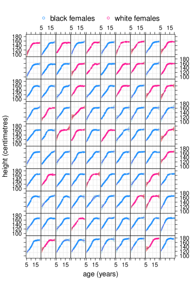
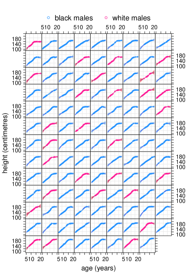
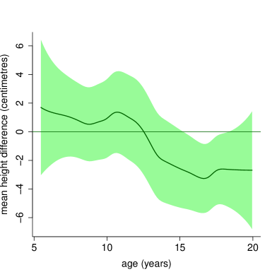
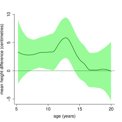
Figure 2: Top panels: fitted group-specific curves for 100 female subjects (left) and 116 male subjects (right) from the data on adolescent somatic growth (Pratt et al. 1989). The shading corresponds to approximate pointwise 99% credible intervals. Bottom panels: similar to the top panels but for the estimated contrast curve. The shaded regions correspond to approximate pointwise 95% credible intervals.

3 Three-Level Models

The three-level version of group-specific curve models corresponds to curve-type data having two nested groupings. For example, the data in each panel of Figure 1 are first grouped according to slice, which is the level 2 group, and the slices are grouped according to tumor which is the level 3 group. We denote predictor/response pairs as $(x_{ijk},y_{ijk})$ where $x_{ijk}$ is the $k$th value of the predictor variable in the $i$th level 3 group and $(i,j)$th level 2 group and $y_{ijk}$ is the corresponding value of the response variable. We let $m$ denote the number of level 3 groups, $n_{i}$ denote that number of level 2 groups in the $i$th level 3 group and $o_{ij}$ denote the the number of units within the $(i,j)$th level 2 group. The Figure 1 data, which happen to be balanced, are such that

$$m = \mbox{number of tumors}=10,$$

$$n_{i} = \mbox{number of slices for the $i$th tumor}=5$$

$$\mbox{and}\ \ o_{ij} = \mbox{number of predictor/response pairs for the $i$th tumor and $j$th slice}=128.$$

The Gaussian response three-level group specific curve model for such data is

$$\begin{array}[]{l}y_{ijk}=f(x_{ijk})+g_{i}(x_{ijk})+h_{ij}(x_{ijk})+\varepsilon_{ijk},\quad\varepsilon_{ijk}\stackrel{{\scriptstyle{\tiny\mbox{ind.}}}}{{\sim}}N(0,\sigma_{\varepsilon}^{2}),\\[8.61108pt] \quad 1\leq i\leq m,\ 1\leq j\leq n_{i},\ 1\leq k\leq o_{ij},\end{array}$$ (17)

where the smooth function $f$ is the global mean function, the $g_{i}$ functions, $1\leq i\leq m$, allow for group-specific deviations according to membership of the $i$th level 3 group and the $h_{ij}$, $1\leq i\leq m$ and $1\leq j\leq n_{i}$ allow for an additional level of group-specific deviations according to membership of the $j$th level 2 group within the $i$th level 3 group. The mixed model-based penalized spline models for these functions are

$$f(x) = \beta_{0}+\beta_{1}\,x+\sum_{k=1}^{K_{\mbox{\rm\tiny gbl}}}\,u_{\mbox{\rm\tiny gbl,$k$}}\,z_{\mbox{\rm\tiny gbl,$k$}}(x),\quad u_{\mbox{\rm\tiny gbl,$k$}}\stackrel{{\scriptstyle{\tiny\mbox{ind.}}}}{{\sim}}N(0,\sigma_{\mbox{\rm\tiny gbl}}^{2}),$$

$$g_{i}(x) = u_{\mbox{\rm\tiny lin,$i0$}}^{g}+u_{\mbox{\rm\tiny lin,$i1$}}^{g}\,x+\sum_{k=1}^{K_{\mbox{\rm\tiny grp}}^{g}}\,u_{\mbox{\rm\tiny grp,$ik$}}^{g}\,z_{\mbox{\rm\tiny grp,k}}^{g}(x),\ \left[\begin{array}[]{c}u_{\mbox{\rm\tiny lin,$i0$}}^{g}\\[4.30554pt] u_{\mbox{\rm\tiny lin,$i1$}}^{g}\end{array}\right]\stackrel{{\scriptstyle{\tiny\mbox{ind.}}}}{{\sim}}N(\boldsymbol{0},\boldsymbol{\Sigma}_{\mbox{\rm\tiny$g$}}),\ u_{\mbox{\rm\tiny grp,$ik$}}^{g}\stackrel{{\scriptstyle{\tiny\mbox{ind.}}}}{{\sim}}N\big{(}0,\sigma_{\mbox{\rm\tiny grp,$g$}}^{2}\big{)}$$

and

$$h_{ij}(x) = u_{\mbox{\rm\tiny lin,$ij0$}}^{h}+u_{\mbox{\rm\tiny lin,$ij1$}}^{h}\,x+\sum_{k=1}^{K_{\mbox{\rm\tiny grp}}^{h}}\,u_{\mbox{\rm\tiny grp,$ijk$}}^{h}\,z_{\mbox{\rm\tiny grp,k}}^{h}(x),\ \left[\begin{array}[]{c}u_{\mbox{\rm\tiny lin,$ij0$}}^{h}\\[4.30554pt] u_{\mbox{\rm\tiny lin,$ij1$}}^{h}\end{array}\right]\stackrel{{\scriptstyle{\tiny\mbox{ind.}}}}{{\sim}}N(\boldsymbol{0},\boldsymbol{\Sigma}_{\mbox{\rm\tiny$h$}}),\ u_{\mbox{\rm\tiny grp,$ijk$}}^{h}\stackrel{{\scriptstyle{\tiny\mbox{ind.}}}}{{\sim}}N\big{(}0,\sigma_{\mbox{\rm\tiny grp,$h$}}^{2}\big{)},$$

with all random effect distributions independent of each other. For this three-level case we have three bases:

$$\{z_{\mbox{\rm\tiny gbl,$k$}}(\cdot):1\leq k\leq K_{\mbox{\rm\tiny gbl}}\},\quad\{z_{\mbox{\rm\tiny grp,k}}^{g}(\cdot):1\leq k\leq K_{\mbox{\rm\tiny grp}}^{g}\}\quad\mbox{and}\quad\{z_{\mbox{\rm\tiny grp,k}}^{h}(\cdot):1\leq k\leq K_{\mbox{\rm\tiny grp}}^{h}\}.$$

The variance and covariance matrix parameters are analogous to the two-level model. For example, $\boldsymbol{\Sigma}_{\mbox{\rm\tiny$g$}}$ and $\boldsymbol{\Sigma}_{\mbox{\rm\tiny$h$}}$ are both unstructured $2\times 2$ matrices corresponding to the linear components of the $g_{i}$ and $h_{ij}$ respectively.

The following notation is useful for setting up the required design matrices: if $\boldsymbol{M}_{1},\ldots,\boldsymbol{M}_{d}$ is a set of matrices each having the same number of columns then

$$\mathop{\mbox{\rm stack}}_{1\leq i\leq d}(\boldsymbol{M}_{i})\equiv\left[\begin{array}[]{c}\boldsymbol{M}_{1}\\ \vdots\\ \boldsymbol{M}_{d}\end{array}\right].$$

We then define, for $1\leq i\leq m$ and $1\leq j\leq n_{i}$,

$$\boldsymbol{x}_{i}\equiv\mathop{\mbox{\rm stack}}_{1\leq j\leq n_{i}}\big{(}\boldsymbol{x}_{ij}\big{)}\quad\mbox{and}\quad\boldsymbol{x}_{ij}\equiv\mathop{\mbox{\rm stack}}_{1\leq k\leq\,o_{ij}}\big{(}x_{ijk}\big{)}.$$

3.1 Best Linear Unbiased Prediction

Model (17) is expressible as a Gaussian response linear mixed model as follows:

$$\boldsymbol{y}|\boldsymbol{u}\sim N(\boldsymbol{X}\boldsymbol{\beta}+\boldsymbol{Z}\,\boldsymbol{u},\sigma_{\varepsilon}^{2}\,\boldsymbol{I}),\quad\boldsymbol{u}\sim N(\boldsymbol{0},\boldsymbol{G}),$$ (20)

where the design matrices are

$$\boldsymbol{X}=\mathop{\mbox{\rm stack}}_{1\leq i\leq m}\big{(}\boldsymbol{X}_{i}\big{)}\quad\mbox{with}\quad\boldsymbol{X}_{i}=\mathop{\mbox{\rm stack}}_{1\leq j\leq n_{i}}\big{(}\boldsymbol{X}_{ij}\big{)}\quad\mbox{and}\quad\boldsymbol{X}_{ij}\equiv[\boldsymbol{1}\ \boldsymbol{x}_{ij}]$$

and

$$\boldsymbol{Z}\equiv\Big{[}\boldsymbol{Z}_{\mbox{\rm\tiny gbl}}\,\mathop{\mbox{\rm blockdiag}}_{1\leq i\leq m}\Big{[}\mathop{\mbox{\rm stack}}_{1\leq j\leq n_{i}}([\boldsymbol{X}_{ij}\ \boldsymbol{Z}^{\mbox{\rm\tiny$g$}}_{\mbox{\rm\tiny grp,$ij$}}])\,\mathop{\mbox{\rm blockdiag}}_{1\leq j\leq n_{i}}([\boldsymbol{X}_{ij}\ \boldsymbol{Z}^{\mbox{\rm\tiny$h$}}_{\mbox{\rm\tiny grp,$ij$}}])\Big{]}\Big{]}.$$

where

$$\boldsymbol{Z}_{\mbox{\rm\tiny gbl}}\equiv\mathop{\mbox{\rm stack}}_{1\leq i\leq m}\big{(}\mathop{\mbox{\rm stack}}_{1\leq j\leq n_{i}}(\boldsymbol{Z}_{\mbox{\rm\tiny gbl,$ij$}})\big{)}$$

and the matrices $\boldsymbol{Z}_{\mbox{\rm\tiny gbl,$ij$}}$, $\boldsymbol{Z}^{\mbox{\rm\tiny$g$}}_{\mbox{\rm\tiny grp,$ij$}}$ and $\boldsymbol{Z}^{\mbox{\rm\tiny$h$}}_{\mbox{\rm\tiny grp,$ij$}}$, $1\leq i\leq m$, $1\leq j\leq n_{i}$, contain, respectively, spline basis functions for the global mean function $f$, the $i$th level one group deviation functions $g_{i}$ and $(i,j)$th level two group deviation functions $h_{ij}$. Specifically,

$$\boldsymbol{Z}_{\mbox{\rm\tiny gbl,$ij$}} \equiv [\begin{array}[]{ccc}z_{\mbox{\rm\tiny gbl,$1$}}(\boldsymbol{x}_{ij})&\cdots&z_{\mbox{\rm\tiny gbl,$K_{\mbox{\rm\tiny gbl}}$}}(\boldsymbol{x}_{ij})\end{array}],\quad\boldsymbol{Z}^{\mbox{\rm\tiny$g$}}_{\mbox{\rm\tiny grp,$ij$}}=[z_{\mbox{\rm\tiny grp,$1$}}^{\mbox{\rm\tiny$g$}}(\boldsymbol{x}_{ij})\cdots z_{\mbox{\rm\tiny grp,$K_{\mbox{\rm\tiny grp}}^{\mbox{\rm\tiny$g$}}$}}^{\mbox{\rm\tiny$g$}}(\boldsymbol{x}_{ij})]$$

$$\mbox{and}\ \boldsymbol{Z}^{\mbox{\rm\tiny$h$}}_{\mbox{\rm\tiny grp,$ij$}} \equiv [z_{\mbox{\rm\tiny grp,$1$}}^{\mbox{\rm\tiny$h$}}(\boldsymbol{x}_{ij})\cdots z_{\mbox{\rm\tiny grp,$K_{\mbox{\rm\tiny grp}}^{\mbox{\rm\tiny$h$}}$}}^{\mbox{\rm\tiny$h$}}(\boldsymbol{x}_{ij})]\quad\mbox{for $1\leq i\leq m$ and $1\leq j\leq n_{i}$.}$$

The fixed and random effects vectors are

$$\boldsymbol{\beta}\equiv\left[\begin{array}[]{c}\beta_{0}\\[4.30554pt] \beta_{1}\end{array}\right]\quad\mbox{and}\quad\boldsymbol{u}\equiv\left[\begin{array}[]{c}\boldsymbol{u}_{\mbox{\rm\tiny gbl}}\\[4.30554pt] {\displaystyle\mathop{\mbox{\rm stack}}_{1\leq i\leq m}}\left(\left[\begin{array}[]{c}\left[\begin{array}[]{c}\boldsymbol{u}^{\mbox{\rm\tiny$g$}}_{\mbox{\rm\tiny lin,$i$}}\\ \boldsymbol{u}^{\mbox{\rm\tiny$g$}}_{\mbox{\rm\tiny grp,$i$}}\end{array}\right]\\[8.61108pt] \left[\begin{array}[]{c}\boldsymbol{u}^{\mbox{\rm\tiny$h$}}_{\mbox{\rm\tiny lin,$i$1}}\\ \boldsymbol{u}^{\mbox{\rm\tiny$h$}}_{\mbox{\rm\tiny grp,$i1$}}\end{array}\right]\\[8.61108pt] \vdots\\[8.61108pt] \left[\begin{array}[]{c}\boldsymbol{u}^{\mbox{\rm\tiny$h$}}_{\mbox{\rm\tiny lin,$in_{i}$}}\\ \boldsymbol{u}^{\mbox{\rm\tiny$h$}}_{\mbox{\rm\tiny grp,$in_{i}$}}\end{array}\right]\end{array}\right]\right)\end{array}\right]\quad\mbox{where}\quad\boldsymbol{u}^{\mbox{\rm\tiny$g$}}_{\mbox{\rm\tiny lin,$i$}}\equiv\left[\begin{array}[]{c}u_{\mbox{\rm\tiny lin,$i0$}}^{g}\\[4.30554pt] u_{\mbox{\rm\tiny lin,$i1$}}^{g}\end{array}\right]$$

with $\boldsymbol{u}^{\mbox{\rm\tiny$g$}}_{\mbox{\rm\tiny grp,$i$}}$, $\boldsymbol{u}^{\mbox{\rm\tiny$h$}}_{\mbox{\rm\tiny lin,$ij$}}$ and $\boldsymbol{u}^{\mbox{\rm\tiny$h$}}_{\mbox{\rm\tiny grp,$ij$}}$ defined similarly and the covariance matrix of $\boldsymbol{u}$ is

$$\begin{array}[]{c}\boldsymbol{G}=\mbox{\rm Cov}(\boldsymbol{u})=\left[\begin{array}[]{cc}\sigma_{\mbox{\rm\tiny gbl}}^{2}\boldsymbol{I}&\boldsymbol{O}\\[4.30554pt] \boldsymbol{O}&\displaystyle{\mathop{\mbox{\rm blockdiag}}_{1\leq i\leq m}}\left[\begin{array}[]{ccc}\boldsymbol{\Sigma}_{\mbox{\rm\tiny$g$}}&\boldsymbol{O}&\boldsymbol{O}\\ \boldsymbol{O}&\sigma_{\mbox{\rm\tiny grp,$g$}}^{2}\boldsymbol{I}&\boldsymbol{O}\\ \boldsymbol{O}&\boldsymbol{O}&\boldsymbol{I}_{n_{i}}\otimes\left[\begin{array}[]{cc}\boldsymbol{\Sigma}_{\mbox{\rm\tiny$h$}}&\boldsymbol{O}\\ \boldsymbol{O}&\sigma_{\mbox{\rm\tiny grp,$h$}}^{2}\boldsymbol{I}\end{array}\right]\end{array}\right]\end{array}\right].\end{array}$$ (22)

We define matrices in a similar way to what is given in (6). The best linear unbiased predictor of $[\boldsymbol{\beta}\ \boldsymbol{u}]$ and corresponding covariance matrix are as shown in (7), but, with entries as described in this section. This covariance matrix grows quadratically in both $m$ and the $n_{i}$s, and so, storage becomes impractical for large numbers of level 2 and level 3 groups. However, only certain sub-blocks are required for the addition of pointwise confidence intervals to curve estimates. In particular, we only require the non-zero sub-blocks of the general three-level sparse matrix given in Section 3 of Nolan & Wand (2018) that correspond to $(\boldsymbol{C}^{T}\boldsymbol{R}_{\mbox{{\bf BLUP}}}^{-1}\boldsymbol{C}+\boldsymbol{D}_{\mbox{{\bf BLUP}}})^{-1}$. In the case of the three-level Gaussian response linear model, Nolan & Wand’s

$$\begin{array}[]{l}\boldsymbol{A}_{11}\mbox{ sub-block corresponds to a }(2+K_{\mbox{\rm\tiny gbl}})\times(2+K_{\mbox{\rm\tiny gbl}})\mbox{ matrix }\mbox{\rm Cov}\left(\left[\begin{array}[]{c}{\widehat{\boldsymbol{\beta}}}\\ {\widehat{\boldsymbol{u}}}_{\mbox{\rm\tiny gbl}}-\boldsymbol{u}_{\mbox{\rm\tiny gbl}}\end{array}\right]\right);\\[8.61108pt] \boldsymbol{A}_{22,i}\mbox{ sub-block corresponds to a }(2+K_{\mbox{\rm\tiny grp}}^{\mbox{\rm\tiny$g$}})\times(2+K_{\mbox{\rm\tiny grp}}^{\mbox{\rm\tiny$g$}})\mbox{ matrix }\mbox{\rm Cov}\left(\left[\begin{array}[]{c}{\widehat{\boldsymbol{u}}}^{\mbox{\rm\tiny$g$}}_{\mbox{\rm\tiny lin,$i$}}-\boldsymbol{u}^{\mbox{\rm\tiny$g$}}_{\mbox{\rm\tiny lin,$i$}}\\[4.30554pt] {\widehat{\boldsymbol{u}}}^{\mbox{\rm\tiny$g$}}_{\mbox{\rm\tiny grp,$i$}}-\boldsymbol{u}^{\mbox{\rm\tiny$g$}}_{\mbox{\rm\tiny grp,$i$}}\end{array}\right]\right);\\[4.30554pt] \boldsymbol{A}_{12,i}\mbox{ sub-block corresponds to a }(2+K_{\mbox{\rm\tiny gbl}})\times(2+K_{\mbox{\rm\tiny grp}}^{\mbox{\rm\tiny$g$}})\mbox{ matrix }\\[4.30554pt] \qquad\qquad\qquad E\left\{\left[\begin{array}[]{c}{\widehat{\boldsymbol{\beta}}}\\ {\widehat{\boldsymbol{u}}}_{\mbox{\rm\tiny gbl}}-\boldsymbol{u}_{\mbox{\rm\tiny gbl}}\end{array}\right]\left[\begin{array}[]{c}{\widehat{\boldsymbol{u}}}^{\mbox{\rm\tiny$g$}}_{\mbox{\rm\tiny lin,$i$}}-\boldsymbol{u}^{\mbox{\rm\tiny$g$}}_{\mbox{\rm\tiny lin,$i$}}\\[4.30554pt] {\widehat{\boldsymbol{u}}}^{\mbox{\rm\tiny$g$}}_{\mbox{\rm\tiny grp,$i$}}-\boldsymbol{u}^{\mbox{\rm\tiny$g$}}_{\mbox{\rm\tiny grp,$i$}}\end{array}\right]^{T}\right\},\ 1\leq i\leq m;\\[4.30554pt] \boldsymbol{A}_{22,ij}\mbox{ sub-block corresponds to a }(2+K_{\mbox{\rm\tiny grp}}^{\mbox{\rm\tiny$h$}})\times(2+K_{\mbox{\rm\tiny grp}}^{\mbox{\rm\tiny$h$}})\mbox{ matrix }\mbox{\rm Cov}\left(\left[\begin{array}[]{c}{\widehat{\boldsymbol{u}}}^{\mbox{\rm\tiny$h$}}_{\mbox{\rm\tiny lin,$ij$}}-\boldsymbol{u}^{\mbox{\rm\tiny$h$}}_{\mbox{\rm\tiny lin,$ij$}}\\[4.30554pt] {\widehat{\boldsymbol{u}}}^{\mbox{\rm\tiny$h$}}_{\mbox{\rm\tiny grp,$ij$}}-\boldsymbol{u}^{\mbox{\rm\tiny$h$}}_{\mbox{\rm\tiny grp,$ij$}}\end{array}\right]\right);\\[4.30554pt] \boldsymbol{A}_{12,ij}\mbox{ sub-block corresponds to a }(2+K_{\mbox{\rm\tiny gbl}})\times(2+K_{\mbox{\rm\tiny grp}}^{\mbox{\rm\tiny$h$}})\mbox{ matrix }\\[4.30554pt] \qquad\qquad\qquad E\left\{\left[\begin{array}[]{c}{\widehat{\boldsymbol{\beta}}}\\ {\widehat{\boldsymbol{u}}}_{\mbox{\rm\tiny gbl}}-\boldsymbol{u}_{\mbox{\rm\tiny gbl}}\end{array}\right]\left[\begin{array}[]{c}{\widehat{\boldsymbol{u}}}^{\mbox{\rm\tiny$h$}}_{\mbox{\rm\tiny lin,$ij$}}-\boldsymbol{u}^{\mbox{\rm\tiny$h$}}_{\mbox{\rm\tiny lin,$ij$}}\\[4.30554pt] {\widehat{\boldsymbol{u}}}^{\mbox{\rm\tiny$h$}}_{\mbox{\rm\tiny grp,$ij$}}-\boldsymbol{u}^{\mbox{\rm\tiny$h$}}_{\mbox{\rm\tiny grp,$ij$}}\end{array}\right]^{T}\right\};\\[4.30554pt] \boldsymbol{A}_{12,\,i,\,j}\mbox{ sub-block corresponds to a }(2+K_{\mbox{\rm\tiny grp}}^{\mbox{\rm\tiny$g$}})\times(2+K_{\mbox{\rm\tiny grp}}^{\mbox{\rm\tiny$h$}})\mbox{ matrix }\\[4.30554pt] \qquad\qquad\qquad E\left\{\left[\begin{array}[]{c}{\widehat{\boldsymbol{u}}}^{\mbox{\rm\tiny$g$}}_{\mbox{\rm\tiny lin,$i$}}-\boldsymbol{u}^{\mbox{\rm\tiny$g$}}_{\mbox{\rm\tiny lin,$i$}}\\[4.30554pt] {\widehat{\boldsymbol{u}}}^{\mbox{\rm\tiny$g$}}_{\mbox{\rm\tiny grp,$i$}}-\boldsymbol{u}^{\mbox{\rm\tiny$g$}}_{\mbox{\rm\tiny grp,$i$}}\end{array}\right]\left[\begin{array}[]{c}{\widehat{\boldsymbol{u}}}^{\mbox{\rm\tiny$h$}}_{\mbox{\rm\tiny lin,$ij$}}-\boldsymbol{u}^{\mbox{\rm\tiny$h$}}_{\mbox{\rm\tiny lin,$ij$}}\\[4.30554pt] {\widehat{\boldsymbol{u}}}^{\mbox{\rm\tiny$h$}}_{\mbox{\rm\tiny grp,$ij$}}-\boldsymbol{u}^{\mbox{\rm\tiny$h$}}_{\mbox{\rm\tiny grp,$ij$}}\end{array}\right]^{T}\right\},\ 1\leq i\leq m,\ 1\leq j\leq n_{i}.\end{array}$$

As described in Nolan, Menictas & Wand (2019), the SolveThreeLevelSparseLeastSquares algorithm arises in the special case where $\boldsymbol{x}$ is the minimizer of the least squares problem given in equation (9), where $\boldsymbol{B}$ has the three-level sparse form and $\boldsymbol{b}$ is partitioned according to that shown in equation (7) of Nolan & Wand (2018). This algorithm can be used for fitting three-level group-specific curve models by making use of Result 3.

Result 3.

Computation of $[{\widehat{\boldsymbol{\beta}}}^{T}\ \ {\widehat{\boldsymbol{u}}}^{T}]^{T}$ and each of the sub-blocks of $\mbox{\rm Cov}([{\widehat{\boldsymbol{\beta}}}^{T}\ \ ({\widehat{\boldsymbol{u}}}-\boldsymbol{u})^{T}]^{T})$ listed in (8) are expressible as the three-level sparse matrix least squares form:

$$\left\|\boldsymbol{b}-\boldsymbol{B}\left[\begin{array}[]{c}\boldsymbol{\beta}\\ \boldsymbol{u}\end{array}\right]\right\|^{2}$$

where the non-zero sub-blocks $\boldsymbol{B}$ and $\boldsymbol{b}$, according to the notation in Section 3.1 of Nolan & Wand (2018), are for $1\leq i\leq m$ and $1\leq j\leq n_{i}$:

$$\boldsymbol{b}_{ij}\equiv\left[\begin{array}[]{c}\sigma_{\varepsilon}^{-1}\boldsymbol{y}_{ij}\\[4.30554pt] \boldsymbol{0}\\[4.30554pt] \boldsymbol{0}\\[4.30554pt] \boldsymbol{0}\\[4.30554pt] \boldsymbol{0}\\[4.30554pt] \boldsymbol{0}\\[4.30554pt] \end{array}\right],\qquad\boldsymbol{B}_{ij}\equiv\left[\begin{array}[]{cc}\sigma_{\varepsilon}^{-1}\boldsymbol{X}_{ij}&\sigma_{\varepsilon}^{-1}\boldsymbol{Z}_{\mbox{\rm\tiny gbl,$ij$}}\\[4.30554pt] \boldsymbol{O}&\left(\sum_{i=1}^{m}n_{i}\right)^{-1/2}\sigma_{\mbox{\rm\tiny gbl}}^{-1}\boldsymbol{I}_{K_{\mbox{\rm\tiny gbl}}}\\[4.30554pt] \boldsymbol{O}&\boldsymbol{O}\\[4.30554pt] \boldsymbol{O}&\boldsymbol{O}\\[4.30554pt] \boldsymbol{O}&\boldsymbol{O}\\[4.30554pt] \boldsymbol{O}&\boldsymbol{O}\\[4.30554pt] \end{array}\right],$$

$$\overset{\ \mbox{{$\bullet$}}}{\boldsymbol{B}}_{ij}\equiv\left[\begin{array}[]{cc}\sigma_{\varepsilon}^{-1}\boldsymbol{X}_{ij}&\sigma_{\varepsilon}^{-1}\boldsymbol{Z}^{\mbox{\rm\tiny$g$}}_{\mbox{\rm\tiny grp,$ij$}}\\[4.30554pt] \boldsymbol{O}&\boldsymbol{O}\\[4.30554pt] n_{i}^{-1/2}\boldsymbol{\Sigma}_{\mbox{\rm\tiny$g$}}^{-1/2}&\boldsymbol{O}\\[4.30554pt] \boldsymbol{O}&n_{i}^{-1/2}\sigma_{\mbox{\rm\tiny grp,$g$}}^{-1}\boldsymbol{I}_{K_{\mbox{\rm\tiny grp}}^{\mbox{\rm\tiny$g$}}}\\[4.30554pt] \boldsymbol{O}&\boldsymbol{O}\\[4.30554pt] \boldsymbol{O}&\boldsymbol{O}\\[4.30554pt] \end{array}\right]\quad and\quad\overset{\mbox{{$\bullet$}}\mbox{{$\bullet$}}}{\boldsymbol{B}}_{ij}\equiv\left[\begin{array}[]{cc}\sigma_{\varepsilon}^{-1}\boldsymbol{X}_{ij}&\sigma_{\varepsilon}^{-1}\boldsymbol{Z}^{\mbox{\rm\tiny$h$}}_{\mbox{\rm\tiny grp,$ij$}}\\[4.30554pt] \boldsymbol{O}&\boldsymbol{O}\\[4.30554pt] \boldsymbol{O}&\boldsymbol{O}\\[4.30554pt] \boldsymbol{O}&\boldsymbol{O}\\[4.30554pt] \boldsymbol{\Sigma}_{\mbox{\rm\tiny$h$}}^{-1/2}&\boldsymbol{O}\\[4.30554pt] \boldsymbol{O}&\sigma_{\mbox{\rm\tiny grp,$h$}}^{-1}\boldsymbol{I}_{K_{\mbox{\rm\tiny grp}}^{\mbox{\rm\tiny$h$}}}\end{array}\right]$$

with each of these matrices having ${\tilde{o}}_{ij}=o_{ij}+K_{\mbox{\rm\tiny gbl}}+2+K_{\mbox{\rm\tiny grp}}^{\mbox{\rm\tiny$g$}}+2+K_{\mbox{\rm\tiny grp}}^{\mbox{\rm\tiny$h$}}$ rows and with $\boldsymbol{B}_{i}$ having $p=2+K_{\mbox{\rm\tiny gbl}}$ columns, $\overset{\ \mbox{{$\bullet$}}}{\boldsymbol{B}}_{i}$ having $q_{1}=2+K_{\mbox{\rm\tiny grp}}^{\mbox{\rm\tiny$g$}}$ columns and $\overset{\mbox{{$\bullet$}}\mbox{{$\bullet$}}}{\boldsymbol{B}}_{ij}$ having $q_{2}=2+K_{\mbox{\rm\tiny grp}}^{\mbox{\rm\tiny$h$}}$ columns. The solutions are

$$\left[\begin{array}[]{c}{\widehat{\boldsymbol{\beta}}}\\ {\widehat{\boldsymbol{u}}}_{\mbox{\rm\tiny gbl}}\end{array}\right]=\boldsymbol{x}_{1},\quad\mbox{\rm Cov}\left(\left[\begin{array}[]{c}{\widehat{\boldsymbol{\beta}}}\\ {\widehat{\boldsymbol{u}}}_{\mbox{\rm\tiny gbl}}-\boldsymbol{u}_{\mbox{\rm\tiny gbl}}\end{array}\right]\right)=\boldsymbol{A}^{11},$$

$$\left[\begin{array}[]{c}{\widehat{\boldsymbol{u}}}^{\mbox{\rm\tiny$g$}}_{\mbox{\rm\tiny lin,$i$}}\\[4.30554pt] {\widehat{\boldsymbol{u}}}^{\mbox{\rm\tiny$g$}}_{\mbox{\rm\tiny grp,$i$}}\end{array}\right]=\boldsymbol{x}_{2,i},\quad E\left\{\left[\begin{array}[]{c}{\widehat{\boldsymbol{\beta}}}\\ {\widehat{\boldsymbol{u}}}_{\mbox{\rm\tiny gbl}}-\boldsymbol{u}_{\mbox{\rm\tiny gbl}}\end{array}\right]\left[\begin{array}[]{c}{\widehat{\boldsymbol{u}}}^{\mbox{\rm\tiny$g$}}_{\mbox{\rm\tiny lin,$i$}}-\boldsymbol{u}^{\mbox{\rm\tiny$g$}}_{\mbox{\rm\tiny lin,$i$}}\\[4.30554pt] {\widehat{\boldsymbol{u}}}^{\mbox{\rm\tiny$g$}}_{\mbox{\rm\tiny grp,$i$}}-\boldsymbol{u}^{\mbox{\rm\tiny$g$}}_{\mbox{\rm\tiny grp,$i$}}\end{array}\right]^{T}\right\}=\boldsymbol{A}^{12,i},$$

$$\mbox{\rm Cov}\left(\left[\begin{array}[]{c}{\widehat{\boldsymbol{u}}}^{\mbox{\rm\tiny$g$}}_{\mbox{\rm\tiny lin,$i$}}-\boldsymbol{u}^{\mbox{\rm\tiny$g$}}_{\mbox{\rm\tiny lin,$i$}}\\[4.30554pt] {\widehat{\boldsymbol{u}}}^{\mbox{\rm\tiny$g$}}_{\mbox{\rm\tiny grp,$i$}}-\boldsymbol{u}^{\mbox{\rm\tiny$g$}}_{\mbox{\rm\tiny grp,$i$}}\end{array}\right]\right)=\boldsymbol{A}^{22,i},\ \ 1\leq i\leq m,$$

$$\left[\begin{array}[]{c}{\widehat{\boldsymbol{u}}}^{\mbox{\rm\tiny$h$}}_{\mbox{\rm\tiny lin,$ij$}}\\[4.30554pt] {\widehat{\boldsymbol{u}}}^{\mbox{\rm\tiny$h$}}_{\mbox{\rm\tiny grp,$ij$}}\end{array}\right]=\boldsymbol{x}_{2,ij},\quad E\left\{\left[\begin{array}[]{c}{\widehat{\boldsymbol{\beta}}}\\ {\widehat{\boldsymbol{u}}}_{\mbox{\rm\tiny gbl}}-\boldsymbol{u}_{\mbox{\rm\tiny gbl}}\end{array}\right]\left[\begin{array}[]{c}{\widehat{\boldsymbol{u}}}^{\mbox{\rm\tiny$h$}}_{\mbox{\rm\tiny lin,$ij$}}-\boldsymbol{u}^{\mbox{\rm\tiny$h$}}_{\mbox{\rm\tiny lin,$ij$}}\\[4.30554pt] {\widehat{\boldsymbol{u}}}^{\mbox{\rm\tiny$h$}}_{\mbox{\rm\tiny grp,$ij$}}-\boldsymbol{u}^{\mbox{\rm\tiny$h$}}_{\mbox{\rm\tiny grp,$ij$}}\end{array}\right]^{T}\right\}=\boldsymbol{A}^{12,ij},$$

$$E\left\{\left[\begin{array}[]{c}{\widehat{\boldsymbol{u}}}^{\mbox{\rm\tiny$g$}}_{\mbox{\rm\tiny lin,$i$}}-\boldsymbol{u}^{\mbox{\rm\tiny$g$}}_{\mbox{\rm\tiny lin,$i$}}\\[4.30554pt] {\widehat{\boldsymbol{u}}}^{\mbox{\rm\tiny$g$}}_{\mbox{\rm\tiny grp,$i$}}-\boldsymbol{u}^{\mbox{\rm\tiny$g$}}_{\mbox{\rm\tiny grp,$i$}}\end{array}\right]\left[\begin{array}[]{c}{\widehat{\boldsymbol{u}}}^{\mbox{\rm\tiny$h$}}_{\mbox{\rm\tiny lin,$ij$}}-\boldsymbol{u}^{\mbox{\rm\tiny$h$}}_{\mbox{\rm\tiny lin,$ij$}}\\[4.30554pt] {\widehat{\boldsymbol{u}}}^{\mbox{\rm\tiny$h$}}_{\mbox{\rm\tiny grp,$ij$}}-\boldsymbol{u}^{\mbox{\rm\tiny$h$}}_{\mbox{\rm\tiny grp,$ij$}}\end{array}\right]^{T}\right\}=\boldsymbol{A}^{12,\,i,\,j}$$

and

$$\mbox{\rm Cov}\left(\left[\begin{array}[]{c}{\widehat{\boldsymbol{u}}}^{\mbox{\rm\tiny$h$}}_{\mbox{\rm\tiny lin,$ij$}}-\boldsymbol{u}^{\mbox{\rm\tiny$h$}}_{\mbox{\rm\tiny lin,$ij$}}\\[4.30554pt] {\widehat{\boldsymbol{u}}}^{\mbox{\rm\tiny$h$}}_{\mbox{\rm\tiny grp,$ij$}}-\boldsymbol{u}^{\mbox{\rm\tiny$h$}}_{\mbox{\rm\tiny grp,$ij$}}\end{array}\right]\right)=\boldsymbol{A}^{22,ij},\quad 1\leq i\leq m,\ 1\leq j\leq n_{i}.$$

• Inputs: $\boldsymbol{y}_{ij}(o_{ij}\times 1),\ \boldsymbol{X}_{ij}(o_{ij}\times 2),\ \boldsymbol{Z}_{\mbox{\rm\tiny gbl,$ij$}}(o_{ij}\times K_{\mbox{\rm\tiny gbl}}),\ \boldsymbol{Z}^{\mbox{\rm\tiny$g$}}_{\mbox{\rm\tiny grp,$ij$}}(o_{ij}\times K_{\mbox{\rm\tiny grp}}^{\mbox{\rm\tiny$g$}}),$

• $\boldsymbol{Z}^{\mbox{\rm\tiny$h$}}_{\mbox{\rm\tiny grp,$ij$}}(o_{ij}\times K_{\mbox{\rm\tiny grp}}^{\mbox{\rm\tiny$h$}}),1\leq i\leq m,\ 1\leq j\leq n_{i}$; $\quad\sigma_{\varepsilon}^{2},\sigma_{\mbox{\rm\tiny gbl}}^{2},\sigma_{\mbox{\rm\tiny grp,$g$}}^{2},\sigma_{\mbox{\rm\tiny grp,$h$}}^{2}>0$,

• $\boldsymbol{\Sigma}_{\mbox{\rm\tiny$g$}}(2\times 2),\ \boldsymbol{\Sigma}_{\mbox{\rm\tiny$h$}}(2\times 2),\mbox{symmetric and positive definite.}$

• For $i=1,\ldots,m$:

  • For $j=1,\ldots,n_{i}$:

    • $\begin{array}[]{l}\boldsymbol{b}_{ij}\longleftarrow\left[\begin{array}[]{c}\sigma_{\varepsilon}^{-1}\boldsymbol{y}_{ij}\\[3.87498pt] \boldsymbol{0}\\[3.87498pt] \boldsymbol{0}\\[3.87498pt] \boldsymbol{0}\\[3.87498pt] \boldsymbol{0}\\[3.87498pt] \boldsymbol{0}\\[3.87498pt] \end{array}\right],\ \boldsymbol{B}_{ij}\longleftarrow\left[\begin{array}[]{cc}\sigma_{\varepsilon}^{-1}\boldsymbol{X}_{ij}&\sigma_{\varepsilon}^{-1}\boldsymbol{Z}_{\mbox{\rm\tiny gbl,$ij$}}\\[3.87498pt] \boldsymbol{O}&\left(\sum_{i=1}^{m}n_{i}\right)^{-1/2}\sigma_{\mbox{\rm\tiny gbl}}^{-1}\boldsymbol{I}_{K_{\mbox{\rm\tiny gbl}}}\\[3.87498pt] \boldsymbol{O}&\boldsymbol{O}\\[3.87498pt] \boldsymbol{O}&\boldsymbol{O}\\[3.87498pt] \boldsymbol{O}&\boldsymbol{O}\\[3.87498pt] \boldsymbol{O}&\boldsymbol{O}\\[3.87498pt] \end{array}\right]\end{array}$

    • $\begin{array}[]{l}\overset{\ \mbox{{$\bullet$}}}{\boldsymbol{B}}_{ij}\longleftarrow\left[\begin{array}[]{cc}\sigma_{\varepsilon}^{-1}\boldsymbol{X}_{ij}&\sigma_{\varepsilon}^{-1}\boldsymbol{Z}^{\mbox{\rm\tiny$g$}}_{\mbox{\rm\tiny grp,$ij$}}\\[3.87498pt] \boldsymbol{O}&\boldsymbol{O}\\[3.87498pt] n_{i}^{-1/2}\boldsymbol{\Sigma}_{\mbox{\rm\tiny$g$}}^{-1/2}&\boldsymbol{O}\\[3.87498pt] \boldsymbol{O}&n_{i}^{-1/2}\sigma_{\mbox{\rm\tiny grp,$g$}}^{-1}\boldsymbol{I}_{K_{\mbox{\rm\tiny grp}}^{\mbox{\rm\tiny$g$}}}\\[3.87498pt] \boldsymbol{O}&\boldsymbol{O}\\[3.87498pt] \boldsymbol{O}&\boldsymbol{O}\\[3.87498pt] \end{array}\right],\ \overset{\mbox{{$\bullet$}}\mbox{{$\bullet$}}}{\boldsymbol{B}}_{ij}\longleftarrow\left[\begin{array}[]{cc}\sigma_{\varepsilon}^{-1}\boldsymbol{X}_{ij}&\sigma_{\varepsilon}^{-1}\boldsymbol{Z}^{\mbox{\rm\tiny$h$}}_{\mbox{\rm\tiny grp,$ij$}}\\[3.87498pt] \boldsymbol{O}&\boldsymbol{O}\\[3.87498pt] \boldsymbol{O}&\boldsymbol{O}\\[3.87498pt] \boldsymbol{O}&\boldsymbol{O}\\[3.87498pt] \boldsymbol{\Sigma}_{\mbox{\rm\tiny$h$}}^{-1/2}&\boldsymbol{O}\\[3.87498pt] \boldsymbol{O}&\sigma_{\mbox{\rm\tiny grp,$h$}}^{-1}\boldsymbol{I}_{K_{\mbox{\rm\tiny grp}}^{\mbox{\rm\tiny$h$}}}\end{array}\right]\end{array}$

• ${\mathcal{S}}_{3}\longleftarrow\textsc{\footnotesize SolveThreeLevelSparseLeastSquares}\Big{(}\big{\{}(\boldsymbol{b}_{ij},\boldsymbol{B}_{ij},\overset{\ \mbox{{$\bullet$}}}{\boldsymbol{B}}_{ij},\overset{\mbox{{$\bullet$}}\mbox{{$\bullet$}}}{\boldsymbol{B}}_{ij}):1\leq i\leq m,$

• $\qquad\qquad 1\leq j\leq n_{i}\big{\}}\Big{)}$

• $\left[\begin{array}[]{c}{\widehat{\boldsymbol{\beta}}}\\ {\widehat{\boldsymbol{u}}}_{\mbox{\rm\tiny gbl}}\end{array}\right]\longleftarrow\mbox{$\boldsymbol{x}_{1}$ component of ${\mathcal{S}}_{3}$}$   ;   $\mbox{\rm Cov}\left(\left[\begin{array}[]{c}{\widehat{\boldsymbol{\beta}}}\\ {\widehat{\boldsymbol{u}}}_{\mbox{\rm\tiny gbl}}-\boldsymbol{u}_{\mbox{\rm\tiny gbl}}\end{array}\right]\right)\longleftarrow\mbox{$\boldsymbol{A}^{11}$ component of ${\mathcal{S}}_{3}$}$

• For $i=1,\ldots,m$:

  • $\left[\begin{array}[]{c}{\widehat{\boldsymbol{u}}}^{\mbox{\rm\tiny$g$}}_{\mbox{\rm\tiny lin,$i$}}\\[3.87498pt] {\widehat{\boldsymbol{u}}}^{\mbox{\rm\tiny$g$}}_{\mbox{\rm\tiny grp,$i$}}\end{array}\right]\longleftarrow\mbox{$\boldsymbol{x}_{2,i}$ component of ${\mathcal{S}}_{3}$}$

  • $\mbox{\rm Cov}\left(\left[\begin{array}[]{c}{\widehat{\boldsymbol{u}}}^{\mbox{\rm\tiny$g$}}_{\mbox{\rm\tiny lin,$i$}}-\boldsymbol{u}^{\mbox{\rm\tiny$g$}}_{\mbox{\rm\tiny lin,$i$}}\\[3.87498pt] {\widehat{\boldsymbol{u}}}^{\mbox{\rm\tiny$g$}}_{\mbox{\rm\tiny grp,$i$}}-\boldsymbol{u}^{\mbox{\rm\tiny$g$}}_{\mbox{\rm\tiny grp,$i$}}\end{array}\right]\right)\longleftarrow\mbox{$\boldsymbol{A}^{22,i}$ component of ${\mathcal{S}}_{3}$}$

  • $E\left\{\left[\begin{array}[]{c}{\widehat{\boldsymbol{\beta}}}\\ {\widehat{\boldsymbol{u}}}_{\mbox{\rm\tiny gbl}}-\boldsymbol{u}_{\mbox{\rm\tiny gbl}}\end{array}\right]\left[\begin{array}[]{c}{\widehat{\boldsymbol{u}}}^{\mbox{\rm\tiny$g$}}_{\mbox{\rm\tiny lin,$i$}}-\boldsymbol{u}^{\mbox{\rm\tiny$g$}}_{\mbox{\rm\tiny lin,$i$}}\\[3.87498pt] {\widehat{\boldsymbol{u}}}^{\mbox{\rm\tiny$g$}}_{\mbox{\rm\tiny grp,$i$}}-\boldsymbol{u}^{\mbox{\rm\tiny$g$}}_{\mbox{\rm\tiny grp,$i$}}\end{array}\right]^{T}\right\}\longleftarrow\mbox{$\boldsymbol{A}^{12,i}$ component of ${\mathcal{S}}_{3}$}$

  • continued on a subsequent page $\ldots$

Algorithm 3 Streamlined algorithm for obtaining best linear unbiased predictions and corresponding covariance matrix components for the two-level group specific curves model.

• • • For $j=1,\ldots,n_{i}$:

    • • $\left[\begin{array}[]{c}{\widehat{\boldsymbol{u}}}^{\mbox{\rm\tiny$h$}}_{\mbox{\rm\tiny lin,$ij$}}\\[3.87498pt] {\widehat{\boldsymbol{u}}}^{\mbox{\rm\tiny$h$}}_{\mbox{\rm\tiny grp,$ij$}}\end{array}\right]\longleftarrow\mbox{$\boldsymbol{x}_{2,ij}$ component of ${\mathcal{S}}_{3}$}$

      • $E\left\{\left[\begin{array}[]{c}{\widehat{\boldsymbol{\beta}}}\\ {\widehat{\boldsymbol{u}}}_{\mbox{\rm\tiny gbl}}-\boldsymbol{u}_{\mbox{\rm\tiny gbl}}\end{array}\right]\left[\begin{array}[]{c}{\widehat{\boldsymbol{u}}}^{\mbox{\rm\tiny$h$}}_{\mbox{\rm\tiny lin,$ij$}}-\boldsymbol{u}^{\mbox{\rm\tiny$h$}}_{\mbox{\rm\tiny lin,$ij$}}\\[3.87498pt] {\widehat{\boldsymbol{u}}}^{\mbox{\rm\tiny$h$}}_{\mbox{\rm\tiny grp,$ij$}}-\boldsymbol{u}^{\mbox{\rm\tiny$h$}}_{\mbox{\rm\tiny grp,$ij$}}\end{array}\right]^{T}\right\}\longleftarrow\mbox{$\boldsymbol{A}^{12,ij}$ component of ${\mathcal{S}}_{3}$}$

      • $E\left\{\left[\begin{array}[]{c}{\widehat{\boldsymbol{u}}}^{\mbox{\rm\tiny$g$}}_{\mbox{\rm\tiny lin,$i$}}-\boldsymbol{u}^{\mbox{\rm\tiny$g$}}_{\mbox{\rm\tiny lin,$i$}}\\[3.87498pt] {\widehat{\boldsymbol{u}}}^{\mbox{\rm\tiny$g$}}_{\mbox{\rm\tiny grp,$i$}}-\boldsymbol{u}^{\mbox{\rm\tiny$g$}}_{\mbox{\rm\tiny grp,$i$}}\end{array}\right]\left[\begin{array}[]{c}{\widehat{\boldsymbol{u}}}^{\mbox{\rm\tiny$h$}}_{\mbox{\rm\tiny lin,$ij$}}-\boldsymbol{u}^{\mbox{\rm\tiny$h$}}_{\mbox{\rm\tiny lin,$ij$}}\\[3.87498pt] {\widehat{\boldsymbol{u}}}^{\mbox{\rm\tiny$h$}}_{\mbox{\rm\tiny grp,$ij$}}-\boldsymbol{u}^{\mbox{\rm\tiny$h$}}_{\mbox{\rm\tiny grp,$ij$}}\end{array}\right]^{T}\right\}\longleftarrow\mbox{$\boldsymbol{A}^{12,\,i,\,j}$ component of ${\mathcal{S}}_{3}$}$

      • $\mbox{\rm Cov}\left(\left[\begin{array}[]{c}{\widehat{\boldsymbol{u}}}^{\mbox{\rm\tiny$h$}}_{\mbox{\rm\tiny lin,$ij$}}-\boldsymbol{u}^{\mbox{\rm\tiny$h$}}_{\mbox{\rm\tiny lin,$ij$}}\\[3.87498pt] {\widehat{\boldsymbol{u}}}^{\mbox{\rm\tiny$h$}}_{\mbox{\rm\tiny grp,$ij$}}-\boldsymbol{u}^{\mbox{\rm\tiny$h$}}_{\mbox{\rm\tiny grp,$ij$}}\end{array}\right]\right)\longleftarrow\mbox{$\boldsymbol{A}^{22,ij}$ component of ${\mathcal{S}}_{3}$}$

• Output:

  $$\begin{array}[]{c}\Bigg{(}\left[\begin{array}[]{c}{\widehat{\boldsymbol{\beta}}}\\ {\widehat{\boldsymbol{u}}}_{\mbox{\rm\tiny gbl}}\end{array}\right],\ \mbox{\rm Cov}\left(\left[\begin{array}[]{c}{\widehat{\boldsymbol{\beta}}}\\ {\widehat{\boldsymbol{u}}}_{\mbox{\rm\tiny gbl}}-\boldsymbol{u}_{\mbox{\rm\tiny gbl}}\end{array}\right]\right),\Bigg{\{}\Bigg{(}\left[\begin{array}[]{c}{\widehat{\boldsymbol{u}}}_{\mbox{\rm\tiny lin,$i$}}\\[3.87498pt] {\widehat{\boldsymbol{u}}}_{\mbox{\rm\tiny grp,$i$}}\end{array}\right],\,\mbox{\rm Cov}\left(\left[\begin{array}[]{c}{\widehat{\boldsymbol{u}}}_{\mbox{\rm\tiny lin,$i$}}-\boldsymbol{u}_{\mbox{\rm\tiny lin,$i$}}\\[3.87498pt] {\widehat{\boldsymbol{u}}}_{\mbox{\rm\tiny grp,$i$}}-\boldsymbol{u}_{\mbox{\rm\tiny grp,$i$}}\end{array}\right]\right),\\[11.62495pt] E\left\{\left[\begin{array}[]{c}{\widehat{\boldsymbol{\beta}}}\\ {\widehat{\boldsymbol{u}}}_{\mbox{\rm\tiny gbl}}-\boldsymbol{u}_{\mbox{\rm\tiny gbl}}\end{array}\right]\left[\begin{array}[]{c}{\widehat{\boldsymbol{u}}}_{\mbox{\rm\tiny lin,$i$}}-\boldsymbol{u}_{\mbox{\rm\tiny lin,$i$}}\\[3.87498pt] {\widehat{\boldsymbol{u}}}_{\mbox{\rm\tiny grp,$i$}}-\boldsymbol{u}_{\mbox{\rm\tiny grp,$i$}}\end{array}\right]^{T}\right\}\Bigg{)}:\ 1\leq i\leq m,\\[11.62495pt] \Bigg{(}\left[\begin{array}[]{c}{\widehat{\boldsymbol{u}}}^{\mbox{\rm\tiny$h$}}_{\mbox{\rm\tiny lin,$ij$}}\\[3.87498pt] {\widehat{\boldsymbol{u}}}^{\mbox{\rm\tiny$h$}}_{\mbox{\rm\tiny grp,$ij$}}\end{array}\right],\,E\left\{\left[\begin{array}[]{c}{\widehat{\boldsymbol{\beta}}}\\ {\widehat{\boldsymbol{u}}}_{\mbox{\rm\tiny gbl}}-\boldsymbol{u}_{\mbox{\rm\tiny gbl}}\end{array}\right]\left[\begin{array}[]{c}{\widehat{\boldsymbol{u}}}^{\mbox{\rm\tiny$h$}}_{\mbox{\rm\tiny lin,$ij$}}-\boldsymbol{u}^{\mbox{\rm\tiny$h$}}_{\mbox{\rm\tiny lin,$ij$}}\\[3.87498pt] {\widehat{\boldsymbol{u}}}^{\mbox{\rm\tiny$h$}}_{\mbox{\rm\tiny grp,$ij$}}-\boldsymbol{u}^{\mbox{\rm\tiny$h$}}_{\mbox{\rm\tiny grp,$ij$}}\end{array}\right]^{T}\right\},\\[11.62495pt] E\left\{\left[\begin{array}[]{c}{\widehat{\boldsymbol{u}}}^{\mbox{\rm\tiny$g$}}_{\mbox{\rm\tiny lin,$i$}}-\boldsymbol{u}^{\mbox{\rm\tiny$g$}}_{\mbox{\rm\tiny lin,$i$}}\\[3.87498pt] {\widehat{\boldsymbol{u}}}^{\mbox{\rm\tiny$g$}}_{\mbox{\rm\tiny grp,$i$}}-\boldsymbol{u}^{\mbox{\rm\tiny$g$}}_{\mbox{\rm\tiny grp,$i$}}\end{array}\right]\left[\begin{array}[]{c}{\widehat{\boldsymbol{u}}}^{\mbox{\rm\tiny$h$}}_{\mbox{\rm\tiny lin,$ij$}}-\boldsymbol{u}^{\mbox{\rm\tiny$h$}}_{\mbox{\rm\tiny lin,$ij$}}\\[3.87498pt] {\widehat{\boldsymbol{u}}}^{\mbox{\rm\tiny$h$}}_{\mbox{\rm\tiny grp,$ij$}}-\boldsymbol{u}^{\mbox{\rm\tiny$h$}}_{\mbox{\rm\tiny grp,$ij$}}\end{array}\right]^{T}\right\},\,\mbox{\rm Cov}\left(\left[\begin{array}[]{c}{\widehat{\boldsymbol{u}}}^{\mbox{\rm\tiny$h$}}_{\mbox{\rm\tiny lin,$ij$}}-\boldsymbol{u}^{\mbox{\rm\tiny$h$}}_{\mbox{\rm\tiny lin,$ij$}}\\[3.87498pt] {\widehat{\boldsymbol{u}}}^{\mbox{\rm\tiny$h$}}_{\mbox{\rm\tiny grp,$ij$}}-\boldsymbol{u}^{\mbox{\rm\tiny$h$}}_{\mbox{\rm\tiny grp,$ij$}}\end{array}\right]\right)\Bigg{)}:\\[11.62495pt] 1\leq i\leq m,\,1\leq j\leq n_{i}\Big{\}}\Big{)}\end{array}$$

Algorithm 3 continued. This is a continuation of the description of this algorithm that commences on a preceding page.

A derivation of Result 3 is given in Section S.7 of the web-supplement. Result 3 combined with Theorem 4 of Nolan & Wand (2018) leads to Algorithm 3. The SolveThreeLevelSparseLeastSquares algorithm is given in Section S.12.

3.2 Mean Field Variational Bayes

A Bayesian extension of (20) and (22) is:

$$\begin{array}[]{c}\boldsymbol{y}|\boldsymbol{\beta},\boldsymbol{u},\sigma_{\varepsilon}^{2}\sim N(\boldsymbol{X}\boldsymbol{\beta}+\boldsymbol{Z}\,\boldsymbol{u},\sigma_{\varepsilon}^{2}\,\boldsymbol{I}),\quad\boldsymbol{u}|\sigma_{\mbox{\rm\tiny gbl}}^{2},\sigma_{\mbox{\rm\tiny grp,$g$}}^{2},\boldsymbol{\Sigma}_{\mbox{\rm\tiny$g$}},\sigma_{\mbox{\rm\tiny grp,$h$}}^{2},\boldsymbol{\Sigma}_{\mbox{\rm\tiny$h$}}\sim N(\boldsymbol{0},\boldsymbol{G}),\quad\mbox{$\boldsymbol{G}$ as defined in (\ref{eqn:threeLevBLUPCov}),}\\[4.30554pt] \boldsymbol{\beta}\sim N(\boldsymbol{\mu}_{\boldsymbol{\beta}},\boldsymbol{\Sigma}_{\boldsymbol{\beta}}),\quad\sigma_{\varepsilon}^{2}|a_{\varepsilon}\sim\mbox{Inverse-$\chi^{2}$}(\nu_{\varepsilon},1/a_{\varepsilon}),\quad a_{\varepsilon}\sim\mbox{Inverse-$\chi^{2}$}(1,1/(\nu_{\varepsilon}s_{\varepsilon}^{2})),\\[8.61108pt] \quad\sigma_{\mbox{\rm\tiny gbl}}^{2}|a_{\mbox{\rm\tiny gbl}}\sim\mbox{Inverse-$\chi^{2}$}(\nu_{\mbox{\rm\tiny gbl}},1/a_{\mbox{\rm\tiny gbl}}),\quad a_{\mbox{\rm\tiny gbl}}\sim\mbox{Inverse-$\chi^{2}$}(1,1/(\nu_{\mbox{\rm\tiny gbl}}s_{\mbox{\rm\tiny gbl}}^{2})),\\[8.61108pt] \quad\sigma_{\mbox{\rm\tiny grp,$g$}}^{2}|a_{\mbox{\rm\tiny grp, $g$}}\sim\mbox{Inverse-$\chi^{2}$}(\nu_{\mbox{\rm\tiny grp, $g$}},1/a_{\mbox{\rm\tiny grp, $g$}}),\quad a_{\mbox{\rm\tiny grp, $g$}}\sim\mbox{Inverse-$\chi^{2}$}(1,1/(\nu_{\mbox{\rm\tiny grp, $g$}}s_{\mbox{\rm\tiny grp, $g$}}^{2})),\\[8.61108pt] \quad\sigma_{\mbox{\rm\tiny grp,$h$}}^{2}|a_{\mbox{\rm\tiny grp, $h$}}\sim\mbox{Inverse-$\chi^{2}$}(\nu_{\mbox{\rm\tiny grp, $h$}},1/a_{\mbox{\rm\tiny grp, $h$}}),\quad a_{\mbox{\rm\tiny grp, $h$}}\sim\mbox{Inverse-$\chi^{2}$}(1,1/(\nu_{\mbox{\rm\tiny grp, $h$}}s_{\mbox{\rm\tiny grp, $h$}}^{2})),\\[8.61108pt] \boldsymbol{\Sigma}_{\mbox{\rm\tiny$g$}}|\boldsymbol{A}_{\mbox{\rm\tiny$\boldsymbol{\Sigma}_{\mbox{\rm\tiny$g$}}$}}\sim\mbox{Inverse-G-Wishart}\big{(}G_{\mbox{\rm\tiny full}},\nu_{\mbox{\rm\tiny{$\boldsymbol{\Sigma}_{\mbox{\rm\tiny$g$}}$}}}+2,\boldsymbol{A}_{\mbox{\rm\tiny$\boldsymbol{\Sigma}_{\mbox{\rm\tiny$g$}}$}}^{-1}\big{)},\\[8.61108pt] \boldsymbol{A}_{\mbox{\rm\tiny$\boldsymbol{\Sigma}_{\mbox{\rm\tiny$g$}}$}}\sim\mbox{Inverse-G-Wishart}(G_{\mbox{\rm\tiny diag}},1,\boldsymbol{\Lambda}_{\boldsymbol{A}_{\mbox{\rm\tiny$\boldsymbol{\Sigma}_{\mbox{\rm\tiny$g$}}$}}}),\quad\boldsymbol{\Lambda}_{\boldsymbol{A}_{\mbox{\rm\tiny$\boldsymbol{\Sigma}_{\mbox{\rm\tiny$g$}}$}}}\equiv\{\nu_{\mbox{\rm\tiny{$\boldsymbol{\Sigma}_{\mbox{\rm\tiny$g$}}$}}}\mbox{diag}(s_{\mbox{\rm\tiny{$\boldsymbol{\Sigma}_{\mbox{\rm\tiny$g$}},1$}}}^{2},s_{\mbox{\rm\tiny{$\boldsymbol{\Sigma}_{\mbox{\rm\tiny$g$}},2$}}}^{2})\}^{-1},\\[8.61108pt] \boldsymbol{\Sigma}_{\mbox{\rm\tiny$h$}}|\boldsymbol{A}_{\mbox{\rm\tiny$\boldsymbol{\Sigma}_{\mbox{\rm\tiny$h$}}$}}\sim\mbox{Inverse-G-Wishart}\big{(}G_{\mbox{\rm\tiny full}},\nu_{\mbox{\rm\tiny{$\boldsymbol{\Sigma}_{\mbox{\rm\tiny$h$}}$}}}+2,\boldsymbol{A}_{\mbox{\rm\tiny$\boldsymbol{\Sigma}_{\mbox{\rm\tiny$h$}}$}}^{-1}\big{)},\\[8.61108pt] \boldsymbol{A}_{\mbox{\rm\tiny$\boldsymbol{\Sigma}_{\mbox{\rm\tiny$h$}}$}}\sim\mbox{Inverse-G-Wishart}(G_{\mbox{\rm\tiny diag}},1,\boldsymbol{\Lambda}_{\boldsymbol{A}_{\mbox{\rm\tiny$\boldsymbol{\Sigma}_{\mbox{\rm\tiny$h$}}$}}}),\quad\boldsymbol{\Lambda}_{\boldsymbol{A}_{\mbox{\rm\tiny$\boldsymbol{\Sigma}_{\mbox{\rm\tiny$h$}}$}}}\equiv\{\nu_{\mbox{\rm\tiny{$\boldsymbol{\Sigma}_{\mbox{\rm\tiny$h$}}$}}}\mbox{diag}(s_{\mbox{\rm\tiny{$\boldsymbol{\Sigma}_{\mbox{\rm\tiny$h$}},1$}}}^{2},s_{\mbox{\rm\tiny{$\boldsymbol{\Sigma}_{\mbox{\rm\tiny$h$}},2$}}}^{2})\}^{-1}.\end{array}$$ (23)

The following mean field restriction is imposed on the joint posterior density function of all parameters in (23):

$$\begin{array}[]{l}\mathfrak{p}(\boldsymbol{\beta},\boldsymbol{u},a_{\varepsilon},a_{\mbox{\rm\tiny gbl}},a_{\mbox{\rm\tiny grp, $g$}},\boldsymbol{A}_{\mbox{\rm\tiny$\boldsymbol{\Sigma}_{\mbox{\rm\tiny$g$}}$}},a_{\mbox{\rm\tiny grp, $h$}},\boldsymbol{A}_{\mbox{\rm\tiny$\boldsymbol{\Sigma}_{\mbox{\rm\tiny$h$}}$}},\sigma_{\varepsilon}^{2},\sigma_{\mbox{\rm\tiny gbl}}^{2},\sigma_{\mbox{\rm\tiny grp,$g$}}^{2},\boldsymbol{\Sigma}_{\mbox{\rm\tiny$g$}},\sigma_{\mbox{\rm\tiny grp,$h$}}^{2},\boldsymbol{\Sigma}_{\mbox{\rm\tiny$h$}}|\boldsymbol{y})\\ \qquad\qquad\approx\mathfrak{q}(\boldsymbol{\beta},\boldsymbol{u},a_{\varepsilon},a_{\mbox{\rm\tiny gbl}},a_{\mbox{\rm\tiny grp, $g$}},\boldsymbol{A}_{\mbox{\rm\tiny$\boldsymbol{\Sigma}_{\mbox{\rm\tiny$g$}}$}},a_{\mbox{\rm\tiny grp, $h$}},\boldsymbol{A}_{\mbox{\rm\tiny$\boldsymbol{\Sigma}_{\mbox{\rm\tiny$h$}}$}})\,\mathfrak{q}(\sigma_{\varepsilon}^{2},\sigma_{\mbox{\rm\tiny gbl}}^{2},\sigma_{\mbox{\rm\tiny grp,$g$}}^{2},\boldsymbol{\Sigma}_{\mbox{\rm\tiny$g$}},\sigma_{\mbox{\rm\tiny grp,$h$}}^{2},\boldsymbol{\Sigma}_{\mbox{\rm\tiny$h$}}).\end{array}$$ (24)

The optimal $\mathfrak{q}$-density functions for the parameters of interest are

$$\mathfrak{q}^{*}(\boldsymbol{\beta},\boldsymbol{u})\ \mbox{has a $N\big{(}\boldsymbol{\mu}_{\mathfrak{q}(\boldsymbol{\beta},\boldsymbol{u})},\boldsymbol{\Sigma}_{\mathfrak{q}(\boldsymbol{\beta},\boldsymbol{u})}\big{)}$ distribution,}$$

$$\mathfrak{q}^{*}(\sigma_{\varepsilon}^{2})\ \mbox{has an $\mbox{Inverse-$\chi^{2}$}\big{(}\xi_{\mathfrak{q}(\sigma_{\varepsilon}^{2})},\lambda_{\mathfrak{q}(\sigma_{\varepsilon}^{2})}\big{)}$ distribution,}$$

$$\mathfrak{q}^{*}(\sigma_{\mbox{\rm\tiny gbl}}^{2})\ \mbox{has an $\mbox{Inverse-$\chi^{2}$}\big{(}\xi_{\mathfrak{q}(\sigma_{\mbox{\rm\tiny gbl}}^{2})},\lambda_{\mathfrak{q}(\sigma_{\mbox{\rm\tiny gbl}}^{2})}\big{)}$ distribution,}$$

$$\mathfrak{q}^{*}(\sigma_{\mbox{\rm\tiny grp,$g$}}^{2})\ \mbox{has an $\mbox{Inverse-$\chi^{2}$}\big{(}\xi_{\mathfrak{q}(\sigma_{\mbox{\rm\tiny grp,$g$}}^{2})},\lambda_{\mathfrak{q}(\sigma_{\mbox{\rm\tiny grp,$g$}}^{2})}\big{)}$ distribution}$$

$$\mathfrak{q}^{*}(\sigma_{\mbox{\rm\tiny grp,$h$}}^{2})\ \mbox{has an $\mbox{Inverse-$\chi^{2}$}\big{(}\xi_{\mathfrak{q}(\sigma_{\mbox{\rm\tiny grp,$h$}}^{2})},\lambda_{\mathfrak{q}(\sigma_{\mbox{\rm\tiny grp,$h$}}^{2})}\big{)}$ distribution}$$

$$\mathfrak{q}^{*}(\boldsymbol{\Sigma}_{\mbox{\rm\tiny$g$}})\ \mbox{has an $\mbox{Inverse-G-Wishart}(G_{\mbox{\rm\tiny full}},\xi_{\mathfrak{q}(\boldsymbol{\Sigma}_{\mbox{\rm\tiny$g$}})},\boldsymbol{\Lambda}_{\mathfrak{q}(\boldsymbol{\Sigma}_{\mbox{\rm\tiny$g$}})})$ distribution}$$

and $$\mathfrak{q}^{*}(\boldsymbol{\Sigma}_{\mbox{\rm\tiny$h$}})\ \mbox{has an $\mbox{Inverse-G-Wishart}(G_{\mbox{\rm\tiny full}},\xi_{\mathfrak{q}(\boldsymbol{\Sigma}_{\mbox{\rm\tiny$h$}})},\boldsymbol{\Lambda}_{\mathfrak{q}(\boldsymbol{\Sigma}_{\mbox{\rm\tiny$h$}})})$ distribution.}$$

The optimal $\mathfrak{q}$-density parameters are determined through an iterative coordinate ascent algorithm, details of which are given in Section S.10 of the web-supplement. As in the two-level case, the updates for $\boldsymbol{\mu}_{\mathfrak{q}(\boldsymbol{\beta},\boldsymbol{u})}$ and $\boldsymbol{\Sigma}_{\mathfrak{q}(\boldsymbol{\beta},\boldsymbol{u})}$ may be written in the same form as (13) but with a three-level version of the $\boldsymbol{C}$ matrix and

$$\begin{array}[]{l}\boldsymbol{D}_{\mbox{{\bf MFVB}}}\equiv\\[4.30554pt] \left[{\begin{array}[]{ccc}\boldsymbol{\Sigma}_{\boldsymbol{\beta}}^{-1}&\boldsymbol{O}&\boldsymbol{O}\\[4.30554pt] \boldsymbol{O}&\boldsymbol{\mu}_{\mathfrak{q}(1/{\sigma_{\mbox{\rm\tiny gbl}}^{2}})}\boldsymbol{I}&\boldsymbol{O}\\[4.30554pt] \boldsymbol{O}&\boldsymbol{O}&\boldsymbol{I}_{m}\otimes\left[{\begin{array}[]{ccc}\boldsymbol{M}_{\mathfrak{q}(\boldsymbol{\Sigma}_{\mbox{\rm\tiny$g$}}^{-1})}&\boldsymbol{O}&\boldsymbol{O}\\ \boldsymbol{O}&\boldsymbol{\mu}_{\mathfrak{q}(1/\sigma_{\mbox{\rm\tiny grp,$g$}}^{2})}\boldsymbol{I}&\boldsymbol{O}\\ \boldsymbol{O}&\boldsymbol{O}&\boldsymbol{I}_{n_{i}}\otimes\left[\begin{array}[]{cc}\boldsymbol{M}_{\mathfrak{q}(\boldsymbol{\Sigma}_{\mbox{\rm\tiny$h$}}^{-1})}&\boldsymbol{O}\\ \boldsymbol{O}&\boldsymbol{\mu}_{\mathfrak{q}(1/\sigma_{\mbox{\rm\tiny grp,$h$}}^{2})}\boldsymbol{I}\end{array}\right]\end{array}}\right]\end{array}}\right].\end{array}$$ (25)

For large numbers of level 2 and level 3 groups, $\boldsymbol{\Sigma}_{\mathfrak{q}(\boldsymbol{\beta},\boldsymbol{u})}$’s size becomes infeasible to deal with. However, only relatively small sub-blocks of $\boldsymbol{\Sigma}_{\mathfrak{q}(\boldsymbol{\beta},\boldsymbol{u})}$ are needed for variational inference regarding the variance and covariance parameters. These sub-block positions correspond to the non-zero sub-block positions of a general three-level sparse matrix defined in Section 3 of Nolan & Wand (2018). Here, Nolan & Wand’s

$$\begin{array}[]{l}\boldsymbol{A}_{11}\mbox{ sub-block corresponds to a }(2+K_{\mbox{\rm\tiny gbl}})\times(2+K_{\mbox{\rm\tiny gbl}})\mbox{ matrix }\boldsymbol{\Sigma}_{\mathfrak{q}(\boldsymbol{\beta},\boldsymbol{u}_{\mbox{\rm\tiny gbl}})};\\[8.61108pt] \boldsymbol{A}_{22,i}\mbox{ sub-block corresponds to a }(2+K_{\mbox{\rm\tiny grp}}^{\mbox{\rm\tiny$g$}})\times(2+K_{\mbox{\rm\tiny grp}}^{\mbox{\rm\tiny$g$}})\mbox{ matrix }\boldsymbol{\Sigma}_{\mathfrak{q}(\boldsymbol{u}^{\mbox{\rm\tiny$g$}}_{\mbox{\rm\tiny lin,$i$}},\boldsymbol{u}^{\mbox{\rm\tiny$g$}}_{\mbox{\rm\tiny grp,$i$}})};\\[4.30554pt] \boldsymbol{A}_{12,i}\mbox{ sub-block corresponds to a }(2+K_{\mbox{\rm\tiny gbl}})\times(2+K_{\mbox{\rm\tiny grp}}^{\mbox{\rm\tiny$g$}})\mbox{ matrix }\\[4.30554pt] \qquad\qquad\qquad E\left\{\left(\left[\begin{array}[]{c}\boldsymbol{\beta}\\ \boldsymbol{u}_{\mbox{\rm\tiny gbl}}\end{array}\right]-\boldsymbol{\mu}_{\mathfrak{q}(\boldsymbol{\beta},\boldsymbol{u}_{\mbox{\rm\tiny gbl}})}\right)\left(\left[\begin{array}[]{c}\boldsymbol{u}^{\mbox{\rm\tiny$g$}}_{\mbox{\rm\tiny lin,$i$}}\\[4.30554pt] \boldsymbol{u}^{\mbox{\rm\tiny$g$}}_{\mbox{\rm\tiny grp,$i$}}\end{array}\right]-\boldsymbol{\mu}_{\mathfrak{q}(\boldsymbol{u}^{\mbox{\rm\tiny$g$}}_{\mbox{\rm\tiny lin,$i$}},\boldsymbol{u}^{\mbox{\rm\tiny$g$}}_{\mbox{\rm\tiny grp,$i$}})}\right)^{T}\right\},\ 1\leq i\leq m;\\[4.30554pt] \boldsymbol{A}_{22,ij}\mbox{ sub-block corresponds to a }(2+K_{\mbox{\rm\tiny grp}}^{\mbox{\rm\tiny$h$}})\times(2+K_{\mbox{\rm\tiny grp}}^{\mbox{\rm\tiny$h$}})\mbox{ matrix }\boldsymbol{\Sigma}_{\mathfrak{q}(\boldsymbol{u}^{\mbox{\rm\tiny$h$}}_{\mbox{\rm\tiny lin,$ij$}},\boldsymbol{u}^{\mbox{\rm\tiny$h$}}_{\mbox{\rm\tiny grp,$ij$}})};\\[4.30554pt] \boldsymbol{A}_{12,ij}\mbox{ sub-block corresponds to a }(2+K_{\mbox{\rm\tiny gbl}})\times(2+K_{\mbox{\rm\tiny grp}}^{\mbox{\rm\tiny$h$}})\mbox{ matrix }\\[4.30554pt] \qquad\qquad\qquad E\left\{\left(\left[\begin{array}[]{c}\boldsymbol{\beta}\\ \boldsymbol{u}_{\mbox{\rm\tiny gbl}}\end{array}\right]-\boldsymbol{\mu}_{\mathfrak{q}(\boldsymbol{\beta},\boldsymbol{u}_{\mbox{\rm\tiny gbl}})}\right)\left(\left[\begin{array}[]{c}\boldsymbol{u}^{\mbox{\rm\tiny$h$}}_{\mbox{\rm\tiny lin,$ij$}}\\[4.30554pt] \boldsymbol{u}^{\mbox{\rm\tiny$h$}}_{\mbox{\rm\tiny grp,$ij$}}\end{array}\right]-\boldsymbol{\mu}_{\mathfrak{q}(\boldsymbol{u}^{\mbox{\rm\tiny$h$}}_{\mbox{\rm\tiny lin,$ij$}},\boldsymbol{u}^{\mbox{\rm\tiny$h$}}_{\mbox{\rm\tiny grp,$ij$}})}\right)^{T}\right\};\\[4.30554pt] \boldsymbol{A}_{12,\,i,\,j}\mbox{ sub-block corresponds to a }(2+K_{\mbox{\rm\tiny grp}}^{\mbox{\rm\tiny$g$}})\times(2+K_{\mbox{\rm\tiny grp}}^{\mbox{\rm\tiny$h$}})\mbox{ matrix }\\[4.30554pt] \qquad\qquad\qquad E\left\{\left(\left[\begin{array}[]{c}\boldsymbol{u}^{\mbox{\rm\tiny$g$}}_{\mbox{\rm\tiny lin,$i$}}\\[4.30554pt] \boldsymbol{u}^{\mbox{\rm\tiny$g$}}_{\mbox{\rm\tiny grp,$i$}}\end{array}\right]-\boldsymbol{\mu}_{\mathfrak{q}(\boldsymbol{u}^{\mbox{\rm\tiny$g$}}_{\mbox{\rm\tiny lin,$i$}},\boldsymbol{u}^{\mbox{\rm\tiny$g$}}_{\mbox{\rm\tiny grp,$i$}})}\right)\left(\left[\begin{array}[]{c}\boldsymbol{u}^{\mbox{\rm\tiny$h$}}_{\mbox{\rm\tiny lin,$ij$}}\\[4.30554pt] \boldsymbol{u}^{\mbox{\rm\tiny$h$}}_{\mbox{\rm\tiny grp,$ij$}}\end{array}\right]-\boldsymbol{\mu}_{\mathfrak{q}(\boldsymbol{u}^{\mbox{\rm\tiny$h$}}_{\mbox{\rm\tiny lin,$ij$}},\boldsymbol{u}^{\mbox{\rm\tiny$h$}}_{\mbox{\rm\tiny grp,$ij$}})}\right)^{T}\right\},\\[4.30554pt] 1\leq i\leq m,\ 1\leq j\leq n_{i}.\end{array}$$ (26)

We appeal to Result 4 for a streamlined mean field variational Bayes algorithm.

Result 4.

The mean field variational Bayes updates of $\boldsymbol{\mu}_{\mathfrak{q}(\boldsymbol{\beta},\boldsymbol{u})}$ and each of the sub-blocks of $\boldsymbol{\Sigma}_{\mathfrak{q}(\boldsymbol{\beta},\boldsymbol{u})}$ in (26) are expressible as a three-level sparse matrix least squares problem of the form:

$$\left\|\boldsymbol{b}-\boldsymbol{B}\left[\begin{array}[]{c}\boldsymbol{\beta}\\ \boldsymbol{u}\end{array}\right]\right\|^{2}$$

where the non-zero sub-blocks $\boldsymbol{B}$ and $\boldsymbol{b}$, according to the notation in Section 3.1 of Nolan & Wand (2018), are for $1\leq i\leq m$ and $1\leq j\leq n_{i}$.

$$\boldsymbol{b}_{ij}\equiv\left[\begin{array}[]{c}\mu_{\mathfrak{q}(1/\sigma_{\varepsilon}^{2})}^{1/2}\boldsymbol{y}_{ij}\\[4.30554pt] \left(\sum_{i=1}^{m}n_{i}\right)^{-1/2}\boldsymbol{\Sigma}_{\boldsymbol{\beta}}^{-1/2}\boldsymbol{\mu}_{\boldsymbol{\beta}}\\[4.30554pt] \boldsymbol{0}\\[4.30554pt] \boldsymbol{0}\\[4.30554pt] \boldsymbol{0}\\[4.30554pt] \boldsymbol{0}\\[4.30554pt] \boldsymbol{0}\\[4.30554pt] \end{array}\right],\ \ \boldsymbol{B}_{ij}\equiv\left[\begin{array}[]{cc}\mu_{\mathfrak{q}(1/\sigma_{\varepsilon}^{2})}^{1/2}\boldsymbol{X}_{ij}&\mu_{\mathfrak{q}(1/\sigma_{\varepsilon}^{2})}^{1/2}\boldsymbol{Z}_{\mbox{\rm\tiny gbl,$ij$}}\\[4.30554pt] \left(\sum_{i=1}^{m}n_{i}\right)^{-1/2}\boldsymbol{\Sigma}_{\boldsymbol{\beta}}^{-1/2}&\boldsymbol{O}\\[4.30554pt] \boldsymbol{O}&\left(\sum_{i=1}^{m}n_{i}\right)^{-1/2}\mu_{\mathfrak{q}(1/\sigma_{\mbox{\rm\tiny gbl}}^{2})}^{1/2}\boldsymbol{I}_{K_{\mbox{\rm\tiny gbl}}}\\[4.30554pt] \boldsymbol{O}&\boldsymbol{O}\\[4.30554pt] \boldsymbol{O}&\boldsymbol{O}\\[4.30554pt] \boldsymbol{O}&\boldsymbol{O}\\[4.30554pt] \boldsymbol{O}&\boldsymbol{O}\\[4.30554pt] \end{array}\right],$$

$$\overset{\ \mbox{{$\bullet$}}}{\boldsymbol{B}}_{ij}\equiv\left[\begin{array}[]{cc}\mu_{\mathfrak{q}(1/\sigma_{\varepsilon}^{2})}^{1/2}\boldsymbol{X}_{ij}&\mu_{\mathfrak{q}(1/\sigma_{\varepsilon}^{2})}^{1/2}\boldsymbol{Z}^{\mbox{\rm\tiny$g$}}_{\mbox{\rm\tiny grp,$ij$}}\\[4.30554pt] \boldsymbol{O}&\boldsymbol{O}\\[4.30554pt] \boldsymbol{O}&\boldsymbol{O}\\[4.30554pt] n_{i}^{-1/2}\boldsymbol{M}_{\mathfrak{q}(\boldsymbol{\Sigma}_{\mbox{\rm\tiny$g$}}^{-1})}^{1/2}&\boldsymbol{O}\\[4.30554pt] \boldsymbol{O}&n_{i}^{-1/2}\mu_{\mathfrak{q}(1/\sigma_{\mbox{\rm\tiny grp,$g$}}^{2})}^{1/2}\boldsymbol{I}_{K_{\mbox{\rm\tiny grp}}^{\mbox{\rm\tiny$g$}}}\\[4.30554pt] \boldsymbol{O}&\boldsymbol{O}\\[4.30554pt] \boldsymbol{O}&\boldsymbol{O}\\ \end{array}\right]\ \ and\ \ \overset{\mbox{{$\bullet$}}\mbox{{$\bullet$}}}{\boldsymbol{B}}_{ij}\equiv\left[\begin{array}[]{cc}\mu_{\mathfrak{q}(1/\sigma_{\varepsilon}^{2})}^{1/2}\boldsymbol{X}_{ij}&\mu_{\mathfrak{q}(1/\sigma_{\varepsilon}^{2})}^{1/2}\boldsymbol{Z}^{\mbox{\rm\tiny$h$}}_{\mbox{\rm\tiny grp,$ij$}}\\[4.30554pt] \boldsymbol{O}&\boldsymbol{O}\\[4.30554pt] \boldsymbol{O}&\boldsymbol{O}\\[4.30554pt] \boldsymbol{O}&\boldsymbol{O}\\[4.30554pt] \boldsymbol{O}&\boldsymbol{O}\\[4.30554pt] \boldsymbol{M}_{\mathfrak{q}(\boldsymbol{\Sigma}_{\mbox{\rm\tiny$h$}}^{-1})}^{1/2}&\boldsymbol{O}\\[4.30554pt] \boldsymbol{O}&\mu_{\mathfrak{q}(1/\sigma_{\mbox{\rm\tiny grp,$h$}}^{2})}^{1/2}\boldsymbol{I}_{K_{\mbox{\rm\tiny grp}}^{\mbox{\rm\tiny$h$}}}\\ \end{array}\right]$$

with each of these matrices having ${\tilde{o}}_{ij}=o_{ij}+2+K_{\mbox{\rm\tiny gbl}}+2+K_{\mbox{\rm\tiny grp}}^{\mbox{\rm\tiny$g$}}+2+K_{\mbox{\rm\tiny grp}}^{\mbox{\rm\tiny$h$}}$ rows and with $\boldsymbol{B}_{i}$ having $p=2+K_{\mbox{\rm\tiny gbl}}$ columns, $\overset{\ \mbox{{$\bullet$}}}{\boldsymbol{B}}_{i}$ having $q_{1}=2+K_{\mbox{\rm\tiny grp}}^{\mbox{\rm\tiny$g$}}$ columns and $\overset{\mbox{{$\bullet$}}\mbox{{$\bullet$}}}{\boldsymbol{B}}_{ij}$ having $q_{2}=2+K_{\mbox{\rm\tiny grp}}^{\mbox{\rm\tiny$h$}}$ columns. The solutions are

$$\boldsymbol{\mu}_{\mathfrak{q}(\boldsymbol{\beta},\boldsymbol{u}_{\mbox{\rm\tiny gbl}})}=\boldsymbol{x}_{1},\quad\boldsymbol{\Sigma}_{\mathfrak{q}(\boldsymbol{\beta},\boldsymbol{u}_{\mbox{\rm\tiny gbl}})}=\boldsymbol{A}^{11},$$

$$\boldsymbol{\mu}_{\mathfrak{q}(\boldsymbol{u}^{\mbox{\rm\tiny$g$}}_{\mbox{\rm\tiny lin,$i$}},\boldsymbol{u}^{\mbox{\rm\tiny$g$}}_{\mbox{\rm\tiny grp,$i$}})}=\boldsymbol{x}_{2,i},\quad E_{q}\left\{\left[\begin{array}[]{c}\boldsymbol{\beta}-\boldsymbol{\mu}_{\mathfrak{q}(\boldsymbol{\beta})}\\ \boldsymbol{u}_{\mbox{\rm\tiny gbl}}-\boldsymbol{\mu}_{\mathfrak{q}(\boldsymbol{u}_{\mbox{\rm\tiny gbl}})}\end{array}\right]\left[\begin{array}[]{c}\boldsymbol{u}^{\mbox{\rm\tiny$g$}}_{\mbox{\rm\tiny lin,$i$}}-\boldsymbol{\mu}_{\mathfrak{q}(\boldsymbol{u}^{\mbox{\rm\tiny$g$}}_{\mbox{\rm\tiny lin,$i$}})}\\[4.30554pt] \boldsymbol{u}^{\mbox{\rm\tiny$g$}}_{\mbox{\rm\tiny grp,$i$}}-\boldsymbol{\mu}_{\mathfrak{q}(\boldsymbol{u}^{\mbox{\rm\tiny$g$}}_{\mbox{\rm\tiny grp,$i$}})}\end{array}\right]^{T}\right\}=\boldsymbol{A}^{12,i},$$

$$\boldsymbol{\Sigma}_{\mathfrak{q}(\boldsymbol{u}^{\mbox{\rm\tiny$g$}}_{\mbox{\rm\tiny lin,$i$}},\boldsymbol{u}^{\mbox{\rm\tiny$g$}}_{\mbox{\rm\tiny grp,$i$}})}=\boldsymbol{A}^{22,i},\ \ 1\leq i\leq m,$$

$$\boldsymbol{\mu}_{\mathfrak{q}(\boldsymbol{u}^{\mbox{\rm\tiny$h$}}_{\mbox{\rm\tiny lin,$ij$}},\boldsymbol{u}^{\mbox{\rm\tiny$h$}}_{\mbox{\rm\tiny grp,$ij$}})}=\boldsymbol{x}_{2,ij},\quad E_{q}\left\{\left[\begin{array}[]{c}\boldsymbol{\beta}-\boldsymbol{\mu}_{\mathfrak{q}(\boldsymbol{\beta})}\\ \boldsymbol{u}_{\mbox{\rm\tiny gbl}}-\boldsymbol{\mu}_{\mathfrak{q}(\boldsymbol{u}_{\mbox{\rm\tiny gbl}})}\end{array}\right]\left[\begin{array}[]{c}\boldsymbol{u}^{\mbox{\rm\tiny$h$}}_{\mbox{\rm\tiny lin,$ij$}}-\boldsymbol{\mu}_{\mathfrak{q}(\boldsymbol{u}^{\mbox{\rm\tiny$h$}}_{\mbox{\rm\tiny lin,$ij$}})}\\[4.30554pt] \boldsymbol{u}^{\mbox{\rm\tiny$h$}}_{\mbox{\rm\tiny grp,$ij$}}-\boldsymbol{\mu}_{\mathfrak{q}(\boldsymbol{u}^{\mbox{\rm\tiny$h$}}_{\mbox{\rm\tiny grp,$ij$}})}\end{array}\right]^{T}\right\}=\boldsymbol{A}^{12,ij},$$

$$E_{q}\left\{\left[\begin{array}[]{c}\boldsymbol{u}^{\mbox{\rm\tiny$g$}}_{\mbox{\rm\tiny lin,$i$}}-\boldsymbol{\mu}_{\mathfrak{q}(\boldsymbol{u}^{\mbox{\rm\tiny$g$}}_{\mbox{\rm\tiny lin,$i$}})}\\[4.30554pt] \boldsymbol{u}^{\mbox{\rm\tiny$g$}}_{\mbox{\rm\tiny grp,$i$}}-\boldsymbol{\mu}_{\mathfrak{q}(\boldsymbol{u}^{\mbox{\rm\tiny$g$}}_{\mbox{\rm\tiny grp,$i$}})}\end{array}\right]\left[\begin{array}[]{c}\boldsymbol{u}^{\mbox{\rm\tiny$h$}}_{\mbox{\rm\tiny lin,$ij$}}-\boldsymbol{\mu}_{\mathfrak{q}(\boldsymbol{u}^{\mbox{\rm\tiny$h$}}_{\mbox{\rm\tiny lin,$ij$}})}\\[4.30554pt] \boldsymbol{u}^{\mbox{\rm\tiny$h$}}_{\mbox{\rm\tiny grp,$ij$}}-\boldsymbol{\mu}_{\mathfrak{q}(\boldsymbol{u}^{\mbox{\rm\tiny$h$}}_{\mbox{\rm\tiny grp,$ij$}})}\end{array}\right]^{T}\right\}=\boldsymbol{A}^{12,\,i,\,j}$$

and

$$\boldsymbol{\Sigma}_{\mathfrak{q}(\boldsymbol{u}^{\mbox{\rm\tiny$h$}}_{\mbox{\rm\tiny lin,$ij$}},\boldsymbol{u}^{\mbox{\rm\tiny$h$}}_{\mbox{\rm\tiny grp,$ij$}})}=\boldsymbol{A}^{22,ij},\quad 1\leq i\leq m,\ 1\leq j\leq n_{i}.$$

• Data Inputs: $\boldsymbol{y}_{ij}(o_{ij}\times 1),\ \boldsymbol{X}_{ij}(o_{ij}\times 2),\ \boldsymbol{Z}_{\mbox{\rm\tiny gbl,$ij$}}(o_{ij}\times K_{\mbox{\rm\tiny gbl}}),\boldsymbol{Z}^{\mbox{\rm\tiny$g$}}_{\mbox{\rm\tiny grp,$ij$}}(o_{ij}\times K_{\mbox{\rm\tiny grp}}^{\mbox{\rm\tiny$g$}}),$

• $\boldsymbol{Z}^{\mbox{\rm\tiny$h$}}_{\mbox{\rm\tiny grp,$ij$}}(o_{ij}\times K_{\mbox{\rm\tiny grp}}^{\mbox{\rm\tiny$h$}})\ 1\leq i\leq m,\ 1\leq j\leq n_{i}.$

• Hyperparameter Inputs: $\boldsymbol{\mu}_{\boldsymbol{\beta}}(2\times 1)$, $\boldsymbol{\Sigma}_{\boldsymbol{\beta}}(2\times 2)\ \mbox{symmetric and positive definite}$,

• $s_{\varepsilon},\nu_{\varepsilon},s_{\mbox{\rm\tiny gbl}},\nu_{\mbox{\rm\tiny gbl}},s_{\mbox{\rm\tiny{$\boldsymbol{\Sigma}_{\mbox{\rm\tiny$g$}},1$}}},s_{\mbox{\rm\tiny{$\boldsymbol{\Sigma}_{\mbox{\rm\tiny$g$}},2$}}},\nu_{\mbox{\rm\tiny{$\boldsymbol{\Sigma}_{\mbox{\rm\tiny$g$}}$}}},s_{\mbox{\rm\tiny grp, $g$}},\nu_{\mbox{\rm\tiny grp, $g$}},s_{\mbox{\rm\tiny{$\boldsymbol{\Sigma}_{\mbox{\rm\tiny$h$}},1$}}},s_{\mbox{\rm\tiny{$\boldsymbol{\Sigma}_{\mbox{\rm\tiny$h$}},2$}}},\nu_{\mbox{\rm\tiny{$\boldsymbol{\Sigma}_{\mbox{\rm\tiny$h$}}$}}},s_{\mbox{\rm\tiny grp, $h$}},\nu_{\mbox{\rm\tiny grp, $h$}}>0$.

• For $i=1,\ldots,m:$

• • For $j=1,\ldots,n_{i}:$

  • • $\boldsymbol{C}_{\mbox{\rm\tiny gbl,$ij$}}\longleftarrow[\boldsymbol{X}_{ij}\ \boldsymbol{Z}_{\mbox{\rm\tiny gbl,$ij$}}]$   ;   $\boldsymbol{C}^{\mbox{\rm\tiny$g$}}_{\mbox{\rm\tiny grp,$ij$}}\longleftarrow[\boldsymbol{X}_{ij}\ \boldsymbol{Z}^{\mbox{\rm\tiny$g$}}_{\mbox{\rm\tiny grp,$ij$}}]$    ;   $\boldsymbol{C}^{\mbox{\rm\tiny$h$}}_{\mbox{\rm\tiny grp,$ij$}}\longleftarrow[\boldsymbol{X}_{ij}\ \boldsymbol{Z}^{\mbox{\rm\tiny$h$}}_{\mbox{\rm\tiny grp,$ij$}}]$

• Initialize: $\mu_{\mathfrak{q}(1/\sigma_{\varepsilon}^{2})}$, $\mu_{\mathfrak{q}(1/\sigma_{\mbox{\rm\tiny gbl}}^{2})}$, $\mu_{\mathfrak{q}(1/\sigma_{\mbox{\rm\tiny grp, g}}^{2})}$, $\mu_{\mathfrak{q}(1/\sigma_{\mbox{\rm\tiny grp, h}}^{2})}$, $\mu_{\mathfrak{q}(1/a_{\varepsilon})}$, $\mu_{\mathfrak{q}(1/a_{\mbox{\rm\tiny gbl}})}$,

• $\mu_{\mathfrak{q}(1/a_{\mbox{\rm\tiny grp, g}})}$, $\mu_{\mathfrak{q}(1/a_{\mbox{\rm\tiny grp, h}})}>0$, $\boldsymbol{M}_{\mathfrak{q}(\boldsymbol{\Sigma}_{\mbox{\rm\tiny g}}^{-1})}(2\times 2),\boldsymbol{M}_{\mathfrak{q}(\boldsymbol{\Sigma}_{\mbox{\rm\tiny h}}^{-1})}(2\times 2),$

• $\boldsymbol{M}_{\mathfrak{q}(\boldsymbol{A}^{-1}_{\mbox{\rm\tiny g}})}(2\times 2),\boldsymbol{M}_{\mathfrak{q}(\boldsymbol{A}^{-1}_{\mbox{\rm\tiny h}})}(2\times 2)$ symmetric and positive definite.

• $\xi_{\mathfrak{q}(\sigma_{\varepsilon}^{2})}\longleftarrow\nu_{\varepsilon}+\sum_{i=1}^{m}\sum_{j=1}^{n_{i}}o_{ij}$   ;   $\xi_{\mathfrak{q}(\sigma_{\mbox{\rm\tiny gbl}}^{2})}\longleftarrow\nu_{\mbox{\rm\tiny gbl}}+K_{\mbox{\rm\tiny gbl}}$   ;   $\xi_{\mathfrak{q}(\boldsymbol{\Sigma}_{\mbox{\rm\tiny g}})}\longleftarrow\nu_{\mbox{\rm\tiny{$\boldsymbol{\Sigma}_{\mbox{\rm\tiny$g$}}$}}}+2+m$

• $\xi_{\mathfrak{q}(\boldsymbol{\Sigma}_{\mbox{\rm\tiny h}})}\longleftarrow\nu_{\mbox{\rm\tiny{$\boldsymbol{\Sigma}_{\mbox{\rm\tiny$h$}}$}}}+2+\sum_{i=1}^{m}n_{i}$    ;    $\xi_{\mathfrak{q}(\sigma_{\mbox{\rm\tiny grp,$g$}}^{2})}\longleftarrow\nu_{\mbox{\rm\tiny grp, g}}+mK_{\mbox{\rm\tiny grp}}^{\mbox{\rm\tiny$g$}}$

• $\xi_{\mathfrak{q}(\sigma_{\mbox{\rm\tiny grp,$h$}}^{2})}\longleftarrow\nu_{\mbox{\rm\tiny grp, h}}+K_{\mbox{\rm\tiny grp}}^{\mbox{\rm\tiny$h$}}\sum_{i=1}^{m}n_{i}$   ;    $\xi_{\mathfrak{q}(a_{\varepsilon})}\longleftarrow\nu_{\varepsilon}+1$   ;    $\xi_{\mathfrak{q}(a_{\mbox{\rm\tiny gbl}})}\longleftarrow\nu_{\mbox{\rm\tiny gbl}}+1$

• $\xi_{\mathfrak{q}(a_{\mbox{\rm\tiny grp, g}})}\longleftarrow\nu_{\mbox{\rm\tiny grp, $g$}}+1$    ;    $\xi_{\mathfrak{q}(a_{\mbox{\rm\tiny grp, h}})}\longleftarrow\nu_{\mbox{\rm\tiny grp, $h$}}+1$    ;    $\xi_{\mathfrak{q}(\boldsymbol{A}_{\boldsymbol{\Sigma}_{\mbox{\rm\tiny$g$}}})}\longleftarrow\nu_{\mbox{\rm\tiny{$\boldsymbol{\Sigma}_{\mbox{\rm\tiny$g$}}$}}}+2$   ;   $\xi_{\mathfrak{q}(\boldsymbol{A}_{\boldsymbol{\Sigma}_{\mbox{\rm\tiny$h$}}})}\longleftarrow\nu_{\mbox{\rm\tiny{$\boldsymbol{\Sigma}_{\mbox{\rm\tiny$h$}}$}}}+2$

• Cycle:

  • For $i=1,\ldots,m$:

  • • For $j=1,\ldots,n_{i}$:

    • • $\boldsymbol{b}_{ij}\longleftarrow\left[\begin{array}[]{c}\mu_{\mathfrak{q}(1/\sigma_{\varepsilon}^{2})}^{1/2}\boldsymbol{y}_{ij}\\[5.81247pt] n_{\boldsymbol{\cdot}}^{-1/2}\boldsymbol{\Sigma}_{\boldsymbol{\beta}}^{-1/2}\boldsymbol{\mu}_{\boldsymbol{\beta}}\\[3.87498pt] \boldsymbol{0}\\[3.87498pt] \boldsymbol{0}\\[3.87498pt] \boldsymbol{0}\\[3.87498pt] \boldsymbol{0}\\[3.87498pt] \boldsymbol{0}\end{array}\right],\ \boldsymbol{B}_{ij}\longleftarrow\left[\begin{array}[]{cc}\mu_{\mathfrak{q}(1/\sigma_{\varepsilon}^{2})}^{1/2}\boldsymbol{X}_{ij}&\mu_{\mathfrak{q}(1/\sigma_{\varepsilon}^{2})}^{1/2}\boldsymbol{Z}_{\mbox{\rm\tiny gbl,$ij$}}\\[3.87498pt] \left(\sum_{i=1}^{m}n_{i}\right)^{-1/2}\boldsymbol{\Sigma}_{\boldsymbol{\beta}}^{-1/2}&\boldsymbol{O}\\[3.87498pt] \boldsymbol{O}&\left(\sum_{i=1}^{m}n_{i}\right)^{-1/2}\mu_{\mathfrak{q}(1/\sigma_{\mbox{\rm\tiny gbl}}^{2})}^{1/2}\boldsymbol{I}_{K_{\mbox{\rm\tiny gbl}}}\\[3.87498pt] \boldsymbol{O}&\boldsymbol{O}\\[3.87498pt] \boldsymbol{O}&\boldsymbol{O}\\[3.87498pt] \boldsymbol{O}&\boldsymbol{O}\\[3.87498pt] \boldsymbol{O}&\boldsymbol{O}\\[3.87498pt] \end{array}\right],$

      • $\overset{\ \mbox{{$\bullet$}}}{\boldsymbol{B}}_{ij}\longleftarrow\left[\begin{array}[]{cc}\mu_{\mathfrak{q}(1/\sigma_{\varepsilon}^{2})}^{1/2}\boldsymbol{X}_{ij}&\mu_{\mathfrak{q}(1/\sigma_{\varepsilon}^{2})}^{1/2}\boldsymbol{Z}^{\mbox{\rm\tiny$g$}}_{\mbox{\rm\tiny grp,$ij$}}\\[3.87498pt] \boldsymbol{O}&\boldsymbol{O}\\[3.87498pt] \boldsymbol{O}&\boldsymbol{O}\\[3.87498pt] n_{i}^{-1/2}\boldsymbol{M}_{\mathfrak{q}(\boldsymbol{\Sigma}_{\mbox{\rm\tiny$g$}}^{-1})}^{1/2}&\boldsymbol{O}\\[3.87498pt] \boldsymbol{O}&n_{i}^{-1/2}\mu_{\mathfrak{q}(1/\sigma_{\mbox{\rm\tiny grp,$g$}}^{2})}^{1/2}\boldsymbol{I}_{K_{\mbox{\rm\tiny grp}}^{\mbox{\rm\tiny$g$}}}\\[3.87498pt] \boldsymbol{O}&\boldsymbol{O}\\[3.87498pt] \boldsymbol{O}&\boldsymbol{O}\\ \end{array}\right]$

  • continued on a subsequent page $\ldots$

Algorithm 4 QR-decomposition-based streamlined algorithm for obtaining mean field variational Bayes approximate posterior density functions for the parameters in the Bayesian three-level group-specific curves model (23) with product density restriction (24)

• • $\overset{\mbox{{$\bullet$}}\mbox{{$\bullet$}}}{\boldsymbol{B}}_{ij}\longleftarrow\left[\begin{array}[]{cc}\mu_{\mathfrak{q}(1/\sigma_{\varepsilon}^{2})}^{1/2}\boldsymbol{X}_{i}&\mu_{\mathfrak{q}(1/\sigma_{\varepsilon}^{2})}^{1/2}\boldsymbol{Z}^{\mbox{\rm\tiny$h$}}_{\mbox{\rm\tiny grp,$ij$}}\\[3.87498pt] \boldsymbol{O}&\boldsymbol{O}\\[3.87498pt] \boldsymbol{O}&\boldsymbol{O}\\[3.87498pt] \boldsymbol{O}&\boldsymbol{O}\\[3.87498pt] \boldsymbol{O}&\boldsymbol{O}\\[3.87498pt] \boldsymbol{M}_{\mathfrak{q}(\boldsymbol{\Sigma}_{\mbox{\rm\tiny$h$}}^{-1})}^{1/2}&\boldsymbol{O}\\[3.87498pt] \boldsymbol{O}&\mu_{\mathfrak{q}(1/\sigma_{\mbox{\rm\tiny grp,$h$}}^{2})}^{1/2}\boldsymbol{I}_{K_{\mbox{\rm\tiny grp}}^{\mbox{\rm\tiny$h$}}}\\ \end{array}\right]$

• • ${\mathcal{S}}_{4}\longleftarrow\textsc{\footnotesize SolveThreeLevelSparseLeastSquares}\Big{(}\big{\{}(\boldsymbol{b}_{ij},\boldsymbol{B}_{ij},\overset{\ \mbox{{$\bullet$}}}{\boldsymbol{B}}_{ij},\overset{\mbox{{$\bullet$}}\mbox{{$\bullet$}}}{\boldsymbol{B}}_{ij}):1\leq i\leq m,$

  • $\qquad 1\leq j\leq n_{i}\big{\}}\Big{)}$

  • $\boldsymbol{\mu}_{\mathfrak{q}(\boldsymbol{\beta},\boldsymbol{u}_{\mbox{\rm\tiny gbl}})}\longleftarrow\mbox{$\boldsymbol{x}_{1}$ component of ${\mathcal{S}}_{4}$}$    ;   $\boldsymbol{\Sigma}_{\mathfrak{q}(\boldsymbol{\beta},\boldsymbol{u}_{\mbox{\rm\tiny gbl}})}\longleftarrow\mbox{$\boldsymbol{A}^{11}$ component of ${\mathcal{S}}_{4}$}$

  • $\boldsymbol{\mu}_{\mathfrak{q}(\boldsymbol{u}_{\mbox{\rm\tiny gbl}})}\longleftarrow\mbox{last $K_{\mbox{\rm\tiny gbl}}$ rows of $\boldsymbol{\mu}_{\mathfrak{q}(\boldsymbol{\beta},\boldsymbol{u}_{\mbox{\rm\tiny gbl}})}$}$

  • $\boldsymbol{\Sigma}_{\mathfrak{q}(\boldsymbol{u}_{\mbox{\rm\tiny gbl}})}\longleftarrow\mbox{bottom-right $K_{\mbox{\rm\tiny gbl}}\times K_{\mbox{\rm\tiny gbl}}$ sub-block of $\boldsymbol{\Sigma}_{\mathfrak{q}(\boldsymbol{\beta},\boldsymbol{u}_{\mbox{\rm\tiny gbl}})}$}$

  • $\lambda_{\mathfrak{q}(\sigma_{\varepsilon}^{2})}\longleftarrow\mu_{\mathfrak{q}(1/a_{\varepsilon})}$  ;  $\Lambda_{\mathfrak{q}(\boldsymbol{\Sigma}_{\mbox{\rm\tiny g}})}\longleftarrow\boldsymbol{M}_{\mathfrak{q}(\boldsymbol{A}_{\mbox{\rm\tiny$\boldsymbol{\Sigma}_{\mbox{\rm\tiny$g$}}$}}^{-1})}$  ;  $\Lambda_{\mathfrak{q}(\boldsymbol{\Sigma}_{\mbox{\rm\tiny h}})}\longleftarrow\boldsymbol{M}_{\mathfrak{q}(\boldsymbol{A}_{\mbox{\rm\tiny$\boldsymbol{\Sigma}_{\mbox{\rm\tiny$h$}}$}}^{-1})}$

  • $\lambda_{\mathfrak{q}(\sigma^{2}_{\mbox{\rm\tiny grp, g}})}\longleftarrow\mu_{\mathfrak{q}(1/a_{\mbox{\rm\tiny grp, g}})}$  ;  $\lambda_{\mathfrak{q}(\sigma^{2}_{\mbox{\rm\tiny grp, g}})}\longleftarrow\mu_{\mathfrak{q}(1/a_{\mbox{\rm\tiny grp, g}})}$

  • For $i=1,\ldots,m$:

    • $\boldsymbol{\mu}_{\mathfrak{q}(\boldsymbol{u}^{\mbox{\rm\tiny$g$}}_{\mbox{\rm\tiny lin,$i$}},\boldsymbol{u}^{\mbox{\rm\tiny$g$}}_{\mbox{\rm\tiny grp,$i$}})}\longleftarrow\mbox{$\boldsymbol{x}_{2,i}$ component of ${\mathcal{S}}_{4}$}$

    • $\boldsymbol{\Sigma}_{\mathfrak{q}(\boldsymbol{u}^{\mbox{\rm\tiny$g$}}_{\mbox{\rm\tiny lin,$i$}},\boldsymbol{u}^{\mbox{\rm\tiny$g$}}_{\mbox{\rm\tiny grp,$i$}})}\longleftarrow\mbox{$\boldsymbol{A}^{22,i}$ component of ${\mathcal{S}}_{4}$}$

    • $\boldsymbol{\mu}_{\mathfrak{q}(\boldsymbol{u}^{\mbox{\rm\tiny$g$}}_{\mbox{\rm\tiny lin,$i$}})}\longleftarrow\mbox{first $2$ rows of $\boldsymbol{\mu}_{\mathfrak{q}(\boldsymbol{u}^{\mbox{\rm\tiny$g$}}_{\mbox{\rm\tiny lin,$i$}},\boldsymbol{u}^{\mbox{\rm\tiny$g$}}_{\mbox{\rm\tiny grp,$i$}})}$}$

    • $\boldsymbol{\Sigma}_{\mathfrak{q}(\boldsymbol{u}^{\mbox{\rm\tiny$g$}}_{\mbox{\rm\tiny lin,$i$}})}\longleftarrow\mbox{top left $2\times 2$ sub-block of $\boldsymbol{\Sigma}_{\mathfrak{q}(\boldsymbol{u}^{\mbox{\rm\tiny$g$}}_{\mbox{\rm\tiny lin,$i$}},\boldsymbol{u}^{\mbox{\rm\tiny$g$}}_{\mbox{\rm\tiny grp,$i$}})}$}$

    • $\boldsymbol{\mu}_{\mathfrak{q}(\boldsymbol{u}^{\mbox{\rm\tiny$g$}}_{\mbox{\rm\tiny grp,$i$}})}\longleftarrow\mbox{last $K_{\mbox{\rm\tiny grp}}^{\mbox{\rm\tiny$g$}}$ rows of $\boldsymbol{\mu}_{\mathfrak{q}(\boldsymbol{u}^{\mbox{\rm\tiny$g$}}_{\mbox{\rm\tiny lin,$i$}},\boldsymbol{u}^{\mbox{\rm\tiny$g$}}_{\mbox{\rm\tiny grp,$i$}})}$}$

    • $\boldsymbol{\Sigma}_{\mathfrak{q}(\boldsymbol{u}^{\mbox{\rm\tiny$g$}}_{\mbox{\rm\tiny grp,$i$}})}\longleftarrow\mbox{bottom right $K_{\mbox{\rm\tiny grp}}^{\mbox{\rm\tiny$g$}}\times K_{\mbox{\rm\tiny grp}}^{\mbox{\rm\tiny$g$}}$ sub-block of $\boldsymbol{\Sigma}_{\mathfrak{q}(\boldsymbol{u}^{\mbox{\rm\tiny$g$}}_{\mbox{\rm\tiny lin,$i$}},\boldsymbol{u}^{\mbox{\rm\tiny$g$}}_{\mbox{\rm\tiny grp,$i$}})}$}$

    • $E_{\mathfrak{q}}\left\{\left(\left[\begin{array}[]{c}\boldsymbol{\beta}\\ \boldsymbol{u}_{\mbox{\rm\tiny gbl}}\end{array}\right]-\boldsymbol{\mu}_{\mathfrak{q}(\boldsymbol{\beta},\boldsymbol{u}_{\mbox{\rm\tiny gbl}})}\right)\left(\left[\begin{array}[]{c}\boldsymbol{u}^{\mbox{\rm\tiny$g$}}_{\mbox{\rm\tiny lin,$i$}}\\ \boldsymbol{u}^{\mbox{\rm\tiny$g$}}_{\mbox{\rm\tiny grp,$i$}}\end{array}\right]-\boldsymbol{\mu}_{\mathfrak{q}(\boldsymbol{u}^{\mbox{\rm\tiny$g$}}_{\mbox{\rm\tiny lin,$i$}},\boldsymbol{u}^{\mbox{\rm\tiny$g$}}_{\mbox{\rm\tiny grp,$i$}}))}\right)^{T}\right\}$

    • $\longleftarrow\mbox{$\boldsymbol{A}^{12,i}$ component of ${\mathcal{S}}_{4}$}$

    • For $j=1,\ldots,n_{i}$:

      • $\boldsymbol{\mu}_{\mathfrak{q}(\boldsymbol{u}^{\mbox{\rm\tiny$h$}}_{\mbox{\rm\tiny lin,$ij$}},\boldsymbol{u}^{\mbox{\rm\tiny$h$}}_{\mbox{\rm\tiny grp,$ij$}})}\longleftarrow\mbox{$\boldsymbol{x}_{2,ij}$ component of ${\mathcal{S}}_{4}$}$

      • $\boldsymbol{\Sigma}_{\mathfrak{q}(\boldsymbol{u}^{\mbox{\rm\tiny$h$}}_{\mbox{\rm\tiny lin,$ij$}},\boldsymbol{u}^{\mbox{\rm\tiny$h$}}_{\mbox{\rm\tiny grp,$ij$}})}\longleftarrow\mbox{$\boldsymbol{A}^{22,ij}$ component of ${\mathcal{S}}_{4}$}$

      • $\boldsymbol{\mu}_{\mathfrak{q}(\boldsymbol{u}^{\mbox{\rm\tiny$h$}}_{\mbox{\rm\tiny lin,$ij$}})}\longleftarrow\mbox{first $2$ rows of $\boldsymbol{\mu}_{\mathfrak{q}(\boldsymbol{u}^{\mbox{\rm\tiny$h$}}_{\mbox{\rm\tiny lin,$ij$}},\boldsymbol{u}^{\mbox{\rm\tiny$h$}}_{\mbox{\rm\tiny grp,$ij$}})}$}$

      • $\boldsymbol{\Sigma}_{\mathfrak{q}(\boldsymbol{u}^{\mbox{\rm\tiny$h$}}_{\mbox{\rm\tiny lin,$ij$}})}\longleftarrow\mbox{top left $2\times 2$ sub-block of $\boldsymbol{\Sigma}_{\mathfrak{q}(\boldsymbol{u}^{\mbox{\rm\tiny$h$}}_{\mbox{\rm\tiny lin,$ij$}},\boldsymbol{u}^{\mbox{\rm\tiny$h$}}_{\mbox{\rm\tiny grp,$ij$}})}$}$

      • $\boldsymbol{\mu}_{\mathfrak{q}(\boldsymbol{u}^{\mbox{\rm\tiny$h$}}_{\mbox{\rm\tiny grp,$ij$}})}\longleftarrow\mbox{last $K_{\mbox{\rm\tiny grp}}^{\mbox{\rm\tiny$h$}}$ rows of $\boldsymbol{\mu}_{\mathfrak{q}(\boldsymbol{u}^{\mbox{\rm\tiny$h$}}_{\mbox{\rm\tiny lin,$ij$}},\boldsymbol{u}^{\mbox{\rm\tiny$h$}}_{\mbox{\rm\tiny grp,$ij$}})}$}$

      • $\boldsymbol{\Sigma}_{\mathfrak{q}(\boldsymbol{u}^{\mbox{\rm\tiny$h$}}_{\mbox{\rm\tiny grp,$ij$}})}\longleftarrow\mbox{bottom right $K_{\mbox{\rm\tiny grp}}^{\mbox{\rm\tiny$h$}}\times K_{\mbox{\rm\tiny grp}}^{\mbox{\rm\tiny$h$}}$ sub-block of $\boldsymbol{\Sigma}_{\mathfrak{q}(\boldsymbol{u}^{\mbox{\rm\tiny$h$}}_{\mbox{\rm\tiny lin,$ij$}},\boldsymbol{u}^{\mbox{\rm\tiny$h$}}_{\mbox{\rm\tiny grp,$ij$}})}$}$

      • $E_{\mathfrak{q}}\left\{\left(\left[\begin{array}[]{c}\boldsymbol{\beta}\\ \boldsymbol{u}_{\mbox{\rm\tiny gbl}}\end{array}\right]-\boldsymbol{\mu}_{\mathfrak{q}(\boldsymbol{\beta},\boldsymbol{u}_{\mbox{\rm\tiny gbl}})}\right)\left(\left[\begin{array}[]{c}\boldsymbol{u}^{\mbox{\rm\tiny$h$}}_{\mbox{\rm\tiny lin,$ij$}}\\ \boldsymbol{u}^{\mbox{\rm\tiny$h$}}_{\mbox{\rm\tiny grp,$ij$}}\end{array}\right]-\boldsymbol{\mu}_{\mathfrak{q}(\boldsymbol{u}^{\mbox{\rm\tiny$g$}}_{\mbox{\rm\tiny lin,$i$}},\boldsymbol{u}^{\mbox{\rm\tiny$g$}}_{\mbox{\rm\tiny grp,$i$}}))}\right)^{T}\right\}$

      • $\longleftarrow\mbox{$\boldsymbol{A}^{12,ij}$ component of ${\mathcal{S}}_{4}$}$

      • continued on a subsequent page $\ldots$

Algorithm 4 continued. This is a continuation of the description of this algorithm that commences on a preceding page.

• • • • $E_{\mathfrak{q}}\left\{\left(\left[\begin{array}[]{c}\boldsymbol{u}^{\mbox{\rm\tiny$g$}}_{\mbox{\rm\tiny lin,$i$}}\\ \boldsymbol{u}^{\mbox{\rm\tiny$g$}}_{\mbox{\rm\tiny grp,$i$}}\end{array}\right]-\boldsymbol{\mu}_{\mathfrak{q}(\boldsymbol{u}^{\mbox{\rm\tiny$g$}}_{\mbox{\rm\tiny lin,$i$}},\boldsymbol{u}^{\mbox{\rm\tiny$g$}}_{\mbox{\rm\tiny grp,$i$}}))}\right)\left(\left[\begin{array}[]{c}\boldsymbol{u}^{\mbox{\rm\tiny$h$}}_{\mbox{\rm\tiny lin,$ij$}}\\ \boldsymbol{u}^{\mbox{\rm\tiny$h$}}_{\mbox{\rm\tiny grp,$ij$}}\end{array}\right]-\boldsymbol{\mu}_{\mathfrak{q}(\boldsymbol{u}^{\mbox{\rm\tiny$h$}}_{\mbox{\rm\tiny lin,$ij$}},\boldsymbol{u}^{\mbox{\rm\tiny$h$}}_{\mbox{\rm\tiny grp,$ij$}}))}\right)^{T}\right\}$

      • $\longleftarrow\mbox{$\boldsymbol{A}^{12,i,j}$ component of ${\mathcal{S}}_{4}$}$

      • $\lambda_{\mathfrak{q}(\sigma_{\varepsilon}^{2})}\longleftarrow\lambda_{\mathfrak{q}(\sigma_{\varepsilon}^{2})}+\big{\|}\boldsymbol{y}_{ij}-\boldsymbol{C}_{\mbox{\rm\tiny gbl,$ij$}}\boldsymbol{\mu}_{\mathfrak{q}(\boldsymbol{\beta},\boldsymbol{u}_{\mbox{\rm\tiny gbl}})}-\boldsymbol{C}^{\mbox{\rm\tiny$g$}}_{\mbox{\rm\tiny grp,$ij$}}\boldsymbol{\mu}_{\mathfrak{q}(\boldsymbol{u}^{\mbox{\rm\tiny$g$}}_{\mbox{\rm\tiny lin,$i$}},\boldsymbol{u}^{\mbox{\rm\tiny$g$}}_{\mbox{\rm\tiny grp,$i$}})}$

      • $-\boldsymbol{C}^{\mbox{\rm\tiny$h$}}_{\mbox{\rm\tiny grp,$ij$}}\boldsymbol{\mu}_{\mathfrak{q}(\boldsymbol{u}^{\mbox{\rm\tiny$h$}}_{\mbox{\rm\tiny lin,$ij$}},\boldsymbol{u}^{\mbox{\rm\tiny$h$}}_{\mbox{\rm\tiny grp,$ij$}})}\big{\|}^{2}$

      • $\lambda_{\mathfrak{q}(\sigma_{\varepsilon}^{2})}\longleftarrow\lambda_{\mathfrak{q}(\sigma_{\varepsilon}^{2})}+\mbox{tr}(\boldsymbol{C}_{\mbox{\rm\tiny gbl,$ij$}}^{T}\boldsymbol{C}_{\mbox{\rm\tiny gbl,$ij$}}\boldsymbol{\Sigma}_{\mathfrak{q}(\boldsymbol{\beta},\boldsymbol{u}_{\mbox{\rm\tiny gbl}})})+\mbox{tr}((\boldsymbol{C}^{\mbox{\rm\tiny$g$}}_{\mbox{\rm\tiny grp,$ij$}})^{T}\boldsymbol{C}^{\mbox{\rm\tiny$g$}}_{\mbox{\rm\tiny grp,$ij$}}\boldsymbol{\Sigma}_{\mathfrak{q}(\boldsymbol{u}^{\mbox{\rm\tiny$g$}}_{\mbox{\rm\tiny lin,$i$}},\boldsymbol{u}^{\mbox{\rm\tiny$g$}}_{\mbox{\rm\tiny grp,$i$}})})$

      • $\lambda_{\mathfrak{q}(\sigma_{\varepsilon}^{2})}\longleftarrow\lambda_{\mathfrak{q}(\sigma_{\varepsilon}^{2})}+\mbox{tr}((\boldsymbol{C}^{\mbox{\rm\tiny$h$}}_{\mbox{\rm\tiny grp,$ij$}})^{T}\boldsymbol{C}^{\mbox{\rm\tiny$h$}}_{\mbox{\rm\tiny grp,$ij$}}\boldsymbol{\Sigma}_{\mathfrak{q}(\boldsymbol{u}^{\mbox{\rm\tiny$h$}}_{\mbox{\rm\tiny lin,$ij$}},\boldsymbol{u}^{\mbox{\rm\tiny$h$}}_{\mbox{\rm\tiny grp,$ij$}})})$

      • $\lambda_{\mathfrak{q}(\sigma_{\varepsilon}^{2})}\longleftarrow\lambda_{\mathfrak{q}(\sigma_{\varepsilon}^{2})}+2\,\mbox{tr}\left[\boldsymbol{C}_{\mbox{\rm\tiny grp,$i$}}^{T}\boldsymbol{C}_{\mbox{\rm\tiny gbl,$i$}}\,E_{\mathfrak{q}}\left\{\left(\left[\begin{array}[]{c}\boldsymbol{\beta}\\ \boldsymbol{u}_{\mbox{\rm\tiny gbl}}\end{array}\right]-\boldsymbol{\mu}_{\mathfrak{q}(\boldsymbol{\beta},\boldsymbol{u}_{\mbox{\rm\tiny gbl}})}\right)\right.\right.$

      • $\left.\left.\times\left(\left[\begin{array}[]{c}\boldsymbol{u}^{\mbox{\rm\tiny$g$}}_{\mbox{\rm\tiny lin,$i$}}\\ \boldsymbol{u}^{\mbox{\rm\tiny$g$}}_{\mbox{\rm\tiny grp,$i$}}\end{array}\right]-\boldsymbol{\mu}_{\mathfrak{q}(\boldsymbol{u}^{\mbox{\rm\tiny$g$}}_{\mbox{\rm\tiny lin,$i$}},\boldsymbol{u}^{\mbox{\rm\tiny$g$}}_{\mbox{\rm\tiny grp,$i$}}))}\right)^{T}\right\}\right]$

      • $\lambda_{\mathfrak{q}(\sigma_{\varepsilon}^{2})}\longleftarrow\lambda_{\mathfrak{q}(\sigma_{\varepsilon}^{2})}+2\,\mbox{tr}\left[(\boldsymbol{C}^{\mbox{\rm\tiny$g$}}_{\mbox{\rm\tiny grp,$ij$}})^{T}\boldsymbol{C}_{\mbox{\rm\tiny gbl,$ij$}}\,E_{\mathfrak{q}}\left\{\left(\left[\begin{array}[]{c}\boldsymbol{\beta}\\ \boldsymbol{u}_{\mbox{\rm\tiny gbl}}\end{array}\right]-\boldsymbol{\mu}_{\mathfrak{q}(\boldsymbol{\beta},\boldsymbol{u}_{\mbox{\rm\tiny gbl}})}\right)\right.\right.$

      • $\left.\left.\times\left(\left[\begin{array}[]{c}\boldsymbol{u}^{\mbox{\rm\tiny$h$}}_{\mbox{\rm\tiny lin,$ij$}}\\ \boldsymbol{u}^{\mbox{\rm\tiny$h$}}_{\mbox{\rm\tiny grp,$ij$}}\end{array}\right]-\boldsymbol{\mu}_{\mathfrak{q}(\boldsymbol{u}^{\mbox{\rm\tiny$h$}}_{\mbox{\rm\tiny lin,$ij$}},\boldsymbol{u}^{\mbox{\rm\tiny$h$}}_{\mbox{\rm\tiny grp,$ij$}}))}\right)^{T}\right\}\right]$

      • $\lambda_{\mathfrak{q}(\sigma_{\varepsilon}^{2})}\longleftarrow\lambda_{\mathfrak{q}(\sigma_{\varepsilon}^{2})}+2\,\mbox{tr}\left[(\boldsymbol{C}^{\mbox{\rm\tiny$g$}}_{\mbox{\rm\tiny grp,$ij$}})^{T}\boldsymbol{C}^{\mbox{\rm\tiny$h$}}_{\mbox{\rm\tiny grp,$ij$}}\,E_{\mathfrak{q}}\left\{\left(\left[\begin{array}[]{c}\boldsymbol{u}^{\mbox{\rm\tiny$g$}}_{\mbox{\rm\tiny lin,$i$}}\\ \boldsymbol{u}^{\mbox{\rm\tiny$g$}}_{\mbox{\rm\tiny grp,$i$}}\end{array}\right]-\boldsymbol{\mu}_{\mathfrak{q}(\boldsymbol{u}^{\mbox{\rm\tiny$g$}}_{\mbox{\rm\tiny lin,$i$}},\boldsymbol{u}^{\mbox{\rm\tiny$g$}}_{\mbox{\rm\tiny grp,$i$}})}\right)\right.\right.$

      • $\left.\left.\times\left(\left[\begin{array}[]{c}\boldsymbol{u}^{\mbox{\rm\tiny$h$}}_{\mbox{\rm\tiny lin,$ij$}}\\ \boldsymbol{u}^{\mbox{\rm\tiny$h$}}_{\mbox{\rm\tiny grp,$ij$}}\end{array}\right]-\boldsymbol{\mu}_{\mathfrak{q}(\boldsymbol{u}^{\mbox{\rm\tiny$h$}}_{\mbox{\rm\tiny lin,$ij$}},\boldsymbol{u}^{\mbox{\rm\tiny$h$}}_{\mbox{\rm\tiny grp,$ij$}})}\right)^{T}\right\}\right]$

      • $\boldsymbol{\Lambda}_{\mathfrak{q}(\boldsymbol{\Sigma}_{\mbox{\rm\tiny$h$}})}\longleftarrow\boldsymbol{\Lambda}_{\mathfrak{q}(\boldsymbol{\Sigma}_{\mbox{\rm\tiny$h$}})}+\boldsymbol{\mu}_{\mathfrak{q}(\boldsymbol{u}^{\mbox{\rm\tiny$h$}}_{\mbox{\rm\tiny lin,$ij$}})}\boldsymbol{\mu}_{\mathfrak{q}(\boldsymbol{u}^{\mbox{\rm\tiny$h$}}_{\mbox{\rm\tiny lin,$ij$}})}^{T}+\boldsymbol{\Sigma}_{\mathfrak{q}(\boldsymbol{u}^{\mbox{\rm\tiny$h$}}_{\mbox{\rm\tiny lin,$ij$}})}$

      • $\lambda_{\mathfrak{q}(\sigma_{\mbox{\rm\tiny grp,$h$}}^{2})}\longleftarrow\lambda_{\mathfrak{q}(\sigma_{\mbox{\rm\tiny grp,$h$}}^{2})}+\|\boldsymbol{\mu}_{\mathfrak{q}(\boldsymbol{u}^{\mbox{\rm\tiny$h$}}_{\mbox{\rm\tiny grp,$ij$}})}\|^{2}+\mbox{tr}\left(\boldsymbol{\Sigma}_{\mathfrak{q}(\boldsymbol{u}^{\mbox{\rm\tiny$h$}}_{\mbox{\rm\tiny grp,$ij$}})}\right)$

    • $\boldsymbol{\Lambda}_{\mathfrak{q}(\boldsymbol{\Sigma}_{\mbox{\rm\tiny$g$}})}\longleftarrow\boldsymbol{\Lambda}_{\mathfrak{q}(\boldsymbol{\Sigma}_{\mbox{\rm\tiny$g$}})}+\boldsymbol{\mu}_{\mathfrak{q}(\boldsymbol{u}^{\mbox{\rm\tiny$g$}}_{\mbox{\rm\tiny lin,$i$}})}\boldsymbol{\mu}_{\mathfrak{q}(\boldsymbol{u}^{\mbox{\rm\tiny$g$}}_{\mbox{\rm\tiny lin,$i$}})}^{T}+\boldsymbol{\Sigma}_{\mathfrak{q}(\boldsymbol{u}^{\mbox{\rm\tiny$g$}}_{\mbox{\rm\tiny lin,$i$}})}$

    • $\lambda_{\mathfrak{q}(\sigma_{\mbox{\rm\tiny grp,$g$}}^{2})}\longleftarrow\lambda_{\mathfrak{q}(\sigma_{\mbox{\rm\tiny grp,$g$}}^{2})}+\|\boldsymbol{\mu}_{\mathfrak{q}(\boldsymbol{u}^{\mbox{\rm\tiny$g$}}_{\mbox{\rm\tiny grp,$i$}})}\|^{2}+\mbox{tr}\left(\boldsymbol{\Sigma}_{\mathfrak{q}(\boldsymbol{u}^{\mbox{\rm\tiny$g$}}_{\mbox{\rm\tiny grp,$i$}})}\right)$

  • $\lambda_{\mathfrak{q}(\sigma^{2}_{\mbox{\rm\tiny gbl}})}\longleftarrow\mu_{\mathfrak{q}(1/a_{\mbox{\rm\tiny gbl}})}+\|\boldsymbol{\mu}_{\mathfrak{q}(\boldsymbol{u}_{\mbox{\rm\tiny gbl}})}\|^{2}+\mbox{tr}\left(\boldsymbol{\Sigma}_{\mathfrak{q}(\boldsymbol{u}_{\mbox{\rm\tiny gbl}})}\right)$

  • $\mu_{\mathfrak{q}(1/\sigma_{\varepsilon}^{2})}\leftarrow\xi_{\mathfrak{q}(\sigma_{\varepsilon})}/\lambda_{\mathfrak{q}(\sigma_{\varepsilon}^{2})}$    ;    $\mu_{\mathfrak{q}(1/\sigma^{2}_{\mbox{\rm\tiny gbl}})}\leftarrow\xi_{\mathfrak{q}(\sigma^{2}_{\mbox{\rm\tiny gbl}})}/\lambda_{\mathfrak{q}(\sigma^{2}_{\mbox{\rm\tiny gbl}})}$

  • $\boldsymbol{M}_{\mathfrak{q}\left((\boldsymbol{\Sigma}_{\mbox{\rm\tiny$g$}})^{-1}\right)}\leftarrow(\xi_{\mathfrak{q}(\boldsymbol{\Sigma}_{\mbox{\rm\tiny$g$}})}-2+1)\boldsymbol{\Lambda}^{-1}_{\mathfrak{q}(\boldsymbol{\Sigma}_{\mbox{\rm\tiny$g$}})}$    ;    $\boldsymbol{M}_{\mathfrak{q}\left((\boldsymbol{\Sigma}_{\mbox{\rm\tiny$h$}})^{-1}\right)}\leftarrow(\xi_{\mathfrak{q}(\boldsymbol{\Sigma}_{\mbox{\rm\tiny$h$}})}-2+1)\boldsymbol{\Lambda}^{-1}_{\mathfrak{q}(\boldsymbol{\Sigma}_{\mbox{\rm\tiny$h$}})}$

  • $\mu_{\mathfrak{q}(1/\sigma_{\mbox{\rm\tiny grp,$g$}}^{2})}\leftarrow\xi_{\mathfrak{q}(\sigma_{\mbox{\rm\tiny grp,$g$}}^{2})}/\lambda_{\mathfrak{q}(\sigma_{\mbox{\rm\tiny grp,$g$}}^{2})}$    ;    $\mu_{\mathfrak{q}(1/\sigma_{\mbox{\rm\tiny grp,$h$}}^{2})}\leftarrow\xi_{\mathfrak{q}(\sigma_{\mbox{\rm\tiny grp,$h$}}^{2})}/\lambda_{\mathfrak{q}(\sigma_{\mbox{\rm\tiny grp,$h$}}^{2})}$

  • $\lambda_{\mathfrak{q}(a_{\varepsilon})}\longleftarrow\mu_{\mathfrak{q}(1/\sigma_{\varepsilon}^{2})}+1/(\nu_{\varepsilon}s_{\varepsilon}^{2})$   ;   $\mu_{\mathfrak{q}(1/a_{\varepsilon})}\longleftarrow\xi_{\mathfrak{q}(a_{\varepsilon})}/\lambda_{\mathfrak{q}(a_{\varepsilon})}$

  • $\boldsymbol{M}_{\mathfrak{q}(\boldsymbol{A}_{\mbox{\rm\tiny$\boldsymbol{\Sigma}_{\mbox{\rm\tiny$g$}}$}}^{-1})}\longleftarrow\xi_{\mathfrak{q}(\boldsymbol{A}_{\mbox{\rm\tiny$\boldsymbol{\Sigma}_{\mbox{\rm\tiny$g$}}$}})}\boldsymbol{\Lambda}_{\mathfrak{q}(\boldsymbol{A}_{\mbox{\rm\tiny$\boldsymbol{\Sigma}_{\mbox{\rm\tiny$g$}}$}})}^{-1}$   ;  $\boldsymbol{M}_{\mathfrak{q}(\boldsymbol{A}_{\mbox{\rm\tiny$\boldsymbol{\Sigma}_{\mbox{\rm\tiny$h$}}$}}^{-1})}\longleftarrow\xi_{\mathfrak{q}(\boldsymbol{A}_{\mbox{\rm\tiny$\boldsymbol{\Sigma}_{\mbox{\rm\tiny$h$}}$}})}\boldsymbol{\Lambda}_{\mathfrak{q}(\boldsymbol{A}_{\mbox{\rm\tiny$\boldsymbol{\Sigma}_{\mbox{\rm\tiny$h$}}$}})}^{-1}$

  • $\boldsymbol{\Lambda}_{\mathfrak{q}(\boldsymbol{A}_{\mbox{\rm\tiny$\boldsymbol{\Sigma}_{\mbox{\rm\tiny$g$}}$}})}\longleftarrow\mbox{diag}\big{\{}\mbox{diagonal}\big{(}\boldsymbol{M}_{\mathfrak{q}(\boldsymbol{\Sigma}_{\mbox{\rm\tiny$g$}}^{-1})}\big{)}\big{\}}+\{\nu_{\mbox{\rm\tiny{$\boldsymbol{\Sigma}_{\mbox{\rm\tiny$g$}}$}}}\mbox{diag}(s_{\mbox{\rm\tiny{$\boldsymbol{\Sigma}_{\mbox{\rm\tiny$g$}},1$}}}^{2},s_{\mbox{\rm\tiny{$\boldsymbol{\Sigma}_{\mbox{\rm\tiny$g$}},2$}}}^{2})\}^{-1}$

  • $\boldsymbol{\Lambda}_{\mathfrak{q}(\boldsymbol{A}_{\mbox{\rm\tiny$\boldsymbol{\Sigma}_{\mbox{\rm\tiny$h$}}$}})}\longleftarrow\mbox{diag}\big{\{}\mbox{diagonal}\big{(}\boldsymbol{M}_{\mathfrak{q}(\boldsymbol{\Sigma}_{\mbox{\rm\tiny$h$}}^{-1})}\big{)}\big{\}}+\{\nu_{\mbox{\rm\tiny{$\boldsymbol{\Sigma}_{\mbox{\rm\tiny$h$}}$}}}\mbox{diag}(s_{\mbox{\rm\tiny{$\boldsymbol{\Sigma}_{\mbox{\rm\tiny$h$}},1$}}}^{2},s_{\mbox{\rm\tiny{$\boldsymbol{\Sigma}_{\mbox{\rm\tiny$h$}},2$}}}^{2})\}^{-1}$

  • $\lambda_{\mathfrak{q}(a_{\mbox{\rm\tiny gbl}})}\longleftarrow\mu_{\mathfrak{q}(1/\sigma_{\mbox{\rm\tiny gbl}}^{2})}+1/(\nu_{\mbox{\rm\tiny gbl}}s_{\mbox{\rm\tiny gbl}}^{2})$   ;   $\mu_{\mathfrak{q}(1/a_{\mbox{\rm\tiny gbl}})}\longleftarrow\xi_{\mathfrak{q}(a_{\mbox{\rm\tiny gbl}})}/\lambda_{\mathfrak{q}(a_{\mbox{\rm\tiny gbl}})}$

  • $\lambda_{\mathfrak{q}(a_{\mbox{\rm\tiny grp, $g$}})}\longleftarrow\mu_{\mathfrak{q}(1/\sigma_{\mbox{\rm\tiny grp,$g$}}^{2})}+1/(\nu_{\mbox{\rm\tiny grp, $g$}}s_{\mbox{\rm\tiny grp, $g$}}^{2})$   ;   $\mu_{\mathfrak{q}(1/a_{\mbox{\rm\tiny grp, $g$}})}\longleftarrow\xi_{\mathfrak{q}(a_{\mbox{\rm\tiny grp, $g$}})}/\lambda_{\mathfrak{q}(a_{\mbox{\rm\tiny grp, $g$}})}$

  • $\lambda_{\mathfrak{q}(a_{\mbox{\rm\tiny grp, $h$}})}\longleftarrow\mu_{\mathfrak{q}(1/\sigma_{\mbox{\rm\tiny grp,$h$}}^{2})}+1/(\nu_{\mbox{\rm\tiny grp, $h$}}s_{\mbox{\rm\tiny grp, $h$}}^{2})$   ;   $\mu_{\mathfrak{q}(1/a_{\mbox{\rm\tiny grp, $h$}})}\longleftarrow\xi_{\mathfrak{q}(a_{\mbox{\rm\tiny grp, $h$}})}/\lambda_{\mathfrak{q}(a_{\mbox{\rm\tiny grp, $h$}})}$

• until the increase in $\underline{\mathfrak{p}}(\boldsymbol{y};\mathfrak{q})$ is negligible.

• continued on a subsequent page $\ldots$

Algorithm 4 continued. This is a continuation of the description of this algorithm that commences on a preceding page.

• Outputs: $\boldsymbol{\mu}_{\mathfrak{q}(\boldsymbol{\beta},\boldsymbol{u}_{\mbox{\rm\tiny gbl}})}$, $\boldsymbol{\Sigma}_{\mathfrak{q}(\boldsymbol{\beta},\boldsymbol{u}_{\mbox{\rm\tiny gbl}})}$, $\Big{\{}\boldsymbol{\mu}_{\mathfrak{q}(\boldsymbol{u}^{\mbox{\rm\tiny$g$}}_{\mbox{\rm\tiny lin,$i$}},\boldsymbol{u}^{\mbox{\rm\tiny$g$}}_{\mbox{\rm\tiny grp,$i$}})},\boldsymbol{\Sigma}_{\mathfrak{q}(\boldsymbol{u}^{\mbox{\rm\tiny$g$}}_{\mbox{\rm\tiny lin,$i$}},\boldsymbol{u}^{\mbox{\rm\tiny$g$}}_{\mbox{\rm\tiny grp,$i$}})},$

• $E_{\mathfrak{q}}\left\{\left(\left[\begin{array}[]{c}\boldsymbol{\beta}\\ \boldsymbol{u}_{\mbox{\rm\tiny gbl}}\end{array}\right]-\boldsymbol{\mu}_{\mathfrak{q}(\boldsymbol{\beta},\boldsymbol{u}_{\mbox{\rm\tiny gbl}})}\right)\left(\left[\begin{array}[]{c}\boldsymbol{u}^{\mbox{\rm\tiny$g$}}_{\mbox{\rm\tiny lin,$i$}}\\ \boldsymbol{u}^{\mbox{\rm\tiny$g$}}_{\mbox{\rm\tiny grp,$i$}}\end{array}\right]-\boldsymbol{\mu}_{\mathfrak{q}(\boldsymbol{u}^{\mbox{\rm\tiny$g$}}_{\mbox{\rm\tiny lin,$i$}},\boldsymbol{u}^{\mbox{\rm\tiny$g$}}_{\mbox{\rm\tiny grp,$i$}}))}\right)^{T}\right\}:1\leq i\leq m,$

• $E_{\mathfrak{q}}\left\{\left(\left[\begin{array}[]{c}\boldsymbol{\beta}\\ \boldsymbol{u}_{\mbox{\rm\tiny gbl}}\end{array}\right]-\boldsymbol{\mu}_{\mathfrak{q}(\boldsymbol{\beta},\boldsymbol{u}_{\mbox{\rm\tiny gbl}})}\right)\left(\left[\begin{array}[]{c}\boldsymbol{u}^{\mbox{\rm\tiny$h$}}_{\mbox{\rm\tiny lin,$ij$}}\\ \boldsymbol{u}^{\mbox{\rm\tiny$h$}}_{\mbox{\rm\tiny grp,$ij$}}\end{array}\right]-\boldsymbol{\mu}_{\mathfrak{q}(\boldsymbol{u}^{\mbox{\rm\tiny$h$}}_{\mbox{\rm\tiny lin,$ij$}},\boldsymbol{u}^{\mbox{\rm\tiny$h$}}_{\mbox{\rm\tiny grp,$ij$}}))}\right)^{T}\right\},$

• $E_{\mathfrak{q}}\left\{\left(\left[\begin{array}[]{c}\boldsymbol{u}^{\mbox{\rm\tiny$g$}}_{\mbox{\rm\tiny lin,$i$}}\\ \boldsymbol{u}^{\mbox{\rm\tiny$g$}}_{\mbox{\rm\tiny grp,$i$}}\end{array}\right]-\boldsymbol{\mu}_{\mathfrak{q}(\boldsymbol{u}^{\mbox{\rm\tiny$g$}}_{\mbox{\rm\tiny lin,$i$}},\boldsymbol{u}^{\mbox{\rm\tiny$g$}}_{\mbox{\rm\tiny grp,$i$}})}\right)\left(\left[\begin{array}[]{c}\boldsymbol{u}^{\mbox{\rm\tiny$h$}}_{\mbox{\rm\tiny lin,$ij$}}\\ \boldsymbol{u}^{\mbox{\rm\tiny$h$}}_{\mbox{\rm\tiny grp,$ij$}}\end{array}\right]-\boldsymbol{\mu}_{\mathfrak{q}(\boldsymbol{u}^{\mbox{\rm\tiny$h$}}_{\mbox{\rm\tiny lin,$ij$}},\boldsymbol{u}^{\mbox{\rm\tiny$h$}}_{\mbox{\rm\tiny grp,$ij$}})}\right)^{T}\right\},$

• $\boldsymbol{\mu}_{\mathfrak{q}(\boldsymbol{u}^{\mbox{\rm\tiny$h$}}_{\mbox{\rm\tiny lin,$ij$}},\boldsymbol{u}^{\mbox{\rm\tiny$h$}}_{\mbox{\rm\tiny grp,$ij$}})},\boldsymbol{\Sigma}_{\mathfrak{q}(\boldsymbol{u}^{\mbox{\rm\tiny$h$}}_{\mbox{\rm\tiny lin,$ij$}},\boldsymbol{u}^{\mbox{\rm\tiny$h$}}_{\mbox{\rm\tiny grp,$ij$}})}:1\leq i\leq m,1\leq j\leq n_{i}\Big{\}},\xi_{\mathfrak{q}(\sigma_{\varepsilon})},\ \lambda_{\mathfrak{q}(\sigma_{\varepsilon}^{2})},\ \xi_{\mathfrak{q}(\sigma_{\mbox{\rm\tiny gbl}}^{2})},$

• $\lambda_{\mathfrak{q}(\sigma_{\mbox{\rm\tiny gbl}}^{2})},\xi_{\mathfrak{q}(\boldsymbol{\Sigma}_{\mbox{\rm\tiny$g$}})},\ \boldsymbol{\Lambda}^{-1}_{\mathfrak{q}(\boldsymbol{\Sigma}_{\mbox{\rm\tiny$g$}})},\ \xi_{\mathfrak{q}(\boldsymbol{\Sigma}_{\mbox{\rm\tiny$h$}})},\ \boldsymbol{\Lambda}^{-1}_{\mathfrak{q}(\boldsymbol{\Sigma}_{\mbox{\rm\tiny$h$}})},\ \xi_{\mathfrak{q}(\sigma_{\mbox{\rm\tiny grp,$g$}}^{2})},\ \lambda_{\mathfrak{q}(\sigma_{\mbox{\rm\tiny grp,$g$}}^{2})},\ \xi_{\mathfrak{q}(\sigma_{\mbox{\rm\tiny grp,$h$}}^{2})},\ \lambda_{\mathfrak{q}(\sigma_{\mbox{\rm\tiny grp,$h$}}^{2})}.$

Algorithm 4 continued. This is a continuation of the description of this algorithm that commences on a preceding page.

Algorithm 4 makes use of Result 4 to facilitate streamlined computation of all variational parameters in the three-level group specific curves model.

Figure 3 provides illustration of Algorithm 4 by showing the fits to the Figure 1 ultrasound data. Posterior mean curves and (narrow) 99% pointwise credible intervals are shown. As discussed in the next section, such fits can be obtained rapidly and accurately and Algorithm 4 is scalable to much larger data sets of the type illustrated by Figures 1 and 3.

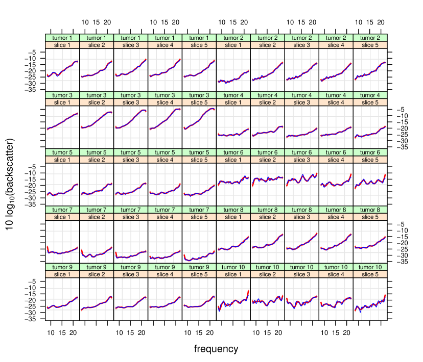
Figure 3: Illustrative three-level curve-type data with approximate fitted group specific curves and corresponding 99% credible sets based on mean field variational Bayes via Algorithm 4. The response variable is $10\log_{10}(\mbox{backscatter})$ according to ultrasound technology. Level 1 corresponds to different ultrasound frequencies and matches the horizontal axes in each panel. Level 2 corresponds to different slices of a tumor due to differing probe locations. Level 3 corresponds to different tumors with one tumor for each of $10$ laboratory mice.

4 Accuracy and Speed Assessment

In this section we provide some assessment of the accuracy and speed of the inference delivered by streamlined variational inference for group-specific curves models.

4.1 Accuracy Assessment

Mean field restrictions such as (12) and (24) imply that there is some loss of accuracy in inference produced by Algorithms 2 and 4. However, at least for the Gaussian response case treated here, approximate parameter orthogonality between the coefficient parameters and covariance parameters from likelihood theory implies that such restrictions are mild and mean field accuracy is high. Figure 4 corroborates this claim by assessing accuracy of the mean function estimates and 95% credible intervals at the median values of frequency for each panel in Figure 3. As a benchmark we use Markov chain Monte Carlo-based inference via the rstan package (Guo et al., 2018). After a warmup of size $1,000$ we retained $5,000$ Markov chain Monte Carlo samples from the mean function and median frequency posterior distributions and used kernel density estimation to approximate the corresponding posterior density function. For a generic univariate parameter $\theta$, the accuracy of an approximation $\mathfrak{q}(\theta)$ to $\mathfrak{p}(\theta|\boldsymbol{y})$ is defined to be

$$\mbox{accuracy}\equiv\,100\left\{1-{\textstyle{\frac{1}{2}}}\int_{-\infty}^{\infty}\big{|}\mathfrak{q}(\theta)-\mathfrak{p}(\theta|\boldsymbol{y})\big{|}\,d\theta\right\}\%.$$ (27)

The percentages in the top right-hand panel of Figure 4 correspond to (27) with replacement of $\mathfrak{p}(\theta|\boldsymbol{y})$ by the above-mentioned kernel density estimate. In this case accuracy is seen to be excellent, with accuracy percentages between 97% and 99% for all 40 curves.

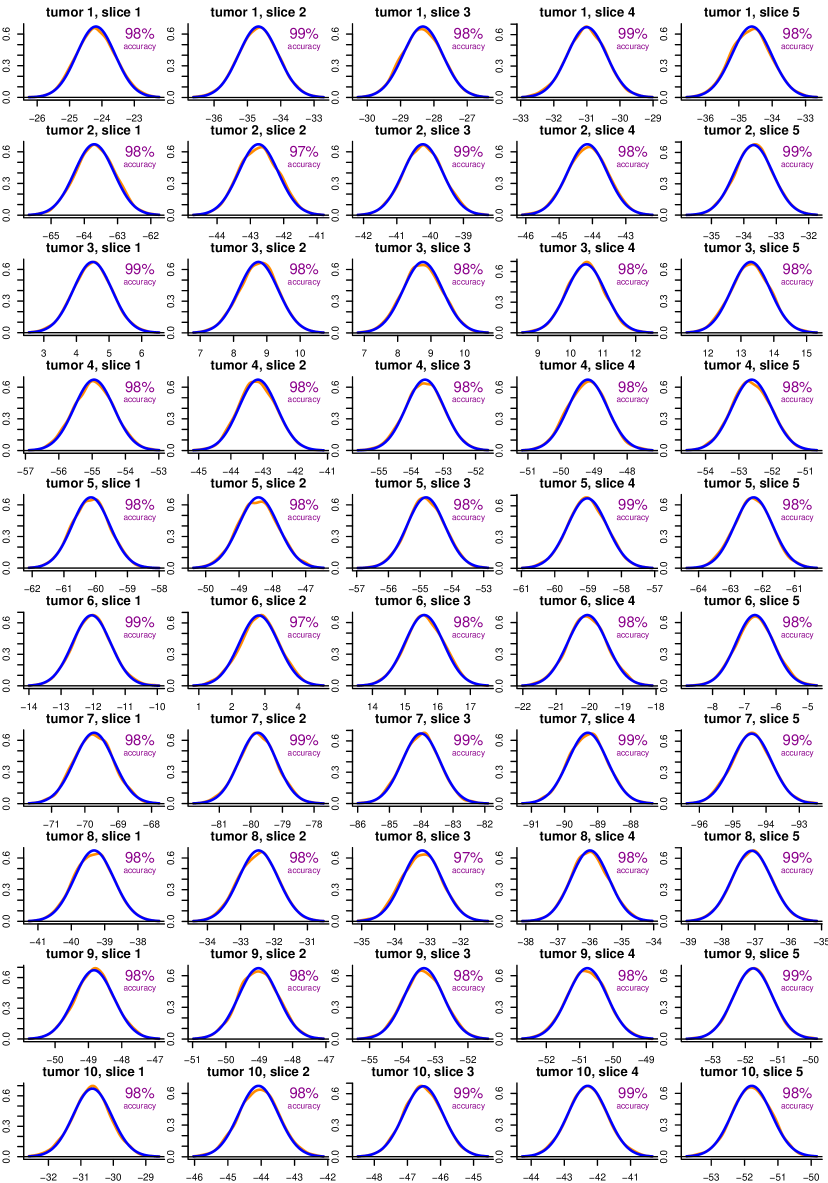
Figure 4: Accuracy assessment of Algorithm 4. Each panel displays approximate posterior density functions corresponding to mean function estimates according to the three-level group specific curve model (17). In each case the estimate is at the median frequency value. The orange density functions are based on Markov chain Monte Carlo and the blue density functions are based on mean field variational Bayes. The accuracy percentage scores are defined by (27).

4.2 Speed Assessment

We also conducted some simulation studies to assess the speed of streamlined variational higher level group-specific curve models, in terms of both comparative advantage over naïve implementation and absolute performance. The focus of these studies was variational inference in the two-level case and to probe maximal speed potential Algorithm 2 was implemented in the low-level computer language Fortran 77. An implementation of the naïve counterpart of Algorithm 2, involving storage and direct calculations concerning the full $\boldsymbol{\Sigma}_{\mathfrak{q}(\boldsymbol{\beta},\boldsymbol{u})}$ matrix, was also carried out. We then simulated data according to model (1) with $\sigma_{\varepsilon}=0.2$,

$$f(x)=3\sqrt{x(1.3-x)}\,\Phi(6x-3)\quad\mbox{and}\quad g_{i}(x)=\alpha_{1}\alpha_{2}\sin(2\pi x^{\alpha_{3}})$$

where, for each $i$, $\alpha_{1}$, $\alpha_{2}$ and $\alpha_{3}$ are, respectively, random draws from the $N({\textstyle{1\over 4}},{\textstyle{1\over 4}})$ distribution and the sets $\{-1,1\}$ and $\{1,2,3\}$. The level-2 sample sizes $n_{i}$ generated randomly from the set $\{30,31,\ldots,60\}$ and the level-1 sample sizes $m$ ranging over the set $\{100,200,300,400,500\}$. All $x_{ij}$ data were generated from a Uniform distribution over the unit interval. Table 1 summarizes the timings based on 100 replications with the number of mean field variational Bayes iterations fixed at 50. The study was run on a MacBook Air laptop with a 2.2 gigahertz processor and 8 gigabytes of random access memory.

$m$	naïve	streamlined	naïve/streamlined
100	75 (1.21)	0.748 (0.0334)	100
200	660 (7.72)	1.490 (0.0491)	442
300	2210 (22.00)	2.260 (0.0567)	974
400	5180 (92.20)	3.040 (0.0718)	1700
500	NA	3.780 (0.0593)	NA

Table 1: Average (standard deviation) of elapsed computing times in seconds for fitting model (1) naïvely versus with streamlining via Algorithm 2. The NA entries indicates non applicability due to the naïve computations not being feasible.

For $m$ ranging from $100$ to $400$ we see that the naïve to streamlined ratios increase from about $100$ to $1,700$. When $m=500$ the naïve implementation fails to run due to its excessive storage demands. In contrast, the streamlined fits are produced in about $3$ seconds. It is clear that streamlined variational inference is to be preferred and is the only option for large numbers of groups.

We then obtained timings for the streamlined algorithm for $m$ becoming much larger, taking on values $100$, $500$, $2,500$ and $12,500$. The iterations in Algorithm 2 were stopped when the relative increase in the marginal log-likelihood fell below $10^{-5}$. The average and standard deviation times in seconds over 100 replications are shown in Table 2. We see that the computational times are approximately linear in $m$. Even with twelve and a half thousand groups, Algorithm 2 is able to deliver fitting and inference on a contemporary laptop computer in about one and a half minutes.

$m=100$	$m=500$	$m=2,500$	$m=12,500$
0.635	2.900	16.90	95.00
(0.183)	(0.391)	(1.92)	(4.92)

Table 2: Average (standard deviation) of elapsed computing times in seconds for fitting model (1) with streamlining via Algorithm 2.

References

Atay-Kayis, A. & Massam, H. (2005). A Monte Carlo method for computing marginal likelihood in nondecomposable Gaussian graphical models. Biometrika, 92, 317–335.

Bates, D., Mächler, M., Bolker, B. and Walker, S. (2015). Fitting linear mixed-effects models using lme4. Journal of Statistical Software, 67(1), 1–48.

Bishop, C.M. (2006). Pattern Recognition and Machine Learning. New York: Springer.

Brumback, B.A. and Rice, J.A. (1998). Smoothing spline models for the analysis of nested and crossed samples of curves (with discussion). Journal of the American Statistical Association, 93, 961–994.

Donnelly, C.A., Laird, N.M. and Ware, J.H. (1995). Prediction and creation of smooth curves for temporally correlated longitudinal data. Journal of the American Statistical Association, 90, 984–989.

Durban, M., Harezlak, J., Wand, M.P. and Carroll, R.J. (2005). Simple fitting of subject-specific curves for longitudinal data. Statistics in Medicine, 24, 1153–1167.

Goldsmith, J., Zipunnikov, V. and Schrack, J. (2015). Generalized multilevel function-on-scalar regression and principal component analysis. Biometrics, 71, 344–353.

Guo, J., Gabry, J. and Goodrich, B. (2018). rstan: R interface to Stan. R package version 2.18.2.
http://mc-stan.org.

Huang, A. and Wand, M.P. (2013). Simple marginally noninformative prior distributions for covariance matrices. Bayesian Analysis, 8, 439–452.

Lee, C.Y.Y. and Wand, M.P. (2016). Variational inference for fitting complex Bayesian mixed effects models to health data. Statistics in Medicine, 35, 165–188.

Nolan, T.H., Menictas, M. and Wand, M.P. (2019). Streamlined computing for variational inference with higher level random effects. Unpublished manuscript submitted to the arXiv.org e-Print archive; on hold as of 11th March 2019. Soon to be posted also on http://matt-wand.utsacademics.info/statsPapers.html

Nolan, T.H. and Wand, M.P. (2018). Solutions to sparse multilevel matrix problems. Unpublished manuscript available at https://arxiv.org/abs/1903.03089.

Pinheiro, J.C. and Bates, D.M. (2000). Mixed-Effects Models in S and S-PLUS. New York: Springer.

Pinheiro, J., Bates, D., DebRoy, S., Sarkar, D. and R Core Team. (2018). nlme: Linear and nonlinear mixed effects models. R package version 3.1.
http://cran.r-project.org/package=nlme.

Pratt, J.H., Jones, J.J., Miller, J.Z., Wagner, M.A. and Fineberg, N.S. (1989). Racial differences in aldosterone excretion and plasma aldosterone concentrations in children. New England Journal of Medicine, 321, 1152–1157.

Robinson, G.K. (1991). That BLUP is a good thing: the estimation of random effects. Statistical Science, 6, 15–51.

Trail, J.B., Collins, L.M., Rivera, D.E., Li, R., Piper, M.E. and Baker, T.B. (2014). Functional data analysis for dynamical system identification of behavioral processes. Psychological Methods, 19(2), 175–187.

Verbyla, A.P., Cullis, B.R., Kenward, M.G. and Welham, S.J. (1999). The analysis of designed experiments and longitudinal data by using smoothing splines (with discussion). Applied Statistics, 48, 269–312.

Wahba, G. (1990). Spline Models for Observational Data. Philadelphia: Society for Industrial and Applied Mathematics.

Wand, M.P. and Ormerod, J.T. (2008). On semiparametric regression with O’Sullivan penalized splines. Australian and New Zealand Journal of Statistics, 50, 179–198.

Wand, M.P. and Ormerod, J.T. (2011). Penalized wavelets: embedding wavelets into semiparametric regression. Electronic Journal of Statistics, 5, 1654–1717.

Wang, Y. (1998). Mixed effects smoothing spline analysis of variance. Journal of the Royal Statistical Society, Series B, 60, 159–174.

Wirtzfeld, L.A., Ghoshal, G., Rosado-Mendez, I.M., Nam, K., Park, Y., Pawlicki, A.D., Miller, R.J., Simpson, D.G., Zagzebski, J.A., Oelze, M.I., Hall, T.J. and O’Brien, W.D. (2015). Quantitative ultrasound comparison of MAT and 4T1 mammary tumors in mice and rates across multiple imaging systems. Journal of Ultrasound Medicine, 34, 1373–1383.

Zhang, D., Lin, X., Raz, J. and Sowers, M. (1998). Semi-parametric stochastic mixed models for longitudinal data. Journal of the American Statistical Association, 93, 710–719.

Web-Supplement for:

Streamlined Variational Inference for

Higher Level Group-Specific Curve Models

By M. Menictas¹, T.H. Nolan¹, D.G. Simpson² and M.P. Wand¹

University of Technology Sydney¹ and University of Illinois²

S.1 Derivation of Result 1

Straightforward algebra can be used to verify that

$$\begin{array}[]{c}\boldsymbol{C}^{T}\boldsymbol{R}_{\mbox{{\bf BLUP}}}^{-1}\boldsymbol{C}+\boldsymbol{D}_{\mbox{{\bf BLUP}}}=\boldsymbol{B}^{T}\boldsymbol{B}\mbox{ and }\boldsymbol{C}^{T}\boldsymbol{R}_{\mbox{{\bf BLUP}}}^{-1}\boldsymbol{y}=\boldsymbol{B}^{T}\boldsymbol{b}\end{array}$$

where $\boldsymbol{B}$ and $\boldsymbol{b}$ have sparse forms (10) with non-zero sub-blocks equal to

$$\boldsymbol{b}_{i}\equiv\left[\begin{array}[]{c}\sigma_{\varepsilon}^{-1}\boldsymbol{y}_{i}\\[4.30554pt] \boldsymbol{0}\\[4.30554pt] \boldsymbol{0}\\[4.30554pt] \boldsymbol{0}\\[4.30554pt] \end{array}\right],\quad\boldsymbol{B}_{i}\equiv\left[\begin{array}[]{cc}\sigma_{\varepsilon}^{-1}\boldsymbol{X}_{i}&\sigma_{\varepsilon}^{-1}\boldsymbol{Z}_{\mbox{\rm\tiny gbl,$i$}}\\[4.30554pt] \boldsymbol{O}&m^{-1/2}\sigma_{\mbox{\rm\tiny gbl}}^{-1}\boldsymbol{I}_{K_{\mbox{\rm\tiny gbl}}}\\[4.30554pt] \boldsymbol{O}&\boldsymbol{O}\\[4.30554pt] \boldsymbol{O}&\boldsymbol{O}\\[4.30554pt] \end{array}\right]\quad\mbox{and}\quad\overset{\ \mbox{{$\bullet$}}}{\boldsymbol{B}}_{i}\equiv\left[\begin{array}[]{cc}\sigma_{\varepsilon}^{-1}\boldsymbol{X}_{i}&\sigma_{\varepsilon}^{-1}\boldsymbol{Z}_{\mbox{\rm\tiny grp,$i$}}\\[4.30554pt] \boldsymbol{O}&\boldsymbol{O}\\[4.30554pt] \boldsymbol{\Sigma}^{-1/2}&\boldsymbol{O}\\[4.30554pt] \boldsymbol{O}&\sigma_{\mbox{\rm\tiny grp}}^{-1}\boldsymbol{I}_{K_{\mbox{\rm\tiny grp}}}\end{array}\right].$$

Therefore, in view of (7) and (8),

$$\left[\begin{array}[]{c}{\widehat{\boldsymbol{\beta}}}\\ {\widehat{\boldsymbol{u}}}\end{array}\right]=(\boldsymbol{B}^{T}\boldsymbol{B})^{-1}\boldsymbol{B}^{T}\boldsymbol{b}\quad\mbox{and}\quad\mbox{\rm Cov}\left(\left[\begin{array}[]{c}{\widehat{\boldsymbol{\beta}}}\\ {\widehat{\boldsymbol{u}}}-\boldsymbol{u}\end{array}\right]\right)=(\boldsymbol{B}^{T}\boldsymbol{B})^{-1}.$$

S.2 Derivation of Algorithm 1

Algorithm 1 is simply a proceduralization of Result 1.

S.3 The Inverse G-Wishart and Inverse $\chi^{2}$ Distributions

The Inverse G-Wishart corresponds to the matrix inverses of random matrices that have a G-Wishart distribution (e.g. Atay-Kayis & Massam, 2005). For any positive integer $d$, let $G$ be an undirected graph with $d$ nodes labeled $1,\ldots,d$ and set $E$ consisting of sets of pairs of nodes that are connected by an edge. We say that the symmetric $d\times d$ matrix $\boldsymbol{M}$ respects $G$ if

$$\boldsymbol{M}_{ij}=0\quad\mbox{for all}\quad\{i,j\}\notin E.$$

A $d\times d$ random matrix $\boldsymbol{X}$ has an Inverse G-Wishart distribution with graph $G$ and parameters $\xi>0$ and symmetric $d\times d$ matrix $\boldsymbol{\Lambda}$, written

$$\boldsymbol{X}\sim\mbox{Inverse-G-Wishart}(G,\xi,\boldsymbol{\Lambda})$$

if and only if the density function of $\boldsymbol{X}$ satisfies

$$\mathfrak{p}(\boldsymbol{X})\propto|\boldsymbol{X}|^{-(\xi+2)/2}\exp\{-{\textstyle{\frac{1}{2}}}\mbox{tr}(\boldsymbol{\Lambda}\,\boldsymbol{X}^{-1})\}$$

over arguments $\boldsymbol{X}$ such that $\boldsymbol{X}$ is symmetric and positive definite and $\boldsymbol{X}^{-1}$ respects $G$. Two important special cases are

$$G=G_{\mbox{\rm\tiny full}}\equiv\mbox{totally connected $d$-node graph},$$

for which the Inverse G-Wishart distribution coincides with the ordinary Inverse Wishart distribution, and

$$G=G_{\mbox{\rm\tiny diag}}\equiv\mbox{totally disconnected $d$-node graph},$$

for which the Inverse G-Wishart distribution coincides with a product of independent Inverse Chi-Squared random variables. The subscripts of $G_{\mbox{\rm\tiny full}}$ and $G_{\mbox{\rm\tiny diag}}$ reflect the fact that $\boldsymbol{X}^{-1}$ is a full matrix and $\boldsymbol{X}^{-1}$ is a diagonal matrix in each special case.

The $G=G_{\mbox{\rm\tiny full}}$ case corresponds to the ordinary Inverse Wishart distribution. However, with message passing in mind, we will work with the more general Inverse G-Wishart family throughout this article.

In the $d=1$ special case the graph $G=G_{\mbox{\rm\tiny full}}=G_{\mbox{\rm\tiny diag}}$ and the Inverse G-Wishart distribution reduces to the Inverse Chi-Squared distributions. We write

$$x\sim\mbox{Inverse-$\chi^{2}$}(\xi,\lambda)$$

for this $\mbox{Inverse-G-Wishart}(G_{\mbox{\rm\tiny diag}},\xi,\lambda)$ special case with $d=1$ and $\lambda>0$ scalar.

S.4 Derivation of Result 2

It is straightforward to verify that the $\boldsymbol{\mu}_{\mathfrak{q}(\boldsymbol{\beta},\boldsymbol{u})}$ and $\boldsymbol{\Sigma}_{\mathfrak{q}(\boldsymbol{\beta},\boldsymbol{u})}$ updates, given at (13), may be written as

$$\boldsymbol{\mu}_{\mathfrak{q}(\boldsymbol{\beta},\boldsymbol{u})}\longleftarrow(\boldsymbol{B}^{T}\boldsymbol{B})^{-1}\boldsymbol{B}^{T}\boldsymbol{b}\quad\mbox{and}\quad\boldsymbol{\Sigma}_{\mathfrak{q}(\boldsymbol{\beta},\boldsymbol{u})}\longleftarrow(\boldsymbol{B}^{T}\boldsymbol{B})^{-1}$$

where $\boldsymbol{B}$ and $\boldsymbol{b}$ have the forms (10) with

$$\boldsymbol{b}_{i}\equiv\left[\begin{array}[]{c}\mu_{\mathfrak{q}(1/\sigma_{\varepsilon}^{2})}^{1/2}\boldsymbol{y}_{i}\\[8.61108pt] m^{-1/2}\boldsymbol{\Sigma}_{\boldsymbol{\beta}}^{-1/2}\boldsymbol{\mu}_{\boldsymbol{\beta}}\\[8.61108pt] \boldsymbol{0}\\[4.30554pt] \boldsymbol{0}\\[4.30554pt] \boldsymbol{0}\end{array}\right],\quad\boldsymbol{B}_{i}\equiv\left[\begin{array}[]{cc}\mu_{\mathfrak{q}(1/\sigma_{\varepsilon}^{2})}^{1/2}\boldsymbol{X}_{i}&\mu_{\mathfrak{q}(1/\sigma_{\varepsilon}^{2})}^{1/2}\boldsymbol{Z}_{\mbox{\rm\tiny gbl,$i$}}\\[8.61108pt] m^{-1/2}\boldsymbol{\Sigma}_{\boldsymbol{\beta}}^{-1/2}&\boldsymbol{O}\\[8.61108pt] \boldsymbol{O}&m^{-1/2}\mu_{\mathfrak{q}(1/\sigma_{\mbox{\rm\tiny gbl}}^{2})}^{1/2}\boldsymbol{I}_{K_{\mbox{\rm\tiny gbl}}}\\[8.61108pt] \boldsymbol{O}&\boldsymbol{O}\\[8.61108pt] \boldsymbol{O}&\boldsymbol{O}\\[8.61108pt] \end{array}\right]$$

and

$$\overset{\ \mbox{{$\bullet$}}}{\boldsymbol{B}}_{i}\equiv\left[\begin{array}[]{cc}\mu_{\mathfrak{q}(1/\sigma_{\varepsilon}^{2})}^{1/2}\boldsymbol{X}_{i}&\mu_{\mathfrak{q}(1/\sigma_{\varepsilon}^{2})}^{1/2}\boldsymbol{Z}_{\mbox{\rm\tiny grp,$i$}}\\[8.61108pt] \boldsymbol{O}&\boldsymbol{O}\\[8.61108pt] \boldsymbol{O}&\boldsymbol{O}\\[8.61108pt] \boldsymbol{M}_{\mathfrak{q}(\boldsymbol{\Sigma}^{-1})}^{1/2}&\boldsymbol{O}\\[8.61108pt] \boldsymbol{O}&\mu_{\mathfrak{q}(1/\sigma_{\mbox{\rm\tiny grp}}^{2})}^{1/2}\boldsymbol{I}_{K_{\mbox{\rm\tiny grp}}}\end{array}\right].$$

Result 2 immediately follows from Theorem 2 of Nolan & Wand (2018).

S.5 Derivation of Algorithm 2

We provide expressions for the $\mathfrak{q}$-densities for mean field variational Bayesian inference for the parameters in (11), with product density restriction (12). Arguments analogous to those given in, for example, Appendix C of Wand & Ormerod (2011) lead to:

$$\mathfrak{q}(\boldsymbol{\beta},\boldsymbol{u})\ \mbox{is a $N(\boldsymbol{\mu}_{\mathfrak{q}(\boldsymbol{\beta},\boldsymbol{u})},\boldsymbol{\Sigma}_{\mathfrak{q}(\boldsymbol{\beta},\boldsymbol{u})})$ density function}$$

where

$$\boldsymbol{\Sigma}_{\mathfrak{q}(\boldsymbol{\beta},\boldsymbol{u})}=(\boldsymbol{C}^{T}\boldsymbol{R}_{\mbox{{\bf MFVB}}}^{-1}\boldsymbol{C}+\boldsymbol{D}_{\mbox{{\bf MFVB}}})^{-1}\quad\mbox{and}\quad\boldsymbol{\mu}_{\mathfrak{q}(\boldsymbol{\beta},\boldsymbol{u})}=\boldsymbol{\Sigma}_{\mathfrak{q}(\boldsymbol{\beta},\boldsymbol{u})}(\boldsymbol{C}^{T}\boldsymbol{R}_{\mbox{{\bf MFVB}}}^{-1}\boldsymbol{y}+\boldsymbol{o}_{\mbox{{\bf MFVB}}})$$

with $\boldsymbol{R}_{\mbox{{\bf MFVB}}}$, $\boldsymbol{D}_{\mbox{{\bf MFVB}}}$ and $\boldsymbol{o}_{\mbox{{\bf MFVB}}}$ defined via (14),

$$\mathfrak{q}(\sigma_{\varepsilon}^{2})\ \mbox{is an $\mbox{Inverse-$\chi^{2}$}\left(\xi_{\mathfrak{q}(\sigma_{\varepsilon}^{2})},\lambda_{\mathfrak{q}(\sigma_{\varepsilon}^{2})}\right)$ density function}$$

where $\xi_{\mathfrak{q}(\sigma_{\varepsilon}^{2})}=\nu_{\varepsilon}+\sum_{i=1}^{m}n_{i}$ and

$$\lambda_{\mathfrak{q}(\sigma_{\varepsilon}^{2})} = \mu_{\mathfrak{q}(1/a_{\varepsilon})}+\sum_{i=1}^{m}\,E_{\mathfrak{q}}\left\{\Bigg{\|}\boldsymbol{y}_{i}-\boldsymbol{C}_{\mbox{\rm\tiny gbl,$i$}}\left[\begin{array}[]{c}\boldsymbol{\beta}\\[4.30554pt] \boldsymbol{u}_{\mbox{\rm\tiny gbl}}\end{array}\right]-\boldsymbol{C}_{\mbox{\rm\tiny grp,$i$}}\left[\begin{array}[]{c}\boldsymbol{u}_{\mbox{\rm\tiny lin,$i$}}\\[4.30554pt] \boldsymbol{u}_{\mbox{\rm\tiny grp,$i$}}\end{array}\right]\Bigg{\|}^{2}\right\}$$

$$= \mu_{\mathfrak{q}(1/a_{\varepsilon})}+\sum_{i=1}^{m}\,\left[\Bigg{\|}\,E_{\mathfrak{q}}\left(\boldsymbol{y}_{i}-\boldsymbol{C}_{\mbox{\rm\tiny gbl,$i$}}\left[\begin{array}[]{c}\boldsymbol{\beta}\\[4.30554pt] \boldsymbol{u}_{\mbox{\rm\tiny gbl}}\end{array}\right]-\boldsymbol{C}_{\mbox{\rm\tiny grp,$i$}}\left[\begin{array}[]{c}\boldsymbol{u}_{\mbox{\rm\tiny lin,$i$}}\\[4.30554pt] \boldsymbol{u}_{\mbox{\rm\tiny grp,$i$}}\end{array}\right]\right)\Bigg{\|}^{2}\right.$$

$$\left.\qquad\qquad\qquad\qquad+\mbox{tr}\left\{\mbox{\rm Cov}_{\mathfrak{q}}\left(\boldsymbol{C}_{\mbox{\rm\tiny gbl,$i$}}\left[\begin{array}[]{c}\boldsymbol{\beta}\\[4.30554pt] \boldsymbol{u}_{\mbox{\rm\tiny gbl,$i$}}\end{array}\right]+\boldsymbol{C}_{\mbox{\rm\tiny grp,$i$}}\left[\begin{array}[]{c}\boldsymbol{u}_{\mbox{\rm\tiny lin,$i$}}\\[4.30554pt] \boldsymbol{u}_{\mbox{\rm\tiny grp,$i$}}\end{array}\right]\right)\right\}\right]$$

$$= \mu_{\mathfrak{q}(1/a_{\varepsilon})}+\displaystyle{\sum_{i=1}^{m}}\left\{\Bigg{\|}E_{\mathfrak{q}}\left(\boldsymbol{y}_{i}-\boldsymbol{C}_{\mbox{\rm\tiny gbl,$i$}}\left[\begin{array}[]{c}\boldsymbol{\beta}\\[4.30554pt] \boldsymbol{u}_{\mbox{\rm\tiny gbl}}\end{array}\right]-\boldsymbol{C}_{\mbox{\rm\tiny grp,$i$}}\left[\begin{array}[]{c}\boldsymbol{u}_{\mbox{\rm\tiny lin,$i$}}\\[4.30554pt] \boldsymbol{u}_{\mbox{\rm\tiny grp,$i$}}\end{array}\right]\right)\Bigg{\|}^{2}\right.$$

$$\qquad\qquad\qquad\quad\left.+\mbox{tr}(\boldsymbol{C}_{\mbox{\rm\tiny gbl,$i$}}^{T}\boldsymbol{C}_{\mbox{\rm\tiny gbl,$i$}}\boldsymbol{\Sigma}_{\mathfrak{q}(\boldsymbol{\beta},\boldsymbol{u}_{\mbox{\rm\tiny gbl}})})+\mbox{tr}(\boldsymbol{C}_{\mbox{\rm\tiny grp,$i$}}^{T}\boldsymbol{C}_{\mbox{\rm\tiny grp,$i$}}\boldsymbol{\Sigma}_{\mathfrak{q}(\boldsymbol{u}_{\mbox{\rm\tiny lin,$i$}},\boldsymbol{u}_{\mbox{\rm\tiny grp,$i$}})})\right.$$

$$\qquad\qquad\qquad\quad\left.+2\,\mbox{tr}\left[\boldsymbol{C}_{\mbox{\rm\tiny grp,$i$}}^{T}\boldsymbol{C}_{\mbox{\rm\tiny gbl,$i$}}\,E_{\mathfrak{q}}\left\{\left(\left[\begin{array}[]{c}\boldsymbol{\beta}\\ \boldsymbol{u}_{\mbox{\rm\tiny gbl}}\end{array}\right]-\boldsymbol{\mu}_{\mathfrak{q}(\boldsymbol{\beta},\boldsymbol{u}_{\mbox{\rm\tiny gbl}})}\right)\times\right.\right.\right.$$

$$\left.\left.\left.\qquad\qquad\qquad\qquad\qquad\qquad\qquad\quad\quad\left(\left[\begin{array}[]{c}\boldsymbol{u}_{\mbox{\rm\tiny lin,$i$}}\\ \boldsymbol{u}_{\mbox{\rm\tiny grp,$i$}}\end{array}\right]-\boldsymbol{\mu}_{\mathfrak{q}(\boldsymbol{u}_{\mbox{\rm\tiny lin,$i$}},\boldsymbol{u}_{\mbox{\rm\tiny grp,$i$}})}\right)^{T}\right\}\right]\right\}$$

where $\boldsymbol{C}_{\mbox{\rm\tiny gbl,$i$}}\equiv[\boldsymbol{X}_{i}\,\boldsymbol{Z}_{\mbox{\rm\tiny gbl,$i$}}]$, $\boldsymbol{C}_{\mbox{\rm\tiny grp,$i$}}\equiv[\boldsymbol{X}_{i}\,\boldsymbol{Z}_{\mbox{\rm\tiny grp,$i$}}]$, and with reciprocal moment $\mu_{\mathfrak{q}(1/\sigma_{\varepsilon}^{2})}=\xi_{\mathfrak{q}(\sigma_{\varepsilon}^{2})}/\lambda_{\mathfrak{q}(\sigma_{\varepsilon}^{2})},$

$$\mathfrak{q}(\sigma_{\mbox{\rm\tiny gbl}}^{2})\ \mbox{is an $\mbox{Inverse-$\chi^{2}$}\left(\xi_{\mathfrak{q}(\sigma_{\mbox{\rm\tiny gbl}}^{2})},\lambda_{\mathfrak{q}(\sigma_{\mbox{\rm\tiny gbl}}^{2})}\right)$ density function}$$

where $\xi_{\mathfrak{q}(\sigma_{\mbox{\rm\tiny gbl}}^{2})}=\nu_{\mbox{\rm\tiny gbl}}+K_{\mbox{\rm\tiny gbl}}$ and

$$\lambda_{\mathfrak{q}(\sigma_{\mbox{\rm\tiny gbl}}^{2})}=\mu_{\mathfrak{q}(1/{a_{\mbox{\rm\tiny gbl}}})}+\|\boldsymbol{\mu}_{\mathfrak{q}(\boldsymbol{u}_{\mbox{\rm\tiny gbl}})}\|^{2}+\mbox{tr}\left(\boldsymbol{\Sigma}_{\mathfrak{q}(\boldsymbol{u}_{\mbox{\rm\tiny gbl}})}\right),$$

with reciprocal moment $\mu_{\mathfrak{q}(1/{\sigma_{\mbox{\rm\tiny gbl}}^{2}})}=\xi_{\mathfrak{q}(\sigma_{\mbox{\rm\tiny gbl}}^{2})}/\lambda_{\mathfrak{q}(\sigma_{\mbox{\rm\tiny gbl}}^{2})},$

$$\mathfrak{q}(\sigma_{\mbox{\rm\tiny grp}}^{2})\ \mbox{is an $\mbox{Inverse-$\chi^{2}$}\left(\xi_{\mathfrak{q}(\sigma_{\mbox{\rm\tiny grp}}^{2})},\lambda_{\mathfrak{q}(\sigma_{\mbox{\rm\tiny grp}}^{2})}\right)$ density function}$$

where $\xi_{\mathfrak{q}(\sigma_{\mbox{\rm\tiny grp}}^{2})}=\nu_{\mbox{\rm\tiny grp}}+mK_{\mbox{\rm\tiny grp}}$ and

$$\lambda_{\mathfrak{q}(\sigma_{\mbox{\rm\tiny grp}}^{2})}=\mu_{\mathfrak{q}(1/{a_{\mbox{\rm\tiny grp}}})}+\sum_{i=1}^{m}\left\{\|\boldsymbol{\mu}_{\mathfrak{q}(\boldsymbol{u}_{\mbox{\rm\tiny grp,$i$}})}\|^{2}+\mbox{tr}\left(\boldsymbol{\Sigma}_{\mathfrak{q}(\boldsymbol{u}_{\mbox{\rm\tiny grp,$i$}})}\right)\right\},$$

with reciprocal moment $\mu_{\mathfrak{q}(1/{\sigma_{\mbox{\rm\tiny grp}}^{2}})}=\xi_{\mathfrak{q}(\sigma_{\mbox{\rm\tiny grp}}^{2})}/\lambda_{\mathfrak{q}(\sigma_{\mbox{\rm\tiny grp}}^{2})},$

$$\mathfrak{q}(\boldsymbol{\Sigma})\ \mbox{is an $\mbox{Inverse-G-Wishart}\left(G_{\mbox{\rm\tiny full}},\xi_{\mathfrak{q}(\boldsymbol{\Sigma})},\boldsymbol{\Lambda}_{\mathfrak{q}(\boldsymbol{\Sigma})}\right)$ density function}$$

where $\xi_{\mathfrak{q}(\boldsymbol{\Sigma})}=\nu_{\mbox{\rm\tiny{$\boldsymbol{\Sigma}$}}}+2+m$

$$\boldsymbol{\Lambda}_{\mathfrak{q}(\boldsymbol{\Sigma})}=\boldsymbol{M}_{\mathfrak{q}(\boldsymbol{A}_{\boldsymbol{\Sigma}}^{-1})}+\sum_{i=1}^{m}\left(\boldsymbol{\mu}_{\mathfrak{q}(\boldsymbol{u}_{\mbox{\rm\tiny lin,$i$}})}\boldsymbol{\mu}_{\mathfrak{q}(\boldsymbol{u}_{\mbox{\rm\tiny lin,$i$}})}^{T}+\boldsymbol{\Sigma}_{\mathfrak{q}(\boldsymbol{u}_{\mbox{\rm\tiny lin,$i$}})}\right),$$

with inverse moment $\boldsymbol{M}_{\mathfrak{q}(\boldsymbol{\Sigma}^{-1})}=(\xi_{\mathfrak{q}(\boldsymbol{\Sigma})}-1)\boldsymbol{\Lambda}_{\mathfrak{q}(\boldsymbol{\Sigma})}^{-1}$,

$$\mathfrak{q}(a_{\varepsilon})\ \mbox{is an $\mbox{Inverse-$\chi^{2}$}(\xi_{\mathfrak{q}(a_{\varepsilon})},\lambda_{\mathfrak{q}(a_{\varepsilon})})$ density function}$$

where $\xi_{\mathfrak{q}(a_{\varepsilon})}=\nu_{\varepsilon}+1$,

$$\lambda_{\mathfrak{q}(a_{\varepsilon})}=\mu_{\mathfrak{q}(1/\sigma_{\varepsilon}^{2})}+1/(\nu_{\varepsilon}s_{\varepsilon}^{2})$$

with reciprocal moment $\mu_{\mathfrak{q}(1/a_{\varepsilon})}=\xi_{\mathfrak{q}(a_{\varepsilon})}/\lambda_{\mathfrak{q}(a_{\varepsilon})}$,

$$\mathfrak{q}(a_{\mbox{\rm\tiny gbl}})\ \mbox{is an $\mbox{Inverse-$\chi^{2}$}(\xi_{\mathfrak{q}(a_{\mbox{\rm\tiny gbl}})},\lambda_{\mathfrak{q}(a_{\mbox{\rm\tiny gbl}})})$ density function}$$

where $\xi_{\mathfrak{q}(a_{\mbox{\rm\tiny gbl}})}=\nu_{\mbox{\rm\tiny gbl}}+1$,

$$\lambda_{\mathfrak{q}(a_{\mbox{\rm\tiny gbl}})}=\mu_{\mathfrak{q}(1/\sigma_{\mbox{\rm\tiny gbl}}^{2})}+1/(\nu_{\mbox{\rm\tiny gbl}}s_{\mbox{\rm\tiny gbl}}^{2})$$

with reciprocal moment $\mu_{\mathfrak{q}(1/a_{\mbox{\rm\tiny gbl}})}=\xi_{\mathfrak{q}(a_{\mbox{\rm\tiny gbl}})}/\lambda_{\mathfrak{q}(a_{\mbox{\rm\tiny gbl}})}$,

$$\mathfrak{q}(a_{\mbox{\rm\tiny grp}})\ \mbox{is an $\mbox{Inverse-$\chi^{2}$}(\xi_{\mathfrak{q}(a_{\mbox{\rm\tiny grp}})},\lambda_{\mathfrak{q}(a_{\mbox{\rm\tiny grp}})})$ density function}$$

where $\xi_{\mathfrak{q}(a_{\mbox{\rm\tiny grp}})}=\nu_{\mbox{\rm\tiny grp}}+1$,

$$\lambda_{\mathfrak{q}(a_{\mbox{\rm\tiny grp}})}=\mu_{\mathfrak{q}(1/\sigma_{\mbox{\rm\tiny grp}}^{2})}+1/(\nu_{\mbox{\rm\tiny grp}}s_{\mbox{\rm\tiny grp}}^{2})$$

with reciprocal moment $\mu_{\mathfrak{q}(1/a_{\mbox{\rm\tiny grp}})}=\xi_{\mathfrak{q}(a_{\mbox{\rm\tiny grp}})}/\lambda_{\mathfrak{q}(a_{\mbox{\rm\tiny grp}})}$ and

$$\mathfrak{q}(\boldsymbol{A}_{\mbox{\rm\tiny$\boldsymbol{\Sigma}$}})\ \mbox{is an $\mbox{Inverse-G-Wishart}\left(G_{\mbox{\rm\tiny diag}},\xi_{\mathfrak{q}(\boldsymbol{A}_{\mbox{\rm\tiny$\boldsymbol{\Sigma}$}})},\boldsymbol{\Lambda}_{\mathfrak{q}(\boldsymbol{A}_{\mbox{\rm\tiny$\boldsymbol{\Sigma}$}})}\right)$ density function}$$

where $\xi_{\mathfrak{q}(\boldsymbol{A}_{\mbox{\rm\tiny$\boldsymbol{\Sigma}$}})}=\nu_{\mbox{\rm\tiny{$\boldsymbol{\Sigma}$}}}+2$,

$$\boldsymbol{\Lambda}_{\mathfrak{q}(\boldsymbol{A}_{\mbox{\rm\tiny$\boldsymbol{\Sigma}$}})}=\mbox{diag}\big{\{}\mbox{diagonal}\big{(}\boldsymbol{M}_{\mathfrak{q}(\boldsymbol{\Sigma}^{-1})}\big{)}\big{\}}+\boldsymbol{\Lambda}_{\boldsymbol{A}_{\mbox{\rm\tiny$\boldsymbol{\Sigma}$}}}$$

with inverse moment $\boldsymbol{M}_{\mathfrak{q}(\boldsymbol{A}_{\mbox{\rm\tiny$\boldsymbol{\Sigma}$}}^{-1})}=\xi_{\mathfrak{q}(\boldsymbol{A}_{\mbox{\rm\tiny$\boldsymbol{\Sigma}$}})}\boldsymbol{\Lambda}_{\mathfrak{q}(\boldsymbol{A}_{\mbox{\rm\tiny$\boldsymbol{\Sigma}$}})}^{-1}$.

S.6 Marginal Log-Likelihood Lower Bound and Derivation

The expression for the lower bound on the marginal log-likelihood for Algorithm 2 is

$$\begin{array}[]{l}\log\underline{\mathfrak{p}}(\boldsymbol{y};\mathfrak{q})=\\[8.61108pt] -\frac{1}{2}\log(\pi)\displaystyle{\sum_{i=1}^{m}}n_{i}-{\textstyle{\frac{1}{2}}}\log|\boldsymbol{\Sigma}_{\boldsymbol{\beta}}|-{\textstyle{\frac{1}{2}}}\mbox{tr}\left(\boldsymbol{\Sigma}_{\boldsymbol{\beta}}^{-1}\left\{\left(\boldsymbol{\mu}_{\mathfrak{q}(\boldsymbol{\beta})}-\boldsymbol{\mu}_{\boldsymbol{\beta}}\right)\left(\boldsymbol{\mu}_{\mathfrak{q}(\boldsymbol{\beta})}-\boldsymbol{\mu}_{\boldsymbol{\beta}}\right)^{T}+\boldsymbol{\Sigma}_{\mathfrak{q}(\boldsymbol{\beta})}\right\}\right)\\[4.30554pt] -{\textstyle{\frac{1}{2}}}\mbox{tr}\left(\boldsymbol{M}_{\mathfrak{q}(\boldsymbol{\Sigma}^{-1})}\left\{\displaystyle{\sum_{i=1}^{m}}\left(\boldsymbol{\mu}_{\mathfrak{q}(\boldsymbol{u}_{\mbox{\rm\tiny lin,$i$}}}\boldsymbol{\mu}_{\mathfrak{q}(\boldsymbol{u}_{\mbox{\rm\tiny lin,$i$}})}^{T}+\boldsymbol{\Sigma}_{\mathfrak{q}(\boldsymbol{u}_{\mbox{\rm\tiny lin,$i$}})}\right)\right\}\right)+{\textstyle{\frac{1}{2}}}\{2+K_{\mbox{\rm\tiny gbl}}+m(2+K_{\mbox{\rm\tiny grp}})\}\\[4.30554pt] -{\textstyle{\frac{1}{2}}}\mu_{\mathfrak{q}(1/{\sigma_{\mbox{\rm\tiny gbl}}^{2}})}\left\{\|\boldsymbol{\mu}_{\mathfrak{q}(\boldsymbol{u}_{\mbox{\rm\tiny gbl}})}\|^{2}+\mbox{tr}(\boldsymbol{\Sigma}_{\mathfrak{q}(\boldsymbol{u}_{\mbox{\rm\tiny gbl}})})\right\}-{\textstyle{\frac{1}{2}}}\mu_{\mathfrak{q}(1/{\sigma_{\mbox{\rm\tiny grp}}^{2}})}\displaystyle{\sum_{i=1}^{m}}\left\{\|\boldsymbol{\mu}_{\mathfrak{q}(\boldsymbol{u}_{\mbox{\rm\tiny grp,$i$}}))}\|^{2}+\mbox{tr}(\boldsymbol{\Sigma}_{\mathfrak{q}(\boldsymbol{u}_{\mbox{\rm\tiny grp,$i$}})})\right\}\\[4.30554pt] +{\textstyle{\frac{1}{2}}}\log|\boldsymbol{\Sigma}_{\boldsymbol{\beta}}|+\{\nu_{\mbox{\rm\tiny{$\boldsymbol{\Sigma}$}}}+m+1+{\textstyle{\frac{1}{2}}}(\nu_{\varepsilon}+\nu_{\mbox{\rm\tiny gbl}}+K_{\mbox{\rm\tiny gbl}}+\nu_{\mbox{\rm\tiny grp}}+mK_{\mbox{\rm\tiny grp}})\}\log(2)-\log\Gamma(\frac{\nu_{\varepsilon}}{2})\\[4.30554pt] -{\textstyle{\frac{1}{2}}}\mu_{\mathfrak{q}(1/{a_{\varepsilon}})}\mu_{\mathfrak{q}(1/{\sigma_{\varepsilon}^{2}})}-{\textstyle{\frac{1}{2}}}\xi_{\mathfrak{q}(\sigma_{\varepsilon}^{2})}\log(\lambda_{\mathfrak{q}(\sigma_{\varepsilon}^{2})})+\log\{\Gamma({\textstyle{\frac{1}{2}}}\xi_{\mathfrak{q}(\sigma_{\varepsilon}^{2})})\}+{\textstyle{\frac{1}{2}}}\lambda_{\mathfrak{q}(\sigma_{\varepsilon}^{2})}\mu_{\mathfrak{q}(1/\sigma_{\varepsilon}^{2})}-{\textstyle{\frac{1}{2}}}\log(\nu_{\varepsilon}s_{\varepsilon}^{2})\\[4.30554pt] -3\log\{\Gamma({\textstyle{\frac{1}{2}}})\}-\frac{1}{2\nu_{\varepsilon}s_{\varepsilon}^{2}}\mu_{\mathfrak{q}(1/a_{\varepsilon})}-{\textstyle{\frac{1}{2}}}\xi_{\mathfrak{q}(a_{\varepsilon})}\log(\lambda_{\mathfrak{q}(a_{\varepsilon})})+\log\{\Gamma({\textstyle{\frac{1}{2}}}\xi_{\mathfrak{q}(a_{\varepsilon})})\}+{\textstyle{\frac{1}{2}}}\lambda_{\mathfrak{q}(a_{\varepsilon})}\mu_{\mathfrak{q}(1/a_{\varepsilon})}\\[4.30554pt] -\log\Gamma(\frac{\nu_{\mbox{\rm\tiny gbl}}}{2})-{\textstyle{\frac{1}{2}}}\mu_{\mathfrak{q}(1/{a_{\mbox{\rm\tiny gbl}}})}\mu_{\mathfrak{q}(1/{\sigma_{\mbox{\rm\tiny gbl}}^{2}})}-{\textstyle{\frac{1}{2}}}\xi_{\mathfrak{q}(\sigma_{\mbox{\rm\tiny gbl}}^{2})}\log(\lambda_{\mathfrak{q}(\sigma_{\mbox{\rm\tiny gbl}}^{2})})+\log\{\Gamma({\textstyle{\frac{1}{2}}}\xi_{\mathfrak{q}(\sigma_{\mbox{\rm\tiny gbl}}^{2})})\}-{\textstyle{\frac{1}{2}}}\log(\nu_{\mbox{\rm\tiny gbl}}s_{\mbox{\rm\tiny gbl}}^{2})\\[4.30554pt] +{\textstyle{\frac{1}{2}}}\lambda_{\mathfrak{q}(\sigma_{\mbox{\rm\tiny gbl}}^{2})}\mu_{\mathfrak{q}(1/\sigma_{\mbox{\rm\tiny gbl}}^{2})}-\{1/(2\nu_{\mbox{\rm\tiny gbl}}s_{\mbox{\rm\tiny gbl}}^{2})\}\mu_{\mathfrak{q}(1/a_{\mbox{\rm\tiny gbl}})}-{\textstyle{\frac{1}{2}}}\xi_{\mathfrak{q}(a_{\mbox{\rm\tiny gbl}})}\log(\lambda_{\mathfrak{q}(a_{\mbox{\rm\tiny gbl}})})-{\textstyle{\frac{1}{2}}}\mu_{\mathfrak{q}(1/{a_{\mbox{\rm\tiny grp}}})}\mu_{\mathfrak{q}(1/{\sigma_{\mbox{\rm\tiny grp}}^{2}})}\\[4.30554pt] +\log\{\Gamma({\textstyle{\frac{1}{2}}}\xi_{\mathfrak{q}(a_{\mbox{\rm\tiny gbl}})})\}+{\textstyle{\frac{1}{2}}}\lambda_{\mathfrak{q}(a_{\mbox{\rm\tiny gbl}})}\mu_{\mathfrak{q}(1/a_{\mbox{\rm\tiny gbl}})}-\log\Gamma(\frac{\nu_{\mbox{\rm\tiny grp}}}{2})+\log\{\Gamma({\textstyle{\frac{1}{2}}}\xi_{\mathfrak{q}(\sigma_{\mbox{\rm\tiny grp}}^{2})})\}-{\textstyle{\frac{1}{2}}}\log(\nu_{\mbox{\rm\tiny grp}}s_{\mbox{\rm\tiny grp}}^{2})\\[4.30554pt] -{\textstyle{\frac{1}{2}}}\xi_{\mathfrak{q}(\sigma_{\mbox{\rm\tiny grp}}^{2})}\log(\lambda_{\mathfrak{q}(\sigma_{\mbox{\rm\tiny grp}}^{2})})+{\textstyle{\frac{1}{2}}}\lambda_{\mathfrak{q}(\sigma_{\mbox{\rm\tiny grp}}^{2})}\mu_{\mathfrak{q}(1/\sigma_{\mbox{\rm\tiny grp}}^{2})}-\{1/(2\nu_{\mbox{\rm\tiny grp}}s_{\mbox{\rm\tiny grp}}^{2})\}\mu_{\mathfrak{q}(1/a_{\mbox{\rm\tiny grp}})}-{\textstyle{\frac{1}{2}}}\xi_{\mathfrak{q}(a_{\mbox{\rm\tiny grp}})}\log(\lambda_{\mathfrak{q}(a_{\mbox{\rm\tiny grp}})})\\[4.30554pt] +\log\{\Gamma({\textstyle{\frac{1}{2}}}\xi_{\mathfrak{q}(a_{\mbox{\rm\tiny grp}})})\}+{\textstyle{\frac{1}{2}}}\lambda_{\mathfrak{q}(a_{\mbox{\rm\tiny grp}})}\mu_{\mathfrak{q}(1/a_{\mbox{\rm\tiny grp}})}-{\textstyle{\frac{1}{2}}}\mbox{tr}(\boldsymbol{M}_{\mathfrak{q}(\boldsymbol{A}_{\mbox{\rm\tiny$\boldsymbol{\Sigma}$}}^{-1})}\boldsymbol{M}_{\mathfrak{q}(\boldsymbol{\Sigma}^{-1})})+{\textstyle{\frac{1}{2}}}\mbox{tr}(\boldsymbol{\Lambda}_{\mathfrak{q}(\boldsymbol{\Sigma})}\boldsymbol{M}_{\mathfrak{q}(\boldsymbol{\Sigma}^{-1})})\\[4.30554pt] +\displaystyle{\sum_{j=1}^{2}}\log\Gamma({\textstyle{\frac{1}{2}}}(\xi_{\mathfrak{q}(\boldsymbol{A}_{\mbox{\rm\tiny$\boldsymbol{\Sigma}$}})}+2-j))-\displaystyle{\sum_{j=1}^{2}}\log\Gamma({\textstyle{\frac{1}{2}}}(\nu_{\mbox{\rm\tiny{$\boldsymbol{\Sigma}$}}}+4-j))-{\textstyle{\frac{1}{2}}}(\xi_{\mathfrak{q}(\boldsymbol{\Sigma})}-1)\log|\boldsymbol{\Lambda}_{\mathfrak{q}(\boldsymbol{\Sigma})}|\\[4.30554pt] +\displaystyle{\sum_{j=1}^{2}}\log\Gamma({\textstyle{\frac{1}{2}}}(\xi_{\mathfrak{q}(\boldsymbol{\Sigma})}+2-j))-{\textstyle{\frac{1}{2}}}\displaystyle{\sum_{j=1}^{2}}1/(\nu_{\mbox{\rm\tiny{$\boldsymbol{\Sigma}$}}}s_{\mbox{\rm\tiny{$\boldsymbol{\Sigma},j$}}}^{2})\left(\boldsymbol{M}_{\mathfrak{q}(\boldsymbol{A}_{\mbox{\rm\tiny$\boldsymbol{\Sigma}$}}^{-1})}\right)_{jj}-\displaystyle{\sum_{j=1}^{2}}\log\Gamma({\textstyle{\frac{1}{2}}}(3-j))\\[4.30554pt] -{\textstyle{\frac{1}{2}}}(\xi_{\mathfrak{q}(\boldsymbol{A}_{\mbox{\rm\tiny$\boldsymbol{\Sigma}$}})}-1)\log|\boldsymbol{\Lambda}_{\mathfrak{q}(\boldsymbol{A}_{\mbox{\rm\tiny$\boldsymbol{\Sigma}$}})}|+{\textstyle{\frac{1}{2}}}\mbox{tr}(\boldsymbol{\Lambda}_{\mathfrak{q}(\boldsymbol{A}_{\mbox{\rm\tiny$\boldsymbol{\Sigma}$}})}\boldsymbol{M}_{\mathfrak{q}(\boldsymbol{A}_{\mbox{\rm\tiny$\boldsymbol{\Sigma}$}}^{-1})})\\[4.30554pt] -\frac{1}{2}\mu_{\mathfrak{q}(1/{\sigma_{\varepsilon}^{2}})}\displaystyle{\sum_{i=1}^{m}}\left\{\Bigg{\|}E_{\mathfrak{q}}\left(\boldsymbol{y}_{i}-\boldsymbol{C}_{\mbox{\rm\tiny gbl,$i$}}\left[\begin{array}[]{c}\boldsymbol{\beta}\\[4.30554pt] \boldsymbol{u}_{\mbox{\rm\tiny gbl,$i$}}\end{array}\right]-\boldsymbol{C}_{\mbox{\rm\tiny grp,$i$}}\left[\begin{array}[]{c}\boldsymbol{u}_{\mbox{\rm\tiny lin,$i$}}\\[4.30554pt] \boldsymbol{u}_{\mbox{\rm\tiny grp,$i$}}\end{array}\right]\right)\Bigg{\|}^{2}\right.\\[12.91663pt] \qquad\qquad\qquad\quad\left.+\mbox{tr}(\boldsymbol{C}_{\mbox{\rm\tiny gbl,$i$}}^{T}\boldsymbol{C}_{\mbox{\rm\tiny gbl,$i$}}\boldsymbol{\Sigma}_{\mathfrak{q}(\boldsymbol{\beta},\boldsymbol{u}_{\mbox{\rm\tiny gbl}})})+\mbox{tr}(\boldsymbol{C}_{\mbox{\rm\tiny grp,$i$}}^{T}\boldsymbol{C}_{\mbox{\rm\tiny grp,$i$}}\boldsymbol{\Sigma}_{\mathfrak{q}(\boldsymbol{u}_{\mbox{\rm\tiny lin,$i$}},\boldsymbol{u}_{\mbox{\rm\tiny grp,$i$}})})\right.\\[4.30554pt] \qquad\qquad\qquad\quad\left.+2\,\mbox{tr}\left[\boldsymbol{C}_{\mbox{\rm\tiny grp,$i$}}^{T}\boldsymbol{C}_{\mbox{\rm\tiny gbl,$i$}}\,E_{\mathfrak{q}}\left\{\left(\left[\begin{array}[]{c}\boldsymbol{\beta}\\ \boldsymbol{u}_{\mbox{\rm\tiny gbl}}\end{array}\right]-\boldsymbol{\mu}_{\mathfrak{q}(\boldsymbol{\beta},\boldsymbol{u}_{\mbox{\rm\tiny gbl}})}\right)\times\right.\right.\right.\\[4.30554pt] \qquad\qquad\qquad\qquad\qquad\qquad\qquad\qquad\left.\left.\left.\left(\left[\begin{array}[]{c}\boldsymbol{u}_{\mbox{\rm\tiny lin,$i$}}\\ \boldsymbol{u}_{\mbox{\rm\tiny grp,$i$}}\end{array}\right]-\boldsymbol{\mu}_{\mathfrak{q}(\boldsymbol{u}_{\mbox{\rm\tiny lin,$i$}},\boldsymbol{u}_{\mbox{\rm\tiny grp,$i$}}))}\right)^{T}\right\}\right]\right\}.\end{array}$$ (S.7)

Derivation: The lower-bound on the marginal log-likelihood is achieved through the following expression:

$$\begin{array}[]{lcl}\log\underline{\mathfrak{p}}(\boldsymbol{y};\mathfrak{q})&=&E_{\mathfrak{q}}\{\log\mathfrak{p}(\boldsymbol{y},\boldsymbol{\beta},\boldsymbol{u},\sigma_{\varepsilon}^{2},a_{\varepsilon},\sigma_{\mbox{\rm\tiny gbl}}^{2},a_{\mbox{\rm\tiny gbl}},\sigma_{\mbox{\rm\tiny grp}}^{2},a_{\mbox{\rm\tiny grp}},\boldsymbol{\Sigma},\boldsymbol{A}_{\mbox{\rm\tiny$\boldsymbol{\Sigma}$}})\\[4.30554pt] &&-\,\log\mathfrak{q}^{*}(\boldsymbol{\beta},\boldsymbol{u},\sigma_{\varepsilon}^{2},a_{\varepsilon},\sigma_{\mbox{\rm\tiny gbl}}^{2},a_{\mbox{\rm\tiny gbl}},\sigma_{\mbox{\rm\tiny grp}}^{2},a_{\mbox{\rm\tiny grp}},\boldsymbol{\Sigma},\boldsymbol{A}_{\mbox{\rm\tiny$\boldsymbol{\Sigma}$}})\}\end{array}$$

$$\begin{array}[]{lcl}&=&E_{\mathfrak{q}}\{\log\mathfrak{p}(\boldsymbol{y}\,|\,\boldsymbol{\beta},\boldsymbol{u},\sigma_{\varepsilon}^{2})\}\\[4.30554pt] &&+\,E_{\mathfrak{q}}\{\log\mathfrak{p}(\boldsymbol{\beta},\boldsymbol{u}\,|\,\sigma_{\mbox{\rm\tiny gbl}}^{2},\sigma_{\mbox{\rm\tiny grp}}^{2},\boldsymbol{\Sigma})\}-E_{\mathfrak{q}}\{\log\mathfrak{q}^{*}(\boldsymbol{\beta},\boldsymbol{u})\}\\[4.30554pt] &&+\,E_{\mathfrak{q}}\{\log\mathfrak{p}(\sigma_{\varepsilon}^{2}\,|\,a_{\varepsilon})\}-E_{\mathfrak{q}}\{\log\mathfrak{q}^{*}(\sigma_{\varepsilon}^{2})\}+E_{\mathfrak{q}}\{\log\mathfrak{p}(a_{\varepsilon})\}-E_{\mathfrak{q}}\{\log\mathfrak{q}^{*}(a_{\varepsilon})\}\\[4.30554pt] &&+\,E_{\mathfrak{q}}\{\log\mathfrak{p}(\sigma_{\mbox{\rm\tiny gbl}}^{2}\,|\,a_{\mbox{\rm\tiny gbl}})\}-E_{\mathfrak{q}}\{\log\mathfrak{q}^{*}(\sigma_{\mbox{\rm\tiny gbl}}^{2})\}+E_{\mathfrak{q}}\{\log\mathfrak{p}(a_{\mbox{\rm\tiny gbl}})\}-E_{\mathfrak{q}}\{\log\mathfrak{q}^{*}(a_{\mbox{\rm\tiny gbl}})\}\\[4.30554pt] &&+\,E_{\mathfrak{q}}\{\log\mathfrak{p}(\sigma_{\mbox{\rm\tiny grp}}^{2}\,|\,a_{\mbox{\rm\tiny grp}})\}-E_{\mathfrak{q}}\{\log\mathfrak{q}^{*}(\sigma_{\mbox{\rm\tiny grp}}^{2})\}+E_{\mathfrak{q}}\{\log\mathfrak{p}(a_{\mbox{\rm\tiny grp}})\}-E_{\mathfrak{q}}\{\log\mathfrak{q}^{*}(a_{\mbox{\rm\tiny grp}})\}\\[4.30554pt] &&+\,E_{\mathfrak{q}}\{\log\mathfrak{p}(\boldsymbol{\Sigma}\,|\,\boldsymbol{A}_{\mbox{\rm\tiny$\boldsymbol{\Sigma}$}})\}-E_{\mathfrak{q}}\{\log\mathfrak{q}^{*}(\boldsymbol{\Sigma})\}+E_{\mathfrak{q}}\{\log\mathfrak{p}(\boldsymbol{A}_{\mbox{\rm\tiny$\boldsymbol{\Sigma}$}})\}-E_{\mathfrak{q}}\{\log\mathfrak{q}^{*}(\boldsymbol{A}_{\mbox{\rm\tiny$\boldsymbol{\Sigma}$}})\}.\end{array}$$ (S.8)

First we note that

$$\log\mathfrak{p}(\boldsymbol{y}\,|\,\boldsymbol{\beta},\boldsymbol{u},\sigma_{\varepsilon}^{2})=-\frac{1}{2}\log(2\pi)\displaystyle{\sum_{i=1}^{m}}n_{i}-\frac{1}{2}\log(\sigma_{\varepsilon}^{2})\displaystyle{\sum_{i=1}^{m}}n_{i}-\frac{1}{2\sigma_{\varepsilon}^{2}}\displaystyle{\sum_{i=1}^{m}}\|\boldsymbol{y}-\boldsymbol{X}\boldsymbol{\beta}-\boldsymbol{Z}\boldsymbol{u}\|^{2}$$

where

$$\begin{array}[]{l}\|\boldsymbol{y}-\boldsymbol{X}\boldsymbol{\beta}-\boldsymbol{Z}\boldsymbol{u}\|^{2}\\[4.30554pt] \quad=\bBigg@{4}\|\left[\begin{array}[]{c}\boldsymbol{y}_{1}\\ \vdots\\ \boldsymbol{y}_{m}\end{array}\right]-\left[\begin{array}[]{c}\boldsymbol{X}_{1}\\ \vdots\\ \boldsymbol{X}_{m}\end{array}\right]\boldsymbol{\beta}-\left[\begin{array}[]{c}\boldsymbol{Z}_{\mbox{\rm\tiny gbl,$1$}}\\ \vdots\\ \boldsymbol{Z}_{\mbox{\rm\tiny gbl,$m$}}\end{array}\right]\boldsymbol{u}_{\mbox{\rm\tiny gbl}}-\displaystyle\mathop{\mbox{\rm blockdiag}}_{1\leq i\leq m}([\boldsymbol{X}_{i}\ \boldsymbol{Z}_{\mbox{\rm\tiny grp,$i$}}])\left[\begin{array}[]{c}\boldsymbol{u}_{\mbox{\rm\tiny lin,$i$}}\\ \boldsymbol{u}_{\mbox{\rm\tiny grp,$i$}}\end{array}\right]_{1\leq i\leq m}\bBigg@{4}\|^{2}\\[21.52771pt] \quad=\displaystyle\sum_{i=1}^{m}\|\boldsymbol{y}_{i}-\boldsymbol{X}_{i}\boldsymbol{\beta}-\boldsymbol{Z}_{\mbox{\rm\tiny gbl,$i$}}\boldsymbol{u}_{\mbox{\rm\tiny gbl,$i$}}-\boldsymbol{X}_{i}\boldsymbol{u}_{\mbox{\rm\tiny lin,$i$}}-\boldsymbol{Z}_{\mbox{\rm\tiny grp,$i$}}\boldsymbol{u}_{\mbox{\rm\tiny grp,$i$}}\|^{2}\\[12.91663pt] \quad=\displaystyle\sum_{i=1}^{m}\Bigg{\|}\boldsymbol{y}_{i}-\boldsymbol{C}_{\mbox{\rm\tiny gbl,$i$}}\left[\begin{array}[]{c}\boldsymbol{\beta}\\[4.30554pt] \boldsymbol{u}_{\mbox{\rm\tiny gbl,$i$}}\end{array}\right]-\boldsymbol{C}_{\mbox{\rm\tiny grp,$i$}}\left[\begin{array}[]{c}\boldsymbol{u}_{\mbox{\rm\tiny lin,$i$}}\\[4.30554pt] \boldsymbol{u}_{\mbox{\rm\tiny grp,$i$}}\end{array}\right]\Bigg{\|}^{2}\end{array}$$

and

$$\begin{array}[]{c}\boldsymbol{C}_{\mbox{\rm\tiny gbl,$i$}}\equiv[\boldsymbol{X}_{i}\,\boldsymbol{Z}_{\mbox{\rm\tiny gbl,$i$}}],\quad\boldsymbol{C}_{\mbox{\rm\tiny grp,$i$}}\equiv[\boldsymbol{X}_{i}\,\boldsymbol{Z}_{\mbox{\rm\tiny grp,$i$}}].\end{array}$$

Therefore,

$$\begin{array}[]{l}E_{\mathfrak{q}}\{\log\mathfrak{p}(\boldsymbol{y}\,|\,\boldsymbol{\beta},\boldsymbol{u},\sigma_{\varepsilon}^{2})\}\\[4.30554pt] \quad=-\frac{1}{2}\log(2\pi)\displaystyle{\sum_{i=1}^{m}}n_{i}-\frac{1}{2}E_{\mathfrak{q}}\{\log(\sigma_{\varepsilon}^{2})\}\displaystyle{\sum_{i=1}^{m}}n_{i}\\[4.30554pt] \quad\quad-\frac{1}{2}\mu_{\mathfrak{q}(1/{\sigma_{\varepsilon}^{2}})}\displaystyle{\sum_{i=1}^{m}}\left\{\Bigg{\|}E_{\mathfrak{q}}\left(\boldsymbol{y}_{i}-\boldsymbol{C}_{\mbox{\rm\tiny gbl,$i$}}\left[\begin{array}[]{c}\boldsymbol{\beta}\\[4.30554pt] \boldsymbol{u}_{\mbox{\rm\tiny gbl,$i$}}\end{array}\right]-\boldsymbol{C}_{\mbox{\rm\tiny grp,$i$}}\left[\begin{array}[]{c}\boldsymbol{u}_{\mbox{\rm\tiny lin,$i$}}\\[4.30554pt] \boldsymbol{u}_{\mbox{\rm\tiny grp,$i$}}\end{array}\right]\right)\Bigg{\|}^{2}\right.\\[12.91663pt] \quad\quad\quad\left.+\mbox{tr}(\boldsymbol{C}_{\mbox{\rm\tiny gbl,$i$}}^{T}\boldsymbol{C}_{\mbox{\rm\tiny gbl,$i$}}\boldsymbol{\Sigma}_{\mathfrak{q}(\boldsymbol{\beta},\boldsymbol{u}_{\mbox{\rm\tiny gbl}})})+\mbox{tr}(\boldsymbol{C}_{\mbox{\rm\tiny grp,$i$}}^{T}\boldsymbol{C}_{\mbox{\rm\tiny grp,$i$}}\boldsymbol{\Sigma}_{\mathfrak{q}(\boldsymbol{u}_{\mbox{\rm\tiny lin,$i$}},\boldsymbol{u}_{\mbox{\rm\tiny grp,$i$}})})\right.\\[4.30554pt] \quad\quad\quad\left.+2\,\mbox{tr}\left[\boldsymbol{C}_{\mbox{\rm\tiny grp,$i$}}^{T}\boldsymbol{C}_{\mbox{\rm\tiny gbl,$i$}}\,E_{\mathfrak{q}}\left\{\left(\left[\begin{array}[]{c}\boldsymbol{\beta}\\ \boldsymbol{u}_{\mbox{\rm\tiny gbl}}\end{array}\right]-\boldsymbol{\mu}_{\mathfrak{q}(\boldsymbol{\beta},\boldsymbol{u}_{\mbox{\rm\tiny gbl}})}\right)\left(\left[\begin{array}[]{c}\boldsymbol{u}_{\mbox{\rm\tiny lin,$i$}}\\ \boldsymbol{u}_{\mbox{\rm\tiny grp,$i$}}\end{array}\right]-\boldsymbol{\mu}_{\mathfrak{q}(\boldsymbol{u}_{\mbox{\rm\tiny lin,$i$}},\boldsymbol{u}_{\mbox{\rm\tiny grp,$i$}}))}\right)^{T}\right\}\right]\right\}\end{array}$$

The remainder of the expectations in (S.8) are expressed as:

$$\begin{array}[]{lcl}E_{\mathfrak{q}}\{\log\mathfrak{p}(\boldsymbol{\beta},\boldsymbol{u}\,|\,\sigma_{\mbox{\rm\tiny gbl}}^{2},\sigma_{\mbox{\rm\tiny grp}}^{2},\boldsymbol{\Sigma})\}&=&-{\textstyle{\frac{1}{2}}}\{2+K_{\mbox{\rm\tiny gbl}}+m(2+K_{\mbox{\rm\tiny grp}})\}\log(2\pi)-{\textstyle{\frac{1}{2}}}\log|\boldsymbol{\Sigma}_{\boldsymbol{\beta}}|\\[4.30554pt] &&-\frac{K_{\mbox{\rm\tiny gbl}}}{2}E_{\mathfrak{q}}\{\log(\sigma_{\mbox{\rm\tiny gbl}}^{2})\}-\frac{m}{2}E_{\mathfrak{q}}\{\log|\boldsymbol{\Sigma}|\}-\frac{mK_{\mbox{\rm\tiny grp}}}{2}E_{\mathfrak{q}}\{\log(\sigma_{\mbox{\rm\tiny grp}}^{2})\}\\[4.30554pt] &&-{\textstyle{\frac{1}{2}}}\mbox{tr}\left(\boldsymbol{\Sigma}_{\boldsymbol{\beta}}^{-1}\left\{\left(\boldsymbol{\mu}_{\mathfrak{q}(\boldsymbol{\beta})}-\boldsymbol{\mu}_{\boldsymbol{\beta}}\right)\left(\boldsymbol{\mu}_{\mathfrak{q}(\boldsymbol{\beta})}-\boldsymbol{\mu}_{\boldsymbol{\beta}}\right)^{T}+\boldsymbol{\Sigma}_{\mathfrak{q}(\boldsymbol{\beta})}\right\}\right)\\[4.30554pt] &&-{\textstyle{\frac{1}{2}}}\mu_{\mathfrak{q}(1/{\sigma_{\mbox{\rm\tiny gbl}}^{2}})}\left\{\|\boldsymbol{\mu}_{\mathfrak{q}(\boldsymbol{u}_{\mbox{\rm\tiny gbl}})}\|^{2}+\mbox{tr}(\boldsymbol{\Sigma}_{\mathfrak{q}(\boldsymbol{u}_{\mbox{\rm\tiny gbl}})})\right\}\\[4.30554pt] &&-{\textstyle{\frac{1}{2}}}\mbox{tr}\left(\boldsymbol{M}_{\mathfrak{q}(\boldsymbol{\Sigma}^{-1})}\left\{\displaystyle{\sum_{i=1}^{m}}\left(\boldsymbol{\mu}_{\mathfrak{q}(\boldsymbol{u}_{\mbox{\rm\tiny lin,$i$}}}\boldsymbol{\mu}_{\mathfrak{q}(\boldsymbol{u}_{\mbox{\rm\tiny lin,$i$}})}^{T}+\boldsymbol{\Sigma}_{\mathfrak{q}(\boldsymbol{u}_{\mbox{\rm\tiny lin,$i$}})}\right)\right\}\right)\\[4.30554pt] &&-{\textstyle{\frac{1}{2}}}\mu_{\mathfrak{q}(1/{\sigma_{\mbox{\rm\tiny grp}}^{2}})}\displaystyle{\sum_{i=1}^{m}}\left\{\|\boldsymbol{\mu}_{\mathfrak{q}(\boldsymbol{u}_{\mbox{\rm\tiny grp,$i$}}))}\|^{2}+\mbox{tr}(\boldsymbol{\Sigma}_{\mathfrak{q}(\boldsymbol{u}_{\mbox{\rm\tiny grp,$i$}})})\right\}\end{array}$$

$$\begin{array}[]{lcl}E_{\mathfrak{q}}\{\log\mathfrak{q}^{*}(\boldsymbol{\beta},\boldsymbol{u})\}&=&-{\textstyle{\frac{1}{2}}}\{2+K_{\mbox{\rm\tiny gbl}}+m(2+K_{\mbox{\rm\tiny grp}})\}-{\textstyle{\frac{1}{2}}}\{2+K_{\mbox{\rm\tiny gbl}}+m(2+K_{\mbox{\rm\tiny grp}})\}\log(2\pi)\\[4.30554pt] &&-{\textstyle{\frac{1}{2}}}\log|\boldsymbol{\Sigma}_{\boldsymbol{\beta}}|\end{array}$$

$$\begin{array}[]{lcl}E_{\mathfrak{q}}\{\log\mathfrak{p}(\sigma_{\varepsilon}^{2}\,|\,a_{\varepsilon})\}&=&-{\textstyle{\frac{1}{2}}}\nu_{\varepsilon}E_{\mathfrak{q}}\{\log(2a_{\varepsilon})\}-\log\Gamma(\nu_{\varepsilon}/2)-({\textstyle{\frac{1}{2}}}\nu_{\varepsilon}+1)E_{\mathfrak{q}}\{\log(\sigma_{\varepsilon}^{2})\}\\[4.30554pt] &&-{\textstyle{\frac{1}{2}}}\mu_{\mathfrak{q}(1/{a_{\varepsilon}})}\mu_{\mathfrak{q}(1/{\sigma_{\varepsilon}^{2}})}\end{array}$$

$$\begin{array}[]{lcl}E_{\mathfrak{q}}\{\log\mathfrak{q}^{*}(\sigma_{\varepsilon}^{2})\}&=&{\textstyle{\frac{1}{2}}}\xi_{\mathfrak{q}(\sigma_{\varepsilon}^{2})}\log(\lambda_{\mathfrak{q}(\sigma_{\varepsilon}^{2})}/2)-\log\{\Gamma({\textstyle{\frac{1}{2}}}\xi_{\mathfrak{q}(\sigma_{\varepsilon}^{2})})\}-({\textstyle{\frac{1}{2}}}\xi_{\mathfrak{q}(\sigma_{\varepsilon}^{2})}+1)E_{\mathfrak{q}}\{\log(\sigma_{\varepsilon}^{2})\}\\[4.30554pt] &&-{\textstyle{\frac{1}{2}}}\lambda_{\mathfrak{q}(\sigma_{\varepsilon}^{2})}\mu_{\mathfrak{q}(1/\sigma_{\varepsilon}^{2})}\end{array}$$

$$\begin{array}[]{lcl}E_{\mathfrak{q}}\{\log\mathfrak{p}(a_{\varepsilon})\}&=&-{\textstyle{\frac{1}{2}}}\log(2\nu_{\varepsilon}s_{\varepsilon}^{2})-\log\{\Gamma({\textstyle{\frac{1}{2}}})\}-({\textstyle{\frac{1}{2}}}+1)E_{\mathfrak{q}}\{\log(a_{\varepsilon})\}\\[4.30554pt] &&-\{1/(2\nu_{\varepsilon}s_{\varepsilon}^{2})\}\mu_{\mathfrak{q}(1/a_{\varepsilon})}\end{array}$$

$$\begin{array}[]{lcl}E_{\mathfrak{q}}\{\log\mathfrak{q}^{*}(a_{\varepsilon})\}&=&{\textstyle{\frac{1}{2}}}\xi_{\mathfrak{q}(a_{\varepsilon})}\log(\lambda_{\mathfrak{q}(a_{\varepsilon})}/2)-\log\{\Gamma({\textstyle{\frac{1}{2}}}\xi_{\mathfrak{q}(a_{\varepsilon})})\}-({\textstyle{\frac{1}{2}}}\xi_{\mathfrak{q}(a_{\varepsilon})}+1)E_{\mathfrak{q}}\{\log(a_{\varepsilon})\}\\[4.30554pt] &&-{\textstyle{\frac{1}{2}}}\lambda_{\mathfrak{q}(a_{\varepsilon})}\mu_{\mathfrak{q}(1/a_{\varepsilon})}\end{array}$$

$$\begin{array}[]{lcl}E_{\mathfrak{q}}\{\log\mathfrak{p}(\sigma_{\mbox{\rm\tiny gbl}}^{2}\,|\,a_{\mbox{\rm\tiny gbl}})\}&=&-{\textstyle{\frac{1}{2}}}\nu_{\mbox{\rm\tiny gbl}}E_{\mathfrak{q}}\{\log(2a_{\mbox{\rm\tiny gbl}})\}-\log\Gamma(\nu_{\mbox{\rm\tiny gbl}}/2)-({\textstyle{\frac{1}{2}}}\nu_{\mbox{\rm\tiny gbl}}+1)E_{\mathfrak{q}}\{\log(\sigma_{\mbox{\rm\tiny gbl}}^{2})\}\\[4.30554pt] &&-{\textstyle{\frac{1}{2}}}\mu_{\mathfrak{q}(1/{a_{\mbox{\rm\tiny gbl}}})}\mu_{\mathfrak{q}(1/{\sigma_{\mbox{\rm\tiny gbl}}^{2}})}\end{array}$$

$$\begin{array}[]{lcl}E_{\mathfrak{q}}\{\log\mathfrak{q}^{*}(\sigma_{\mbox{\rm\tiny gbl}}^{2})\}&=&{\textstyle{\frac{1}{2}}}\xi_{\mathfrak{q}(\sigma_{\mbox{\rm\tiny gbl}}^{2})}\log(\lambda_{\mathfrak{q}(\sigma_{\mbox{\rm\tiny gbl}}^{2})}/2)-\log\{\Gamma({\textstyle{\frac{1}{2}}}\xi_{\mathfrak{q}(\sigma_{\mbox{\rm\tiny gbl}}^{2})})\}-({\textstyle{\frac{1}{2}}}\xi_{\mathfrak{q}(\sigma_{\mbox{\rm\tiny gbl}}^{2})}+1)E_{\mathfrak{q}}\{\log(\sigma_{\mbox{\rm\tiny gbl}}^{2})\}\\[4.30554pt] &&-{\textstyle{\frac{1}{2}}}\lambda_{\mathfrak{q}(\sigma_{\mbox{\rm\tiny gbl}}^{2})}\mu_{\mathfrak{q}(1/\sigma_{\mbox{\rm\tiny gbl}}^{2})}\end{array}$$

$$\begin{array}[]{lcl}E_{\mathfrak{q}}\{\log\mathfrak{p}(a_{\mbox{\rm\tiny gbl}})\}&=&-{\textstyle{\frac{1}{2}}}\log(2\nu_{\mbox{\rm\tiny gbl}}s_{\mbox{\rm\tiny gbl}}^{2})-\log\{\Gamma({\textstyle{\frac{1}{2}}})\}-({\textstyle{\frac{1}{2}}}+1)E_{\mathfrak{q}}\{\log(a_{\mbox{\rm\tiny gbl}})\}\\[4.30554pt] &&-\{1/(2\nu_{\mbox{\rm\tiny gbl}}s_{\mbox{\rm\tiny gbl}}^{2})\}\mu_{\mathfrak{q}(1/a_{\mbox{\rm\tiny gbl}})}\end{array}$$

$$\begin{array}[]{lcl}E_{\mathfrak{q}}\{\log\mathfrak{q}^{*}(a_{\mbox{\rm\tiny gbl}})\}&=&{\textstyle{\frac{1}{2}}}\xi_{\mathfrak{q}(a_{\mbox{\rm\tiny gbl}})}\log(\lambda_{\mathfrak{q}(a_{\mbox{\rm\tiny gbl}})}/2)-\log\{\Gamma({\textstyle{\frac{1}{2}}}\xi_{\mathfrak{q}(a_{\mbox{\rm\tiny gbl}})})\}-({\textstyle{\frac{1}{2}}}\xi_{\mathfrak{q}(a_{\mbox{\rm\tiny gbl}})}+1)E_{\mathfrak{q}}\{\log(a_{\mbox{\rm\tiny gbl}})\}\\[4.30554pt] &&-{\textstyle{\frac{1}{2}}}\lambda_{\mathfrak{q}(a_{\mbox{\rm\tiny gbl}})}\mu_{\mathfrak{q}(1/a_{\mbox{\rm\tiny gbl}})}\end{array}$$

$$\begin{array}[]{lcl}E_{\mathfrak{q}}\{\log\mathfrak{p}(\sigma_{\mbox{\rm\tiny grp}}^{2}\,|\,a_{\mbox{\rm\tiny grp}})\}&=&-{\textstyle{\frac{1}{2}}}\nu_{\mbox{\rm\tiny grp}}E_{\mathfrak{q}}\{\log(2a_{\mbox{\rm\tiny grp}})\}-\log\Gamma(\nu_{\mbox{\rm\tiny grp}}/2)-({\textstyle{\frac{1}{2}}}\nu_{\mbox{\rm\tiny grp}}+1)E_{\mathfrak{q}}\{\log(\sigma_{\mbox{\rm\tiny grp}}^{2})\}\\[4.30554pt] &&-{\textstyle{\frac{1}{2}}}\mu_{\mathfrak{q}(1/{a_{\mbox{\rm\tiny grp}}})}\mu_{\mathfrak{q}(1/{\sigma_{\mbox{\rm\tiny grp}}^{2}})}\end{array}$$

$$\begin{array}[]{lcl}E_{\mathfrak{q}}\{\log\mathfrak{q}^{*}(\sigma_{\mbox{\rm\tiny grp}}^{2})\}&=&{\textstyle{\frac{1}{2}}}\xi_{\mathfrak{q}(\sigma_{\mbox{\rm\tiny grp}}^{2})}\log(\lambda_{\mathfrak{q}(\sigma_{\mbox{\rm\tiny grp}}^{2})}/2)-\log\{\Gamma({\textstyle{\frac{1}{2}}}\xi_{\mathfrak{q}(\sigma_{\mbox{\rm\tiny grp}}^{2})})\}-({\textstyle{\frac{1}{2}}}\xi_{\mathfrak{q}(\sigma_{\mbox{\rm\tiny grp}}^{2})}+1)E_{\mathfrak{q}}\{\log(\sigma_{\mbox{\rm\tiny grp}}^{2})\}\\[4.30554pt] &&-{\textstyle{\frac{1}{2}}}\lambda_{\mathfrak{q}(\sigma_{\mbox{\rm\tiny grp}}^{2})}\mu_{\mathfrak{q}(1/\sigma_{\mbox{\rm\tiny grp}}^{2})}\end{array}$$

$$\begin{array}[]{lcl}E_{\mathfrak{q}}\{\log\mathfrak{p}(a_{\mbox{\rm\tiny grp}})\}&=&-{\textstyle{\frac{1}{2}}}\log(2\nu_{\mbox{\rm\tiny grp}}s_{\mbox{\rm\tiny grp}}^{2})-\log\{\Gamma({\textstyle{\frac{1}{2}}})\}-({\textstyle{\frac{1}{2}}}+1)E_{\mathfrak{q}}\{\log(a_{\mbox{\rm\tiny grp}})\}\\[4.30554pt] &&-\{1/(2\nu_{\mbox{\rm\tiny grp}}s_{\mbox{\rm\tiny grp}}^{2})\}\mu_{\mathfrak{q}(1/a_{\mbox{\rm\tiny grp}})}\end{array}$$

$$\begin{array}[]{lcl}E_{\mathfrak{q}}\{\log\mathfrak{q}^{*}(a_{\mbox{\rm\tiny grp}})\}&=&{\textstyle{\frac{1}{2}}}\xi_{\mathfrak{q}(a_{\mbox{\rm\tiny grp}})}\log(\lambda_{\mathfrak{q}(a_{\mbox{\rm\tiny grp}})}/2)-\log\{\Gamma({\textstyle{\frac{1}{2}}}\xi_{\mathfrak{q}(a_{\mbox{\rm\tiny grp}})})\}-({\textstyle{\frac{1}{2}}}\xi_{\mathfrak{q}(a_{\mbox{\rm\tiny grp}})}+1)E_{\mathfrak{q}}\{\log(a_{\mbox{\rm\tiny grp}})\}\\[4.30554pt] &&-{\textstyle{\frac{1}{2}}}\lambda_{\mathfrak{q}(a_{\mbox{\rm\tiny grp}})}\mu_{\mathfrak{q}(1/a_{\mbox{\rm\tiny grp}})}\end{array}$$

$$\begin{array}[]{lcl}E_{\mathfrak{q}}[\log\{\mathfrak{p}(\boldsymbol{\Sigma}|\boldsymbol{A}_{\mbox{\rm\tiny$\boldsymbol{\Sigma}$}})\}]&=&-{\textstyle{\frac{1}{2}}}(\nu_{\mbox{\rm\tiny{$\boldsymbol{\Sigma}$}}}+1)E_{\mathfrak{q}}\{\log|\boldsymbol{A}_{\mbox{\rm\tiny$\boldsymbol{\Sigma}$}}|\}-{\textstyle{\frac{1}{2}}}(\nu_{\mbox{\rm\tiny{$\boldsymbol{\Sigma}$}}}+4)E_{\mathfrak{q}}\{\log|\boldsymbol{\Sigma}|\}-{\textstyle{\frac{1}{2}}}\log(\pi)\\ &&-{\textstyle{\frac{1}{2}}}\mbox{tr}(\boldsymbol{M}_{\mathfrak{q}(\boldsymbol{A}_{\mbox{\rm\tiny$\boldsymbol{\Sigma}$}}^{-1})}\boldsymbol{M}_{\mathfrak{q}(\boldsymbol{\Sigma}^{-1})})-(\nu_{\mbox{\rm\tiny{$\boldsymbol{\Sigma}$}}}+3)\log(2)-\sum_{j=1}^{2}\log\Gamma({\textstyle{\frac{1}{2}}}(\nu_{\mbox{\rm\tiny{$\boldsymbol{\Sigma}$}}}+4-j))\end{array}$$

$$\begin{array}[]{lcl}E_{\mathfrak{q}}[\log\{\mathfrak{q}(\boldsymbol{\Sigma})\}]&=&{\textstyle{\frac{1}{2}}}(\xi_{\mathfrak{q}(\boldsymbol{\Sigma})}-1)\log|\boldsymbol{\Lambda}_{\mathfrak{q}(\boldsymbol{\Sigma})}|-{\textstyle{\frac{1}{2}}}(\xi_{\mathfrak{q}(\boldsymbol{\Sigma})}+2)E_{\mathfrak{q}}\{\log|\boldsymbol{\Sigma}|\}-{\textstyle{\frac{1}{2}}}\mbox{tr}(\boldsymbol{\Lambda}_{\mathfrak{q}(\boldsymbol{\Sigma})}\boldsymbol{M}_{\mathfrak{q}(\boldsymbol{\Sigma}^{-1})})\\ &&-(\xi_{\mathfrak{q}(\boldsymbol{\Sigma})}+1)\log(2)-{\textstyle{\frac{1}{2}}}\log(\pi)-\sum_{j=1}^{2}\log\Gamma({\textstyle{\frac{1}{2}}}(\xi_{\mathfrak{q}(\boldsymbol{\Sigma})}+2-j))\end{array}$$

$$\begin{array}[]{lcl}E_{\mathfrak{q}}[\log\{\mathfrak{p}(\boldsymbol{A}_{\mbox{\rm\tiny$\boldsymbol{\Sigma}$}})\}]&=&-\frac{3}{2}E_{\mathfrak{q}}\{\log|\boldsymbol{A}_{\mbox{\rm\tiny$\boldsymbol{\Sigma}$}}|\}-{\textstyle{\frac{1}{2}}}\sum_{j=1}^{2}1/(\nu_{\mbox{\rm\tiny{$\boldsymbol{\Sigma}$}}}s_{\mbox{\rm\tiny{$\boldsymbol{\Sigma},j$}}}^{2})\left(\boldsymbol{M}_{\mathfrak{q}(\boldsymbol{A}_{\mbox{\rm\tiny$\boldsymbol{\Sigma}$}}^{-1})}\right)_{jj}-2\log(2)-{\textstyle{\frac{1}{2}}}\log(\pi)\\ &&-\sum_{j=1}^{2}\log\Gamma({\textstyle{\frac{1}{2}}}(3-j))\end{array}$$

$$\begin{array}[]{lcl}E_{\mathfrak{q}}[\log\{\mathfrak{q}(\boldsymbol{A}_{\mbox{\rm\tiny$\boldsymbol{\Sigma}$}})\}]&=&{\textstyle{\frac{1}{2}}}(\xi_{\mathfrak{q}(\boldsymbol{A}_{\mbox{\rm\tiny$\boldsymbol{\Sigma}$}})}-1)\log|\boldsymbol{\Lambda}_{\mathfrak{q}(\boldsymbol{A}_{\mbox{\rm\tiny$\boldsymbol{\Sigma}$}})}|-{\textstyle{\frac{1}{2}}}(\xi_{\mathfrak{q}(\boldsymbol{A}_{\mbox{\rm\tiny$\boldsymbol{\Sigma}$}})}+2)E_{\mathfrak{q}}\{\log|\boldsymbol{A}_{\mbox{\rm\tiny$\boldsymbol{\Sigma}$}}|\}-{\textstyle{\frac{1}{2}}}\mbox{tr}(\boldsymbol{\Lambda}_{\mathfrak{q}(\boldsymbol{A}_{\mbox{\rm\tiny$\boldsymbol{\Sigma}$}})}\boldsymbol{M}_{\mathfrak{q}(\boldsymbol{A}_{\mbox{\rm\tiny$\boldsymbol{\Sigma}$}}^{-1})})\\ &&-(\xi_{\mathfrak{q}(\boldsymbol{A}_{\mbox{\rm\tiny$\boldsymbol{\Sigma}$}})}+1)\log(2)-{\textstyle{\frac{1}{2}}}\log(\pi)-\sum_{j=1}^{2}\log\Gamma({\textstyle{\frac{1}{2}}}(\xi_{\mathfrak{q}(\boldsymbol{A}_{\mbox{\rm\tiny$\boldsymbol{\Sigma}$}})}+2-j))\end{array}$$

In the summation of each of these $\log\underline{\mathfrak{p}}(\boldsymbol{y};\mathfrak{q})$ terms, note that the coefficient of $E_{\mathfrak{q}}\{\log(\sigma_{\varepsilon}^{2})\}$ is

$$-{\textstyle{\frac{1}{2}}}\sum_{i=1}^{m}n_{i}-{\textstyle{\frac{1}{2}}}\nu_{\varepsilon}-1+{\textstyle{\frac{1}{2}}}\xi_{\mathfrak{q}(\sigma_{\varepsilon}^{2})}+1=-{\textstyle{\frac{1}{2}}}\sum_{i=1}^{m}n_{i}-{\textstyle{\frac{1}{2}}}\nu_{\varepsilon}-1+{\textstyle{\frac{1}{2}}}(\nu_{\varepsilon}+\sum_{i=1}^{m}n_{i})+1=0.$$

The coefficient of $E_{\mathfrak{q}}\{\log(\sigma_{\mbox{\rm\tiny gbl}}^{2})\}$ is

$$-{\textstyle{\frac{1}{2}}}K_{\mbox{\rm\tiny gbl}}-{\textstyle{\frac{1}{2}}}\nu_{\mbox{\rm\tiny gbl}}-1+{\textstyle{\frac{1}{2}}}\xi_{\mathfrak{q}(\sigma_{\mbox{\rm\tiny gbl}}^{2})}+1=-{\textstyle{\frac{1}{2}}}K_{\mbox{\rm\tiny gbl}}-{\textstyle{\frac{1}{2}}}\nu_{\mbox{\rm\tiny gbl}}-1+{\textstyle{\frac{1}{2}}}(\nu_{\mbox{\rm\tiny gbl}}+K_{\mbox{\rm\tiny gbl}})+1=0.$$

The coefficient of $E_{\mathfrak{q}}\{\log(\sigma_{\mbox{\rm\tiny grp}}^{2})\}$ is

$$-{\textstyle{\frac{1}{2}}}mK_{\mbox{\rm\tiny grp}}-{\textstyle{\frac{1}{2}}}\nu_{\mbox{\rm\tiny grp}}-1+{\textstyle{\frac{1}{2}}}\xi_{\mathfrak{q}(\sigma_{\mbox{\rm\tiny grp}}^{2})}+1=-{\textstyle{\frac{1}{2}}}mK_{\mbox{\rm\tiny grp}}-{\textstyle{\frac{1}{2}}}\nu_{\mbox{\rm\tiny grp}}-1+{\textstyle{\frac{1}{2}}}(\nu_{\mbox{\rm\tiny grp}}+mK_{\mbox{\rm\tiny grp}})+1=0.$$

The coefficient of $E_{\mathfrak{q}}\{\log|\boldsymbol{\Sigma}|\}$ is

$$-\frac{m}{2}-{\textstyle{\frac{1}{2}}}(\nu_{\mbox{\rm\tiny{$\boldsymbol{\Sigma}$}}}+4)+{\textstyle{\frac{1}{2}}}(\xi_{\mathfrak{q}(\boldsymbol{\Sigma})}+2)=-{\textstyle{\frac{1}{2}}}(m+\nu_{\mbox{\rm\tiny{$\boldsymbol{\Sigma}$}}}+4)+{\textstyle{\frac{1}{2}}}(m+\nu_{\mbox{\rm\tiny{$\boldsymbol{\Sigma}$}}}+4)=0.$$

The coefficient of $E_{\mathfrak{q}}\{\log(a_{\varepsilon})\}$ is

$$-{\textstyle{\frac{1}{2}}}\nu_{\varepsilon}-{\textstyle{\frac{1}{2}}}-1+{\textstyle{\frac{1}{2}}}\xi_{\mathfrak{q}(a_{\varepsilon})}+1=-{\textstyle{\frac{1}{2}}}\nu_{\varepsilon}-{\textstyle{\frac{1}{2}}}-1+{\textstyle{\frac{1}{2}}}(\nu_{\varepsilon}+1)+1=0.$$

The coefficient of $E_{\mathfrak{q}}\{\log(a_{\mbox{\rm\tiny gbl}})\}$ is

$$-{\textstyle{\frac{1}{2}}}\nu_{\mbox{\rm\tiny gbl}}-{\textstyle{\frac{1}{2}}}-1+{\textstyle{\frac{1}{2}}}\xi_{\mathfrak{q}(a_{\mbox{\rm\tiny gbl}})}+1=-{\textstyle{\frac{1}{2}}}\nu_{\mbox{\rm\tiny gbl}}-{\textstyle{\frac{1}{2}}}-1+{\textstyle{\frac{1}{2}}}(\nu_{\mbox{\rm\tiny gbl}}+1)+1=0.$$

The coefficient of $E_{\mathfrak{q}}\{\log(a_{\mbox{\rm\tiny grp}})\}$ is

$$-{\textstyle{\frac{1}{2}}}\nu_{\mbox{\rm\tiny grp}}-{\textstyle{\frac{1}{2}}}-1+{\textstyle{\frac{1}{2}}}\xi_{\mathfrak{q}(a_{\mbox{\rm\tiny grp}})}+1=-{\textstyle{\frac{1}{2}}}\nu_{\mbox{\rm\tiny grp}}-{\textstyle{\frac{1}{2}}}-1+{\textstyle{\frac{1}{2}}}(\nu_{\mbox{\rm\tiny grp}}+1)+1=0.$$

The coefficient of $E_{\mathfrak{q}}\{\log|\boldsymbol{A}_{\mbox{\rm\tiny$\boldsymbol{\Sigma}$}}|\}$ is

$$-{\textstyle{\frac{1}{2}}}(\nu_{\mbox{\rm\tiny{$\boldsymbol{\Sigma}$}}}+1)-\frac{3}{2}+{\textstyle{\frac{1}{2}}}(\xi_{\mathfrak{q}(\boldsymbol{A}_{\mbox{\rm\tiny$\boldsymbol{\Sigma}$}})}+2)=-{\textstyle{\frac{1}{2}}}(\nu_{\mbox{\rm\tiny{$\boldsymbol{\Sigma}$}}}+2)+{\textstyle{\frac{1}{2}}}(\nu_{\mbox{\rm\tiny{$\boldsymbol{\Sigma}$}}}+2)=0.$$

Therefore these terms can be dropped and then the cancellations led by the above expectations leads to the lower bound expression in (S.7).

S.7 Derivation of Result 3

If $\boldsymbol{B}$ and $\boldsymbol{b}$ have the same forms given by equation (7) in Nolan & Wand (2018) with

$$\boldsymbol{b}_{ij}\equiv\left[\begin{array}[]{c}\sigma_{\varepsilon}^{-1}\boldsymbol{y}_{ij}\\[4.30554pt] \boldsymbol{0}\\[4.30554pt] \boldsymbol{0}\\[4.30554pt] \boldsymbol{0}\\[4.30554pt] \boldsymbol{0}\\[4.30554pt] \boldsymbol{0}\\[4.30554pt] \end{array}\right],\qquad\boldsymbol{B}_{ij}\equiv\left[\begin{array}[]{cc}\sigma_{\varepsilon}^{-1}\boldsymbol{X}_{ij}&\sigma_{\varepsilon}^{-1}\boldsymbol{Z}_{\mbox{\rm\tiny gbl,$ij$}}\\[4.30554pt] \boldsymbol{O}&\left(\sum_{i=1}^{m}n_{i}\right)^{-1/2}\sigma_{\mbox{\rm\tiny gbl}}^{-1}\boldsymbol{I}_{K_{\mbox{\rm\tiny gbl}}}\\[4.30554pt] \boldsymbol{O}&\boldsymbol{O}\\[4.30554pt] \boldsymbol{O}&\boldsymbol{O}\\[4.30554pt] \boldsymbol{O}&\boldsymbol{O}\\[4.30554pt] \boldsymbol{O}&\boldsymbol{O}\\[4.30554pt] \end{array}\right],$$

$$\overset{\ \mbox{{$\bullet$}}}{\boldsymbol{B}}_{ij}\equiv\left[\begin{array}[]{cc}\sigma_{\varepsilon}^{-1}\boldsymbol{X}_{ij}&\sigma_{\varepsilon}^{-1}\boldsymbol{Z}^{\mbox{\rm\tiny$g$}}_{\mbox{\rm\tiny grp,$ij$}}\\[4.30554pt] \boldsymbol{O}&\boldsymbol{O}\\[4.30554pt] n_{i}^{-1/2}\boldsymbol{\Sigma}_{\mbox{\rm\tiny$g$}}^{-1/2}&\boldsymbol{O}\\[4.30554pt] \boldsymbol{O}&n_{i}^{-1/2}\sigma_{\mbox{\rm\tiny grp,$g$}}^{-1}\boldsymbol{I}_{K_{\mbox{\rm\tiny grp}}^{\mbox{\rm\tiny$g$}}}\\[4.30554pt] \boldsymbol{O}&\boldsymbol{O}\\[4.30554pt] \boldsymbol{O}&\boldsymbol{O}\\[4.30554pt] \end{array}\right]\quad and\quad\overset{\mbox{{$\bullet$}}\mbox{{$\bullet$}}}{\boldsymbol{B}}_{ij}\equiv\left[\begin{array}[]{cc}\sigma_{\varepsilon}^{-1}\boldsymbol{X}_{ij}&\sigma_{\varepsilon}^{-1}\boldsymbol{Z}^{\mbox{\rm\tiny$h$}}_{\mbox{\rm\tiny grp,$ij$}}\\[4.30554pt] \boldsymbol{O}&\boldsymbol{O}\\[4.30554pt] \boldsymbol{O}&\boldsymbol{O}\\[4.30554pt] \boldsymbol{O}&\boldsymbol{O}\\[4.30554pt] \boldsymbol{\Sigma}_{\mbox{\rm\tiny$h$}}^{-1/2}&\boldsymbol{O}\\[4.30554pt] \boldsymbol{O}&\sigma_{\mbox{\rm\tiny grp,$h$}}^{-1}\boldsymbol{I}_{K_{\mbox{\rm\tiny grp}}^{\mbox{\rm\tiny$h$}}}\end{array}\right],$$

then straightforward algebra leads to

$$\begin{array}[]{c}\boldsymbol{B}^{T}\boldsymbol{B}=\boldsymbol{C}^{T}\boldsymbol{R}_{\mbox{{\bf BLUP}}}^{-1}\boldsymbol{C}+\boldsymbol{D}_{\mbox{{\bf BLUP}}}\mbox{ and }\boldsymbol{B}^{T}\boldsymbol{b}=\boldsymbol{C}^{T}\boldsymbol{R}_{\mbox{{\bf BLUP}}}^{-1}\boldsymbol{y}\end{array}$$

where

$$\begin{array}[]{c}\boldsymbol{C}\equiv[\boldsymbol{X}\ \boldsymbol{Z}],\quad\boldsymbol{D}_{\mbox{{\bf BLUP}}}\equiv\left[\begin{array}[]{cc}\boldsymbol{O}&\boldsymbol{O}\\[4.30554pt] \boldsymbol{O}&\boldsymbol{G}^{-1}\end{array}\right]\quad\mbox{and}\quad\boldsymbol{R}_{\mbox{{\bf BLUP}}}\equiv\sigma_{\varepsilon}^{2}\boldsymbol{I},\end{array}$$ (S.9)

and $\boldsymbol{G}$ as defined in (22). The remainder of the derivation of Result 3 is analogous to that of Result 1.

S.8 Derivation of Algorithm 3

Algorithm 3 is simply a proceduralization of Result 3.

S.9 Derivation of Result 4

It is straightforward to verify that the $\boldsymbol{\mu}_{\mathfrak{q}(\boldsymbol{\beta},\boldsymbol{u})}$ and $\boldsymbol{\Sigma}_{\mathfrak{q}(\boldsymbol{\beta},\boldsymbol{u})}$ updates, given at (13) but with $\boldsymbol{D}_{\mbox{{\bf MFVB}}}$ as given in (25), may be written as

$$\boldsymbol{\mu}_{\mathfrak{q}(\boldsymbol{\beta},\boldsymbol{u})}\longleftarrow(\boldsymbol{B}^{T}\boldsymbol{B})^{-1}\boldsymbol{B}^{T}\boldsymbol{b}\quad\mbox{and}\quad\boldsymbol{\Sigma}_{\mathfrak{q}(\boldsymbol{\beta},\boldsymbol{u})}\longleftarrow(\boldsymbol{B}^{T}\boldsymbol{B})^{-1}$$

where $\boldsymbol{B}$ and $\boldsymbol{b}$ have the forms given by equation (7) in Nolan & Wand (2018) with

$$\boldsymbol{b}_{ij}\equiv\left[\begin{array}[]{c}\mu_{\mathfrak{q}(1/\sigma_{\varepsilon}^{2})}^{1/2}\boldsymbol{y}_{ij}\\[4.30554pt] \left(\sum_{i=1}^{m}n_{i}\right)^{-1/2}\boldsymbol{\Sigma}_{\boldsymbol{\beta}}^{-1/2}\boldsymbol{\mu}_{\boldsymbol{\beta}}\\[4.30554pt] \boldsymbol{0}\\[4.30554pt] \boldsymbol{0}\\[4.30554pt] \boldsymbol{0}\\[4.30554pt] \boldsymbol{0}\\[4.30554pt] \boldsymbol{0}\\[4.30554pt] \end{array}\right],\ \ \boldsymbol{B}_{ij}\equiv\left[\begin{array}[]{cc}\mu_{\mathfrak{q}(1/\sigma_{\varepsilon}^{2})}^{1/2}\boldsymbol{X}_{ij}&\mu_{\mathfrak{q}(1/\sigma_{\varepsilon}^{2})}^{1/2}\boldsymbol{Z}_{\mbox{\rm\tiny gbl,$ij$}}\\[4.30554pt] \left(\sum_{i=1}^{m}n_{i}\right)^{-1/2}\boldsymbol{\Sigma}_{\boldsymbol{\beta}}^{-1/2}&\boldsymbol{O}\\[4.30554pt] \boldsymbol{O}&\left(\sum_{i=1}^{m}n_{i}\right)^{-1/2}\mu_{\mathfrak{q}(1/\sigma_{\mbox{\rm\tiny gbl}}^{2})}^{1/2}\boldsymbol{I}_{K_{\mbox{\rm\tiny gbl}}}\\[4.30554pt] \boldsymbol{O}&\boldsymbol{O}\\[4.30554pt] \boldsymbol{O}&\boldsymbol{O}\\[4.30554pt] \boldsymbol{O}&\boldsymbol{O}\\[4.30554pt] \boldsymbol{O}&\boldsymbol{O}\\[4.30554pt] \end{array}\right],$$

$$\overset{\ \mbox{{$\bullet$}}}{\boldsymbol{B}}_{ij}\equiv\left[\begin{array}[]{cc}\mu_{\mathfrak{q}(1/\sigma_{\varepsilon}^{2})}^{1/2}\boldsymbol{X}_{ij}&\mu_{\mathfrak{q}(1/\sigma_{\varepsilon}^{2})}^{1/2}\boldsymbol{Z}^{\mbox{\rm\tiny$g$}}_{\mbox{\rm\tiny grp,$ij$}}\\[4.30554pt] \boldsymbol{O}&\boldsymbol{O}\\[4.30554pt] \boldsymbol{O}&\boldsymbol{O}\\[4.30554pt] n_{i}^{-1/2}\boldsymbol{M}_{\mathfrak{q}(\boldsymbol{\Sigma}_{\mbox{\rm\tiny$g$}}^{-1})}^{1/2}&\boldsymbol{O}\\[4.30554pt] \boldsymbol{O}&n_{i}^{-1/2}\mu_{\mathfrak{q}(1/\sigma_{\mbox{\rm\tiny grp,$g$}}^{2})}^{1/2}\boldsymbol{I}_{K_{\mbox{\rm\tiny grp}}^{\mbox{\rm\tiny$g$}}}\\[4.30554pt] \boldsymbol{O}&\boldsymbol{O}\\[4.30554pt] \boldsymbol{O}&\boldsymbol{O}\\ \end{array}\right]\ \ and\ \ \overset{\mbox{{$\bullet$}}\mbox{{$\bullet$}}}{\boldsymbol{B}}_{ij}\equiv\left[\begin{array}[]{cc}\mu_{\mathfrak{q}(1/\sigma_{\varepsilon}^{2})}^{1/2}\boldsymbol{X}_{ij}&\mu_{\mathfrak{q}(1/\sigma_{\varepsilon}^{2})}^{1/2}\boldsymbol{Z}^{\mbox{\rm\tiny$h$}}_{\mbox{\rm\tiny grp,$ij$}}\\[4.30554pt] \boldsymbol{O}&\boldsymbol{O}\\[4.30554pt] \boldsymbol{O}&\boldsymbol{O}\\[4.30554pt] \boldsymbol{O}&\boldsymbol{O}\\[4.30554pt] \boldsymbol{O}&\boldsymbol{O}\\[4.30554pt] \boldsymbol{M}_{\mathfrak{q}(\boldsymbol{\Sigma}_{\mbox{\rm\tiny$h$}}^{-1})}^{1/2}&\boldsymbol{O}\\[4.30554pt] \boldsymbol{O}&\mu_{\mathfrak{q}(1/\sigma_{\mbox{\rm\tiny grp,$h$}}^{2})}^{1/2}\boldsymbol{I}_{K_{\mbox{\rm\tiny grp}}^{\mbox{\rm\tiny$h$}}}\\ \end{array}\right].$$

Result 4 immediately follows from Theorem 4 of Nolan & Wand (2018).

S.10 Derivation of Algorithm 4

We provide expressions for the $\mathfrak{q}$-densities for mean field variational Bayesian inference for the parameters in (23) with product density restriction (24).

$$\mathfrak{q}(\boldsymbol{\beta},\boldsymbol{u})\ \mbox{is a $N(\boldsymbol{\mu}_{\mathfrak{q}(\boldsymbol{\beta},\boldsymbol{u})},\boldsymbol{\Sigma}_{\mathfrak{q}(\boldsymbol{\beta},\boldsymbol{u})})$ density function}$$

where

$$\boldsymbol{\Sigma}_{\mathfrak{q}(\boldsymbol{\beta},\boldsymbol{u})}=(\boldsymbol{C}^{T}\boldsymbol{R}_{\mbox{{\bf MFVB}}}^{-1}\boldsymbol{C}+\boldsymbol{D}_{\mbox{{\bf MFVB}}})^{-1}\quad\mbox{and}\quad\boldsymbol{\mu}_{\mathfrak{q}(\boldsymbol{\beta},\boldsymbol{u})}=\boldsymbol{\Sigma}_{\mathfrak{q}(\boldsymbol{\beta},\boldsymbol{u})}(\boldsymbol{C}^{T}\boldsymbol{R}_{\mbox{{\bf MFVB}}}^{-1}\boldsymbol{y}+\boldsymbol{o}_{\mbox{{\bf MFVB}}})$$

with $\boldsymbol{R}_{\mbox{{\bf MFVB}}}\equiv\mu_{\mathfrak{q}(1/\sigma_{\varepsilon}^{2})}^{-1}\boldsymbol{I}$, $\boldsymbol{o}_{\mbox{{\bf MFVB}}}\equiv\left[\begin{array}[]{c}\boldsymbol{\Sigma}_{\boldsymbol{\beta}}^{-1}\boldsymbol{\mu}_{\boldsymbol{\beta}}\\[4.30554pt] \boldsymbol{0}\end{array}\right]$ and $\boldsymbol{D}_{\mbox{{\bf MFVB}}}$ as given in (25).

$$\mathfrak{q}(\sigma_{\varepsilon}^{2})\ \mbox{is an $\mbox{Inverse-$\chi^{2}$}\left(\xi_{\mathfrak{q}(\sigma_{\varepsilon}^{2})},\lambda_{\mathfrak{q}(\sigma_{\varepsilon}^{2})}\right)$ density function}$$

where $\xi_{\mathfrak{q}(\sigma_{\varepsilon}^{2})}=\nu_{\varepsilon}+\sum_{i=1}^{m}\sum_{j=1}^{n_{i}}o_{ij}$ and

$$\lambda_{\mathfrak{q}(\sigma_{\varepsilon}^{2})} = \mu_{\mathfrak{q}(1/a_{\varepsilon})}+\sum_{i=1}^{m}\sum_{j=1}^{n_{i}}\,E_{\mathfrak{q}}\left\{\Bigg{\|}\boldsymbol{y}_{ij}-\boldsymbol{C}_{\mbox{\rm\tiny gbl,$ij$}}\left[\begin{array}[]{c}\boldsymbol{\beta}\\[4.30554pt] \boldsymbol{u}_{\mbox{\rm\tiny gbl}}\end{array}\right]-\boldsymbol{C}^{\mbox{\rm\tiny$g$}}_{\mbox{\rm\tiny grp,$ij$}}\left[\begin{array}[]{c}\boldsymbol{u}^{\mbox{\rm\tiny$g$}}_{\mbox{\rm\tiny lin,$i$}}\\[4.30554pt] \boldsymbol{u}^{\mbox{\rm\tiny$g$}}_{\mbox{\rm\tiny grp,$i$}}\end{array}\right]-\boldsymbol{C}^{\mbox{\rm\tiny$h$}}_{\mbox{\rm\tiny grp,$ij$}}\left[\begin{array}[]{c}\boldsymbol{u}^{\mbox{\rm\tiny$h$}}_{\mbox{\rm\tiny lin,$ij$}}\\[4.30554pt] \boldsymbol{u}^{\mbox{\rm\tiny$h$}}_{\mbox{\rm\tiny grp,$ij$}}\end{array}\right]\Bigg{\|}^{2}\right\}$$

$$= \mu_{\mathfrak{q}(1/a_{\varepsilon})}+\sum_{i=1}^{m}\sum_{j=1}^{n_{i}}\,\left[\Bigg{\|}\,E_{\mathfrak{q}}\left(\boldsymbol{y}_{ij}-\boldsymbol{C}_{\mbox{\rm\tiny gbl,$ij$}}\left[\begin{array}[]{c}\boldsymbol{\beta}\\[4.30554pt] \boldsymbol{u}_{\mbox{\rm\tiny gbl}}\end{array}\right]-\boldsymbol{C}^{\mbox{\rm\tiny$g$}}_{\mbox{\rm\tiny grp,$ij$}}\left[\begin{array}[]{c}\boldsymbol{u}^{\mbox{\rm\tiny$g$}}_{\mbox{\rm\tiny lin,$i$}}\\[4.30554pt] \boldsymbol{u}^{\mbox{\rm\tiny$g$}}_{\mbox{\rm\tiny grp,$i$}}\end{array}\right]-\boldsymbol{C}^{\mbox{\rm\tiny$h$}}_{\mbox{\rm\tiny grp,$ij$}}\left[\begin{array}[]{c}\boldsymbol{u}^{\mbox{\rm\tiny$h$}}_{\mbox{\rm\tiny lin,$ij$}}\\[4.30554pt] \boldsymbol{u}^{\mbox{\rm\tiny$h$}}_{\mbox{\rm\tiny grp,$ij$}}\end{array}\right]\right)\Bigg{\|}^{2}\right.$$

$$\left.\qquad\qquad\qquad\qquad+\mbox{tr}\left\{\mbox{\rm Cov}_{\mathfrak{q}}\left(\boldsymbol{C}_{\mbox{\rm\tiny gbl,$ij$}}\left[\begin{array}[]{c}\boldsymbol{\beta}\\[4.30554pt] \boldsymbol{u}_{\mbox{\rm\tiny gbl}}\end{array}\right]+\boldsymbol{C}^{\mbox{\rm\tiny$g$}}_{\mbox{\rm\tiny grp,$ij$}}\left[\begin{array}[]{c}\boldsymbol{u}^{\mbox{\rm\tiny$g$}}_{\mbox{\rm\tiny lin,$i$}}\\[4.30554pt] \boldsymbol{u}^{\mbox{\rm\tiny$g$}}_{\mbox{\rm\tiny grp,$i$}}\end{array}\right]+\boldsymbol{C}^{\mbox{\rm\tiny$h$}}_{\mbox{\rm\tiny grp,$ij$}}\left[\begin{array}[]{c}\boldsymbol{u}^{\mbox{\rm\tiny$h$}}_{\mbox{\rm\tiny lin,$ij$}}\\[4.30554pt] \boldsymbol{u}^{\mbox{\rm\tiny$h$}}_{\mbox{\rm\tiny grp,$ij$}}\end{array}\right]\right)\right\}\right]$$

$$= \mu_{\mathfrak{q}(1/a_{\varepsilon})}+\displaystyle{\sum_{i=1}^{m}\sum_{j=1}^{n_{i}}}\left\{\Bigg{\|}\,E_{\mathfrak{q}}\left(\boldsymbol{y}_{ij}-\boldsymbol{C}_{\mbox{\rm\tiny gbl,$ij$}}\left[\begin{array}[]{c}\boldsymbol{\beta}\\[4.30554pt] \boldsymbol{u}_{\mbox{\rm\tiny gbl}}\end{array}\right]-\boldsymbol{C}^{\mbox{\rm\tiny$g$}}_{\mbox{\rm\tiny grp,$ij$}}\left[\begin{array}[]{c}\boldsymbol{u}^{\mbox{\rm\tiny$g$}}_{\mbox{\rm\tiny lin,$i$}}\\[4.30554pt] \boldsymbol{u}^{\mbox{\rm\tiny$g$}}_{\mbox{\rm\tiny grp,$i$}}\end{array}\right]-\boldsymbol{C}^{\mbox{\rm\tiny$h$}}_{\mbox{\rm\tiny grp,$ij$}}\left[\begin{array}[]{c}\boldsymbol{u}^{\mbox{\rm\tiny$h$}}_{\mbox{\rm\tiny lin,$ij$}}\\[4.30554pt] \boldsymbol{u}^{\mbox{\rm\tiny$h$}}_{\mbox{\rm\tiny grp,$ij$}}\end{array}\right]\right)\Bigg{\|}^{2}\right.$$

$$\quad\left.+\mbox{tr}(\boldsymbol{C}_{\mbox{\rm\tiny gbl,$ij$}}^{T}\boldsymbol{C}_{\mbox{\rm\tiny gbl,$ij$}}\boldsymbol{\Sigma}_{\mathfrak{q}(\boldsymbol{\beta},\boldsymbol{u}_{\mbox{\rm\tiny gbl}})})+\mbox{tr}((\boldsymbol{C}^{\mbox{\rm\tiny$g$}}_{\mbox{\rm\tiny grp,$ij$}})^{T}\boldsymbol{C}^{\mbox{\rm\tiny$g$}}_{\mbox{\rm\tiny grp,$ij$}}\boldsymbol{\Sigma}_{\mathfrak{q}(\boldsymbol{u}^{\mbox{\rm\tiny$g$}}_{\mbox{\rm\tiny lin,$i$}},\boldsymbol{u}^{\mbox{\rm\tiny$g$}}_{\mbox{\rm\tiny grp,$i$}})})+\mbox{tr}((\boldsymbol{C}^{\mbox{\rm\tiny$h$}}_{\mbox{\rm\tiny grp,$ij$}})^{T}\boldsymbol{C}^{\mbox{\rm\tiny$h$}}_{\mbox{\rm\tiny grp,$ij$}}\boldsymbol{\Sigma}_{\mathfrak{q}(\boldsymbol{u}^{\mbox{\rm\tiny$h$}}_{\mbox{\rm\tiny lin,$ij$}},\boldsymbol{u}^{\mbox{\rm\tiny$h$}}_{\mbox{\rm\tiny grp,$ij$}})})\right.$$

$$\quad\left.+2\,\mbox{tr}\left[(\boldsymbol{C}^{\mbox{\rm\tiny$g$}}_{\mbox{\rm\tiny grp,$ij$}})^{T}\boldsymbol{C}_{\mbox{\rm\tiny gbl,$ij$}}\,E_{\mathfrak{q}}\left\{\left(\left[\begin{array}[]{c}\boldsymbol{\beta}\\ \boldsymbol{u}_{\mbox{\rm\tiny gbl}}\end{array}\right]-\boldsymbol{\mu}_{\mathfrak{q}(\boldsymbol{\beta},\boldsymbol{u}_{\mbox{\rm\tiny gbl}})}\right)\left(\left[\begin{array}[]{c}\boldsymbol{u}^{\mbox{\rm\tiny$g$}}_{\mbox{\rm\tiny lin,$i$}}\\ \boldsymbol{u}^{\mbox{\rm\tiny$g$}}_{\mbox{\rm\tiny grp,$i$}}\end{array}\right]-\boldsymbol{\mu}_{\mathfrak{q}(\boldsymbol{u}^{\mbox{\rm\tiny$g$}}_{\mbox{\rm\tiny lin,$i$}},\boldsymbol{u}^{\mbox{\rm\tiny$g$}}_{\mbox{\rm\tiny grp,$i$}})}\right)^{T}\right\}\right]\right.$$

$$\quad\left.+2\,\mbox{tr}\left[(\boldsymbol{C}^{\mbox{\rm\tiny$h$}}_{\mbox{\rm\tiny grp,$ij$}})^{T}\boldsymbol{C}_{\mbox{\rm\tiny gbl,$ij$}}\,E_{\mathfrak{q}}\left\{\left(\left[\begin{array}[]{c}\boldsymbol{\beta}\\ \boldsymbol{u}_{\mbox{\rm\tiny gbl}}\end{array}\right]-\boldsymbol{\mu}_{\mathfrak{q}(\boldsymbol{\beta},\boldsymbol{u}_{\mbox{\rm\tiny gbl}})}\right)\left(\left[\begin{array}[]{c}\boldsymbol{u}^{\mbox{\rm\tiny$h$}}_{\mbox{\rm\tiny lin,$ij$}}\\ \boldsymbol{u}^{\mbox{\rm\tiny$h$}}_{\mbox{\rm\tiny grp,$ij$}}\end{array}\right]-\boldsymbol{\mu}_{\mathfrak{q}(\boldsymbol{u}^{\mbox{\rm\tiny$h$}}_{\mbox{\rm\tiny lin,$ij$}},\boldsymbol{u}^{\mbox{\rm\tiny$h$}}_{\mbox{\rm\tiny grp,$ij$}})}\right)^{T}\right\}\right]\right.$$

$$\quad\left.+2\,\mbox{tr}\left[(\boldsymbol{C}^{\mbox{\rm\tiny$g$}}_{\mbox{\rm\tiny grp,$ij$}})^{T}\boldsymbol{C}^{\mbox{\rm\tiny$h$}}_{\mbox{\rm\tiny grp,$ij$}}\,E_{\mathfrak{q}}\left\{\left(\left[\begin{array}[]{c}\boldsymbol{u}^{\mbox{\rm\tiny$g$}}_{\mbox{\rm\tiny lin,$i$}}\\ \boldsymbol{u}^{\mbox{\rm\tiny$g$}}_{\mbox{\rm\tiny grp,$i$}}\end{array}\right]-\boldsymbol{\mu}_{\mathfrak{q}(\boldsymbol{u}^{\mbox{\rm\tiny$g$}}_{\mbox{\rm\tiny lin,$i$}},\boldsymbol{u}^{\mbox{\rm\tiny$g$}}_{\mbox{\rm\tiny grp,$i$}})}\right)\left(\left[\begin{array}[]{c}\boldsymbol{u}^{\mbox{\rm\tiny$h$}}_{\mbox{\rm\tiny lin,$ij$}}\\ \boldsymbol{u}^{\mbox{\rm\tiny$h$}}_{\mbox{\rm\tiny grp,$ij$}}\end{array}\right]-\boldsymbol{\mu}_{\mathfrak{q}(\boldsymbol{u}^{\mbox{\rm\tiny$h$}}_{\mbox{\rm\tiny lin,$ij$}},\boldsymbol{u}^{\mbox{\rm\tiny$h$}}_{\mbox{\rm\tiny grp,$ij$}})}\right)^{T}\right\}\right]\right\}$$

where $\boldsymbol{C}_{\mbox{\rm\tiny gbl,$ij$}}\equiv[\boldsymbol{X}_{ij}\,\boldsymbol{Z}_{\mbox{\rm\tiny gbl,$ij$}}]$, $\boldsymbol{C}^{\mbox{\rm\tiny$g$}}_{\mbox{\rm\tiny grp,$ij$}}\equiv[\boldsymbol{X}_{ij}\,\boldsymbol{Z}^{\mbox{\rm\tiny$g$}}_{\mbox{\rm\tiny grp,$ij$}}]$, $\boldsymbol{C}^{\mbox{\rm\tiny$h$}}_{\mbox{\rm\tiny grp,$ij$}}\equiv[\boldsymbol{X}_{ij}\,\boldsymbol{Z}^{\mbox{\rm\tiny$h$}}_{\mbox{\rm\tiny grp,$ij$}}]$ and with reciprocal moment $\mu_{\mathfrak{q}(1/\sigma_{\varepsilon}^{2})}=\xi_{\mathfrak{q}(\sigma_{\varepsilon}^{2})}/\lambda_{\mathfrak{q}(\sigma_{\varepsilon}^{2})},$

$$\mathfrak{q}(\sigma_{\mbox{\rm\tiny gbl}}^{2})\ \mbox{is an $\mbox{Inverse-$\chi^{2}$}\left(\xi_{\mathfrak{q}(\sigma_{\mbox{\rm\tiny gbl}}^{2})},\lambda_{\mathfrak{q}(\sigma_{\mbox{\rm\tiny gbl}}^{2})}\right)$ density function}$$

where $\xi_{\mathfrak{q}(\sigma_{\mbox{\rm\tiny gbl}}^{2})}=\nu_{\mbox{\rm\tiny gbl}}+K_{\mbox{\rm\tiny gbl}}$ and

$$\lambda_{\mathfrak{q}(\sigma_{\mbox{\rm\tiny gbl}}^{2})}=\mu_{\mathfrak{q}(1/{a_{\mbox{\rm\tiny gbl}}})}+\|\boldsymbol{\mu}_{\mathfrak{q}(\boldsymbol{u}_{\mbox{\rm\tiny gbl}})}\|^{2}+\mbox{tr}\left(\boldsymbol{\Sigma}_{\mathfrak{q}(\boldsymbol{u}_{\mbox{\rm\tiny gbl}})}\right),$$

with reciprocal moment $\mu_{\mathfrak{q}(1/{\sigma_{\mbox{\rm\tiny gbl}}^{2}})}=\xi_{\mathfrak{q}(\sigma_{\mbox{\rm\tiny gbl}}^{2})}/\lambda_{\mathfrak{q}(\sigma_{\mbox{\rm\tiny gbl}}^{2})},$

$$\mathfrak{q}(\sigma_{\mbox{\rm\tiny grp,$g$}}^{2})\ \mbox{is an $\mbox{Inverse-$\chi^{2}$}\left(\xi_{\mathfrak{q}(\sigma_{\mbox{\rm\tiny grp,$g$}}^{2})},\lambda_{\mathfrak{q}(\sigma_{\mbox{\rm\tiny grp,$g$}}^{2})}\right)$ density function}$$

where $\xi_{\mathfrak{q}(\sigma_{\mbox{\rm\tiny grp,$g$}}^{2})}=\nu_{\mbox{\rm\tiny grp, $g$}}+mK_{\mbox{\rm\tiny grp}}^{\mbox{\rm\tiny$g$}}$ and

$$\lambda_{\mathfrak{q}(\sigma_{\mbox{\rm\tiny grp,$g$}}^{2})}=\mu_{\mathfrak{q}(1/{a_{\mbox{\rm\tiny grp, $g$}}})}+\sum_{i=1}^{m}\left\{\|\boldsymbol{\mu}_{\mathfrak{q}(\boldsymbol{u}^{\mbox{\rm\tiny$g$}}_{\mbox{\rm\tiny grp,$i$}})}\|^{2}+\mbox{tr}\left(\boldsymbol{\Sigma}_{\mathfrak{q}(\boldsymbol{u}^{\mbox{\rm\tiny$g$}}_{\mbox{\rm\tiny grp,$i$}})}\right)\right\},$$

with reciprocal moment $\mu_{\mathfrak{q}(1/{\sigma_{\mbox{\rm\tiny grp,$g$}}^{2}})}=\xi_{\mathfrak{q}(\sigma_{\mbox{\rm\tiny grp,$g$}}^{2})}/\lambda_{\mathfrak{q}(\sigma_{\mbox{\rm\tiny grp,$g$}}^{2})},$

$$\mathfrak{q}(\boldsymbol{\Sigma}_{\mbox{\rm\tiny$g$}})\ \mbox{is an $\mbox{Inverse-G-Wishart}\left(G_{\mbox{\rm\tiny full}},\xi_{\mathfrak{q}(\boldsymbol{\Sigma}_{\mbox{\rm\tiny$g$}})},\boldsymbol{\Lambda}_{\mathfrak{q}(\boldsymbol{\Sigma}_{\mbox{\rm\tiny$g$}})}\right)$ density function}$$

where $\xi_{\mathfrak{q}(\boldsymbol{\Sigma}_{\mbox{\rm\tiny$g$}})}=\nu_{\mbox{\rm\tiny{$\boldsymbol{\Sigma}_{\mbox{\rm\tiny$g$}}$}}}+2+m$ and

$$\boldsymbol{\Lambda}_{\mathfrak{q}(\boldsymbol{\Sigma}_{\mbox{\rm\tiny$g$}})}=\boldsymbol{M}_{\mathfrak{q}(\boldsymbol{A}_{\boldsymbol{\Sigma}_{\mbox{\rm\tiny$g$}}}^{-1})}+\sum_{i=1}^{m}\left(\boldsymbol{\mu}_{\mathfrak{q}(\boldsymbol{u}^{\mbox{\rm\tiny$g$}}_{\mbox{\rm\tiny lin,$i$}})}\boldsymbol{\mu}_{\mathfrak{q}(\boldsymbol{u}^{\mbox{\rm\tiny$g$}}_{\mbox{\rm\tiny lin,$i$}})}^{T}+\boldsymbol{\Sigma}_{\mathfrak{q}(\boldsymbol{u}^{\mbox{\rm\tiny$g$}}_{\mbox{\rm\tiny lin,$i$}})}\right),$$

with inverse moment $\boldsymbol{M}_{\mathfrak{q}(\boldsymbol{\Sigma}_{\mbox{\rm\tiny$g$}}^{-1})}=(\xi_{\mathfrak{q}(\boldsymbol{\Sigma}_{\mbox{\rm\tiny$g$}})}-1)\boldsymbol{\Lambda}_{\mathfrak{q}(\boldsymbol{\Sigma}_{\mbox{\rm\tiny$g$}})}^{-1}$,

$$\mathfrak{q}(\sigma_{\mbox{\rm\tiny grp,$h$}}^{2})\ \mbox{is an $\mbox{Inverse-$\chi^{2}$}\left(\xi_{\mathfrak{q}(\sigma_{\mbox{\rm\tiny grp,$h$}}^{2})},\lambda_{\mathfrak{q}(\sigma_{\mbox{\rm\tiny grp,$h$}}^{2})}\right)$ density function}$$

where $\xi_{\mathfrak{q}(\sigma_{\mbox{\rm\tiny grp,$h$}}^{2})}=\nu_{\mbox{\rm\tiny grp, $h$}}+K_{\mbox{\rm\tiny grp}}^{\mbox{\rm\tiny$h$}}\sum_{i=1}^{m}n_{i}$ and

$$\lambda_{\mathfrak{q}(\sigma_{\mbox{\rm\tiny grp,$h$}}^{2})}=\mu_{\mathfrak{q}(1/{a_{\mbox{\rm\tiny grp, $h$}}})}+\sum_{i=1}^{m}\sum_{j=1}^{n_{i}}\left\{\|\boldsymbol{\mu}_{\mathfrak{q}(\boldsymbol{u}^{\mbox{\rm\tiny$h$}}_{\mbox{\rm\tiny grp,$ij$}})}\|^{2}+\mbox{tr}\left(\boldsymbol{\Sigma}_{\mathfrak{q}(\boldsymbol{u}^{\mbox{\rm\tiny$h$}}_{\mbox{\rm\tiny grp,$ij$}})}\right)\right\},$$

with reciprocal moment $\mu_{\mathfrak{q}(1/{\sigma_{\mbox{\rm\tiny grp,$h$}}^{2}})}=\xi_{\mathfrak{q}(\sigma_{\mbox{\rm\tiny grp,$h$}}^{2})}/\lambda_{\mathfrak{q}(\sigma_{\mbox{\rm\tiny grp,$h$}}^{2})},$

$$\mathfrak{q}(\boldsymbol{\Sigma}_{\mbox{\rm\tiny$h$}})\ \mbox{is an $\mbox{Inverse-G-Wishart}\left(G_{\mbox{\rm\tiny full}},\xi_{\mathfrak{q}(\boldsymbol{\Sigma}_{\mbox{\rm\tiny$h$}})},\boldsymbol{\Lambda}_{\mathfrak{q}(\boldsymbol{\Sigma}_{\mbox{\rm\tiny$h$}})}\right)$ density function}$$

where $\xi_{\mathfrak{q}(\boldsymbol{\Sigma}_{\mbox{\rm\tiny$h$}})}=\nu_{\mbox{\rm\tiny{$\boldsymbol{\Sigma}_{\mbox{\rm\tiny$h$}}$}}}+2+\sum_{i=1}^{m}n_{i}$ and

$$\boldsymbol{\Lambda}_{\mathfrak{q}(\boldsymbol{\Sigma}_{\mbox{\rm\tiny$h$}})}=\boldsymbol{M}_{\mathfrak{q}(\boldsymbol{A}_{\boldsymbol{\Sigma}_{\mbox{\rm\tiny$h$}}}^{-1})}+\sum_{i=1}^{m}\sum_{j=1}^{n_{i}}\left(\boldsymbol{\mu}_{\mathfrak{q}(\boldsymbol{u}^{\mbox{\rm\tiny$h$}}_{\mbox{\rm\tiny lin,$ij$}})}\boldsymbol{\mu}_{\mathfrak{q}(\boldsymbol{u}^{\mbox{\rm\tiny$h$}}_{\mbox{\rm\tiny lin,$ij$}})}^{T}+\boldsymbol{\Sigma}_{\mathfrak{q}(\boldsymbol{u}^{\mbox{\rm\tiny$h$}}_{\mbox{\rm\tiny lin,$ij$}})}\right),$$

with inverse moment $\boldsymbol{M}_{\mathfrak{q}(\boldsymbol{\Sigma}_{\mbox{\rm\tiny$h$}}^{-1})}=(\xi_{\mathfrak{q}(\boldsymbol{\Sigma}_{\mbox{\rm\tiny$h$}})}-1)\boldsymbol{\Lambda}_{\mathfrak{q}(\boldsymbol{\Sigma}_{\mbox{\rm\tiny$h$}})}^{-1}$,

$$\mathfrak{q}(a_{\varepsilon})\ \mbox{is an $\mbox{Inverse-$\chi^{2}$}(\xi_{\mathfrak{q}(a_{\varepsilon})},\lambda_{\mathfrak{q}(a_{\varepsilon})})$ density function}$$

where $\xi_{\mathfrak{q}(a_{\varepsilon})}=\nu_{\varepsilon}+1$,

$$\lambda_{\mathfrak{q}(a_{\varepsilon})}=\mu_{\mathfrak{q}(1/\sigma_{\varepsilon}^{2})}+1/(\nu_{\varepsilon}s_{\varepsilon}^{2})$$

with reciprocal moment $\mu_{\mathfrak{q}(1/a_{\varepsilon})}=\xi_{\mathfrak{q}(a_{\varepsilon})}/\lambda_{\mathfrak{q}(a_{\varepsilon})}$,

$$\mathfrak{q}(a_{\mbox{\rm\tiny gbl}})\ \mbox{is an $\mbox{Inverse-$\chi^{2}$}(\xi_{\mathfrak{q}(a_{\mbox{\rm\tiny gbl}})},\lambda_{\mathfrak{q}(a_{\mbox{\rm\tiny gbl}})})$ density function}$$

where $\xi_{\mathfrak{q}(a_{\mbox{\rm\tiny gbl}})}=\nu_{\mbox{\rm\tiny gbl}}+1$,

$$\lambda_{\mathfrak{q}(a_{\mbox{\rm\tiny gbl}})}=\mu_{\mathfrak{q}(1/\sigma_{\mbox{\rm\tiny gbl}}^{2})}+1/(\nu_{\mbox{\rm\tiny gbl}}s_{\mbox{\rm\tiny gbl}}^{2})$$

with reciprocal moment $\mu_{\mathfrak{q}(1/a_{\mbox{\rm\tiny gbl}})}=\xi_{\mathfrak{q}(a_{\mbox{\rm\tiny gbl}})}/\lambda_{\mathfrak{q}(a_{\mbox{\rm\tiny gbl}})}$,

$$\mathfrak{q}(a_{\mbox{\rm\tiny grp, $g$}})\ \mbox{is an $\mbox{Inverse-$\chi^{2}$}(\xi_{\mathfrak{q}(a_{\mbox{\rm\tiny grp, $g$}})},\lambda_{\mathfrak{q}(a_{\mbox{\rm\tiny grp, $g$}})})$ density function}$$

where $\xi_{\mathfrak{q}(a_{\mbox{\rm\tiny grp, $g$}})}=\nu_{\mbox{\rm\tiny grp, $g$}}+1$,

$$\lambda_{\mathfrak{q}(a_{\mbox{\rm\tiny grp, $g$}})}=\mu_{\mathfrak{q}(1/\sigma_{\mbox{\rm\tiny grp,$g$}}^{2})}+1/(\nu_{\mbox{\rm\tiny grp, $g$}}s_{\mbox{\rm\tiny grp, $g$}}^{2})$$

with reciprocal moment $\mu_{\mathfrak{q}(1/a_{\mbox{\rm\tiny grp, $g$}})}=\xi_{\mathfrak{q}(a_{\mbox{\rm\tiny grp, $g$}})}/\lambda_{\mathfrak{q}(a_{\mbox{\rm\tiny grp, $g$}})}$ and

$$\mathfrak{q}(\boldsymbol{A}_{\mbox{\rm\tiny$\boldsymbol{\Sigma}_{\mbox{\rm\tiny$g$}}$}})\ \mbox{is an $\mbox{Inverse-G-Wishart}\left(G_{\mbox{\rm\tiny diag}},\xi_{\mathfrak{q}(\boldsymbol{A}_{\mbox{\rm\tiny$\boldsymbol{\Sigma}_{\mbox{\rm\tiny$g$}}$}})},\boldsymbol{\Lambda}_{\mathfrak{q}(\boldsymbol{A}_{\mbox{\rm\tiny$\boldsymbol{\Sigma}_{\mbox{\rm\tiny$g$}}$}})}\right)$ density function}$$

where $\xi_{\mathfrak{q}(\boldsymbol{A}_{\mbox{\rm\tiny$\boldsymbol{\Sigma}_{\mbox{\rm\tiny$g$}}$}})}=\nu_{\mbox{\rm\tiny{$\boldsymbol{\Sigma}_{\mbox{\rm\tiny$g$}}$}}}+2$,

$$\boldsymbol{\Lambda}_{\mathfrak{q}(\boldsymbol{A}_{\mbox{\rm\tiny$\boldsymbol{\Sigma}_{\mbox{\rm\tiny$g$}}$}})}=\mbox{diag}\big{\{}\mbox{diagonal}\big{(}\boldsymbol{M}_{\mathfrak{q}(\boldsymbol{\Sigma}_{\mbox{\rm\tiny$g$}}^{-1})}\big{)}\big{\}}+\boldsymbol{\Lambda}_{\boldsymbol{A}_{\mbox{\rm\tiny$\boldsymbol{\Sigma}_{\mbox{\rm\tiny$g$}}$}}}$$

with inverse moment $\boldsymbol{M}_{\mathfrak{q}(\boldsymbol{A}_{\mbox{\rm\tiny$\boldsymbol{\Sigma}_{\mbox{\rm\tiny$g$}}$}}^{-1})}=\xi_{\mathfrak{q}(\boldsymbol{A}_{\mbox{\rm\tiny$\boldsymbol{\Sigma}_{\mbox{\rm\tiny$g$}}$}})}\boldsymbol{\Lambda}_{\mathfrak{q}(\boldsymbol{A}_{\mbox{\rm\tiny$\boldsymbol{\Sigma}_{\mbox{\rm\tiny$g$}}$}})}^{-1}$,

$$\mathfrak{q}(a_{\mbox{\rm\tiny grp, $h$}})\ \mbox{is an $\mbox{Inverse-$\chi^{2}$}(\xi_{\mathfrak{q}(a_{\mbox{\rm\tiny grp, $h$}})},\lambda_{\mathfrak{q}(a_{\mbox{\rm\tiny grp, $h$}})})$ density function}$$

where $\xi_{\mathfrak{q}(a_{\mbox{\rm\tiny grp, $h$}})}=\nu_{\mbox{\rm\tiny grp, $h$}}+1$,

$$\lambda_{\mathfrak{q}(a_{\mbox{\rm\tiny grp, $h$}})}=\mu_{\mathfrak{q}(1/\sigma_{\mbox{\rm\tiny grp,$h$}}^{2})}+1/(\nu_{\mbox{\rm\tiny grp, $h$}}s_{\mbox{\rm\tiny grp, $h$}}^{2})$$

with reciprocal moment $\mu_{\mathfrak{q}(1/a_{\mbox{\rm\tiny grp, $h$}})}=\xi_{\mathfrak{q}(a_{\mbox{\rm\tiny grp, $h$}})}/\lambda_{\mathfrak{q}(a_{\mbox{\rm\tiny grp, $h$}})}$ and

$$\mathfrak{q}(\boldsymbol{A}_{\mbox{\rm\tiny$\boldsymbol{\Sigma}_{\mbox{\rm\tiny$h$}}$}})\ \mbox{is an $\mbox{Inverse-G-Wishart}\left(G_{\mbox{\rm\tiny diag}},\xi_{\mathfrak{q}(\boldsymbol{A}_{\mbox{\rm\tiny$\boldsymbol{\Sigma}_{\mbox{\rm\tiny$h$}}$}})},\boldsymbol{\Lambda}_{\mathfrak{q}(\boldsymbol{A}_{\mbox{\rm\tiny$\boldsymbol{\Sigma}_{\mbox{\rm\tiny$h$}}$}})}\right)$ density function}$$

where $\xi_{\mathfrak{q}(\boldsymbol{A}_{\mbox{\rm\tiny$\boldsymbol{\Sigma}_{\mbox{\rm\tiny$h$}}$}})}=\nu_{\mbox{\rm\tiny{$\boldsymbol{\Sigma}_{\mbox{\rm\tiny$h$}}$}}}+2$

$$\boldsymbol{\Lambda}_{\mathfrak{q}(\boldsymbol{A}_{\mbox{\rm\tiny$\boldsymbol{\Sigma}_{\mbox{\rm\tiny$h$}}$}})}=\mbox{diag}\big{\{}\mbox{diagonal}\big{(}\boldsymbol{M}_{\mathfrak{q}(\boldsymbol{\Sigma}_{\mbox{\rm\tiny$h$}}^{-1})}\big{)}\big{\}}+\boldsymbol{\Lambda}_{\boldsymbol{A}_{\mbox{\rm\tiny$\boldsymbol{\Sigma}_{\mbox{\rm\tiny$h$}}$}}}$$

with inverse moment $\boldsymbol{M}_{\mathfrak{q}(\boldsymbol{A}_{\mbox{\rm\tiny$\boldsymbol{\Sigma}_{\mbox{\rm\tiny$h$}}$}}^{-1})}=\xi_{\mathfrak{q}(\boldsymbol{A}_{\mbox{\rm\tiny$\boldsymbol{\Sigma}_{\mbox{\rm\tiny$h$}}$}})}\boldsymbol{\Lambda}_{\mathfrak{q}(\boldsymbol{A}_{\mbox{\rm\tiny$\boldsymbol{\Sigma}_{\mbox{\rm\tiny$h$}}$}})}^{-1}$.

S.11 The SolveTwoLevelSparseLeastSquares Algorithm

The SolveTwoLevelSparseLeastSquares is listed in Nolan et al. (2018) and based on Theorem 2 of Nolan & Wand (2018). Given its centrality to Algorithms 1 and 2 we list it again here. The algorithm solves a sparse version of the the least squares problem:

$$\min_{\boldsymbol{x}}\|\boldsymbol{b}-\boldsymbol{B}\boldsymbol{x}\|^{2}$$

which has solution $\boldsymbol{x}=\boldsymbol{A}^{-1}\boldsymbol{B}^{T}\boldsymbol{b}$ where $\boldsymbol{A}=\boldsymbol{B}^{T}\boldsymbol{B}$ where $\boldsymbol{B}$ and $\boldsymbol{b}$ have the following structure:

$$\boldsymbol{B}\equiv\left[\begin{array}[]{c|c|c|c|c}\boldsymbol{B}_{1}&\overset{\ \mbox{{$\bullet$}}}{\boldsymbol{B}}_{1}&\boldsymbol{O}&\cdots&\boldsymbol{O}\\ \hline\cr\boldsymbol{B}_{2}&\boldsymbol{O}&\overset{\ \mbox{{$\bullet$}}}{\boldsymbol{B}}_{2}&\cdots&\boldsymbol{O}\\ \hline\cr\vdots&\vdots&\vdots&\ddots&\vdots\\ \hline\cr\boldsymbol{B}_{m}&\boldsymbol{O}&\boldsymbol{O}&\cdots&\overset{\ \mbox{{$\bullet$}}}{\boldsymbol{B}}_{m}\end{array}\right]\quad\mbox{and}\quad\boldsymbol{b}=\left[\begin{array}[]{c}\boldsymbol{b}_{1}\\ \hline\cr\boldsymbol{b}_{2}\\ \hline\cr\vdots\\ \hline\cr\boldsymbol{b}_{m}\\ \end{array}\right].$$ (S.17)

The sub-matrices corresponding to the non-zero blocks of $\boldsymbol{A}$ are labelled according to:

$$\boldsymbol{A}^{-1}=\left[\begin{array}[]{c|c|c|c|c}\boldsymbol{A}^{11}&\boldsymbol{A}^{12,1}&\boldsymbol{A}^{12,2}&\ \ \cdots&\boldsymbol{A}^{12,m}\\ \hline\cr\boldsymbol{A}^{12,1\,T}&\boldsymbol{A}^{22,1}&{\LARGE\mbox{$\times$}}&\cdots&{\LARGE\mbox{$\times$}}\\ \hline\cr\boldsymbol{A}^{12,2\,T}&{\LARGE\mbox{$\times$}}&\boldsymbol{A}^{22,2}&\cdots&{\LARGE\mbox{$\times$}}\\ \hline\cr\vdots&\vdots&\vdots&\ddots&\vdots\\ \hline\cr\boldsymbol{A}^{12,m\,T}&{\LARGE\mbox{$\times$}}&{\LARGE\mbox{$\times$}}&\cdots&\boldsymbol{A}^{22,m}\\ \end{array}\right].$$ (S.18)

with $\times$ denoting sub-blocks that are not of interest. The SolveTwoLevelSparseLeastSquares algorithm is given in Algorithm S.1.

• Inputs: $\big{\{}\big{(}\boldsymbol{b}_{i}({\tilde{n}}_{i}\times 1),\ \boldsymbol{B}_{i}({\tilde{n}}_{i}\times p),\ \overset{\ \mbox{{$\bullet$}}}{\boldsymbol{B}}_{i}({\tilde{n}}_{i}\times q)\big{)}:\ 1\leq i\leq m\big{\}}$

• $\boldsymbol{\omega}_{3}\longleftarrow\mbox{NULL}$   ;   $\boldsymbol{\Omega}_{4}\longleftarrow\mbox{NULL}$

• For $i=1,\ldots,m$:

  • Decompose $\overset{\ \mbox{{$\bullet$}}}{\boldsymbol{B}}_{i}=\boldsymbol{Q}_{i}\left[\begin{array}[]{c}\boldsymbol{R}_{i}\\ \boldsymbol{0}\end{array}\right]$ such that $\boldsymbol{Q}_{i}^{-1}=\boldsymbol{Q}_{i}^{T}$ and $\boldsymbol{R}_{i}$ is upper-triangular.

  • $\boldsymbol{c}_{0i}\longleftarrow\boldsymbol{Q}_{i}^{T}\boldsymbol{b}_{i}\ \ \ ;\ \ \ \boldsymbol{C}_{0i}\longleftarrow\boldsymbol{Q}_{i}^{T}\boldsymbol{B}_{i}$

  • $\boldsymbol{c}_{1i}\longleftarrow\mbox{first $q$ rows of}\ \boldsymbol{c}_{0i}$   ;   $\boldsymbol{c}_{2i}\longleftarrow\mbox{remaining rows of}\ \boldsymbol{c}_{0i}$   ;   $\boldsymbol{\omega}_{3}\longleftarrow\left[\begin{array}[]{c}\boldsymbol{\omega}_{3}\\ \boldsymbol{c}_{2i}\end{array}\right]$

  • $\boldsymbol{C}_{1i}\longleftarrow\mbox{first $q$ rows of}\ \boldsymbol{C}_{0i}$   ;   $\boldsymbol{C}_{2i}\longleftarrow\mbox{remaining rows of}\ \boldsymbol{C}_{0i}$   ;   $\boldsymbol{\Omega}_{4}\longleftarrow\left[\begin{array}[]{c}\boldsymbol{\Omega}_{4}\\ \boldsymbol{C}_{2i}\end{array}\right]$

• Decompose $\boldsymbol{\Omega}_{4}=\boldsymbol{Q}\left[\begin{array}[]{c}\boldsymbol{R}\\ \boldsymbol{0}\end{array}\right]$ such that $\boldsymbol{Q}^{-1}=\boldsymbol{Q}^{T}$ and $\boldsymbol{R}$ is upper-triangular.

• $\boldsymbol{c}\longleftarrow\mbox{first $p$ rows of $\boldsymbol{Q}^{T}\boldsymbol{\omega}_{3}$}$    ;   $\boldsymbol{x}_{1}\longleftarrow\boldsymbol{R}^{-1}\boldsymbol{c}$   ;   $\boldsymbol{A}^{11}\longleftarrow\boldsymbol{R}^{-1}\boldsymbol{R}^{-T}$

• For $i=1,\ldots,m$:

  • $\boldsymbol{x}_{2,i}\longleftarrow\boldsymbol{R}_{i}^{-1}(\boldsymbol{c}_{1i}-\boldsymbol{C}_{1i}\boldsymbol{x}_{1})$   ;   $\boldsymbol{A}^{12,i}\longleftarrow\,-\boldsymbol{A}^{11}(\boldsymbol{R}_{i}^{-1}\boldsymbol{C}_{1i})^{T}$

  • $\boldsymbol{A}^{22,i}\longleftarrow\boldsymbol{R}_{i}^{-1}(\boldsymbol{R}_{i}^{-T}-\boldsymbol{C}_{1i}\boldsymbol{A}^{12,i})$

• Output: $\Big{(}\boldsymbol{x}_{1},\boldsymbol{A}^{11},\big{\{}\big{(}\boldsymbol{x}_{2,i},\boldsymbol{A}^{22,i},\boldsymbol{A}^{12,i}):\ 1\leq i\leq m\big{\}}\Big{)}$

Algorithm S.1 SolveTwoLevelSparseLeastSquares for solving the two-level sparse matrix least squares problem: minimise $\|\boldsymbol{b}-\boldsymbol{B}\,\boldsymbol{x}\|^{2}$ in $\boldsymbol{x}$ and sub-blocks of $\boldsymbol{A}^{-1}$ corresponding to the non-zero sub-blocks of $\boldsymbol{A}=\boldsymbol{B}^{T}\boldsymbol{B}$. The sub-block notation is given by (S.17) and (S.18).

S.12 The SolveThreeLevelSparseLeastSquares Algorithm

The SolveThreeLevelSparseLeastSquares, listed in Nolan et al. (2018) is a proceduralization of Theorem 4 of Nolan & Wand (2018). Since it is central to Algorithms 3 and 4 we list it here. The SolveThreeLevelSparseLeastSquares algorithm is concerned with solving the sparse three-level version of

$$\min_{\boldsymbol{x}}\|\boldsymbol{b}-\boldsymbol{B}\boldsymbol{x}\|^{2}$$

with the solution $\boldsymbol{x}=\boldsymbol{A}^{-1}\boldsymbol{B}^{T}\boldsymbol{b}$ where $\boldsymbol{A}=\boldsymbol{B}^{T}\boldsymbol{B}$ where $\boldsymbol{B}$ and $\boldsymbol{b}$ have the following structure:

$$\boldsymbol{B}\equiv\Big{[}\mathop{\mbox{\rm stack}}_{1\leq i\leq m}\Big{\{}\mathop{\mbox{\rm stack}}_{1\leq j\leq n_{i}}(\boldsymbol{B}_{ij})\Big{\}}\ \Big{|}\mathop{\mbox{\rm blockdiag}}_{1\leq i\leq m}\Big{\{}\big{[}\mathop{\mbox{\rm stack}}_{1\leq j\leq n_{i}}(\accentset{\mbox{\mbox{{$\bullet$}}}}{\boldsymbol{B}}_{ij})\ \big{|}\ \mathop{\mbox{\rm blockdiag}}_{1\leq j\leq n_{i}}(\accentset{\mbox{\mbox{{$\bullet$}}\mbox{{$\bullet$}}}}{\boldsymbol{B}}_{ij})\big{]}\Big{\}}\Big{]}$$ (S.19)

and

$$\boldsymbol{b}\equiv\mathop{\mbox{\rm stack}}_{1\leq i\leq m}\Big{\{}\mathop{\mbox{\rm stack}}_{1\leq j\leq n_{i}}(\boldsymbol{b}_{ij})\Big{\}}.$$ (S.20)

The three-level sparse matrix inverse problem involves determination of the sub-blocks of $\boldsymbol{A}^{-1}$ corresponding to the non-zero sub-blocks of $\boldsymbol{A}$. Our notation for these sub-blocks is illustrated by

$$\boldsymbol{A}^{-1}=\left[\begin{array}[]{c | c | c | c | c | c | c | c}\boldsymbol{A}^{11}&\boldsymbol{A}^{12,1}&\boldsymbol{A}^{12,11}&\boldsymbol{A}^{12,12}&\boldsymbol{A}^{12,2}&\boldsymbol{A}^{12,21}&\boldsymbol{A}^{12,22}&\boldsymbol{A}^{12,23}\\ \hline\cr\boldsymbol{A}^{12,1\,T}&\boldsymbol{A}^{22,1}&\boldsymbol{A}^{12,1,1}&\boldsymbol{A}^{12,1,2}&{\LARGE\mbox{$\times$}}&{\LARGE\mbox{$\times$}}&{\LARGE\mbox{$\times$}}&{\LARGE\mbox{$\times$}}\\ \hline\cr\boldsymbol{A}^{12,11\,T}&\boldsymbol{A}^{12,1,1\,T}&\boldsymbol{A}^{22,11}&{\LARGE\mbox{$\times$}}&{\LARGE\mbox{$\times$}}&{\LARGE\mbox{$\times$}}&{\LARGE\mbox{$\times$}}&{\LARGE\mbox{$\times$}}\\ \hline\cr\boldsymbol{A}^{12,12\,T}&\boldsymbol{A}^{12,1,2\,T}&{\LARGE\mbox{$\times$}}&\boldsymbol{A}^{22,12}&{\LARGE\mbox{$\times$}}&{\LARGE\mbox{$\times$}}&{\LARGE\mbox{$\times$}}&{\LARGE\mbox{$\times$}}\\ \hline\cr\boldsymbol{A}^{12,2\,T}&{\LARGE\mbox{$\times$}}&{\LARGE\mbox{$\times$}}&{\LARGE\mbox{$\times$}}&\boldsymbol{A}^{22,2}&\boldsymbol{A}^{12,2,1}&\boldsymbol{A}^{12,2,2}&\boldsymbol{A}^{12,2,3}\\ \hline\cr\boldsymbol{A}^{12,21\,T}&{\LARGE\mbox{$\times$}}&{\LARGE\mbox{$\times$}}&{\LARGE\mbox{$\times$}}&\boldsymbol{A}^{12,2,1\,T}&\boldsymbol{A}^{22,21}&{\LARGE\mbox{$\times$}}&{\LARGE\mbox{$\times$}}\\ \hline\cr\boldsymbol{A}^{12,22\,T}&{\LARGE\mbox{$\times$}}&{\LARGE\mbox{$\times$}}&{\LARGE\mbox{$\times$}}&\boldsymbol{A}^{12,2,2\,T}&{\LARGE\mbox{$\times$}}&\boldsymbol{A}^{22,22}&{\LARGE\mbox{$\times$}}\\ \hline\cr\boldsymbol{A}^{12,23\,T}&{\LARGE\mbox{$\times$}}&{\LARGE\mbox{$\times$}}&{\LARGE\mbox{$\times$}}&\boldsymbol{A}^{12,2,3\,T}&{\LARGE\mbox{$\times$}}&{\LARGE\mbox{$\times$}}&\boldsymbol{A}^{22,23}\end{array}\right]$$ (S.21)

for the $m=2$, $n_{1}=2$ and $n_{2}=3$ case. The $\times$ symbol denotes sub-blocks that are not of interest. The SolveThreeLevelSparseLeastSquares algorithm is given in Algorithm S.2.

• Inputs: $\big{\{}\big{(}\boldsymbol{b}_{ij}({\tilde{o}}_{ij}\times 1),\ \boldsymbol{B}_{ij}({\tilde{o}}_{ij}\times p),\ \overset{\ \mbox{{$\bullet$}}}{\boldsymbol{B}}_{ij}({\tilde{o}}_{ij}\times q_{1}),\ \overset{\mbox{{$\bullet$}}\mbox{{$\bullet$}}}{\boldsymbol{B}}_{ij}({\tilde{o}}_{ij}\times q_{2})\big{)}:\ 1\leq i\leq m,\ 1\leq j\leq n_{i}\big{\}}$

• $\boldsymbol{\omega}_{7}\longleftarrow\mbox{NULL}$   ;   $\boldsymbol{\Omega}_{8}\longleftarrow\mbox{NULL}$

• For $i=1,\ldots,m$:

  • $\boldsymbol{\omega}_{9}\longleftarrow\mbox{NULL}$   ;   $\boldsymbol{\Omega}_{10}\longleftarrow\mbox{NULL}$    ;   $\boldsymbol{\Omega}_{11}\longleftarrow\mbox{NULL}$

  • For $j=1,\ldots,n_{i}$:

    • Decompose $\overset{\mbox{{$\bullet$}}\mbox{{$\bullet$}}}{\boldsymbol{B}}_{ij}=\boldsymbol{Q}_{ij}\left[\begin{array}[]{c}\boldsymbol{R}_{ij}\\ \boldsymbol{0}\end{array}\right]$ such that $\boldsymbol{Q}_{ij}^{-1}=\boldsymbol{Q}_{ij}^{T}$ and $\boldsymbol{R}_{ij}$ is upper-triangular.

    • $\boldsymbol{d}_{0ij}\longleftarrow\boldsymbol{Q}_{ij}^{T}\boldsymbol{b}_{ij}\ \ \ ;\ \ \ \boldsymbol{D}_{0ij}\longleftarrow\boldsymbol{Q}_{ij}^{T}\boldsymbol{B}_{ij}\ \ \ ;\ \ \ \overset{\ \mbox{{$\bullet$}}}{\boldsymbol{D}}_{0ij}\longleftarrow\boldsymbol{Q}_{ij}^{T}\overset{\ \mbox{{$\bullet$}}}{\boldsymbol{B}}_{ij}$

    • $\boldsymbol{d}_{1ij}\longleftarrow\mbox{1st $q_{2}$ rows of}\ \boldsymbol{d}_{0ij}$  ;  $\boldsymbol{d}_{2ij}\longleftarrow\mbox{remaining rows of}\ \boldsymbol{d}_{0ij}$  ;  $\boldsymbol{\omega}_{9}\longleftarrow\left[\begin{array}[]{c}\boldsymbol{\omega}_{9}\\ \boldsymbol{d}_{2ij}\end{array}\right]$

    • $\boldsymbol{D}_{1ij}\longleftarrow\mbox{1st $q_{2}$ rows of}\ \boldsymbol{D}_{0ij}$ ; $\boldsymbol{D}_{2ij}\longleftarrow\mbox{remaining rows of}\ \boldsymbol{D}_{0ij}$ ; $\boldsymbol{\Omega}_{10}\longleftarrow\left[\begin{array}[]{c}\boldsymbol{\Omega}_{10}\\ \boldsymbol{D}_{2ij}\end{array}\right]$

    • $\overset{\ \mbox{{$\bullet$}}}{\boldsymbol{D}}_{1ij}\longleftarrow\mbox{1st $q_{2}$ rows of}\ \overset{\ \mbox{{$\bullet$}}}{\boldsymbol{D}}_{0ij}$ ; $\overset{\ \mbox{{$\bullet$}}}{\boldsymbol{D}}_{2ij}\longleftarrow\mbox{remaining rows of}\ \overset{\ \mbox{{$\bullet$}}}{\boldsymbol{D}}_{0ij}$ ; $\boldsymbol{\Omega}_{11}\longleftarrow\left[\begin{array}[]{c}\boldsymbol{\Omega}_{11}\\ \overset{\ \mbox{{$\bullet$}}}{\boldsymbol{D}}_{2ij}\end{array}\right]$

  • Decompose $\boldsymbol{\Omega}_{11}=\boldsymbol{Q}_{i}\left[\begin{array}[]{c}\boldsymbol{R}_{i}\\ \boldsymbol{0}\end{array}\right]$ such that $\boldsymbol{Q}_{i}^{-1}=\boldsymbol{Q}_{i}^{T}$ and $\boldsymbol{R}_{i}$ is upper-triangular.

  • $\boldsymbol{c}_{0i}\longleftarrow\boldsymbol{Q}_{i}^{T}\boldsymbol{\omega}_{9}\ \ \ ;\ \ \ \boldsymbol{C}_{0i}\longleftarrow\boldsymbol{Q}_{i}^{T}\boldsymbol{\Omega}_{10}$

  • $\boldsymbol{c}_{1i}\longleftarrow\mbox{1st $q_{1}$ rows of}\ \boldsymbol{c}_{0i}$  ;  $\boldsymbol{c}_{2i}\longleftarrow\mbox{remaining rows of}\ \boldsymbol{c}_{0i}$  ;  $\boldsymbol{\omega}_{7}\longleftarrow\left[\begin{array}[]{c}\boldsymbol{\omega}_{7}\\ \boldsymbol{c}_{2i}\end{array}\right]$

  • $\boldsymbol{C}_{1i}\longleftarrow\mbox{1st $q_{1}$ rows of}\ \boldsymbol{C}_{0i}$  ;  $\boldsymbol{C}_{2i}\longleftarrow\mbox{remaining rows of}\ \boldsymbol{C}_{0i}$  ;  $\boldsymbol{\Omega}_{8}\longleftarrow\left[\begin{array}[]{c}\boldsymbol{\Omega}_{8}\\ \boldsymbol{C}_{2i}\end{array}\right]$

• Decompose $\boldsymbol{\Omega}_{8}=\boldsymbol{Q}\left[\begin{array}[]{c}\boldsymbol{R}\\ \boldsymbol{0}\end{array}\right]$ so that $\boldsymbol{Q}^{-1}=\boldsymbol{Q}^{T}$ and $\boldsymbol{R}$ is upper-triangular.

• $\boldsymbol{c}\longleftarrow\mbox{first $p$ rows of $\boldsymbol{Q}^{T}\boldsymbol{\omega}_{7}$}$    ;   $\boldsymbol{x}_{1}\longleftarrow\boldsymbol{R}^{-1}\boldsymbol{c}$   ;   $\boldsymbol{A}^{11}\longleftarrow\boldsymbol{R}^{-1}\boldsymbol{R}^{-T}$

• For $i=1,\ldots,m$:

  • $\boldsymbol{x}_{2,i}\longleftarrow\boldsymbol{R}_{i}^{-1}(\boldsymbol{c}_{1i}-\boldsymbol{C}_{1i}\boldsymbol{x}_{1})$   ;   $\boldsymbol{A}^{12,i}\longleftarrow\,-\boldsymbol{A}^{11}(\boldsymbol{R}_{i}^{-1}\boldsymbol{C}_{1i})^{T}$

  • $\boldsymbol{A}^{22,i}\longleftarrow\boldsymbol{R}_{i}^{-1}(\boldsymbol{R}_{i}^{-T}-\boldsymbol{C}_{1i}\boldsymbol{A}^{12,i})$

  • For $j=1,\ldots,n_{i}$:

    • $\boldsymbol{x}_{2,ij}\leftarrow\boldsymbol{R}_{ij}^{-1}(\boldsymbol{d}_{1ij}-\boldsymbol{D}_{1ij}\boldsymbol{x}_{1}-\overset{\ \mbox{{$\bullet$}}}{\boldsymbol{D}}_{1ij}\boldsymbol{x}_{2,i})$

    • $\boldsymbol{A}^{12,ij}\leftarrow-\left\{\boldsymbol{R}_{ij}^{-1}(\boldsymbol{D}_{1ij}\boldsymbol{A}^{11}+\overset{\ \mbox{{$\bullet$}}}{\boldsymbol{D}}_{1ij}\boldsymbol{A}^{12,i\,T})\right\}^{T}$

    • $\boldsymbol{A}^{12,\,i,\,j}\leftarrow-\left\{\boldsymbol{R}_{ij}^{-1}(\boldsymbol{D}_{1ij}\boldsymbol{A}^{12,i}+\overset{\ \mbox{{$\bullet$}}}{\boldsymbol{D}}_{1ij}\boldsymbol{A}^{22,i})\right\}^{T}$

    • $\boldsymbol{A}^{22,ij}\leftarrow\boldsymbol{R}_{ij}^{-1}\big{(}\boldsymbol{R}_{ij}^{-T}-\boldsymbol{D}_{1ij}\boldsymbol{A}^{12,ij}-\overset{\ \mbox{{$\bullet$}}}{\boldsymbol{D}}_{1ij}\boldsymbol{A}^{12,\,i,\,j}\big{)}$

• Output: $\Big{(}\boldsymbol{x}_{1},\boldsymbol{A}^{11},\big{\{}\big{(}\boldsymbol{x}_{2,i},\boldsymbol{A}^{22,i},\boldsymbol{A}^{12,i}):\ 1\leq i\leq m\big{\}}\Big{)}$
  $\hbox{}\qquad\qquad\big{\{}\big{(}\boldsymbol{x}_{2,ij},\boldsymbol{A}^{22,ij},\boldsymbol{A}^{12,ij},\boldsymbol{A}^{12,\,i,\,j}\big{)}:\ 1\leq i\leq m,\ 1\leq j\leq n_{i}\big{\}}\Big{)}$

Algorithm S.2 SolveThreeLevelSparseLeastSquares for solving the three-level sparse matrix least squares problem: minimise $\|\boldsymbol{b}-\boldsymbol{B}\,\boldsymbol{x}\|^{2}$ in $\boldsymbol{x}$ and sub-blocks of $\boldsymbol{A}^{-1}$ corresponding to the non-zero sub-blocks of $\boldsymbol{A}=\boldsymbol{B}^{T}\boldsymbol{B}$. The sub-block notation is given by (S.19), (S.20) and (S.21).