A Pluto–Charon Sonata: Dynamical Limits on the Masses of the Small Satellites

Abstract

During 2005–2012, images from Hubble Space Telescope (HST) revealed four moons orbiting Pluto-Charon (Weaver et al., 2006; Showalter et al., 2011, 2012). Although their orbits and geometric shapes are well-known, the 2$\sigma$ uncertainties in the masses of the two largest satellites – Nix and Hydra – are comparable to their HST masses (Brozović et al., 2015; Showalter & Hamilton, 2015; Weaver et al., 2016). Remarkably, gravitational $n$-body computer calculations of the long-term system stability on 0.1–1 Gyr time scales place much tighter constraints on the masses of Nix and Hydra, with upper limits $\sim$ 10% larger than the HST mass. Constraints on the mass density using size measurements from New Horizons suggest Nix and Hydra formed in icier material than Pluto and Charon.

1 INTRODUCTION

Throughout the solar system, the dynamical architecture of the systems of planets, moons, and smaller objects provides clues to our origin. The internal structure of the asteroid belt and the small mass of Mars constrain the formation of Jupiter and the disappearance of the protosolar nebula (e.g., Walsh et al., 2011; Izidoro et al., 2014; Brasser et al., 2016; Bromley & Kenyon, 2017; Clement et al., 2019). Different classes of Kuiper belt objects just beyond the orbit of Neptune hold traces of the early orbital evolution of the gas giant planets (r.g., Malhotra, 1993; Ida et al., 2000; Levison & Morbidelli, 2003; Gomes et al., 2004; Tsiganis et al., 2005; Dawson & Murray-Clay, 2012; Holman et al., 2018). Sedna and other transneptunian objects may point to a ninth planet orbiting the Sun at distances more than ten times beyond the orbit of Neptune (Trujillo & Sheppard, 2014; Batygin & Brown, 2016; Brown & Batygin, 2016; Sheppard & Trujillo, 2016; Becker et al., 2018; Sheppard et al., 2018; Brown & Batygin, 2019).

The binary dwarf planet Pluto-Charon illustrates the chaotic early history of the solar system (McKinnon, 1989; Canup, 2005, 2011; Kenyon & Bromley, 2014; Walsh & Levison, 2015; Quillen et al., 2017; McKinnon et al., 2017; Stern et al., 2018; Woo & Lee, 2018). In current theory, Pluto and Charon form in separate locations outside the orbits of the gas giants. Charon then suffers a glancing collision with Pluto and remains bound. Icy debris from the collision coalesces into the small satellites. Because the debris is mostly ice, the density of the satellites should be smaller than the density of either Pluto or Charon. Current observational limits on the satellite masses and mass densities are poor (Weaver et al., 2016).

Here, we place better limits on the satellite masses with $n$-body calculations. Together with measured sizes from the New Horizons mission, we then derive the mass density and test the formation theories. Along with the high measured albedos from New Horizons, the new estimates of the mass density support theoretical models where the satellites form in icy material left over from the collision of Charon with Pluto. Other options – such as capture from the Kuiper belt – are inconsistent with the low density and high albedo (Lithwick & Wu, 2008a; Kenyon & Bromley, 2014; Walsh & Levison, 2015; Weaver et al., 2016).

This analysis demonstrates the power of dynamical $n$-body calculations combined with accurate observations of orbits, shapes, and sizes. Aside from improving our understanding of the environment in which the satellites formed, the mass estimates from the $n$-body calculations provide new tests of theories for circumbinary dynamics and establish clear targets for the next generation of formation calculations.

We begin with an observational (§2) and a theoretical (§3) summary of the Pluto–Charon system. We then describe the $n$-body code (§4.1), starting conditions for each calculation (§4.2), several numerical tests (§4.3), our formalism for measuring the stability of the satellite system (§4.4), and the results of the calculations (4.5). New limits on the masses of Nix and Hydra allow robust estimates of the mass density for each satellite (§5). After discussing the significance of our analysis (§6), we conclude with a brief summary (§7).

2 OBSERVATIONAL BACKGROUND

Charon and Pluto orbit the system barycenter every 6.387 days. Tidal forces maintain rotational periods equal to the orbital period (Christy & Harrington, 1978; Buie et al., 1997, 2006, 2012). For an adopted gravitational constant $G=6.67408\times 10^{-8}$, Pluto has a mass $m_{P}=1.303\times 10^{25}$ g, radius $R_{P}$ = 1188.3 km, mean density $\rho_{P}$ = 1.854 g cm^-3, and oblateness $f_{P}\leq$ 0.006. Charon is somewhat smaller, with mass $m_{C}=1.586\times 10^{24}$ g, radius $R_{C}$ = 606 km, mean density $\rho_{C}$ = 1.702 g cm^-3, and oblateness $f_{C}\leq$ 0.005. With a center-of-mass outside Pluto’s surface, the pair is a true binary planet (Stern et al., 2015; Nimmo et al., 2017).

The four small circumbinary satellites lie on nearly circular orbits (orbital eccentricity $e\leq$ 0.006) inclined at less than 1 degree from the Pluto-Charon orbital plane (Table 1). The orbital periods are 3.16 (Styx), 3.89 (Nix), 5.04 (Kerberos), and 5.98 (Hydra) times the orbital period of Pluto-Charon. Three moons – Styx, Nix, and Hydra – may lie in a three body resonance where the ratio of synodic periods is $3S_{NH}$ = $2S_{SN}$ (Showalter & Hamilton, 2015). HST and New Horizons data also demonstrate that the satellites rotate chaotically, with periods much shorter than their orbital periods (Showalter & Hamilton, 2015; Weaver et al., 2016).

Despite sensitive imaging observations, New Horizons did not detect any additional small satellites (Weaver et al., 2016). The upper limit on the radius for other moons with orbital semimajor axis $a\leq$ 80,000 km from the system barycenter (roughly 1.25 times the orbital distance of Hydra) is $R\leq$ 1.7 km, nearly 3 times smaller than the spherical radius of Styx. Upper limits on the existence of rings or other debris in the system is also severe: an unseen ring or cloud must have an optical depth smaller than $10^{-8}$ (Lauer et al., 2018).

The New Horizons images confirm irregular, oblong shapes for each satellite (Weaver et al., 2016), with approximate dimensions (in km) of $16\times 9\times 8$ (Styx), $50\times 35\times 33$ (Nix), $19\times 10\times 9$ (Kerberos), and $65\times 45\times 25$ (Hydra). Assuming their shapes are triaxial ellipsoids, the equivalent spherical radii are 5.2 km (Styx), 19.3 km (Nix), 6.0 km (Kerberos), and 20.9 km (Hydra). For the HST masses, mean densities are $\rho\approx$ 6.5 g cm^-3 (Styx), 1.49 g cm^-3 (Nix), 18.2 g cm^-3 (Kerberos), and 1.26 g cm^-3 (Hydra). The densities for Nix and Hydra are somewhat smaller than the mass density of either Pluto or Charon, consistent with an icier composition. The 3$\sigma$ upper limits on the sizes of Styx and Kerberos, $R_{S}\leq$ 10 km and $R_{K}\leq$ 12 km, allow mass densities more similar to Pluto/Charon and Nix/Hydra: $\rho_{S}\geq$ 0.95 g cm^-3 and $\rho_{K}\geq$ 2.1 g cm^-3.

To provide an alternative to the ‘heavy’ satellite system with the nominal HST masses, we consider a ‘light’ system with more physically plausible densities for Styx and Kerberos. Setting $\rho\approx$ 1 g cm^-3 yields $M_{S}\approx 6\times 10^{17}$ g (Styx) and $M_{K}\approx 10^{18}$ g (Kerberos). These masses are consistent with HST masses at the 1$\sigma$ level for Styx and at the 2$\sigma$ level for Kerberos.

Before the discovery of Styx, $N$-body simulations of the orbital stability of a massless Kerberos implied relatively low masses for Nix and Hydra, no more than 10% (Nix) or 90% (Hydra) larger than the HST masses in Table 1 (Youdin et al., 2012). For mass density $\rho$ = 1 g cm^-3, the predicted reflectivity (albedo) then exceeds $A$ = 0.3. The observed albedos confirm this prediction (Weaver et al., 2016). Hydra ($A$ = 0.83) is an almost perfect reflector; Styx ($A$ = 0.65), Nix ($A$ = 0.56) and Kerberos ($A$ = 0.56) are also highly reflective.

Activity of the three body resonance among Styx, Nix, and Hydra also constrains the masses of Nix and Hydra (Showalter & Hamilton, 2015). Adopting the HST mass for Kerberos in Table 1, the resonance is inactive if the masses of Nix and Hydra are less than roughly 1.5 times their HST masses. For somewhat larger masses, the resonance is active. Thus, there is some tension between the masses needed for an active resonance and those consistent with previous $N$-body simulations or implied by measured physical sizes. Our $N$-body calculations rule out the large masses for Nix and Hydra required for an active resonance in a heavy satellite system.

3 THEORETICAL BACKGROUND

In any system of satellites orbiting a central binary system, the Hill radius $R_{H}$ establishes a boundary where the gravity of the satellite dominates the gravity of the central binary. The radius of the Hill sphere for a single satellite orbiting Pluto-Charon is

$$R_{H}=(m_{i}/3(m_{P}+m_{C}))^{1/3}~{}a_{i}~{},$$ (1)

where $a_{i}$ is the orbital distance of a satellite of mass $m_{i}$. Within a roughly spherical volume of radius $r=R_{H}$ centered on the satellite, material comoving with the satellite is bound to the satellite. Every satellite orbiting Pluto-Charon has its own ‘Hill sphere’. Material orbiting Pluto-Charon outside these Hill spheres is bound to Pluto-Charon (Nagy et al., 2006; Süli & Zsigmond, 2009; Pires Dos Santos et al., 2011; Smullen & Kratter, 2017). Table 1 lists Hill radii for each satellite.

For the four small satellites of Pluto-Charon, the relative sizes of the mutual Hill radii set limits on the orbital stability of the system. Taking adjacent satellites in pairs, the mutual Hill radius is

$$R_{H,ij}=\bar{a}((m_{i}+m_{j})/3(m_{P}+m_{C}))^{1/3}~{},$$ (2)

where $\bar{a}$ = $(a_{i}+a_{j})/2$ is the average of the two semimajor axes and $m_{i}+m_{j}$ is the sum of the masses. Defining a normalized orbital separation $K_{ij}=|a_{i}-a_{j}|/R_{H,ij}$, the physical parameters for the heavy satellite system in Table 1 imply $K_{SN}$ = 12 for Styx–Nix, $K_{NK}$ = 16 for Nix–Kerberos, and $K_{KH}$ = 10 for Kerberos–Hydra. The masses for the light satellite system yield similar values: $K_{SN}$ = 13 for Styx–Nix, $K_{NK}$ = 17 for Nix–Kerberos, and $K_{KH}$ = 11 for Kerberos–Hydra.

To put the orbital periods and mutual Hill separations in context, we compare with the giant planets in the solar system and the Galilean moons of Jupiter. Relative to the orbital period of Jupiter $P_{J}$, the four gas giants have orbital periods $P_{S}\approx$ 2.5 $P_{J}$, $P_{U}\approx$ 7 $P_{J}$, and $P_{N}\approx$ 14; the mutual Hill separations are $K_{JS}$ = 5.3 (Jupiter–Saturn), $K_{SU}$ = 9.7 (Saturn–Uranus), and $K_{UN}$ = 9.6 (Uranus–Neptune). The inner three Galilean satellites (Io, Europa, and Ganymede) are in orbital resonance where the orbital period of Europa (Ganymede) is twice (four times) the orbital period of Io around Jupiter. The period of Callisto is 9.4 times Europa’s period. These moons have nearly identical mutual Hill separations, $K_{IE}\approx$ 11 (Io–Europa), $K_{EG}\approx$ 10 (Europa–Ganymede), and $K_{GC}\approx$ 11 (Ganymede–Callisto). The Pluto–Charon satellites are not quite as closely packed as the giant planets, but have similar mutual Hill separations as the Galilean moons.

Dynamical theory places strong constraints on the mutual Hill separations for systems of planets or satellites orbiting a single central object (Wisdom, 1980; Petit & Henon, 1986; Gladman, 1993; Deck et al., 2013). For pairs of equal mass satellites, $K\geq$ 3.5 ensures stability. The Jupiter–Saturn system easily satisfies this constraint. For 3 or more satellites, the minimum $K$ is sensitive to the masses of the satellites relative to each other and to the mass of the central object (Chambers et al., 1996; Smith & Lissauer, 2009; Fang & Margot, 2013; Kratter & Shannon, 2014; Fabrycky et al., 2014; Mahajan & Wu, 2014; Pu & Wu, 2015; Morrison & Kratter, 2016; Obertas et al., 2017). $K\approx$ 10–12 is typical. The outer three gas giants and the Galilean satellites satisfy this constraint.

When the central object is a binary, the set of stable orbits is much smaller. Coplanar prograde, circumbinary orbits must lie outside a critical semimajor axis, $a_{c}\approx 1.7-2~{}a_{pc}$, where $a_{PC}$ is the semimajor axis of the Pluto-Charon binary (Holman & Wiegert, 1999; Doolin & Blundell, 2011; Chavez et al., 2015; Li et al., 2016; Quarles et al., 2018; Lam & Kipping, 2018; Kenyon & Bromley, 2019). The orbital semimajor axis of Styx, $a_{S}\approx 2.4~{}a_{PC}$, meets this criterion. Although there are limited analyses of the stability of multi-planet systems in binary systems (Kratter & Shannon, 2014; Marzari & Gallina, 2016), stability with $K\leq$ 10–12 seems unlikely.

Dynamical theory suggests that the four satellites are probably unstable if all of the HST masses are correct. With $K_{SN}$ = 12 for the Styx–Nix pair and $K_{NK}$ = 16 for Nix–Kerberos, the Styx–Nix and Nix–Kerberos pairs are safely stable on their own. With $K_{KH}$ = 10, however, the Kerberos–Hydra pair is at the nominal stability limit for circumbinary satellites (Kratter & Shannon, 2014; Marzari & Gallina, 2016). With three pairs of satellites at or close to the nominal stability limit, a stable system probably requires smaller satellite masses.

Dynamical theory is more ambiguous for the light system. As in the heavy system, the Styx–Nix and Nix–Kerberos pairs are well within the stability limits. With $K_{KH}$ = 11, the Kerberos–Hydra pair is probably also stable on its own. However, the extra gravity of Nix might be sufficient to push the system beyond the stability limit. Our goal is to test these predictions of dynamical theory for light and heavy satellite systems.

4 CALCULATIONS

4.1 $N$-body Code

To explore the long-term stability of the Pluto-Charon satellite system, we perform numerical calculations with a gravitational $n$-body code which integrates the orbits of Pluto, Charon, and the four smaller satellites in response to their mutual gravitational interactions. Our $N$-body code, Orchestra, employs an adaptive sixth-order accurate algorithm based on either Richardson extrapolation (Bromley & Kenyon, 2006) or a symplectic method (Yoshida, 1990; Wisdom & Holman, 1991; Saha & Tremaine, 1992). The code calculates gravitational forces by direct summation and evolves particles accordingly in the center-of-mass frame. Aside from passing a stringent set of dynamical tests and benchmarks (Duncan et al., 1998; Bromley & Kenyon, 2006), we have used the code to simulate scattering of super-Earths by growing gas giants (Bromley & Kenyon, 2011a), migration through planetesimal disks (Bromley & Kenyon, 2011b) and Saturn’s rings (Bromley & Kenyon, 2013), the formation of Pluto’s small satellites (Kenyon & Bromley, 2014), the circularization of the orbits of planet scattered into the outer solar system (Bromley & Kenyon, 2014, 2016), and the potential for discovering other satellites in the Pluto-Charon system (Kenyon & Bromley, 2019). In several of these studies, we describe additional tests of the algorithm.

In these calculations, we do not consider tidal or radiation pressure forces on the satellites (e.g., Burns et al., 1979; Hamilton & Burns, 1992; Poppe & Horányi, 2011; Pires dos Santos et al., 2013; Quillen et al., 2017). Although radiation pressure forces are significant on dust grains, satellites with sizes similar to Styx and Kerberos are unaffected. As long as the orbit of the central binary remains fixed, tidal forces should have little impact on the orbits of the small satellites.

During the symplectic integrations, there is no attempt to resolve collisions between the small satellites or between an ejected satellite and Pluto or Charon. Satellites passing too close to another massive object in the system are simply ejected. In the adaptive integrator, the code changes the length of timesteps to resolve collisions. In agreement with previous results (Sutherland & Fabrycky, 2016; Smullen et al., 2016; Smullen & Kratter, 2017), small satellites are always ejected from the system and never collide with other small satellites, Charon, or Pluto.

Previous $n$-body calculations suggest that the orbits of the small satellites are too far inside the Hill sphere of Pluto to require including the gravity of the Sun or major planets in the integrations (Michaely et al., 2017). For reference, the radius of the Pluto-Charon Hill sphere is $R_{H,PC}\approx 8\times 10^{6}$ km. In Hill units, the radius of Hydra’s orbit, $a_{H}/R_{H,PC}\approx$ 0.008, is well inside the Hill sphere and fairly immune from the gravity of the Sun. For most of the calculations described in this paper, the $n$-body code follows the orbits of Pluto–Charon and the four small satellites without any contribution from the gravity of the Sun or major planets. As a test, some simulations include the Sun and major planets; however, these calculations yield results identical to those without extra sources of gravity.

Throughout the $n$-body calculations, we record the 6D cartesian phase space variables, the orbital eccentricity $e$, and the orbital inclination $\imath$ at the end of selected time steps. Over total integration times as long as 0.1–1 Gyr, a typical calculation has 30,000 to more than 100,000 of these ‘snapshots’ of the satellite positions, velocities, and orbital parameters at machine precision. To avoid unwieldy data sets, we make no attempt to record satellite positions during each orbit. Within the circumbinary environment of Pluto–Charon, satellite orbits precess on time scales ranging from 1.2 yr for Styx to 2.8 yr for Hydra (e.g., Lee & Peale, 2006; Leung & Lee, 2013; Bromley & Kenyon, 2015a). For any calculation, the ensemble of snapshots is insufficient to track the precession of the small satellites.

On the NASA ‘discover’ cluster, 24 hr integrations on a single processor advance the satellite system $\sim$ 4.3 Myr. We perform 28 calculations per node, with each satellite system evolving on one of the 28 cores per node. To derive results for as many sets of initial conditions as possible, the suite of simulations uses 6–10 nodes each day. In this way, each system advances $\sim$ 125 Myr per month.

4.2 Starting Conditions

All calculations begin with the same measured initial state vector (Brozović et al., 2015) for the 3D cartesian position – $\vec{r}=(x,y,z)$ – and velocity – $\vec{v}=(v_{x},v_{y},v_{z})$ – of each component. Tests with a state vector downloaded from the JPL Horizons website yield indistinguishable results. With no state vector for Pluto available from the HST data (Brozović et al., 2015), we derive results for two options: setting position and velocity vectors for Pluto assuming the four small satellites (i) are massless or (ii) have the nominal masses for the light and heavy systems in Table 1. As listed in Table 2, the resulting differences in $(x,y,z)$ and $(v_{x},v_{y},v_{z})$ velocity for Pluto are less than 0.2 km in position and 0.5 cm s^-1 in velocity. At a typical distance of roughly 40 AU, a distance of 1 km subtends an angle of less than 0.0001 arcsec, which is much smaller than the residuals in the orbits of any of the satellites. Several tests demonstrate negligible differences in outcomes for otherwise identical calculations starting from the three different starting points in Table 2. For simplicity, we rotate the coordinate system to place the Pluto–Charon orbit in the $x-y$ plane.

Although all calculations begin with the same initial state vector for Pluto, Charon, and, the four small satellites, we perform each simulation with slightly different satellite masses. In some sets of calculations, we multiply the nominal masses for each circumbinary satellite in Table 1 by a factor $f=n(1+\delta)$, where $n$ is an integer or simple fraction (e.g., 1.25 or 1.5) and $\delta$ is a small real number in the range $-$0.01 to 0.01; for a suite of calculations with similar $f$, $n$ and $\delta$ are the same for all satellites. Varying $n$ and $\delta$ among the full ensemble of calculations provides a way to measure the lifetime of nearly identical configurations with the same starting positions, orbital velocities, and $n$. In other simulations, we multiply the mass of a single satellite by a factor $f_{i}$ and set the masses of the remaining satellites at their nominal masses. Instead of conducting many simulations with nearly identical $f$, we densely sample a set of real $f_{i}\leq$ 5.

To avoid confusion, we use $f$ as a marker for calculations where we multiply the masses of all satellites by a common factor and $f_{H}$ (Hydra), $f_{N}$ (Nix), or $f_{K}$ (Kerberos) as markers when only one satellite has a mass that differs from the nominal masses for a light or a heavy system.

Once a calculation begins, all of the evolutionary sequences follow the same trend. After a period of relative stability where the orbital parameters of the system are roughly constant in time, the motion of at least one satellite begins to deviate from its original orbit. These deviations grow larger and larger until the orbits of at least two satellites cross. Instead of colliding, at least one satellite – usually Styx or Kerberos – is ejected from the system shortly after the first orbit crossing. We define the lifetime of the system $\tau_{i}$ as the evolution time between the start of a calculation and the moment when one of the satellites is ejected beyond the Pluto–Charon Hillsphere. Lifetimes range from 1–10 yr for very massive (and unlikely) satellite systems to more than 1 Gyr for heavy or light systems with the nominal masses. The uncertainty of the ejection time is less than 0.1% of $\tau_{i}$. When we perform $M$ calculations with nearly identical starting conditions, we adopt $\tau_{m}$ – the median of $M$ different $\tau_{i}$ – as the lifetime of the system. For fixed $f$, the range in $\tau_{i}$ is $\sim$ a factor of 10. Within the set of calculations where we change the mass of only one satellite, we look for trends in $\tau_{i}$ with $f$.

4.3 Examples

To evolve the orbit of the Pluto-Charon satellites in time, the time step in our symplectic algorithm is $\Delta t=T_{PC}/N$ where $T_{PC}$ is the orbital period of the central binary and $N$ is an integer. For any simulation, the total processor time is proportional to $N$. To select a value for $N$ which maintains the integrity of the solution in a reasonable amount of processor time, Kenyon & Bromley (2019) consider the orbit of an idealized Pluto-Charon binary with the measured masses and orbital semimajor axes and orbital eccentricity $10^{-4}$, $10^{-5}$, $10^{-6}$, and $10^{-7}$. In these tests, there is no indication that the average/median $a$ (and its standard deviation or inter-quartile range) or any trend in $a$ or $e$ with time depend on the number of steps per binary orbit. However, the ability to maintain the input $e$ depends on $N$: large $N$ maintains the lowest $e$ orbits better than smaller $N$ (Kenyon & Bromley, 2019). Faithfully tracking the Pluto-Charon binary requires $N\geq$ 40.

Long ($\geq$ 100 Myr) simulations of Pluto-Charon and the four satellites with $N$ = 40 yield similar results for trends in $a(t)$ and $e(t)$ of the central binary. As long as the satellite system remains stable, there is no trend in $a$ or $e$ of the Pluto-Charon binary. Over the complete simulation, the dispersion in $a$ and $e$ for Pluto-Charon is larger when the satellite system is unstable than in a system with no circumbinary satellites. Once the orbits of the small satellites begin to cross, the orbit of Pluto–Charon changes in proportion to the masses of the satellites: disruption of more massive satellite systems generates larger changes in $a$ and $e$ for Pluto-Charon.

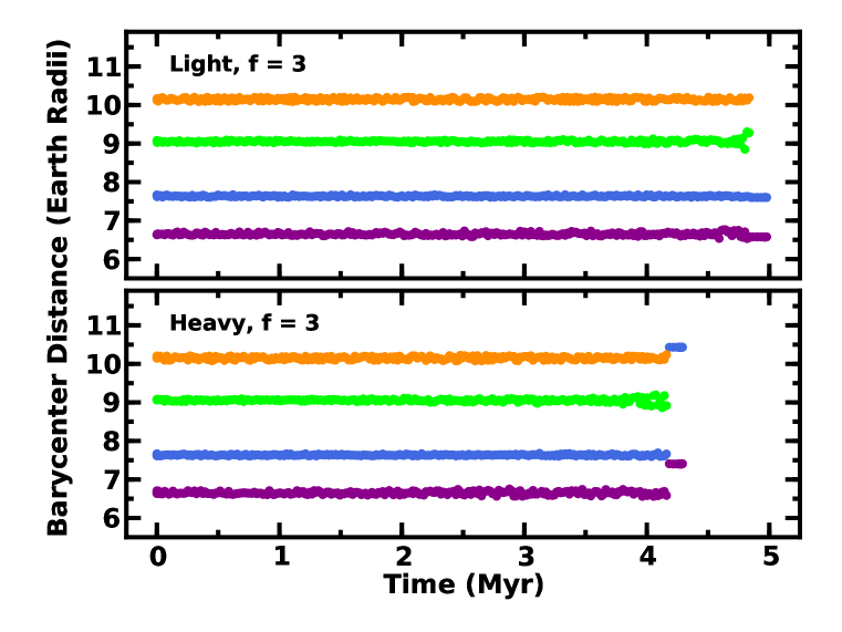
Figure 1: Satellite ejection in light (upper panel) and heavy (lower panel) systems with $N$ = 40 and mass ratio $f$ = 3 for all satellites. Symbols plot $r$ the distance from the barycenter for Styx (purple), Nix (blue), Kerberos (green), and Hydra (orange) as a function of time.

Fig. 1 illustrates the long-term evolution of systems where $f$ = 3 for all satellites. In the heavy system (lower panel), the satellites maintain a constant distance from the system barycenter for roughly 4 Myr. All of the satellites then develop eccentric orbits ($e$ = 0.06–0.2). Once Kerberos crosses the orbit of Hydra, both are lost. The remaining satellites lie on eccentric orbits at larger distances from the system barycenter.

In the light system, Nix and Hydra gradually excite the orbit of Kerberos. However, Kerberos is not massive enough to modify the orbits of Nix or Hydra. After nearly 5 Myr, Kerberos crosses the orbit of Hydra, destabilizing the orbits of both satellites. Both are ejected from the system. Although ejection has limited impact on $e$ for Styx and Nix, both orbit at somewhat smaller distances from the system barycenter.

Throughout the evolution, the oscillations in the orbital distances and eccentricities for satellites in the heavy system are larger than those in the light system. With a more massive Styx and Kerberos, the mutual gravitational interactions are larger in the heavy system, resulting in larger perturbations of the orbits. Despite this difference, lifetimes are not significantly different, 4.17 Myr for the heavy system and 4.85 Myr for the light system. Among all of the calculations for $f$ = 3, the heavy system has a marginally smaller median lifetime (2.9 Myr) than the light system (3 Myr). These lifetimes are much shorter than the 4.5 Gyr age of the solar system; thus, these systems are unlikely proxies for the Pluto-Charon satellite system.

Fig. 2 focuses on the last stages of a calculation with heavy satellites and $f_{H}$ = 1.8. Near the end of the evolution, the orbital distance of Kerberos (light green points) varies chaotically from roughly 8.5 $R_{\oplus}$ to nearly 9.5 $R_{\oplus}$ from the system barycenter. Because Styx (blue points) and Nix (dark green points) are much closer to Pluto-Charon than Kerberos, they are less affected by the large mass of Hydra (orange points). Near the end of the tracks, Kerberos crosses the path of Hydra, passing outside of Hydra’s orbit and pulling Hydra closer to Pluto-Charon. After reaching an orbital distance of 12 $R_{\oplus}$ from the barycenter, Kerberos returns to approach Hydra’s orbit and is then ejected. Hydra returns close to its original orbital distance, but on an eccentric orbit ($e$ = 0.05). Nix and Styx then lie on slightly wider, more eccentric orbits. The high eccentricity of Styx ($e$ = 0.14) guarantees that it will eventually cross the orbit of Nix and be ejected.

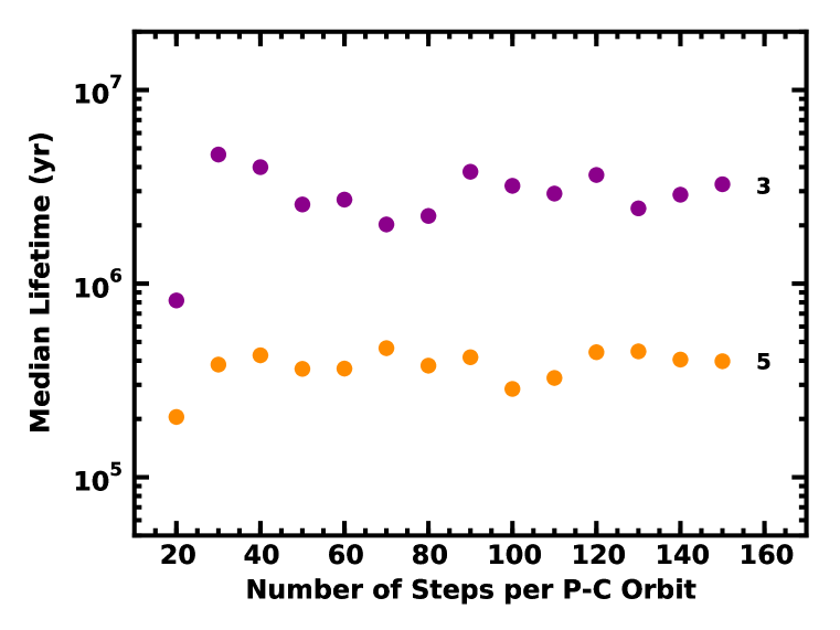
Figure 3: Median lifetime $\tau_{m}$ as a function of $N$ from 14–20 calculations of satellite systems with $f=$ 3 (purple symbols) and $f=$ 5 (orange symbols). Calculations with 30 or more steps per orbit yield similar values for $\tau_{m}$; simulations with $N$ = 20 result in much smaller lifetimes.

Fig. 3 shows results for the median lifetime of the satellite system for $N$ = 20–150, $f$ = 3, and $f$ = 5. For each combination of $N$ and $f$, 11–15 calculations yields a robust median; within the 1$\sigma$ dispersion of the lifetimes, the median and average lifetimes are identical. For $N$ = 30–150 and all $f$, the median lifetime is independent of $N$. When $N$ = 20, the average and median lifetimes are systematically smaller than calculations with larger $N$. This pattern persists for larger $f$, albeit with somewhat larger scatter.

4.4 Stability Considerations

In some calculations, none of the four small satellites are ejected after 900–1100 Myr of orbital integration. Completing 4.5 Gyr of integration is computationally intensive and beyond the scope of our effort. To judge whether these configurations are stable on 4.5 Gyr time scales, we perform statistical analyses of satellite orbits in each calculation.

To analyze the 20,000–100,000 snapshots for a simulation with no ejection, we compute the average distance $r_{avg,i}$ of each satellite from the barycenter and the average height $z_{avg,i}$ of each satellite from the plane of the Pluto-Charon binary for all snapshots; we then calculate $\delta r_{i}$ = $|r_{i}-r_{avg_{i}}|$ and $\delta z_{i}$ = $|z_{i}-z_{avg_{i}}|$. From estimates of the linear correlation coefficient (Pearson’s $r$), the Spearman rank-order correlation coefficient, and Kendall’s $\tau$ (Press et al., 1992), we test for trends in $\delta r_{i}$ and $\delta z_{i}$ with time. We then compute the standard deviation of $\delta r_{i}$ ($\sigma_{r,i}$) and $\delta z_{i}$ ($\sigma_{z,i}$). As a second test, we divide the snapshots into groups of 100, derive $r_{avg,i}$, $\delta r_{i}$, and $\sigma_{r,i}$ (and the corresponding $z$ variables) within each group, and search for trends of these variables from the first group of 100 snapshots to the last group of 100 snapshots.

Relative to a system where the four small satellites have zero mass, we consider whether an apparently stable light system has a large $\sigma_{r,i}$ ($\sigma_{z,i}$) or a significant trend of $\delta r_{i}$ ($\delta z_{i}$) with time. In a stable system, the typical dispersion in $\delta r_{i}$ is small, ranging from 0.01 $R_{\oplus}$ for Nix to 0.02 $R_{\oplus}$ for Hydra. There is no measurable trend of $\delta r_{i}$ with time: the three correlation coefficients are indistinguishable from zero at a high confidence level (probabilities $p>0.3$). The dispersions in $\delta z_{i}$ are a factor of 2–4 smaller than those in $\delta r_{i}$, with similarly small evidence of a trend with time, $p>0.5$. The lack of trends in the eccentricities (as measured by $\delta r_{i}$) or the inclinations (as measured by $\delta z_{i}$) with time suggest the orbits are stable.

In very unstable systems, the dispersion in $\delta r_{i}$ for Styx and Kerberos is somewhat larger and the three correlation coefficients are positive with probabilities $p<10^{-10}$ that the coefficients are consistent with zero. Often, there are also clear trends in $\delta z_{i}$ with time for Styx and Kerberos, with equally low probabilities that the correlation coefficients are consistent with zero.

There are a few systems where the trends in $\delta r_{i}$ and $\delta z_{i}$ with time are less obvious. Here, we rely on the Pearson, Spearman, and Kendall tests. When all probabilities from these tests are small, $p<10^{-3}$, the trend with time is significant at the 3-$\sigma$ (or better) level. We judge a system unstable. Longer-term integrations would likely yield more significant trends in $\delta r_{i}$ with time for these systems. When $10^{-2}>p>10^{-3}$, trends of $\delta r_{i}$ or $\delta z_{i}$ with time are not significant. These systems are marginally stable.

4.5 Main Results

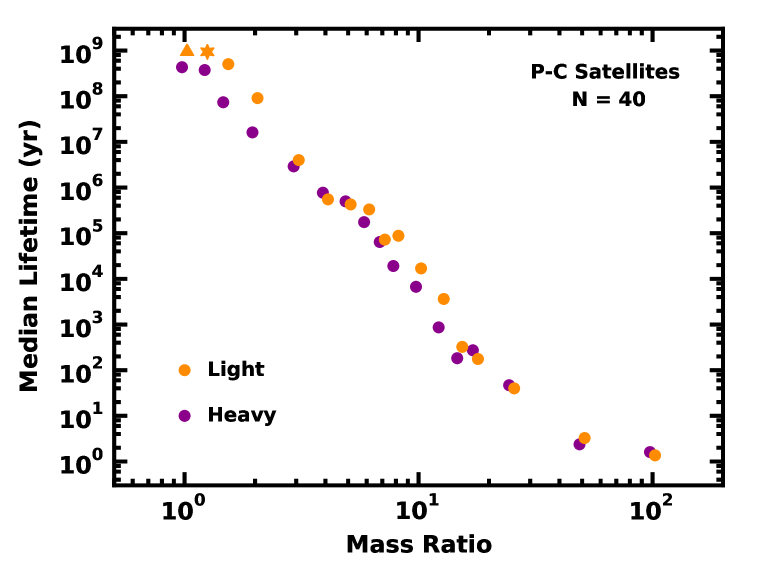
Figure 4: Median lifetime $\tau$ as a function of mass ratio $f$ for light (orange symbols) and heavy (purple symbols) satellite systems. Calculations yield lower limits on $\tau$ for marginally unstable light systems with $f$ = 1.0 (orange triangle) and clear unstable light systems with $f$ = 1.25 (orange hexagon).

In calculations where we multiply the masses of the small satellites by the same factor, $f$, the lifetime is very sensitive to the total mass (Fig. 4). Among the 7–10 calculations of systems with $f$ = 50 or $f$ = 100, at least one satellite is ejected within 1–3 yr. As we decrease $f$, there is a clear progression in the median lifetime $\tau_{m}$, from 10–100 yr for $f$ = 15–25 to 10 Myr for $f$ = 2. Among the calculations with $f\approx$ 1, lifetimes are 0.1–1 Gyr.

Heavy systems with $f\geq$ 1 are unstable. For each $f\geq$ 1.25, all simulations eject at least one satellite. Among the 14 simulations of heavy systems with $f$ = 1, eleven produce an ejection on time scales ranging from 70 Myr to 960 Myr. In two systems with no ejections, the orbital $e$ of Styx and Kerberos grows steadily with time. Only one of the 14 calculations maintains a nearly steady $e$ for Styx and Kerberos. Thus, there is a formal 93% likelihood that a heavy satellite system with $f$ = 1 is unstable on time scales at least a factor of five smaller than the age of the solar system.

Light systems with $f>1$ are also unstable. At large $f\geq$ 3, outcomes are chaotic; there is little difference in the lifetimes of light and heavy systems. When $f\leq$ 2, lifetimes for light satellite systems are 2–4 times longer than lifetimes for heavy systems. Among the configurations with $f\approx$ 1, none produce an ejection after nearly 1 Gyr of dynamical evolution. A few, however, show evidence for a slowly increasing $e$ in Styx or Kerberos or both. Thus, light systems with $f\approx$ 1 are marginally unstable. on 1 Gyr time scales

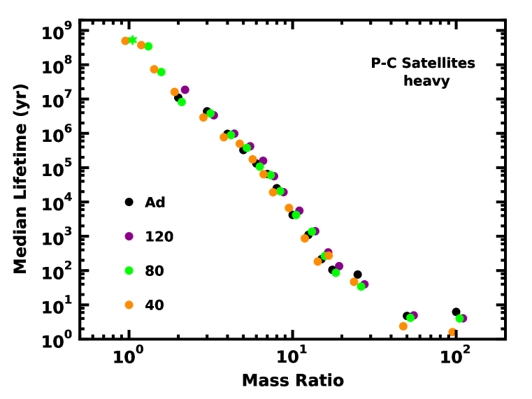
Figure 5: Median lifetime $\tau$ for heavy satellite systems as a function of mass ratio $f$ for four different integration routines as listed in the legend. Calculations with $N$ = 80 yield lower limits on $\tau$ for systems with the nominal masses, $f$ = 1 (starred symbols). Orbits of systems with initial masses $f$ times larger than the nominal satellite masses become unstable on time scales ranging from 1–10 yr ($f$ = 50–100) to $10^{7}-10^{8}$ yr ($f$ = 1.5–2).

These results are independent of the integrator (Fig. 5). For heavy systems with $f$ = 2–100, calculations with $N$ = 40, 80, and 120 yield the same $\tau_{m}$. The extra time spent to resolve close encounters with the adaptive integrator also has little impact on $\tau_{m}$ for $f$ = 2–100. When $f<$ 2, symplectic integrations with $N\geq$ 100 or adaptive integrations are too computationally intensive. However, symplectic integrations with $N$ = 80 yield the same median lifetimes for $f$ = 1 and $f$ = 1.5 as those with $N$ = 40.

Results for light systems are similar. For these calculations, we added an additional comparison with $N$ = 150. As with the heavy systems, the median lifetimes for $f\geq$ 2 are independent of the method of integration. For $f$ = 1.25 and 1.5, symplectic integrations with $N$ = 80 yield similar $\tau_{m}$ as those with $N$ = 40.

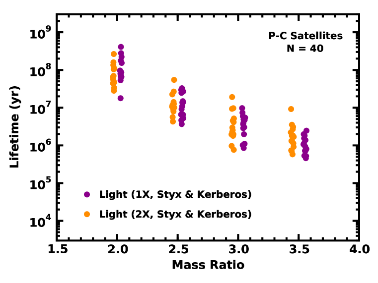
Figure 6: Comparison of lifetimes $\tau$ for the complete ensemble of calculations with $f$ = 2–3.5 for light satellite systems with the nominal masses for all satellites (purple symbols) and with double the nominal masses for Styx and Kerberos (orange symbols).

To check the sensitivity to input parameters in more detail, we consider calculations where Styx and Kerberos have twice their nominal masses in a light satellite system (Fig. 6). Results for $f$ = 2.5–3.5 show similar lifetimes for the two different masses of Styx and Kerberos. When $f$ = 2, the median lifetime for a light system with more massive Styx and Kerberos, $\tau\approx$ 60 Myr, is shorter than the median, $\tau\approx$ 90 Myr, for a light system with the nominal masses for Styx and Kerberos. Both median lifetimes are much shorter than the 4.5 Gyr age of the solar system. However, a KS test returns a probability of 15% that the two sets of lifetimes are drawn from the same parent distribution. Thus, the distributions of lifetimes are formally indistinguishable.

These results confirm the expectations of dynamical theory. Heavy systems with $f\geq$ 1 are unstable on time scales much shorter than the age of the solar system. Although they are more stable than heavy systems, light systems with $f\geq$ 1.25 are also unstable on relatively short time scales. Light systems with $f\approx$ 1 are marginally unstable on a 1 Gyr time scale. Although we have not completed calculations for light systems with twice the nominal mass of Styx and Kerberos and $f\leq$ 1.5, results for $f$ = 2–3.5 suggest the lifetimes are fairly independent of the masses of Styx and Kerberos.

To conclude this section, we examine sets of simulations where we augment the mass of one satellite ($f_{i}>$ 1 for $i$ either N, K, or H) and keep the masses of the other satellites at their nominal HST masses. We keep the mass of Styx fixed; its small mass precludes much improvement with $n$-body models. Instead of performing multiple calculations with very similar $f_{i}$, we derive lifetimes $\tau$ for calculations that densely sample $f_{i}=$ 1–6.

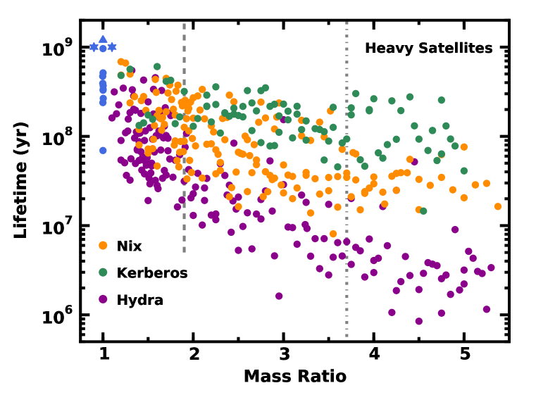
Figure 7: Lifetimes for heavy satellite systems with $f_{i}>1$ for Nix (orange points), Kerberos (green points), or Hydra (purple points) and $f$ = 1 for the other satellites. Several points have been displaced horizontally or vertically by small amounts for clarity. The vertical dashed (dotted) lines indicate 1$\sigma$ (3$\sigma$) upper limits on the masses from fits to HST data. Among the 14 distinct calculations with $f$ = 1 for all satellites (blue symbols), eleven resulted in at least one ejected satellite (filled circles), two are unstable with slowly growing $e$ for Styx and Kerberos but no ejection (filled hexagons), and one appears stable with an oscillating $e$ for Styx and Kerberos (filled triangle).

The results confirm that heavy satellite systems are unstable (Fig. 7). Models with $f_{H}$ = 1–1.4 have $\tau\approx$ 50–600 Myr. Although several calculations with larger mass ratios have similarly long lifetimes, $\tau$ declines monotonically with $f_{H}$, reaching $\tau\approx$ a few Myr for $f_{H}$ = 4–5. Calculations with a more massive Nix show a shallower variation of lifetime with $f_{N}$, ranging from $\tau\approx$ 20–40 Myr for $f_{N}\approx$ 4–5 to 60–700 Myr for $f_{N}\approx$ 1–1.6. Following this trend, the system lifetime has an even shallower dependence on the mass of Kerberos, with $\tau\approx$ 50–600 Myr for $f_{K}$ = 1–5.

In all of these simulations, systems where the mass of one satellite is larger than the nominal masses have much longer lifetimes than systems where all of the satellites are more massive. As an example, heavy systems with $f$ = 4–5 for all satellites have median lifetimes $\tau_{m}\sim$ 1 Myr. Systems with $f_{H}$ = 4–5 are somewhat more stable, with lifetimes of 1–10 Myr. When $f_{N}$ = 4–5, lifetimes are much longer, 10–100 Myr. Calculations with $f_{K}$ = 4–5 are even more stable, with lifetimes of 50–300 Myr.

This behavior correlates with the nominal masses of the three satellites. As the outermost and most massive satellite, Hydra has a significant impact on the dynamical evolution of the inner satellites. Making Hydra more massive tends to push the inner satellites towards the Pluto–Charon binary. As Pluto–Charon pushes back, the satellite system becomes unstable. In contrast, a more massive Nix or Kerberos tends to push Hydra away from the inner binary. With less pushback from Pluto–Charon, the more massive satellite system can then occupy a somewhat larger volume than the nominal system and have a somewhat longer lifetime.

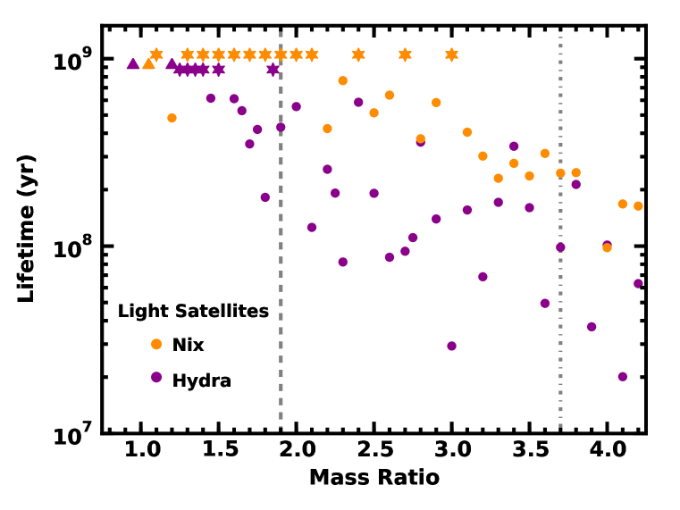
Figure 8: Lifetime $\tau$ for light satellite systems where the mass of Nix (orange symbols) or Hydra (purple symbols) has been augmented by a factor $f$ = 1–5. Hexagons (triangles) indicate lower limits on the lifetime for unstable (possibly stable) systems. Some points have been displaced vertically by 0.1 in the log for clarity. Gray vertical dashed (dot-dashed) lines mark 1$\sigma$ (3$\sigma$) limits on masses from HST data. Light systems with $f_{N}\geq$ 1.1 or $f_{H}\geq$ 1.15 are unstable.

Repeating this exercise with the light satellite system leads to similar conclusions (Fig. 8). Compared to the heavy system, light systems with $f_{H}$ = 3–4 survive $\sim$ ten times longer before ejecting either Styx or Kerberos. For $f_{H}$ = 3–4, the typical lifetime is 20–200 Myr. Systems with smaller $f_{H}$ have significantly longer lifetimes, with $\tau\approx$ 100–500 Myr at $f_{H}$ = 2 and $\tau\geq$ 400 Myr at $f_{H}\leq$ 1.75. Among the calculations with $f_{H}\leq$ 1.75, several produce an ejected satellite. In others, the orbital $e$ of Styx and Kerberos steadily increase in time. Although a light system with $f_{H}$ = 1.2 shows few signs of instability after 975 Myr of dynamical evolution, another system with $f_{H}$ = 1.1 is clearly unstable.

Systems with $f_{N}>1$ generally last much longer than those with $f_{H}>1$. Typical lifetimes range from $\sim$ 100 Myr at $f_{N}$ = 4 to $\sim$ 400 Myr at $f_{N}$ = 2.5–3.5 to more than 1 Gyr at $f_{N}$ = 1. Curiously, all of the calculations with $f_{N}\geq$ 1.1 show a steadily increasing $e$ with time for Styx and Kerberos. On times scales of 1–2 Gyr, we expect each of these calculations will result in an ejection of Styx or Kerberos.

4.6 Summary: Robust Satellite Masses

The $n$-body calculations suggest that the heavy (light) satellite system with the nominal masses is clearly (probably) unstable. Calculations for the light satellite system place the strongest constraints on the masses of Nix and Hydra. After $\sim$ 1 Gyr for many of 14 orbital integrations, the light system with $f$ = 1 occupies an unstable state where the $e$ of Styx and Kerberos gradually increase with time. Systems with $f\geq$ 1.25 eject at least one small satellite on time scales ranging from 1–10 yr ($f$ = 50–100) to $10^{4}$ yr ($f$ = 10) to 100–300 Myr ($f$ = 1.25–1.50).

Calculations where we vary the masses of Hydra or Nix independently of the other satellites yield robust upper limits for stable light systems: $f_{H}\leq$ 1.15 (when $f_{N}$ = 1) and $f_{N}<$ 1.1 (when $f_{H}$ = 1). Adopting $f\approx f_{N}\approx f_{H}$ implies an upper limit $f\leq$ 1.05 for stability. Despite the smaller number of these calculations, this upper limit agrees reasonably well with the limit $f\leq$ 1 derived from calculations of light systems with the nominal masses.

These calculations follows a long tradition of using stability to constrain the masses and orbital elements of known circumstellar and circumbinary planet and satellite systems (e.g., Duncan & Lissauer, 1997; Ito & Miyama, 2001; Fabrycky & Murray-Clay, 2010; French & Showalter, 2012; Youdin et al., 2012; Mahajan & Wu, 2014; Obertas et al., 2017, and references therein). In many of these studies, stability is inferred from fits to a set of direct $n$-body calculations (e.g., Duncan & Lissauer, 1997; French & Showalter, 2012; Youdin et al., 2012). The $n$-body results in these examples yield a relation between the lifetime of the system $t$ and the mass factor $f$,

$$t=t_{0}f^{-\beta}~{}.$$ (3)

When the processor time required to calculate stability for some range of $f$ is prohibitive, results for large $f$ are extrapolated to small $f$.

Our calculations provide a way to test this approach for the Pluto–Charon system. Fits to the full ensemble of calculations for $f$ = 2–100 yield $t_{0}$ and $\beta$. For the heavy satellite system, we may then compare the predicted $t$ at $f$ = 1 with the time scales inferred directly. For the light system, the $n$-body calculations provide good evidence for instability on time scales of $\sim$ 2 Gyr. Comparing this time scale with the predicted $t$ places stronger constraints on satellite masses.

To perform these fits, we employ the robust estimation routine MEDFIT (Press et al., 1992), which fits a straight line to a set of points by minimizing the absolute deviation. Converting Eq. 3 to a linear equation, fits to the data for the heavy system for $N$ = 40 and $f$ = 1–100 result in $t_{0}$ = 550 Myr and $\beta\approx$ 4.9. Considering the range $f$ = 2–100 yields very similar fits for $N$ = 40, 80, and 120 and for the adaptive integrator, $t_{0}$ = 300–600 Myr and $\beta$ = 4.8. Contracting the range in $f$ to 3–100 or 4–100 has little impact: $t_{0}$ = 600–700 Myr and $\beta$ = 5 for $f$ = 3 and $t_{0}$ = 500–700 Myr and $\beta$ = 4.9 for $f$ = 4. In all of these fits, the absolute deviation of the points from the fit is 0.3–0.4. Analyzing only those results with $f$ = 5–100 or $f$ = 6–100, however, degrades the quality of the fit; the absolute deviation and range in $t_{0}$ are then much larger.

For comparison, Youdin et al. (2012) derive $t_{0}\geq$ 200 Myr and $\beta$ = 3.6–4.6 for calculations of Pluto–Charon, Hydra, Kerberos, and Nix with $f\geq$ 4–10. From the full suite of $n$-body calculations described here, the median lifetime of a heavy system with $f$ = 1 is 430 Myr with a full range of 70 Myr to 960 Myr. Fits to results for $f$ = 2–100 capture this range rather well, predicting an average $t_{0}$ = 510 Myr. Adopting the absolute deviation as a measure of the full range of $t$ at any $f$ suggests a minimum $t\approx$ 250 Myr and a maximum $t\approx$ 1000 Myr, close to the range derived from the $n$-body calculations.

Repeating this analysis for the $n$-body calculations where we multiply the mass of only one satellite by a factor $f>1$ yields similar results. Fits to the $n$-body data for a heavy satellite system with $f_{H}\geq$ 1.5 yield $t_{0}$ = 300 Myr and $\beta$ = 3. Similar data for $f_{N}\geq$ 1.5 ($f_{K}\geq$ 1.5) generate $t_{0}$ = 375 Myr and $\beta$ = 1.75 ($t_{0}$ = 410 Myr and $\beta$ = 0.925). Taken together, the $t_{0}$ implied by this suite of $n$-body calculations for the heavy system agrees with the $t_{0}$ derived from those with a common $f$ for all satellites.

For the light system, the fit to the full ensemble of results for $N$ = 40 and $f$ = 1–100 returns $t_{0}\approx$ 2400 Myr and $\beta\approx$ 5.3. Removing data for $f<$ 2 allows a comparison for calculations with different $N$ and with the adaptive integrator: $t_{0}$ = 1500–2200 Myr and $\beta$ = 5.1–5.3. There is also little difference among the various fits for $f$ = 3–100, $f$ = 4–100, and $f$ = 5–100; all of the integrators suggest $t_{0}$ = 1000–3000 Myr and $\beta$ = 5.0–5.3. Removing more data from the analysis leads to a much larger range in $t_{0}$ and $\beta$ and generally larger absolute deviations. Although we cannot make a direct comparison between the lifetimes derived from $n$-body calculations and these fits, the growth in $e$ and $\imath$ of light systems with $f$ = 1 suggests lifetimes $\sim$ 2000 Myr. The two analyses clearly agree.

Among the $n$-body calculations for light systems with $f_{H}\neq 1$ or $f_{N}\neq 1$, only the data for $f_{H}\neq 1$ cover a sufficiently large range in $f$ to perform a high quality fit. With $t_{0}$ = 1600 Myr and $\beta$ = 2.6, the lifetime derived for these simulations is identical to the 2000 Myr lifetime implied by calculations with the same $f$ for all satellites.

Overall, this examination demonstrates a set of robust upper limits for the masses of Hydra and Nix. From the fits to the $n$-body simulations with identical $f$ for all satellites, light systems with $f$ = 0.75, 0.85, and 1.0 have median lifetimes of 10 Gyr, 4.5 Gyr, and 2 Gyr. Based on the factor of 2–3 dispersion in lifetimes among any calculation with fixed $f$, we expect survival rates of $\sim$ 0% ($f$ = 1.05-1.10), 10%–20% ($f$ = 1.0), 50% ($f$ = 0.85), or 90%–100% ($f$ = 0.75) for the 4.5 Gyr age of the solar system. Thus, reasonable upper limits to the masses of Nix and Hydra are $\sim$ 10% larger than their nominal masses. Among the calculations with $f_{H}>1$ or $f_{N}>$ 1, systems with $f_{H}$ somewhat larger than 1 are more stable than those with $f_{N}$ somewhat larger than 1. We therefore set the upper limits $f_{N}\leq$ 1.05 and $f_{H}\leq$ 1.15; together, these correspond well with $f\leq$ 1.1.

The $n$-body calculations in this study place weaker limits on the masses of Styx and Kerberos. Requiring at least one heavy system survive for 4.5 Gyr implies $t$ = 1500 Myr, $f\leq$ 0.8, and a total mass for the four satellites $\sim 9.1\times 10^{19}$ g. This mass is comparable to the mass of a light system with $f\approx$ 1, $\sim 9.3\times 10^{19}$ g. Thus, the $n$-body results for the heavy systems are consistent with the small mass for Kerberos and Styx adopted for the light systems. Once we complete calculations for light systems with $f$ = 1.5 and 2 and twice the nominal masses for Styx and Kerberos, it should be possible to place better limits on the masses of Styx and Kerberos.

5 SATELLITE MASS DENSITY

To estimate the mass density of Nix and Hydra, we consider the volume $V$ within three types of solids: boxes, ellipsoids, and pyramids. Defining $a$, $b$, $c$ as the lengths of the semiaxes with $a>b>c$, $V$ = $8abc$ (box), $4\pi abc/3$ (ellipsoid), or $8abc/3$ (pyramid). Of these options, approximating the satellites as boxes (pyramids) yields the largest (smallest) volume and the smallest (largest) mass density. As a plausible compromise, we derive the mass density from the volume of an ellipsoid. We infer $\rho_{N}\leq$ 1.57 g cm^-3 as the mass density for Nix ($f_{N}\leq$ 1.05) and $\rho_{H}\leq$ 1.44 g cm^-3 for Hydra ($f_{H}\leq$ 1.15).

If all satellites have the same mass density, we can estimate $\rho$ from the total mass, $m\lesssim 10^{19}$ g, established in the $n$-body and the total volume from the New Horizons size measurements in Table 1. The result, $\rho\lesssim$ 1.3 $\rm g~{}cm^{-3}$, is somewhat smaller than the upper limits on the mass density soley from Nix and Hydra.

Although these mass densities are smaller than the mass density for Charon, they do not include the uncertainties in the measured sizes. Rather than estimate a plausible range in an upper limit for the mass density from the errors in sizes, we estimate the probability of a particular mass density from a Monte Carlo calculation. The calculation assigns random sizes

$$x_{i}=x_{i,0}+f_{g}\delta x_{i}~{},$$ (4)

to each satellite, where $x$ is either $a$, $b$, or $c$, $i$ is N (for Nix) or H (for Hydra), and $f_{g}$ is a gaussian deviate from a random number generator. The subscript ‘0’ refers to the measured length of the semiaxis. With $a$, $b$, and $c$ known, the volume $V_{i}$ for a box, ellipsoid or pyramid follows.

To choose the mass, we consider three approaches. In the simplest estimate, we adopt the upper limit derived from the $n$-body calculations,

$$m_{i}=m_{u,i},$$ (5)

where $m_{u,i}$ is 5% (15%) larger than the nominal mass for Nix (Hydra). As a second approach, we consider the nominal mass $m_{i,0}$ and adopted error $\delta m_{i}$ from the $n$-body calculations, deriving a model mass

$$m_{i}=m_{i,0}+f_{g}\delta m_{i}~{}.$$ (6)

The mass density is then $\rho_{i}=m_{i}/V_{i}$. Finally , we adopt a lower limit to the mass $m_{i,l}$ and set the mass as

$$m_{i}=m_{l,i}+f(m_{u,i}-m_{l,i})~{},$$ (7)

where $f$ is a uniform deviate between 0 and 1. Repeating each procedure $N$ times yields three probability distributions for $\rho_{i}$.

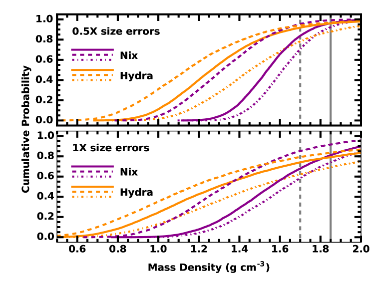
Figure 9: Cumulative probability that Nix (purple curves) and Hydra (orange curves) have a density smaller than $\rho$ using mass model 1 (dot-dashed curves), mass model 2 (solid curves), or mass model 3 (dashed curves) for the Monte Carlo calculations described in the text. Lower panel: volume derived from the nominal errors. Upper panel: volume derived from errors half the size of the nominal errors. Vertical dashed (solid) grey lines indicate the measured mass density of Charon (Pluto). For plausible masses of Nix and Hydra, their mass density is most likely smaller than the mass density of Charon and significantly smaller than the mass density of Pluto.

Fig. 9 and Table 3 summarize the results. The cumulative probability distributions $p(\rho<\rho)$ have several characteristic features. Due to the smaller errors in its size, Nix has sharper distributions for all mass models; $p(\rho)$ for Hydra is much broader. Given the smaller volume of Nix relative to Hydra, the probability that Nix has a mass density smaller than the mass density of Charon is smaller than the corresponding probability for Hydra for any mass model. At larger mass densities, this behavior reverses: for two of three mass models, Nix has a higher probability of having mass density smaller than the mass density of Pluto.

These results suggest that the mass densities of Nix and Hydra are smaller than those of Charon and Pluto. In the most conservative mass model 1, roughly 59% (62%) of the Monte Carlo trials yield a mass density for Nix (Hydra) smaller than that of Charon (see Table 3). In the most liberal model 3, these probabilities grow to $\sim$ 80%. From our calculations, the most likely masses for Nix and Hydra are close to their nominal masses (e.g., model 2). In this picture, Nix and Hydra have mass densities smaller than Charon $\sim$ 70% of the time.

The Monte Carlo calculations demonstrate that reducing errors in the size estimates for Nix and Hydra place much better constraints on the mass density. For the nominal sizes, reducing the errors by a factor of two improves the likelihood of mass densities smaller than Charon by as much as 15% to 20%. Stronger limits on the masses generate weaker improvements of the probabilities.

Reducing the uncertainties in the satellite shapes would also enable better estimates for the mass density. From published New Horizons images, Nix does not resemble a pyramid and looks more like an ellipsoid than a box. Deriving a 3D shape from the full ensemble of New Horizons images would eliminate this ambiguity. For Hydra, the poorer image resolution complicates volume estimates. As with Nix, using the complete set of imaging data would considerably reduce uncertainties in the volume.

6 DISCUSSION

The new limits on the masses for the Pluto–Charon satellites allow us to (i) compare their properties with other satellites in the solar system, (ii) improve our understanding of the stability of circumbinary planetary/satellite systems, and (iii) examine how the satellites find their places after the giant impact that formed the central binary. Before summarizing our overall conclusions, we briefly consider each of these topics.

6.1 Comparison with Other Satellite Systems

Starting with Mars (Phobos and Deimos) and continuing outward from the Sun with Jupiter (Carme, Metis, and Sinope), Saturn (Atlas, Daphnis, Helen, and Pan), Uranus (Cordelia and Ophelia), and Neptune (Laomedeia, Psamanthe, and Sao), satellites with radii of 5–20 km are common throughout the solar system (e.g., Thomas, 1989; Thomas et al., 1998; Karkoschka, 2001; Rettig et al., 2001; Karkoschka, 2003; Thomas, 2010; Sheppard et al., 2006; Slyuta, 2014). Imaging data from Voyager, Cassini, New Horizons, and various missions to Mars reveal a variety of shapes and structures on the surfaces of these small satellites.

Despite extensive knowledge about their surface characteristics, measurements of the mass density for small satellites (radii less than 50–100 km) are rare. The densities of Phobos (1.9 $\rm g~{}cm^{-3}$) and Deimos (1.5 $\rm g~{}cm^{-3}$) are much larger than those of the somewhat larger Prometheus (0.5 $\rm g~{}cm^{-3}$) and Pandora (0.5 g cm^-3; Jacobson & French, 2004; Renner et al., 2005; Jacobson, 2010; Pätzold et al., 2014). The density of Uranus’ moon Cressida (0.9 $\rm g~{}cm^{-3}$) is roughly midway between the two Martian satellite and Saturn’s satellites orbiting close to or within the ring system (Chancia et al., 2017). Estimates for the densities of other small satellites rely on estimates instead of direct measurement of their masses.

Mass density estimates for Nix and Hydra place them within the broad range of measured densities of satellites with similar sizes. Their densities are clearly smaller than the density of Phobos and probably comparable to the density of Deimos. Due to the lack of other satellites in the system, the factor of three reduction in mass required to have mass densities comparable to Daphnis, Prometheus, Pandora, and the other ring moons of Saturn seems unlikely (Kenyon & Bromley, 2019). Discovery of other small satellites with orbits between Styx and Hydra would test this assertion.

Pluto’s small satellites distinguish themselves with their large albedos, ranging from 0.56 for Styx and Kerberos to 0.83 for Hydra (Weaver et al., 2016). Despite their similar mass density, albedos of Phobos and Deimos, $\approx$ 0.07, are roughly an order of magnitude smaller than the albedos of Styx, Nix, Kerberos, and Hydra (Zellner & Capen, 1974; Thomas et al., 1996; Cantor et al., 1999). Aside from Triton (0.72; Hicks & Buratti, 2004), all of the satellites of Uranus and Neptune have albedos smaller than 0.4 (e.g., Karkoschka, 2001, 2003; Fry & Sromovsky, 2007; Farkas-Takács et al., 2017, and references therein). Among Jupiter’s satellites, only Io, Europa, and Ganymede have albedos larger than 0.4 (Buratti & Veverka, 1983; Simonelli & Veverka, 1984). In contrast, many of Saturn’s satellites have albedos comparable to those of Pluto’s small satellites (Verbiscer et al., 2007; Pitman et al., 2010). Among the smaller satellites, Helene and Calypso have albedos of order unity (see also Madden & Kaltenegger, 2018, and references therein).

The similarity of the Pluto–Charon and the small, inner satellites of Saturn could be a result of similar formation mechanisms. In the Saturn system, the origin of the rings remains controversial (e.g., Charnoz et al., 2009; Canup, 2010; Hyodo et al., 2017; Dubinski, 2019, and references therein). However, small moons outside and within Saturn’s rings likely grew from ring material and either migrated outside the rings (e.g., Charnoz et al., 2010) or generated gaps within the rings (e.g., Bromley & Kenyon, 2013, and references therein). The density of the moons and moonlets within the rings is then similar to the low density of ring material. In the Pluto–Charon system, the satellites form within the icy debris of a giant impact, which has a lower density than Pluto or Charon, but probably has a larger density than the material in Saturn’s rings.

6.2 Circumbinary Dynamics

As discussed in §3, there have been numerous studies into the stability of multi-planet (multi-satellite) systems orbiting single stars (planets) (e.g., Wisdom, 1980; Petit & Henon, 1986; Gladman, 1993; Chambers et al., 1996; Deck et al., 2013; Fang & Margot, 2013; Kratter & Shannon, 2014; Fabrycky et al., 2014; Mahajan & Wu, 2014; Pu & Wu, 2015; Morrison & Kratter, 2016; Obertas et al., 2017; Hwang et al., 2017; Quarles & Lissauer, 2018). With two objects, stability requires a minimum separation in Hill units, $K=2\sqrt{3}$, that is independent of planet masses and orbital periods. In multi-planet systems, orbital resonances complicate stability arguments. Although systems with three or more planets may be stable with $K\approx$ 6–7, systems with larger separations, $K\approx$ 10–12, are more generally stable for the age of a solar-type star.

With few studies of the stability circumbinary multi-planet systems (e.g., Kratter & Shannon, 2014; Marzari & Gallina, 2016), results for the Pluto–Charon system enhance our understanding of the circumbinary dynamics of multi-planet systems. In our calculations, the heavy system with the nominal masses has $K_{SN}$ = 12, $K_{NK}$ = 16, and $K_{KH}$ = 10; this system is clearly unstable on 500 Myr time scales. Fits to the full quite of simulations for heavy systems suggests a roughly 50% survival rate on time scales of 10 Gyr for $f\approx$ 0.5, which is equivalent to a system with $K_{SN}$ = 15, $K_{NK}$ = 20, and $K_{KH}$ = 12.5.

Among light satellite systems, a 50% survival rate over 10 Gyr requires $f\approx$ 0.75. Satellite separations in Hill units are then nearly identical to the separations of stable heavy systems, $K_{SN}$ = 14.5, $K_{NK}$ = 19, and $K_{KH}$ = 12. Generalizing to any satellite system around Pluto–Charon is challenging due to the orbital resonances (Smullen & Kratter, 2017), but it seems that this set of orbital separations would allow stability for other masses of the Pluto–Charon satellites.

6.3 Formation Models

The Pluto-Charon satellite system provides a fascinating challenge to planet formation theories. Current ideas focus on the aftermath of a giant impact, where a glancing collision between Pluto and Charon leads to an eccentric binary system with a period of 1–2 d (McKinnon, 1989; Canup, 2005, 2011). Satellites grow in circumbinary debris from the collision or in material captured afterwards (Stern et al., 2006; Lithwick & Wu, 2008a; Canup, 2011; Pires dos Santos et al., 2012; Kenyon & Bromley, 2014; Walsh & Levison, 2015).

This basic picture faces several hurdles. On a time scale of 1–10 Myr, tidal forces circularize and expand the Pluto-Charon orbit (Farinella et al., 1979; Dobrovolskis et al., 1997; Peale et al., 2011; Cheng et al., 2014a). As the central binary evolves, orbital resonances pass through the volume containing the debris (Ward & Canup, 2006; Lithwick & Wu, 2008b; Smullen & Kratter, 2017). These resonances pump the eccentricities of circumbinary solids, destabilizing systems of satellites with properties similar to those of the known satellites (Peale et al., 2011; Cheng et al., 2014b; Walsh & Levison, 2015; Bromley & Kenyon, 2015b; Smullen & Kratter, 2017; Woo & Lee, 2018). Although satellites embedded within rings of small particles survive resonance pumping, the ensemble of small particles must be massive enough to damp the orbits of larger satellites (Bromley & Kenyon, 2015b).

The time scale to grow satellites out of the debris is comparable to the circularization time (Kenyon & Bromley, 2014; Walsh & Levison, 2015). In systems where the expansion of the binary is complete, the number, masses, and orbital architecture of the satellites depend on the initial mass of the debris: more massive rings of debris favor fewer large satellites, while less massive rings favor many small satellites. Numerical simulations match the current number of satellites with an initial mass of $3-10\times 10^{19}$ g for the debris (Kenyon & Bromley, 2014). The upper end of this range is consistent with the upper limit on satellite mass derived here. The Kenyon & Bromley (2014) simulations also predict several much smaller satellites with radii $R\leq$ 1–3 km beyond the orbit of Hydra. Although new satellites have not been identified (Weaver et al., 2016), a significant discovery space is accessible with the James Webb Space Telescope and other NASA missions (Kenyon & Bromley, 2019; Gaslac Gallardo et al., 2019).

Other aspects of the New Horizons data support this general model for satellite formation. In a giant impact where Charon survives, the circumbinary debris should have a larger proportion of ice than either Pluto or Charon. The densities derived for Nix and Hydra agree with this prediction. The large measured albedos for all of the satellites also imply an icier mixture than inferred for Pluto or Charon (Weaver et al., 2016). Finally, the shapes of the satellites also look like the products of an agglomeration process (Weaver et al., 2016).

The close packing of the satellites orbiting Pluto-Charon – with orbital separations of $K=12-18$ in units of mutual Hill radii – is reminiscent of several exoplanetary systems discovered by the Kepler satellite – including Kepler 11, Kepler 80, Kepler 90, Kepler 223, and K2-138 – where $n_{p}\geq$ 4–5 planets orbit near resonances and have close to the minimum orbital separation necessary for stability (Borucki et al., 2011; Lissauer et al., 2011; Mahajan & Wu, 2014; Mills et al., 2016; MacDonald et al., 2016; Shallue & Vanderburg, 2018; Granados Contreras & Boley, 2018; Christiansen et al., 2018). Tightly packed orbits appear to be a natural outcome of planet formation; it is tempting to conclude that the Pluto-Charon satellites formed in a similar process.

In current theory, systems of planets orbiting close to resonances result from radial migration (Lee & Peale, 2002; Mustill & Wyatt, 2011; Pierens & Nelson, 2013; Pierens et al., 2013; Zhang et al., 2014; MacDonald et al., 2016; Mills et al., 2016; Luger et al., 2017; Tamayo et al., 2017; Ormel et al., 2017). As protoplanets grow within a circumstellar gaseous disk, torques from the disk cause the planet to migrate radially inward or outward through the disk at a rate that depends on the mass of the planet and the physical properties of the disk. When pairs of migrating protoplanets enter an orbital resonance, the energy required to leave the resonance is often larger than the energy available from migration. Pairs of planets may then remain ‘stuck’ in the resonance or migrate together at rates that maintain the resonance. This process can repeat for systems of planets, yielding ‘migration chains’ where sequential pairs of planets are at or in orbital resonance.

Applying this idea to the Pluto-Charon system requires some simple modifications. Instead of a gaseous disk around a fairly stable, single or binary central star, newly-formed satellites migrate through a disk of small particles surrounding an expanding binary. For the observed satellite masses, typical migration rates in circumbinary disks are large enough to generate resonant chains of satellites (Kenyon & Bromley, 2014). If the lifetime of the circumbinary disk is longer than the expansion time for the central binary, collisional damping between the small particles and the satellites is strong enough to maintain the resonances (Bromley & Kenyon, 2015b). Once the expansion of the binary is complete, the satellites can disperse the disk of small particles, leaving the satellites close to orbital resonance as observed.

Using numerical simulations to test the plausibility of this picture requires accurate masses for the four small satellites. The total mass of the satellite system derived here, $\lesssim 10^{20}$ g, provides a new target for theoretical models that attempt to predict the growth of satellites within circumbinary debris from the Pluto-Charon collision (Kenyon & Bromley, 2014; Walsh & Levison, 2015) or the long-term stability of satellites as the binary circularizes and expands following the collision (Bromley & Kenyon, 2015b; Cheng et al., 2014b; Smullen & Kratter, 2017; Woo & Lee, 2018). The smaller masses for the satellites may also improve our understanding of their rotational evolution (Quillen et al., 2017).

7 SUMMARY

To generate robust constraints on the masses of the four small satellites in the Pluto–Charon system, we perform a large set of $n$-body calculations. The results yield clear upper limits for the masses of Nix and Hydra, $\sim$ 10% larger than the nominal masses derived from HST observations. Best estimates are $m_{N}\lesssim 4.7\times 10^{19}$ g and $m_{H}\lesssim 5.5\times 10^{19}$ g. The estimate for Nix agrees with previous limits derived from $n$-body simulations (Youdin et al., 2012). Results for Hydra are $\sim$ 50% lower than limits derived in Youdin et al. (2012).

The calculations also demonstrate that the mass of Kerberos is much smaller than inferred from orbital fits to HST imaging data; $m_{K}\approx 10^{18}$ g is consistent with the $n$-body calculations. Limits on the mass of Styx are much weaker; however, a plausible estimate consistent with the numerical calculations is $m_{S}\approx 6\times 10^{17}$.

Together with large albedos derived from New Horizons, upper limits on the masses of Nix and Hydra suggest they formed in an icier mixture than Charon or Pluto. Using size measurements from New Horizons, the mass densities are $\rho_{N}\lesssim$ 1.57 $\rm g~{}cm^{-3}$ for Nix and $\rho_{H}\lesssim$ 1.44 $\rm g~{}cm^{-3}$ for Hydra. A numerical analysis that includes uncertainties in the measured sizes implies a 70% (80%) probability that the mass densities of Nix and Hydra are smaller than the mass density of Charon (Pluto).

These results provide new insight into the formation and evolution of circumbinary planet and satellite systems. For Pluto–Charon, stability of the four small satellites on 5–10 Gyr time scales requires satellite separations, $K=\delta a_{ij}/R_{H,ij}\geq$ 12, where $\delta a_{ij}$ is the absolute value of the difference in semimajor axes between adjacent satellites and $R_{H,ij}$ is their mutual Hill radius. The ensemble of satellite masses implies formation in a moderate mass ring of material (e.g., Kenyon & Bromley, 2014).

Improving constraints on the mass density of Nix and Hydra requires better models for their shapes and volumes. Together with new $n$-body calculations, frequency mapping, perturbation, and variational methods can upgrade mass estimates for Styx and Kerberos. Even without these advances, the new satellite masses allow better tests of models for the formation and long-term stability of circumbinary planets and satellites.

Resources supporting this work on the ‘discover’ cluster were provided by the NASA High-End Computing (HEC) Program through the NASA Center for Climate Simulation (NCCS) at Goddard Space Flight Center. We thank M. Geller, K. Kratter, M. Payne, and A. Youdin for advice, comments, and encouragement. Portions of this project were supported by the NASA Outer Planets and Emerging Worlds programs through grants NNX11AM37G and NNX17AE24G.

Binary output files from the simulations, C programs capable of reading the binary files, and some ASCII text files derived from the simulations are available at a publicly accessible repository (https://hive.utah.edu/) with digital object identifier TBD.

Table 1: Nominal satellite properties for $n$-body calculations

Satellite	$m_{i}$	$r_{i}$ (km)	$\rho_{i}$ ($\rm g~{}cm^{-3}$)	$r_{H}$ (km)	$a_{i}$ (km)	$e$ ($\times 10^{-3}$)	$\imath$ (deg)	$P_{orb}$ (d)
Styx (heavy)	4.5	5.2	6.46	198	42656	5.787	0.809	20.16155
Styx (light)	0.6	5.2	1.02	101	42656	5.787	0.809	20.16155
Nix	45.0	19.3	1.49	487	48694	2.036	0.133	24.85463
Kerberos (heavy)	16.5	6.0	18.2	405	57783	3.280	0.389	32.16756
Kerberos (light)	1.0	6.0	1.11	160	57783	3.280	0.389	32.16756
Hydra	48.0	20.9	1.26	661	64738	5.862	0.242	38.20177

Table 2: Starting conditions for $n$-body calculations

Satellite	$x$ (km)	$y$ (km)	$z$ (km)	$v_{x}$ (km s-1)	$v_{y}$ (km s-1)	$v_{z}$ (km s-1)
Pluto-0	-157.9402301682	-456.9060813269	-2071.3208302900	-0.0177029949	-0.0158012994	0.0048365588
Pluto-1	-157.8310490659	-456.8246643552	-2071.4634491000	-0.0177033115	-0.0158016253	0.0048363507
Pluto-2	-157.8121679944	-456.7988459683	-2071.4067337364	-0.0177032091	-0.0158015359	0.0048362971
Charon	1297.1743847853	3752.6022617472	17011.9058384535	0.1453959509	0.1297771902	-0.0397230040
Styx	-30572.8427772584	-26535.8134344897	12311.2908958766	0.0232883189	0.0427977975	0.1464990284
Nix	9024.3487802378	15210.7370165008	45591.7573572213	0.1004334400	0.0865524814	-0.0479498746
Kerberos	23564.2070250521	28380.0399507624	44578.0258218278	0.0792537026	0.0630220100	-0.0817084451
Hydra	-43331.3261132443	-43628.4575945387	-20506.5419357332	-0.0374001038	-0.0184905611	0.1157937283

Table 3: Monte Carlo Statistics for Mass Density of Nix and Hydra

Modela	$\rho_{N,med}$	$p(\rho_{N}<\rho_{C})$	$p(\rho_{N}<\rho_{P})$	$\rho_{H,med}$	$p(\rho_{H}<\rho_{C})$	$p(\rho_{H}<\rho_{P})$
1a	1.63	0.59	0.75	1.49	0.62	0.70
2a	1.55	0.68	0.81	1.29	0.74	0.79
3a	1.33	0.85	0.92	1.17	0.79	0.84
1b	1.61	0.70	0.92	1.46	0.78	0.88
2b	1.54	0.84	0.96	1.26	0.92	0.96
3b	1.32	0.95	0.99	1.14	0.94	0.97

Figure 2: As in Fig. 1 for a system with $N$ = 40 and a massive Hydra ($f_{H}$ = 1.8) in a heavy system with nominal masses for the other satellites.

References

- Batygin & Brown (2016) Batygin, K., & Brown, M. E. 2016, AJ, 151, 22
- Becker et al. (2018) Becker, J. C., Khain, T., Hamilton, S. J., et al. 2018, AJ, 156, 81
- Borucki et al. (2011) Borucki, W. J., Koch, D. G., Basri, G., et al. 2011, ApJ, 736, 19
- Brasser et al. (2016) Brasser, R., Matsumura, S., Ida, S., Mojzsis, S. J., & Werner, S. C. 2016, ApJ, 821, 75
- Bromley & Kenyon (2006) Bromley, B. C., & Kenyon, S. J. 2006, AJ, 131, 2737
- Bromley & Kenyon (2011a) —. 2011a, ApJ, 731, 101
- Bromley & Kenyon (2011b) —. 2011b, ApJ, 735, 29
- Bromley & Kenyon (2013) —. 2013, ApJ, 764, 192
- Bromley & Kenyon (2014) —. 2014, ApJ, 796, 141
- Bromley & Kenyon (2015a) —. 2015a, ApJ, 806, 98
- Bromley & Kenyon (2015b) —. 2015b, ApJ, 809, 88
- Bromley & Kenyon (2016) —. 2016, ApJ, 826, 64
- Bromley & Kenyon (2017) —. 2017, AJ, 153, 216
- Brown & Batygin (2016) Brown, M. E., & Batygin, K. 2016, ApJ, 824, L23
- Brown & Batygin (2019) —. 2019, AJ, 157, 62
- Brozović et al. (2015) Brozović, M., Showalter, M. R., Jacobson, R. A., & Buie, M. W. 2015, Icarus, 246, 317
- Buie et al. (2013) Buie, M. W., Grundy, W. M., & Tholen, D. J. 2013, AJ, 146, 152
- Buie et al. (2006) Buie, M. W., Grundy, W. M., Young, E. F., Young, L. A., & Stern, S. A. 2006, AJ, 132, 290
- Buie et al. (2012) Buie, M. W., Tholen, D. J., & Grundy, W. M. 2012, AJ, 144, 15
- Buie et al. (1997) Buie, M. W., Tholen, D. J., & Wasserman, L. H. 1997, Icarus, 125, 233
- Buratti & Veverka (1983) Buratti, B., & Veverka, J. 1983, Icarus, 55, 93
- Burns et al. (1979) Burns, J. A., Lamy, P. L., & Soter, S. 1979, Icarus, 40, 1
- Cantor et al. (1999) Cantor, B. A., Wolff, M. J., Thomas, P. C., James, P. B., & Jensen, G. 1999, Icarus, 142, 414
- Canup (2005) Canup, R. M. 2005, Science, 307, 546
- Canup (2010) —. 2010, Nature, 468, 943
- Canup (2011) —. 2011, AJ, 141, 35
- Chambers et al. (1996) Chambers, J. E., Wetherill, G. W., & Boss, A. P. 1996, Icarus, 119, 261
- Chancia et al. (2017) Chancia, R. O., Hedman, M. M., & French, R. G. 2017, AJ, 154, 153
- Charnoz et al. (2009) Charnoz, S., Morbidelli, A., Dones, L., & Salmon, J. 2009, Icarus, 199, 413
- Charnoz et al. (2010) Charnoz, S., Salmon, J., & Crida, A. 2010, Nature, 465, 752
- Chavez et al. (2015) Chavez, C. E., Georgakarakos, N., Prodan, S., et al. 2015, MNRAS, 446, 1283
- Cheng et al. (2014a) Cheng, W. H., Lee, M. H., & Peale, S. J. 2014a, Icarus, 233, 242
- Cheng et al. (2014b) Cheng, W. H., Peale, S. J., & Lee, M. H. 2014b, Icarus, 241, 180
- Christiansen et al. (2018) Christiansen, J. L., Crossfield, I. J. M., Barentsen, G., et al. 2018, AJ, 155, 57
- Christy & Harrington (1978) Christy, J. W., & Harrington, R. S. 1978, AJ, 83, 1005
- Clement et al. (2019) Clement, M. S., Kaib, N. A., Raymond, S. N., Chambers, J. E., & Walsh, K. J. 2019, Icarus, 321, 778
- Dawson & Murray-Clay (2012) Dawson, R. I., & Murray-Clay, R. 2012, ApJ, 750, 43
- Deck et al. (2013) Deck, K. M., Payne, M., & Holman, M. J. 2013, ApJ, 774, 129
- Dobrovolskis et al. (1997) Dobrovolskis, A. R., Peale, S. J., & Harris, A. W. 1997, in Pluto and Charon, ed. S. A. Stern & D. J. Tholen (University of Arizona Press, Tucson, AZ), 159–191
- Doolin & Blundell (2011) Doolin, S., & Blundell, K. M. 2011, MNRAS, 418, 2656
- Dubinski (2019) Dubinski, J. 2019, Icarus, 321, 291
- Duncan et al. (1998) Duncan, M. J., Levison, H. F., & Lee, M. H. 1998, AJ, 116, 2067
- Duncan & Lissauer (1997) Duncan, M. J., & Lissauer, J. J. 1997, Icarus, 125, 1
- Fabrycky & Murray-Clay (2010) Fabrycky, D. C., & Murray-Clay, R. A. 2010, ApJ, 710, 1408
- Fabrycky et al. (2014) Fabrycky, D. C., Lissauer, J. J., Ragozzine, D., et al. 2014, ApJ, 790, 146
- Fang & Margot (2013) Fang, J., & Margot, J.-L. 2013, ApJ, 767, 115
- Farinella et al. (1979) Farinella, P., Milani, A., Nobili, A. M., & Valsecchi, G. B. 1979, Moon and Planets, 20, 415
- Farkas-Takács et al. (2017) Farkas-Takács, A., Kiss, C., Pál, A., et al. 2017, AJ, 154, 119
- French & Showalter (2012) French, R. S., & Showalter, M. R. 2012, Icarus, 220, 911
- Fry & Sromovsky (2007) Fry, P. M., & Sromovsky, L. A. 2007, Icarus, 192, 117
- Gaslac Gallardo et al. (2019) Gaslac Gallardo, D. M., Giuliatti Winter, S. M., & Pires, P. 2019, MNRAS, 484, 4574
- Gladman (1993) Gladman, B. 1993, Icarus, 106, 247
- Gomes et al. (2004) Gomes, R. S., Morbidelli, A., & Levison, H. F. 2004, Icarus, 170, 492
- Granados Contreras & Boley (2018) Granados Contreras, A. P., & Boley, A. C. 2018, AJ, 155, 139
- Hamilton & Burns (1992) Hamilton, D. P., & Burns, J. A. 1992, Icarus, 96, 43
- Hicks & Buratti (2004) Hicks, M. D., & Buratti, B. J. 2004, Icarus, 171, 210
- Holman & Wiegert (1999) Holman, M. J., & Wiegert, P. A. 1999, AJ, 117, 621
- Holman et al. (2018) Holman, M. J., Payne, M. J., Fraser, W., et al. 2018, ApJ, 855, L6
- Hwang et al. (2017) Hwang, J. A., Steffen, J. H., Lombardi, Jr., J. C., & Rasio, F. A. 2017, MNRAS, 470, 4145
- Hyodo et al. (2017) Hyodo, R., Charnoz, S., Ohtsuki, K., & Genda, H. 2017, Icarus, 282, 195
- Ida et al. (2000) Ida, S., Bryden, G., Lin, D. N. C., & Tanaka, H. 2000, ApJ, 534, 428
- Ito & Miyama (2001) Ito, T., & Miyama, S. M. 2001, ApJ, 552, 372
- Izidoro et al. (2014) Izidoro, A., Haghighipour, N., Winter, O. C., & Tsuchida, M. 2014, ApJ, 782, 31
- Jacobson (2010) Jacobson, R. A. 2010, AJ, 139, 668
- Jacobson & French (2004) Jacobson, R. A., & French, R. G. 2004, Icarus, 172, 382
- Karkoschka (2001) Karkoschka, E. 2001, Icarus, 151, 69
- Karkoschka (2003) —. 2003, Icarus, 162, 400
- Kenyon & Bromley (2014) Kenyon, S. J., & Bromley, B. C. 2014, AJ, 147, 8
- Kenyon & Bromley (2019) —. 2019, AJ, 157, 79
- Kratter & Shannon (2014) Kratter, K. M., & Shannon, A. 2014, MNRAS, 437, 3727
- Lam & Kipping (2018) Lam, C., & Kipping, D. 2018, MNRAS, 476, 5692
- Lauer et al. (2018) Lauer, T. R., Throop, H. B., Showalter, M. R., et al. 2018, Icarus, 301, 155
- Lee & Peale (2002) Lee, M. H., & Peale, S. J. 2002, ApJ, 567, 596
- Lee & Peale (2006) —. 2006, Icarus, 184, 573
- Leung & Lee (2013) Leung, G. C. K., & Lee, M. H. 2013, ApJ, 763, 107
- Levison & Morbidelli (2003) Levison, H. F., & Morbidelli, A. 2003, Nature, 426, 419
- Li et al. (2016) Li, G., Holman, M. J., & Tao, M. 2016, ApJ, 831, 96
- Lissauer et al. (2011) Lissauer, J. J., Fabrycky, D. C., Ford, E. B., et al. 2011, Nature, 470, 53
- Lithwick & Wu (2008a) Lithwick, Y., & Wu, Y. 2008a, ArXiv e-prints, arXiv:0802.2951
- Lithwick & Wu (2008b) —. 2008b, ArXiv e-prints, arXiv:0802.2939
- Luger et al. (2017) Luger, R., Sestovic, M., Kruse, E., et al. 2017, Nature Astronomy, 1, 0129
- MacDonald et al. (2016) MacDonald, M. G., Ragozzine, D., Fabrycky, D. C., et al. 2016, AJ, 152, 105
- Madden & Kaltenegger (2018) Madden, J. H., & Kaltenegger, L. 2018, Astrobiology, 18, 1559
- Mahajan & Wu (2014) Mahajan, N., & Wu, Y. 2014, ApJ, 795, 32
- Malhotra (1993) Malhotra, R. 1993, Nature, 365, 819
- Marzari & Gallina (2016) Marzari, F., & Gallina, G. 2016, A&A, 594, A89
- McKinnon (1989) McKinnon, W. B. 1989, ApJ, 344, L41
- McKinnon et al. (2017) McKinnon, W. B., Stern, S. A., Weaver, H. A., et al. 2017, Icarus, 287, 2
- Michaely et al. (2017) Michaely, E., Perets, H. B., & Grishin, E. 2017, ApJ, 836, 27
- Mills et al. (2016) Mills, S. M., Fabrycky, D. C., Migaszewski, C., et al. 2016, Nature, 533, 509
- Morrison & Kratter (2016) Morrison, S. J., & Kratter, K. M. 2016, ApJ, 823, 118
- Mustill & Wyatt (2011) Mustill, A. J., & Wyatt, M. C. 2011, MNRAS, 413, 554
- Nagy et al. (2006) Nagy, I., Süli, Á., & Érdi, B. 2006, MNRAS, 370, L19
- Nimmo et al. (2017) Nimmo, F., Umurhan, O., Lisse, C. M., et al. 2017, Icarus, 287, 12
- Obertas et al. (2017) Obertas, A., Van Laerhoven, C., & Tamayo, D. 2017, Icarus, 293, 52
- Ormel et al. (2017) Ormel, C. W., Liu, B., & Schoonenberg, D. 2017, A&A, 604, A1
- Pätzold et al. (2014) Pätzold, M., Andert, T. P., Tyler, G. L., et al. 2014, Icarus, 229, 92
- Peale et al. (2011) Peale, S. J., Cheng, W. H., & Lee, M. H. 2011, in EPSC-DPS Joint Meeting 2011, 665
- Petit & Henon (1986) Petit, J., & Henon, M. 1986, Icarus, 66, 536
- Pierens et al. (2013) Pierens, A., Cossou, C., & Raymond, S. N. 2013, A&A, 558, A105
- Pierens & Nelson (2013) Pierens, A., & Nelson, R. P. 2013, A&A, 556, A134
- Pires Dos Santos et al. (2011) Pires Dos Santos, P. M., Giuliatti Winter, S. M., & Sfair, R. 2011, MNRAS, 410, 273
- Pires dos Santos et al. (2013) Pires dos Santos, P. M., Giuliatti Winter, S. M., Sfair, R., & Mourão, D. C. 2013, MNRAS, 430, 2761
- Pires dos Santos et al. (2012) Pires dos Santos, P. M., Morbidelli, A., & Nesvorný, D. 2012, Celestial Mechanics and Dynamical Astronomy, 114, 341
- Pitman et al. (2010) Pitman, K. M., Buratti, B. J., & Mosher, J. A. 2010, Icarus, 206, 537
- Poppe & Horányi (2011) Poppe, A., & Horányi, M. 2011, Planet. Space Sci., 59, 1647
- Porter & Stern (2015) Porter, S. B., & Stern, S. A. 2015, ArXiv e-prints, arXiv:1505.05933
- Press et al. (1992) Press, W. H., Teukolsky, S. A., Vetterling, W. T., & Flannery, B. P. 1992, Numerical recipes in FORTRAN. The art of scientific computing (Cambridge: University Press)
- Pu & Wu (2015) Pu, B., & Wu, Y. 2015, ApJ, 807, 44
- Quarles & Lissauer (2018) Quarles, B., & Lissauer, J. J. 2018, AJ, 155, 130
- Quarles et al. (2018) Quarles, B., Satyal, S., Kostov, V., Kaib, N., & Haghighipour, N. 2018, ApJ, 856, 150
- Quillen et al. (2017) Quillen, A. C., Nichols-Fleming, F., Chen, Y.-Y., & Noyelles, B. 2017, Icarus, 293, 94
- Renner et al. (2005) Renner, S., Sicardy, B., & French, R. G. 2005, Icarus, 174, 230
- Rettig et al. (2001) Rettig, T. W., Walsh, K., & Consolmagno, G. 2001, Icarus, 154, 313
- Saha & Tremaine (1992) Saha, P., & Tremaine, S. 1992, AJ, 104, 1633
- Shallue & Vanderburg (2018) Shallue, C. J., & Vanderburg, A. 2018, AJ, 155, 94
- Sheppard et al. (2018) Sheppard, S., Trujillo, C., Tholen, D., & Kaib, N. 2018, arXiv e-prints, arXiv:1810.00013
- Sheppard et al. (2006) Sheppard, S. S., Jewitt, D., & Kleyna, J. 2006, AJ, 132, 171
- Sheppard & Trujillo (2016) Sheppard, S. S., & Trujillo, C. 2016, AJ, 152, 221
- Showalter & Hamilton (2015) Showalter, M. R., & Hamilton, D. P. 2015, Nature, 522, 45
- Showalter et al. (2011) Showalter, M. R., Hamilton, D. P., Stern, S. A., et al. 2011, IAU Circ., 9221, 1
- Showalter et al. (2012) Showalter, M. R., Weaver, H. A., Stern, S. A., et al. 2012, IAU Circ., 9253, 1
- Simonelli & Veverka (1984) Simonelli, D. P., & Veverka, J. 1984, Icarus, 59, 406
- Slyuta (2014) Slyuta, E. N. 2014, Solar System Research, 48, 217
- Smith & Lissauer (2009) Smith, A. W., & Lissauer, J. J. 2009, Icarus, 201, 381
- Smullen & Kratter (2017) Smullen, R. A., & Kratter, K. M. 2017, MNRAS, 466, 4480
- Smullen et al. (2016) Smullen, R. A., Kratter, K. M., & Shannon, A. 2016, MNRAS, 461, 1288
- Stern et al. (2018) Stern, S. A., Grundy, W. M., McKinnon, W. B., Weaver, H. A., & Young, L. A. 2018, ARA&A, 56, 357
- Stern et al. (2006) Stern, S. A., Weaver, H. A., Steffl, A. J., et al. 2006, Nature, 439, 946
- Stern et al. (2015) Stern, S. A., Bagenal, F., Ennico, K., et al. 2015, Science, 350, aad1815
- Süli & Zsigmond (2009) Süli, Á., & Zsigmond, Z. 2009, MNRAS, 398, 2199
- Sutherland & Fabrycky (2016) Sutherland, A. P., & Fabrycky, D. C. 2016, ApJ, 818, 6
- Tamayo et al. (2017) Tamayo, D., Rein, H., Petrovich, C., & Murray, N. 2017, ApJ, 840, L19
- Tholen et al. (2008) Tholen, D. J., Buie, M. W., Grundy, W. M., & Elliott, G. T. 2008, AJ, 135, 777
- Thomas (1989) Thomas, P. C. 1989, Icarus, 77, 248
- Thomas (2010) —. 2010, Icarus, 208, 395
- Thomas et al. (1996) Thomas, P. C., Adinolfi, D., Helfenstein, P., Simonelli, D., & Veverka, J. 1996, Icarus, 123, 536
- Thomas et al. (1998) Thomas, P. C., Burns, J. A., Rossier, L., et al. 1998, Icarus, 135, 360
- Trujillo & Sheppard (2014) Trujillo, C. A., & Sheppard, S. S. 2014, Nature, 507, 471
- Tsiganis et al. (2005) Tsiganis, K., Gomes, R., Morbidelli, A., & Levison, H. F. 2005, Nature, 435, 459
- Verbiscer et al. (2007) Verbiscer, A., French, R., Showalter, M., & Helfenstein, P. 2007, Science, 315, 815
- Walsh & Levison (2015) Walsh, K. J., & Levison, H. F. 2015, AJ, 150, 11
- Walsh et al. (2011) Walsh, K. J., Morbidelli, A., Raymond, S. N., O’Brien, D. P., & Mandell, A. M. 2011, Nature, 475, 206
- Ward & Canup (2006) Ward, W. R., & Canup, R. M. 2006, Science, 313, 1107
- Weaver et al. (2006) Weaver, H. A., Stern, S. A., Mutchler, M. J., et al. 2006, Nature, 439, 943
- Weaver et al. (2016) Weaver, H. A., Buie, M. W., Buratti, B. J., et al. 2016, Science, 351, aae0030
- Wisdom (1980) Wisdom, J. 1980, AJ, 85, 1122
- Wisdom & Holman (1991) Wisdom, J., & Holman, M. 1991, AJ, 102, 1528
- Woo & Lee (2018) Woo, J. M. Y., & Lee, M. H. 2018, AJ, 155, 175
- Yoshida (1990) Yoshida, H. 1990, Physics Letters A, 150, 262
- Youdin et al. (2012) Youdin, A. N., Kratter, K. M., & Kenyon, S. J. 2012, ApJ, 755, 17
- Zellner & Capen (1974) Zellner, B. H., & Capen, R. C. 1974, Icarus, 23, 437
- Zhang et al. (2014) Zhang, X., Liu, B., Lin, D. N. C., & Li, H. 2014, ApJ, 797, 20