Potential model for nuclear astrophysical fusion reactions with a square-well potential

Abstract

The potential model for nuclear astrophysical reactions requires a considerably shallow nuclear potential when a square-well potential is employed to fit experimental data. We discuss the origin of this apparently different behavior from that obtained with a smooth Woods-Saxon potential, for which a deep potential is often employed. We argue that due to the sharp change of the potential at the boundary the radius parameter tends to be large in the square-well model, which results in a large absorption radius. The wave function then needs to be suppressed in the absorption region, which can eventually be achieved by using a shallow potential. We thus clarify the reason why the square-well potential has been able to reproduce a large amount of fusion data.

I Introduction

Heavy-ion fusion reactions, such as ¹²C+¹²C and ¹⁶O+¹⁶O reactions, play an important role in nuclear astrophysics BTW85 ; BD04 ; TN09 . These reactions take place at extremely low energies, and a direct measurement of the reaction cross sections to obtain the astrophysical fusion rates is almost impossible. It is therefore indispensable to extrapolate experimental data at higher energies down to the region which is relevant to nuclear astrophysics. For this purpose, the potential model with a Woods-Saxon potential has often been used. Alternatively, one can also use a square-well potential, as has been advocated very successfully by Michaud and Fowler MF70 . The fusion probability can be evaluated analytically with such a square-well potential, and the calculation becomes considerably simplified. See e.g., Refs. Tang12 ; Zhang16 for recent applications of the square-well model to the ¹²C+¹²C and ¹²C+¹³C reactions.

Despite its simple nature, a square-well potential accounts for a large amount of experimental data, sometimes even better than a fit with a Woods-Saxon potential BTW85 . However, it has been recognized that the resultant square-well potential, that is used for a total (the nuclear + the Coulomb) potential, has to be repulsive Fowler75 ; Dayras76 . For instance, for the ¹²C+¹²C reaction, the best fit was obtained with the square-well potential, $V(r)=V_{0}\,\theta(R-r)~{}~{}(r\leq R)$, with $V_{0}=+5.8$ MeV and $R=7.50$ fm Fowler75 . Even though the value of $V_{0}$ is somewhat smaller than the Coulomb energy at $r=R$, that is, $V_{c}=6.9$ MeV, and thus the nuclear interaction is still attractive, the potential depth for the nuclear potential, $V_{0}-V_{c}$, is only 1.1 MeV, which is unusually small. The same tendency has been also found for the ¹²C+¹⁶O and the ¹⁶O+¹⁶O reactions Fowler75 .

The purpose of this paper is to clarify the origin of a shallow depth of a square-well potential for nuclear astrophysical reactions. To this end, we shall study the sensitivity of fusion cross sections to the parameters of the square-well potential, such as the range of the imaginary part and the depth of the real part.

II Square-well potential model

In the square-well potential model, one considers the following radial wave function for the relative motion between two nuclei BTW85 :

$$u(r) = Te^{-iKr}~{}~{}~{}~{}~{}~{}~{}~{}~{}~{}~{}~{}~{}~{}~{}~{}~{}~{}~{}~{}~{}~{}~{}~{}(r<R),$$ (1)

$$= H_{l}^{(-)}(kr)-S_{l}H_{l}^{(+)}(kr)~{}~{}~{}~{}(r\geq R),$$ (2)

with $K=\sqrt{2\mu[E-(V_{0}-iW_{0})]/\hbar^{2}}$ and $k=\sqrt{2\mu E/\hbar^{2}}$, $\mu$ and $E$ being the reduced mass and the incident energy in the center of mass frame, respectively. Here, $T$ and $S_{l}$ are the transmission and reflection coefficients, respectively, and $l$ is the partial wave. $H_{l}^{(+)}$ and $H_{l}^{(-)}$ are the outgoing and the incoming Coulomb wave functions, respectively, which are given in terms of the regular and the irregular Coulomb wave functions as $H_{l}^{(\pm)}=G_{l}\pm F_{l}$. The form of the wave function for $r<R$ is nothing but the incoming wave boundary condition HT12 ; ccfull , which assumes a strong absorption in the region $r<R$. The imaginary part of the square well potential, $-iW_{0}$, allows an absorption even for $E<V_{0}$. From the matching condition of the wave function at $r=R$, one obtains MSV70

$$1-|S_{l}|^{2}=\frac{4\frac{P_{l}}{KR}}{\left(1+\frac{P_{l}}{KR}\right)^{2}+\left(\frac{s_{l}}{KR}\right)^{2}},$$ (3)

with

$$P_{l} = \frac{kR}{F_{l}^{2}+G_{l}^{2}},$$ (4)

$$s_{l} = kR\,\frac{F_{l}F_{l}^{\prime}+G_{l}G_{l}^{\prime}}{F_{l}^{2}+G_{l}^{2}},$$ (5)

where the right hand side of Eqs. (4) and (5) are evaluated at $kR$. Fusion cross sections are then computed as HT12 ,

$$\sigma_{\rm fus}(E)=\frac{\pi}{k^{2}}\,\sum_{l}(2l+1)(1-|S_{l}|^{2}).$$ (6)

With those fusion cross sections, the astrophysical $S$-factor is defined as,

$$S(E)=E\sigma_{\rm fus}(E)\,e^{2\pi\eta(E)},$$ (7)

where $\eta(E)=Z_{P}Z_{T}e^{2}/(\hbar v)$ is the Sommerferd parameter. Here, $Z_{P}$ and $Z_{T}$ are the charge number of the projectile and the target nuclei, respectively, and $v=\sqrt{2E/\mu}$ is the velocity for the relative motion.

For fusion of two identical bosons, such as ¹²C+¹²C and ¹⁶O+¹⁶O, one has to symmetrize the wave function with respect to the interchange of the two nuclei. The fusion cross sections are then evaluated as RH15 ,

$$\sigma_{\rm fus}(E)=\frac{\pi}{k^{2}}\,\sum_{l}(1+(-1)^{l})(2l+1)(1-|S_{l}|^{2}).$$ (8)

In this case, only even partial waves contribute to fusion cross sections.

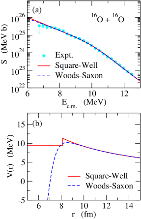
Figure 1: (The upper panel) The astrophysical $S$-factor for the ¹⁶O+¹⁶O reaction. The solid and the dashed lines are obtained with a square-well and a Woods-Saxon potentials, respectively. The experimental data are taken from Ref. Thomas86 . (The lower panel) The radial dependence of the total potentials used in the calculations shown in the upper panel.

The upper panel of Fig. 1 shows the astrophysical $S$-factor for the ¹⁶O+¹⁶O reaction. The solid line is obtained with a square-well potential with $V_{0}=9.4$ MeV, $R=8.13$ fm, and $W_{0}=2.1$ MeV. The reduced mass is taken to be $\mu=m(^{16}{\rm O})/2$, where $m(^{16}{\rm O})$ is the experimental mass for the ¹⁶O nucleus. For comparison, the figure also shows the result of the Woods-Saxon potential with the depth, the range, and the diffuseness parameters for the real part of $V_{0}=-54.5$ MeV, $R=6.5$ fm, and $a=0.45$ fm, respectively (the dashed line). The parameters for the imaginary part are taken to be $W_{0}=10.0$ MeV, $R_{w}=5$ fm, and $a_{w}=0.1$ fm. Those calculations are compared with the experimental data Thomas86 . One can see that both calculations reproduce the data equally well.

The lower panel of the figure shows the radial dependence of the two potentials employed. Evidently, the square-well potential is much shallower than the Woods-Saxon potential. One can also see that the range of the nuclear potential is much larger in the square-well potential as compared to the Woods-Saxon potential. We have confirmed that these features remain the same even if we replace $e^{-iKr}$ in Eq. (1) with $H_{l}^{(-)}(Kr)$ by taking into account the centrifugal and the Coulomb potentials in the inner region.

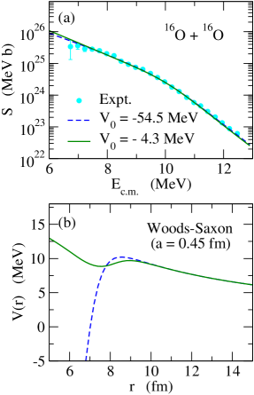
Figure 2: Same as Fig. 1, but with a shallow Woods-Saxon potential (the solid lines). The meaning of the dashed line is the same as in Fig. 1.

Because of continuous and discrete ambiguities of optical potentials BTW85 ; Hodgson1 ; Hodgson2 ; Cook80 , the parameters of the Woods-Saxon potential may not be determined uniquely. For instance, Fig. 2 shows the result with $V_{0}=-4.3$ MeV, $R=8.13$ fm, $a=0.45$ fm, $W_{0}=10$ MeV, $R_{w}=7.55$ fm, and $a_{w}=0.1$ fm. This potential is much shallower than the Woods-Saxon potential shown in Fig. 1, but still yields a comparable fit to the experimental data. That is, one can reproduce the data equally well by using either a deep potential with a small value of $R$ or a shallow potential with a larger value of $R$. Notice that the latter potential has a similar feature to the square-well potential shown in Fig. 1.

For a Woods-Saxon potential, a change in the radius parameter can be compensated with a change in the depth parameter so that the height of the Coulomb barrier remains the same. In contrast, for the square-well potential, the potential changes abruptly at $r=R$, and the height of the Coulomb barrier is determined only by $R$. That is, the height is independent of $V_{0}$. The value of $R$ then cannot be too small, otherwise the Coulomb barrier is too high, considerably suppressing the astrophysical $S$-factor at $E\gtrsim 10$ MeV.

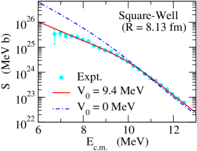
Figure 3: Comparison of the astrophysical $S$-factor for the ¹⁶O+¹⁶O system obtained with two different depth parameters of the square-well potential. The solid line is the same as that in Fig. 1 and is obtained with $V_{0}=9.4$ MeV, while the dot-dashed line is obtained with $V_{0}=0$ MeV. The range parameter of the square-well potential is set to be $R=8.13$ fm for both cases. The experimental data are taken from Ref. Thomas86 .

In the square-well model of Michaud and Fowler, the range parameters for the real and the imaginary parts are set to be the same to each other BTW85 ; MF70 ; Fowler75 . A large value of $R$ for the real part then implies that the flux is absorbed from relatively large distances. In order to see this, Fig. 3 shows the result of the square-well potential with $V_{0}=0$ MeV, for which the inner region is classically allowed for the entire range of energy shown in the figure. One can observe that this calculation overestimates the astrophysical $S$-factor at energies below 10 MeV. Notice that, when the potential is shallow, the wave function in the inner region is largely damped if the incident energy is below $V_{0}$. Evidently, one has to make the potential shallow in order to reproduce the experimental data, which results in a hindrance of the absorption effect.

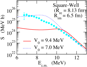
Figure 4: Same as Fig. 3, but for the case where the range parameter of the imaginary part of the square-well potential is set independently to that for the real part. Those are taken to be 8.13 fm and 6.5 fm for the real and the imaginary parts, respectively. The solid line is obtained with $V_{0}=9.4$ MeV, while the dotted line is obtained with $V_{0}=7.0$ MeV. The experimental data are taken from Ref. Thomas86 .

One would then expect that the depth of the square-well potential becomes deeper if the absorption range is shorter. This is indeed the case as is shown in Fig. 4, which is obtained by setting the range parameters for the real and the imaginary parts to be 8.13 and 6.5 fm, respectively. Notice that, in this case, the absorption does not start even if the relative motion penetrates through the barrier and reaches at $r=R$. To draw Fig. 4, we employ the boundary conditions of

$$u(r) = Te^{-iKr}~{}~{}~{}~{}~{}~{}~{}~{}~{}~{}~{}~{}~{}~{}~{}~{}~{}~{}~{}~{}~{}~{}~{}~{}(r<R_{i}),$$ (9)

$$= Ae^{-i\tilde{K}r}+Be^{i\tilde{K}r}~{}~{}~{}~{}~{}~{}~{}(R_{i}\leq r<R),$$ (10)

with $\tilde{K}=\sqrt{2\mu(E-V_{0})/\hbar^{2}}$. The boundary condition for the outer region, $r\geq R$, remains the same as in Eq. (2). The solid line in the figure is obtained with the same value of $V_{0}$ as in Fig. 3. Since the relative motion has further to penetrate the barrier before the absorption is effective, the astrophysical $S$-factor is largely underestimated. This is cured to some extent by deepening the potential depth, as is shown by the dotted line, which is obtained with $V_{0}=7.0$ MeV. The reproduction of the experimental data, however, is less satisfactory as compared to the solid line in Fig. 3. If the depth of the potential is further deepened, the astrophysical $S$-factors are overestimated as in the dot-dashed line in Fig. 3. Therefore, the choice of $R_{i}\neq R$ for the square-well model does not seem to be preferred, at least for the ¹⁶O+¹⁶O system.

III Summary

We have investigated the origin of a shallow depth of a square-well potential for nuclear astrophysical reactions. We have argued that this is caused by the following two effects. Firstly, the square-well potential changes abruptly at the boundary, leading to a large radius parameter. Because of this, the absorption of the flux starts from relatively large distances. The potential depth then becomes shallow in order to hinder the absorption effect. It is important to notice that these are artifacts of a square-well potential, and a shallow depth has nothing to do with microscopic origins of a repulsive core in internuclear potentials, such as the Pauli principle effect Tamagaki65 ; Baye82 . Indeed, if one uses a Woods-Saxon potential, one can employ a more reasonable value for the radius and the depth parameters. This would imply that a care must be taken in interpreting the results of a square-well model and in extrapolating the results down to astrophysically relevant energies, even though the model is simple and convenient, and often provides a good fit to experimental data.

References

- (1) C.A. Barnes, S. Trentalange, and S.-C. Wu, Treatise on Heavy-Ion Science, edited by D.A. Bromley (Plenum Press, New York, 1985), Vol. 6, p. 1.
- (2) C.A. Bertulani and P. Danielewicz, Introduction to Nuclear Reactions (IOP Publishing, Bristol, UK, 2004).
- (3) I.J. Thompson and F.M. Nunes, Nuclear Reactions for Astrophysics (Cambridge University Press, Cambridge, 2009).
- (4) G. Michaud and W.A. Fowler, Phys. Rev. C2, 2041 (1970).
- (5) X.D. Tang et al., J. of Phys. Conf. Ser. 337, 012016 (2012).
- (6) N.T. Zhang et al., EPJ Web of Conf. 109, 09003 (2016).
- (7) W.A. Fowler, G.R. Caughlan, and B.A. Zimmerman, Ann. Rev. Astron. and Astrophysics 13, 69 (1975).
- (8) R.A. Dayras, R.G. Stokstad, Z.E. Switkowski, and R.M. Wieland, Nucl. Phys. A265, 153 (1976).
- (9) K. Hagino and N. Takigawa, Prog. Theo. Phys. 128, 1061 (2012).
- (10) K. Hagino, N. Rowley, and A.T. Kruppa, Comput. Phys. Comm. 123, 143 (1999).
- (11) G. Michaud, L. Scherk, and E. Vogt, Phys. Rev. C1, 864 (1970).
- (12) N. Rowley and K. Hagino, Phys. Rev. C91, 044617 (2015).
- (13) J. Thomas et al., Phys. Rev. C33, 1679 (1986).
- (14) P.E. Hodgson, Nuclear Reactions and Nuclear Structure (Oxford University Press, London, 1971).
- (15) P.E. Hodgson, Nuclear Heavy-Ion Reactions (Oxford University Press, Oxford, 1978).
- (16) J. Cook, J.M. Barnwell, N.M. Clarke, and R.J. Griffiths, J. of Phys. G6, 1251 (1980).
- (17) R. Tamagaki and H. Tanaka, Prog. Theo. Phys. 34, 191 (1965).
- (18) D. Baye and N. Pecher, Nucl. Phys. A379, 330 (1982).