On the scaling behaviour of the alternating spin chain

Abstract

In this note we report the results of our study of a 1D integrable spin chain whose critical behaviour is governed by a CFT possessing a continuous spectrum of scaling dimensions. It is argued that the computation of the density of Bethe states of the continuous theory can be reduced to the calculation of the connection coefficients for a certain class of differential equations whose monodromy properties are similar to those of the conventional confluent hypergeometric equation. The finite size corrections to the scaling are also discussed.

Going back to Kadanoff’s block spin transformation, the concept of the Renormalization Group (RG) is usually illustrated by means of a finite statistical lattice system that provides a regularization of the Euclidean path integral. Within the Hamiltonian picture, attempts to introduce the scale transformation for a finite lattice system meet immediate difficulties. Of course, since the Hilbert space is not isomorphic for different lattice sizes, the scale transformation only makes sense for the low energy part of the spectrum. It is clear how to assign the size dependence for the ground state or, for that matter, the lowest energy states in the disjoint sectors of the Hilbert space. However forming individual RG flows trajectories for low energy stationary states that are densely distributed does not seem to be a trivial task. One dimensional quantum spin chains provide an ideal laboratory for studying this problem.

In the case of a critical spin chain subject to (quasi) periodic boundary conditions, conformal invariance predicts a so-called tower structure Cardy:1986ie for the excitation energy $\Delta E$ over the ground state for the low-energy part of the spectrum:

$$\Delta E=\frac{2\pi v_{\rm F}}{L}\ \big{(}d_{s}+{N}+\bar{N}\big{)}+o(L^{-1})\ .$$ (1)

Here $d_{s}$ are the scaling dimensions of the conformal primary; $N$, $\bar{N}$ are non-negative integers describing the excitations; and $v_{\rm F}$ is the Fermi velocity. In many cases the finite size corrections, denoted by $o(L^{-1})$, turn out to be small even for a lattice size $L$ that is not too large. Thus, despite the large degeneracies, the tower structure is often useful for identifying the scaling behaviour of the stationary states on the finite lattice provided that the spectrum of the scaling dimensions $\{d_{s}\}$ is discreet. In the presence of a continuous component in the set $\{d_{s}\}$, the practical use of eq. (1) becomes problematic.

Critical spin chain systems exhibiting a continuous spectrum of scaling dimensions are of considerable interest in many aspects, including the quantization of 2D non-linear sigma models on non-compact spaces and their applications to the description of condensed matter systems with disorder. In the work Jacobsen:2005xz the remarkable observation was made that the critical behaviour of the alternating spin chain originally introduced in Baxter:1971 ; Baxter is described by a CFT possessing a continuous spectrum of scaling dimensions. The model turns out to be an integrable system, which makes a detailed study of its RG flow possible. This was the subject of the papers Ikhlef:2008zz ; Ikhlef:2011ay ; Frahm:2012eb ; Candu:2013fva ; Frahm:2013cma , where some important results were obtained. In this note we present a summary of our study of the RG flow in the alternating spin chain. A detailed analysis and derivations will be given elsewhere.

The subject of our interest is a spin-$\frac{1}{2}$ chain of length $2L$ governed by the Hamiltonian

$${\mathbb{H}} = \frac{1}{\sin(2\gamma)}\ \sum_{m=1}^{2L}\,\Big{(}\,2\sin^{2}(\gamma)\,\sigma^{z}_{m}\,\sigma^{z}_{m+1}-(\sigma^{x}_{m}\,\sigma^{x}_{m+2}+\sigma^{y}_{m}\,\sigma^{y}_{m+2}+\sigma^{z}_{m}\,\sigma^{z}_{m+2})$$

$$+ {\rm i}\,(-1)^{m}\sin(\gamma)(\sigma^{x}_{m}\,\sigma^{y}_{m+1}-\sigma^{y}_{m}\,\sigma^{x}_{m+1})(\sigma^{z}_{m-1}-\sigma^{z}_{m+2})\,\Big{)}+2L\,\cot(2\gamma)\ .$$

In order to lift degeneracies in the energy spectrum as much as possible, instead of the periodic spin chain we will consider quasi periodic boundary conditions

$$\sigma^{\pm}_{2L+m}=\mbox{e}^{\pm 2{\rm i}\pi{\tt k}}\ \sigma^{\pm}_{m}\ ,\ \ \ \ \ \ \ \sigma^{z}_{2L+m}=\sigma^{z}_{m}\ \ \ \ \ \ \ \ \ \big{(}\sigma^{\pm}\equiv\textstyle\frac{1}{2}\,(\sigma^{x}\pm{\rm i}\,\sigma^{y})\,\big{)}\ ,$$ (3)

involving the parameter ${\tt k}$ lying within the “first Brillouin zone”

$$-\textstyle\frac{1}{2}<{\tt k}\leq\textstyle\frac{1}{2}\ .$$

The Hamiltonian (On the scaling behaviour of the alternating spin chain) is connected to an alternating 6-vertex model. Its $R$-matrix, $R_{12}(\beta)$, is an operator depending on the spectral parameter $\beta$ and acting in the product of two vector spaces ${\mathbb{C}}^{2}\otimes{\mathbb{C}}^{2}$. We denote its matrix elements as $R_{12}(\beta)_{a_{1}a_{2}}^{b_{1}b_{2}}$, where the indices take two values $\pm 1$. The indices $a_{1},b_{1}$ and $a_{2},b_{2}$ refer to the first and second spaces, respectively. There are only six non-zero matrix elements of $R_{12}(\beta)$, which are given by

$$R_{12}(\beta)^{++}_{++}= R_{12}(\beta)^{--}_{--}=1\,,\qquad R_{12}(\beta)^{+-}_{+-}=R_{12}(\beta)^{-+}_{-+}=\displaystyle\frac{\sinh(\beta)}{\sinh(\beta+{\rm i}\gamma)}\,$$ (4)

$$R_{12}(\beta)^{+-}_{-+}=R_{12}(\beta)^{-+}_{+-}=\displaystyle\frac{\sinh({\rm i}\gamma)}{\sinh(\beta+{\rm i}\gamma)}\,.$$

Using the transfer matrix

$$\big{(}{\mathbb{T}}(\beta+{\textstyle\frac{{\rm i}\gamma}{2}-\frac{{\rm i}\pi}{4}})\big{)}_{a_{2L}a_{2L-1}\ldots a_{1}}^{b_{2L}b_{2L-1}\ldots b_{1}} = \sum_{c_{1},c_{2},\ldots,c_{2L}}\,\mbox{e}^{{\rm i}\pi{\mathtt{k}}c_{1}}\ R(\beta)_{c_{1}\,\,\,\,a_{2L}}^{c_{2L}b_{2L}}\,R(\beta-{\textstyle\frac{{\rm i}\pi}{2}})_{c_{2L}\,\,\,\,\,\,\,a_{2L-1}}^{c_{2L-1}b_{2L-1}}\cdots$$ (5)

$$\qquad\qquad\qquad\qquad\cdots\ \,R(\beta)_{c_{3}a_{2}}^{c_{2}b_{2}}\,R(\beta-{\textstyle\frac{{\rm i}\pi}{2}})_{c_{2}a_{1}}^{c_{1}b_{1}}\ ,$$

the Hamiltonian (On the scaling behaviour of the alternating spin chain) can be expressed as

$${\mathbb{H}}=-{\rm i}\partial_{\beta}\,\log\big{(}{\mathbb{T}}(\beta)\,{\mathbb{T}}(\beta+\tfrac{{\rm i}\pi}{2})\big{)}\big{|}_{\beta=\frac{{\rm i}\gamma}{2}-\frac{{\rm i}\pi}{4}}\,.$$ (6)

It convenient to represent the $R$-matrix graphically as in fig. 1.

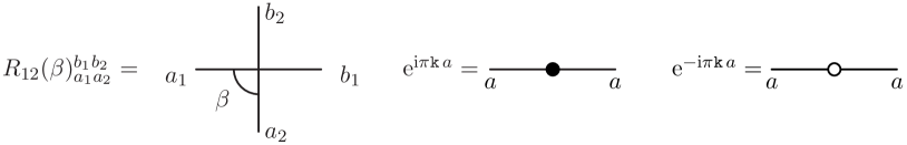
Figure 1: Graphical representation of the $R$-matrix (4) and the boundary twists $\mbox{e}^{\pm{\rm i}\pi{\mathtt{k}}\sigma_{z}}$. The edge indices $a,a_{1},a_{2},b_{1},b_{2}$ take two values $\pm 1$.

Then, with these conventions the transfer matrix is represented as in fig. 2.

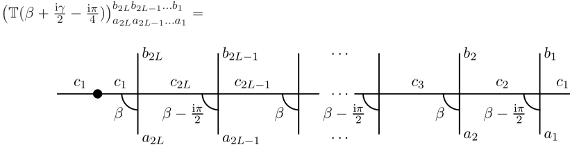
Figure 2: Graphical representation of the transfer matrix (5). The summation over the spin indices assigned to internal edges is assumed.

The system, thus defined, can be studied using the Bethe Ansatz (BA) approach and the corresponding equations read explicitly as Lieb:1967 ; Baxter:1971

$$\bigg{(}\frac{\cosh(2\beta_{j}+{\rm i}\gamma)}{\cosh(2\beta_{j}-{\rm i}\gamma)}\bigg{)}^{L}=-\mbox{e}^{-2{\rm i}\pi{\tt k}}\ \prod_{m=1}^{M}\frac{\sinh(\beta_{j}-\beta_{m}+{\rm i}\gamma)}{\sinh(\beta_{j}-\beta_{m}-{\rm i}\gamma)}\ .$$ (7)

For a chain of given length $2L$ every solution of the BA equations corresponds to an eigenstate of the Hamiltonian (On the scaling behaviour of the alternating spin chain) with energy

$$E=-\sum_{j=1}^{M}\ \frac{4\sin(2\gamma)}{\cosh(4\beta_{j})+\cos(2\gamma)}\ .$$ (8)

The number of Bethe roots, $M$, is related to the total spin, $\frac{1}{2}\,\sum_{j}\,\sigma^{z}_{j}$, which turns out to be a conserved quantity for the chain

$$M=L-S^{z}\ .$$ (9)

Along with the $U(1)$-symmetry generated by the total spin operator, the system admits the global ${\cal C}{\cal P}$-invariance that acts on the spins as

$${\cal C}{\cal P}\,\sigma^{{{\pm}}}_{m}\,{\cal C}{\cal P}=\sigma^{{{\mp}}}_{2L+1-m}\,,\ \ \ \ \ \ \ {\cal C}{\cal P}\,\sigma^{{{z}}}_{m}\,{\cal C}{\cal P}=-\sigma^{{{z}}}_{2L+1-m}\ \ \ \ \ \ (m=1,\ldots,2L)\ .$$ (10)

The latter intertwines the sectors with $+S^{z}$ and $-S^{z}$ so that, without loss of generality, we will focus our attention on the case with

$$M\leq L\ .$$

Another global symmetry is ${\cal C}{\cal P}{\cal T}$, which acts inside each sector with given spin $S^{z}$. It manifests itself in the BA equations as the invariance of the system (7) w.r.t. complex conjugation:

$${\cal C}{\cal P}{\cal T}\ :\ \ \ \ \ \ \ \ \ \beta_{j}\mapsto\beta_{j}^{*}\ \ \ \ \ \ \ \ \ ({\rm mod}\ {\rm i}\pi)\,.$$ (11)

The spin chain possesses yet another $\mathbb{Z}_{2}$-symmetry. The explicit formula for the operator, ${\cal D}\,:\ {\cal D}^{2}=1$, that generates it is not important for our purposes and can be found in the papers Saleur:1990vd ; Jacobsen:2005xz ; Ikhlef:2011ay (it is denoted by $C$ therein). This $\mathbb{Z}_{2}$-symmetry corresponds to the invariance of eq. (7) w.r.t. the transformation

$$\ \ \ \ {\cal D}\ :\ \ \ \ \ \ \ \ \ \beta_{j}\mapsto\beta_{j}+\tfrac{{\rm i}\pi}{2}\ \ \ \ \ \ \ ({\rm mod}\ {\rm i}\pi)\,.$$ (12)

The assigning of a scale dependence to the low energy stationary states is greatly facilitated by the existence of the BA equations and can be done along the following line. First of all, eq. (7) should be re-written in logarithmic form:

$$LP(\beta_{j})=2\pi\,I_{j}-2\pi{\tt k}-\sum_{m=1}^{M}\Theta(\beta_{j}-\beta_{m})\ ,$$ (13)

where

$$P(\beta)=\frac{1}{{\rm i}}\ \log\bigg{[}\frac{\cosh({\rm i}\gamma+2\beta)}{\cosh({\rm i}\gamma-2\beta)}\bigg{]}\ ,\qquad\Theta(\beta)=\frac{1}{{\rm i}}\ \log\bigg{[}\frac{\sinh({\rm i}\gamma-\beta)}{\sinh({\rm i}\gamma+\beta)}\bigg{]}\ ,$$ (14)

while $I_{j}$ are the so-called Bethe numbers which are integers or half-integers for $M$ odd or even respectively. In order to define the Bethe numbers unambiguously one should specify the branches of the multivalued functions (14). We do this by imposing the conditions

$$P(0)=\Theta(0)=0$$

and choosing the system of branch cuts as shown in fig. 3.

Figure 3: The complex $\beta$-plane displaying the branch cuts for the functions $P$ (left panel) and $\Theta$ (right panel) that are closest to the origin. Subsequent cuts are obtained by shifting this picture by ${\rm i}\pi N$ with integer $N$.

It is important to mention that our analysis is restricted to the spin chain with the parameter

$$0<\gamma<\frac{\pi}{2}\ .$$ (15)

In this case the set of Bethe numbers corresponding to the lowest energy state in the sector with spin $S^{z}$ is given by

$$I_{j}=-\tfrac{1}{2}\,(M+1)+j\ \ \ \ \ \ \ \ (j=1,2,\ldots,M)\,,$$ (16)

valid for any $L$ (the labeling of the Bethe roots is explained in the caption in fig. 4). It should be emphasized that the $\{I_{j}\}$ do not uniquely specify the solution of the BA equations. For example, in the case of the vacuum in the sector with given $S^{z}$ the Bethe roots are distributed along the lines $\Im m(\beta)=0,\frac{\pi}{2}\ ({\rm mod}\,\pi)$. For even $M$ the vacuum is non-degenerate and the Bethe roots are equally distributed along these lines while for $M$ odd, the vacuum is two fold degenerate corresponding to an excess of one of the roots with $\Im m(\beta_{j})=0$ or $\frac{\pi}{2}$. Notice that in the latter case, the vacua are related by the $\mathbb{Z}_{2}$-transformation (12). In fact, the BA equations (13) with Bethe numbers as in (16) admit solutions such that the difference between the number of roots with $\Im m(\beta_{j})=\frac{\pi}{2}$ and $\Im m(\beta_{j})=0$ is equal to $m$, where (for an illustration see fig. 4)

$$m=0,\,\pm 2,\,\pm 4,\ldots\ \ \ {\rm for}\ \ M{\rm\ even}\ ,\ \ \ \ \ \ \ \ \ \ m=\pm 1,\,\pm 3,\ldots\ \ \ {\rm for}\ \ M{\rm\ odd}\ .$$ (17)

In the rest of this note, to simplify the discussion, we make the technical assumption that $M$ is even.

Figure 4: The pattern of Bethe roots in the complex plane for $L=20$, $\gamma=\frac{\pi}{5}$, ${\tt k}=\frac{1}{10}$ and with $S^{z}=0$. The integers beside each point show the labeling of the roots $\beta_{j}$. The corresponding Bethe numbers are given by eq. (16). The left panel corresponds to the ground state for which the number of roots on the lines $\Im m(\beta)=0$ and $\frac{\pi}{2}$ are equal ($m=0$); whereas on the right panel there are two more roots on the upper line than the lower one, i.e., $m=2$.

The numerical solution of the BA equations (13) not only requires the specification of the Bethe numbers, but also a proper initial approximation for the positions of the Bethe roots. The latter turns out to be the most difficult part of the numerical procedure. In our studies we approached the problem in the following way. Starting with a spin chain for relatively small $L$ ($L\leq 12$ in our analysis), we performed the numerical diagonalization of the Hamiltonian. The latter is part of a family of commuting operators, of which a prominent r$\hat{{\rm o}}$le is played by the so-called $Q$-operator. Together with the eigenvalues of the Hamiltonian, we computed the corresponding eigenvalues of $Q$, which turn out to be polynomials w.r.t. the variable $\mbox{e}^{-2\beta}$. The zeroes of this polynomial coincide with $\mbox{e}^{-2\beta_{j}}$, where the $\beta_{j}$ solve the BA equations (7). Thus for each Bethe state, i.e., the stationary state which is simultaneously an eigenvector of the $Q$-operator, we were able to find the set $\{\beta_{j}\}$ and, using eq. (13) as a definition of the Bethe numbers, the corresponding $\{I_{j}\}$. The numerical values of the Bethe roots for some $L$ can be used to construct an initial approximation for the solution of the BA equations (13) with $L$ increased to $L+2$ for which the qualitative pattern of the roots remains the same. We found this to be a highly effective procedure for determining the RG flow of an individual Bethe state.

With the above method it is possible to study the scale dependence of various observables. Along with the energy $E(L)$ computed by means of eq. (8) we also focused on the eigenvalue of the so-called quasi-shift operator. This is an important observable that commutes with the Hamiltonian and was introduced in Ikhlef:2011ay . It is defined using the transfer matrix (5) as

$${\mathbb{B}}={\mathbb{T}}\big{(}\textstyle{\frac{{\rm i}}{2}(\gamma+\frac{\pi}{2})}\big{)}\big{[}{\mathbb{T}}\big{(}\textstyle{\frac{{\rm i}}{2}(\gamma-\frac{\pi}{2})}\big{)}\big{]}^{-1}\,.$$ (18)

Interestingly, this operator can be viewed as a transfer matrix of a homogeneous (not alternating) six vertex model on the $45\degree$-rotated regular square lattice with quasi-periodic boundary conditions. Indeed, with the conventions of fig. 1, the operator $\mathbb{B}$ can be represented as in fig. 5. In terms of the Bethe roots, the eigenvalues of $\mathbb{B}$ are given by

$$B(L)=\prod_{j=1}^{M}\frac{\cosh(2\beta_{j})-\sin(\gamma)}{\cosh(2\beta_{j})+\sin(\gamma)}\ .$$ (19)

Finally another useful characteristic of the flow is the product

$$\Pi(L)=\prod_{j=1}^{M}\,\mbox{e}^{4\beta_{j}}\ ,$$ (20)

which can be considered as the eigenvalue of an operator that appears naturally in the large-$\beta$ expansion of the $Q$-operator.

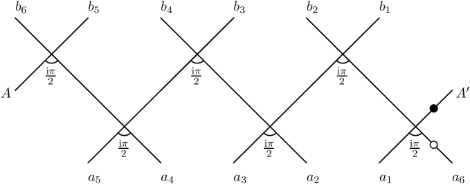
Figure 5: A graphical representation of the matrix elements $({\mathbb{B}})_{a_{2L}a_{2L-1}\ldots a_{1}}^{b_{2L}\,b_{2L-1}\ldots b_{1}}$ of the quasi-shift operator (18) for the chain of length $2L=6$. Summation over the spin indices assigned to internal edges is assumed. Note that for (quasi) periodic boundary conditions, $A$ and $A^{\prime}$ should be identified.

Before discussing the general features of $E(L)$, $B(L)$ and $\Pi(L)$, it is useful to get a feel of them for some particular classes of Bethe states. To this end, we restrict ourselves for now to the states with the simplest pattern of Bethe roots, illustrated in fig. 4, that were previously mentioned. The eigenvalue $B(L)$ for these states was already discussed in the literature Ikhlef:2011ay ; Candu:2013fva ; Frahm:2013cma . It was pointed out that for large $L$ the quantity

$$s(L)=\frac{n}{4\pi}\,\log(B)$$ (21)

with

$$n=\frac{\pi}{\gamma}-2>0$$

behaves as

$$s(L)\asymp\frac{\pi m}{4\log(L)}\,.$$ (22)

Here $m$ is the difference between the number of roots with $\Im m(\beta_{j})=\frac{\pi}{2}$ and $\Im m(\beta_{j})=0$ (17). The formula (22) resembles the quantization condition of a quantum mechanical particle in a potential well of length $\propto\log(L)$. It turns out, that as in usual quantum mechanics, a more accurate quantization condition is achieved by taking into account the phase shift that the particle picks up in the vicinity of the turning points. The results of our analysis yields the following quantization condition

$$8s\ \log\bigg{(}\frac{2L\Gamma(\frac{3}{2}+\frac{1}{n})}{\sqrt{\pi}\Gamma(1+\frac{1}{n})}\bigg{)}+\delta(s)-2\pi m=O\big{(}(\log L)^{-\infty}\big{)}\ .$$ (23)

The phase shift entering the above equation is explicitly given by the formula

$$\delta(s)=\frac{16s}{n}\ \log(2)-2{\rm i}\ \log\bigg{[}2^{4{\rm i}s}\ \frac{\Gamma(\frac{1}{2}+p-{{\rm i}s})\Gamma(\frac{1}{2}+{\bar{p}}-{{\rm i}s})}{\Gamma(\frac{1}{2}+p+{{\rm i}s})\Gamma(\frac{1}{2}+{\bar{p}}+{{\rm i}s})}\,\bigg{]}$$ (24)

with

$$p=\tfrac{1}{2}\,\big{(}S^{z}+{\tt k}\,(n+2)\big{)}\,,\qquad\bar{p}=\tfrac{1}{2}\,\big{(}S^{z}-{\tt k}\,(n+2)\big{)}\,.$$ (25)

The quantization condition holds true up to power law corrections in $L$, as indicated by the r.h.s. of eq. (23). The quality of the approximation is illustrated in tab. 1. Also, it should be noted that the phase shift (24) was essentially guessed in ref.Ikhlef:2011ay .

$L$	$s$ from eqs. (19) (21)	$s$ from eq. (23)	$\big{(}{\rm r.h.s.\ of}\ \eqref{quantC1}\big{)}\times L^{2}$
10	1.102443315	1.138091292	-75.8926
20	0.897548147	0.904491191	-75.6208
50	0.712588922	0.713466560	-76.4795
100	0.615519194	0.615709067	-76.9693
200	0.541653004	0.541694888	-77.3589
400	0.483644642	0.483654019	-77.6930
800	0.436891428	0.436893552	-77.9932

Table 1: In the second column the values of $s$ were obtained by solving the BA equations for increasing $L$ with the parameters $\gamma=\frac{\pi}{6}$ ($n=4$), ${\tt k}=\frac{1}{5}$, $S^{z}=4$, $m=4$ and then using eqs. (19) (21). These are compared with predictions coming from the quantization condition (23). In the last column $s$ obtained from the BA equations is substituted into the l.h.s. of eq. (23) to measure the corrections $O\big{(}(\log L)^{-\infty}\big{)}$. It indicates that for $n=4$ these corrections are of the order $L^{-2+\epsilon}$ with $\epsilon\to+0$.

The large-$L$ asymptotic of the eigenvalue $\Pi(L)$ is expressed in terms of $s=s(L)$ (21). The relation, again valid up to powers of $L$, explicitly reads as

$$\Pi(L)=\Omega\ \bigg{[}\frac{2L\,\Gamma\big{(}\frac{3}{2}+\frac{1}{n}\big{)}}{\sqrt{\pi}\,\Gamma\big{(}1+\frac{1}{n}\big{)}}\bigg{]}^{\frac{2n(\bar{p}-p)}{n+2}}\,\big{(}1+O\big{(}(\log L)^{-\infty}\big{)}\big{)}$$ (26)

with

$$\Omega=2^{2({\bar{p}}-p)}\ \ (n+2)^{\frac{4(\bar{p}-p)}{n+2}}\ \Bigg{[}\frac{\Gamma\big{(}1+\frac{2\bar{p}}{n+2}\big{)}\,\Gamma(1+2p)}{\Gamma\big{(}1+\frac{2p}{n+2}\big{)}\,\Gamma(1+2\bar{p})}\Bigg{]}^{2}\ \ \frac{\Gamma\big{(}\frac{1}{2}+\bar{p}+{\rm i}s\big{)}\,\Gamma\big{(}\frac{1}{2}+\bar{p}-{\rm i}s\big{)}}{\Gamma\big{(}\frac{1}{2}+p+{\rm i}s\big{)}\,\Gamma\big{(}\frac{1}{2}+p-{\rm i}s\big{)}}\,\ .$$ (27)

Of course, the above formula can be applied only for the specific class of Bethe states we have been currently focused on. Finally the excitation energy of these states above the ground state turns out to be

$$\Delta E(L)=\frac{2\pi v_{F}}{L}\bigg{(}\frac{p^{2}+{\bar{p}}^{2}}{n+2}+\frac{2s^{2}}{n}\bigg{)}+o\big{(}L^{-1}\big{)}\,,$$ (28)

where $s=s(L)$ and the Fermi velocity reads as

$$v_{\rm F}=\frac{2(n+2)}{n}\ .$$ (29)

The formula (28) suggests that the Bethe states under consideration flow to conformal primaries as $L\to\infty$, with scaling dimensions given by the term in the parenthesis in the r.h.s. However it follows from eq. (22) that the value of $s(L)$ tends to zero for large $L$ if $m$ is left unchanged. A non-trivial scaling limit can be achieved by increasing $|m|$ simultaneously with $L$ in such a way that $s$ is kept fixed. Then the scaling dimensions pick up a component labeled by this continuous parameter. Thus the CFT underlying the critical behaviour of the alternating spin chain possesses a continuous spectrum of scaling dimensions.

Spectroscopy of the low energy excitations of the alternating spin chain reveals another class of states which, as $L\to\infty$, flows to conformal primaries characterized by the pair of conformal dimensions $(\bar{\Delta},{\Delta})$ with

$$\Delta=\frac{p^{2}}{n+2}+\frac{s^{2}}{n}\,,\ \ \ \ \ {\bar{\Delta}}=\frac{{\bar{p}}^{2}}{n+2}+\frac{s^{2}}{n}$$ (30)

and

$$p=\tfrac{1}{2}\,\big{(}S^{z}+({\tt k}+{\tt w})\,(n+2)\big{)}\,,\qquad\bar{p}=\tfrac{1}{2}\,\big{(}S^{z}-({\tt k}+{\tt w})\,(n+2)\big{)}\,.$$ (31)

The last formula is analogous to eq. (25) but with ${\tt k}$ shifted by the integer ${\tt w}=\pm 1,\pm 2\ldots\$. Since the Hamiltonian is a periodic function of ${\tt k}$ (see eqs. (On the scaling behaviour of the alternating spin chain), (3)) the integer ${\tt w}$ enumerates the different bands of the spectrum. We will refer to the corresponding states as winding states.

Figure 6: The pattern of Bethe roots for the winding state with ${\tt w}=-1$, $S^{z}=0$ and $L=20$. With the labeling as shown, the corresponding Bethe numbers are given by the reference distribution (32). The value of the parameters for the plot were taken to be $\gamma=\frac{\pi}{5}$ and ${\tt k}=\frac{1}{30}$.

It is instructive to discuss the pattern of the Bethe roots for the winding states. It turns out that it depends significantly on the sign of the integer ${\tt w}$. In particular when the twist parameter ${\tt k}$ is positive, i.e., $0<{\tt k}<\frac{1}{2}$ the typical pattern for ${\tt w}=-1$ is shown in fig. 6. For this state $s(L)=0$ for any $L$ so that as $L\to\infty$ it flows to the conformal primary whose conformal dimensions are as in (30), (31) with $S^{z}=s=0$. The Bethe numbers in this case are given by

$$I_{j}^{({\rm vac})}=-\tfrac{1}{2}\,(M+1)+j-{\tt w}\,,\ \ \ \ j=1,2,\ldots,M$$ (32)

with ${\tt w}=-1$. This differs from eq. (16) by an overall shift by ${\tt w}$. To obtain a winding state with non-zero $s$, one should disbalance the number of roots on the lines $\Im m(\beta)=0$ and $\Im m(\beta)=\frac{\pi}{2}$ while keeping the Bethe numbers the same as in (32), similar to what was discussed for the case with ${\tt w}=0$. Also recall that the value of $S^{z}$ is related to the total number of Bethe roots (9). It is important to note that together with the formula for the excitation energy (28), the quantization condition (23) and the product rule (26) are valid for these states provided $p$ and ${\bar{p}}$ are taken as in (31).

The states with positive windings ${\tt w}=+1,+2,\ldots\,$($0<{\tt k}<\frac{1}{2}$) display some interesting phenomena. The Bethe state corresponding to ${\tt w}=+1$ and with $s(L)=0$ ($B(L)=1$) is depicted on the left panel in fig. 7. Again as $L\to\infty$ it flows towards the conformal primary having conformal dimensions (30), (31) with $S^{z}=s=0$ and ${\tt w}=+1$. For sufficiently large $L$ the Bethe numbers are given by $I_{j}^{({\rm vac})}+\delta I_{j}$, where the variations $\delta I_{j}$ from the “vacuum” distribution (32) are zero except for the following cases:

$$\delta I_{1}=-1\,,\ \ \ \ \ \ \ \delta I_{2}=+1\,,\ \ \ \ \ \ \ \delta I_{\frac{1}{2}M+1}=-1\,,\ \ \ \ \ \ \ \delta I_{\frac{1}{2}M+2}=+1$$ (33)

(recall that $M$ is assumed to be even).

Figure 7: The Bethe roots for the winding states with ${\tt w}=+1$, $m=0$, $S^{z}=0$ and $L=20$. The left panel corresponds to the state for which $s(L)=0$, while the state related to the right panel, despite the similar pattern, has non-zero $s(L)$. For both states the Bethe numbers are as in eqs. (32), (33). The value of the parameters were taken to be $\gamma=\frac{\pi}{5}$ and ${\tt k}=\frac{1}{25}$.

Apart from this, we observed another state having the same Bethe numbers and a similar pattern of Bethe roots, shown in the right panel of fig. 7, but with $s(L)\neq 0$. Remarkably the $L$ dependence of $s(L)$ is still captured by the quantization condition (23) with $m=0$. An important feature of this dependence, which is plotted in fig. 8, is that $s(L)$ vanishes at finite $L$. In fact, in addition to the state corresponding to the pattern depicted in the right panel of fig. 7, there is another state related to it by the $\mathbb{Z}_{2}$-transformation ${\cal D}$. The corresponding pattern is obtained by shifting the roots in accordance with eq. (12). These states form a doublet with the same energy but with opposite signs of $s$. Thus there are, indeed, three states corresponding to the three real solutions of the quantization condition (23) for $m=0$ and sufficiently small $L$. A simple examination of (23) shows that if $L$ is increased past the point where the three solutions merge at $s=0$, one solution remains trivial ($s(L)=0$) while the other two form a pure imaginary conjugated pair. This perfectly matches results obtained from the Bethe Ansatz. In the right panel of fig. 8 we compare $-{\rm i}s(L)<0$ taken from the BA solutions versus the prediction coming from the quantization condition. Notice that as $L\to\infty$ the value of $s(L)$ approaches a finite pure imaginary number which, as it follows from (23), (24) is given by

$$\lim_{L\to\infty}s(L)={\rm i}\,\big{(}\,\bar{p}+\tfrac{1}{2}-\big{[}\bar{p}+\tfrac{1}{2}\big{]}\,\big{)}\ ,$$ (34)

Figure 8: A plot of $s(L)$ coming from the quantization condition (23) for the case with ${\tt w}=+1$, $m=S^{z}=0$ with parameters $\gamma=\frac{\pi}{5}$ and ${\tt k}=\frac{1}{25}$. The left panel shows that $s(L)$ vanishes for finite $L$. The right panel continues the flow above the threshold, where $s$ becomes pure imaginary eventually reaching $s=-\frac{{\rm i}}{10}$ (see eq. (34)), shown by the dashed line, in the $L\to\infty$ limit. The data points represent $s$ obtained from the solution to the BA equations associated with the RG trajectory whose representative state at $L=20$ corresponds to the right panel of fig. 7.

where $[\ldots]$ stands for the integer part of $\bar{p}+\tfrac{1}{2}$. Thus we conclude that the CFT describing the scaling behaviour of the alternating spin chain must contain primary fields of conformal dimensions (30) with $s$ not only real, but also taking a discreet set of pure imaginary values at the very least.

The construction of other winding states with ${\tt w}=+1$ and real non-zero $s(L)$ is achieved by disbalancing the number of roots at $\Im m(\beta)=0$ and $\frac{\pi}{2}$, somewhat similar to what was mentioned before for negative ${\tt w}$. We illustrate the pattern of Bethe roots for such a state on the left panel of fig. 9. Notice that the flow $s(L)$ agrees with the quantization condition for $m=2$ (see the right panel of fig. 9).

Figure 9: On the left panel, the pattern of Bethe roots for the winding state with $S^{z}=0$, ${\tt w}=+1$ and $L=20$. Data for $s(L)$ computed from the solution to the BA equations for the corresponding RG trajectory is represented by the points in the graph on the right panel of the figure. The line is a plot of $s(L)$ coming from the quantization condition (23) with $m=2$. The parameters were taken to be $\gamma=\frac{\pi}{5}$ and ${\tt k}=\frac{1}{25}$.

The Bethe numbers for this state turn out to be different from the case with $m=0$ described by eqs. (32) and (33). Namely, the non-vanishing variations of the Bethe numbers from the vacuum distribution (32) are given by

$$\delta I_{1}=-1\,,\ \ \ \ \delta I_{2}=+1\,.$$ (35)

It should be remembered that the Bethe numbers depend on the choice of branches for the functions $P(\beta)$ and $\Theta(\beta)$ appearing in the BA equations (13). In particular, their values are sensitive to local deformations of the cuts depicted in fig. 3. For example, for the winding state with ${\tt w}=+1$ having Bethe numbers (32), (33), it is possible to arrange for all the $\delta I_{j}$ to be zero by a small deformation of the branch cuts. Moreover a shift of any one of the Bethe roots $\beta_{j}\to\beta_{j}+{\rm i}\pi$ changes the set $\{I_{j}\}$. Because of these ambiguities we do not have a clear picture of how to assign the Bethe numbers a priori to a particular Bethe state. Finally we have checked that for all the states discussed up till now, the product rule (26) is in excellent agreement with numerical data.

Figure 10: The Bethe roots for the state flowing to a conformal descendent of dimensions $(\bar{\Delta},\Delta+1)$. In this case the non-zero variations of the Bethe numbers from the reference distribution (32) are given by $\delta I_{\frac{M}{2}}=1$ (recall that $M$ is assumed to be even). Note that the set of Bethe roots obtained through the ${\cal C}{\cal P}{\cal T}$-transformation of the depicted set has $\delta I_{M}=1$. The value of the parameters used for the plot are $\gamma=\frac{\pi}{5}$, $S^{z}=0$, ${\tt k}=\frac{1}{20}$ and $L=20$.

Having described the low energy states of the spin chain that flow to the conformal primaries, we now turn to the Bethe states that scale to the conformal descendents characterized by the pair of conformal dimensions $(\bar{\Delta}+{\bar{N}},\Delta+N)$. Let’s first illustrate them in the case where the primary conformal dimensions $\bar{\Delta}$, ${\Delta}$ are given by eq. (30) with $s=0$ and $p=-\bar{p}=\frac{1}{2}(n+2)\,{\tt k}$, i.e., $S^{z}={\tt w}=0$. Note that the value of $s(L)$ for the “descendent” Bethe states, defined by (19), (21), turns out to be a complex number in general that becomes zero only in the limit $L\to\infty$. The pattern of Bethe roots corresponding to the state which flows to the conformal descendent with $(\bar{\Delta},\Delta+1)$ is shown in fig. 10. Applying the ${\cal C}{\cal P}{\cal T}$-transformation (11) one obtains another state characterized by the same pair of conformal dimensions.

Figure 11: The pattern of Bethe roots for the states flowing to the conformal descendent with $(\bar{\Delta},\Delta+2)$. The left panel corresponds to the ${\cal C}{\cal P}{\cal T}$-invariant state whose non-vanishing $\delta I_{j}$ are given by $\delta I_{\frac{M}{2}}=\delta I_{M}=1$. For the state corresponding to the right panel, one has $\delta I_{\frac{M}{2}-1}=\delta I_{\frac{M}{2}}=1$. The Bethe roots for the other three states of this type are obtained by the ${\cal C}{\cal P}{\cal T}$ (11) and ${\cal D}$ (12) transformations. The non-vanishing $\delta I_{j}$ for these three states are $\delta I_{M-1}=\delta I_{M}=1$ (${\cal D}$-transformed state) $\delta I_{M}=2$ (${\cal C}{\cal P}{\cal T}$-transformed state) and $\delta I_{\frac{M}{2}}=\delta I_{\frac{M}{2}+1}=1$ (${\cal C}{\cal P}{\cal T}$- and ${\cal D}$-transformed state). The values of the parameters used in the plot are $\gamma=\frac{\pi}{5}$, $S^{z}=0$ and ${\tt k}=\frac{1}{30}$.

At the second level with $(\bar{\Delta},\Delta+2)$ there exists a ${\cal C}{\cal P}{\cal T}$ -invariant state for which the typical pattern of Bethe roots is shown in the left panel of fig. 11. The roots corresponding to another state at this level are depicted on the right panel of the figure. Together with its ${\cal D}$-transform, these states form a doublet having the same complex energy. A doublet with the complex conjugated energy is obtained by means of the ${\cal C}{\cal P}{\cal T}$-transformation. In the $L\to\infty$ limit, the value of $s$ tends to zero, the energy becomes real and coincides for all five states. Of course, a similar picture holds true for the descendent Bethe states associated with the conformal dimensions $(\bar{\Delta}+1,\Delta)$ and $(\bar{\Delta}+2,\Delta)$.

The major r${\hat{\rm o}}$le in the analysis of the RG flow and the identification of the scaling limits of the Bethe states belongs to the quantization condition (23) and the product rule (26). The latter is especially important as it typically resolves all the degeneracies in the spectrum of the Hamiltonian. However there is no reason to expect that the phase shift $\delta(s)$ appearing in the quantization condition eq. (23) is the same for the descendent Bethe states as for those flowing to the conformal primaries (24). Of course, $\Omega$ entering the product rule (26) must also be modified. Our approach for determining the asymptotic formula for the product rule and the phase shift for the descendent Bethe states was based on the ODE/IQFT correspondence Dorey:1998pt ; Bazhanov:1998wj ; Suzuki:2000fc ; Bazhanov:2003ni .

Consider the second order ODE

$$\bigg{[}\,-\frac{\mbox{d}^{2}}{{\mbox{d}z}^{2}}+\frac{p^{2}-\frac{1}{4}}{z^{2}}+\frac{2{\rm i}s}{z}+1\,\bigg{]}\,\Psi=0$$ (36)

possessing two singular points – a regular singular point at $z=0$ and an irregular one at $z=\infty$. The coefficients of the equation are single valued in the vicinity of $z=0$. Thus for $p\neq 0,\pm\frac{1}{2},\pm 1,\ldots$, one can introduce a fundamental set of solutions $\Psi_{\pm p}(z)$ such that

$$\Psi_{\pm p}(z)\to z^{\frac{1}{2}\pm p}\ \ \ \ \ \ {\rm as}\ \ \ z\to 0\ ,$$ (37)

and the corresponding monodromy matrix along a small contour about zero is diagonal. We will assume that $p$ is a real number and without loss of generality we take it to be positive. For our purposes it is sufficient to focus on the solution $\Psi_{p}(z)$. In the vicinity of the irregular singular point it has the following behaviour

$$\Psi_{p}(z)\to\begin{cases}C^{(+)}_{p}\ (+z)^{+{\rm i}s}\ \mbox{e}^{+z}\ \ \ \ \ &{\rm as}\ \ \ \ \Re e(z)\to+\infty\\[5.69046pt] C^{(-)}_{p}\ (-z)^{-{\rm i}s}\ \mbox{e}^{-z}\ \ \ \ \ &{\rm as}\ \ \ \ \Re e(z)\to-\infty\end{cases}\ .$$ (38)

Since (36) is essentially the confluent hypergeometric equation, the formula for the connection coefficients $C^{(\pm)}_{p}$ is found in any standard textbook. Using the explicit expression, one observes that the phase shift $\delta$ (24) and the function $\Omega$ (27) can be represented in the form

$$\delta = \frac{16s}{n}\ \log(2)-2{\rm i}\log\Bigg{[}\,\frac{{C}^{(+)}_{p}\,{C}^{(+)}_{\bar{p}}}{{C}^{(-)}_{p}\,{C}^{(-)}_{\bar{p}}}\Bigg{]}$$

$$\Omega = (n+2)^{\frac{4(\bar{p}-p)}{n+2}}\ \Bigg{[}\frac{\Gamma(1+\frac{2{\bar{p}}}{n+2})}{\Gamma(1+\frac{2p}{n+2})}\Bigg{]}^{2}\ \ \frac{{C}^{(+)}_{p}\,{C}^{(-)}_{p}}{{C}^{(+)}_{\bar{p}}\,{C}^{(-)}_{\bar{p}}}\ .$$

It is well known that the ODE (36) is obtained from the hypergeometric equation, i.e., the Fuchsian differential equation with three regular singular points, through a certain limiting procedure. The same procedure can be applied to the so-called generalized hypergeometric oper introduced and studied in the work Bazhanov:2013cua . This allows one to determine formulae for $\delta$ and $\Omega$ analogous to (On the scaling behaviour of the alternating spin chain) that work for the descendent Bethe states. An account of the derivation is given below.

As the first step the ODE (36) is replaced by the following “generalized confluent hypergeometric equation”

$$\bigg{[}-\frac{\mbox{d}^{2}}{\mbox{d}z^{2}}+\frac{p^{2}-\frac{1}{4}}{z^{2}}+\frac{2{\rm i}s}{z}+1+\sum_{j=1}^{N}\bigg{(}\frac{2}{(z-w_{j})^{2}}+\frac{n_{j}}{z(z-w_{j})}\bigg{)}\,\bigg{]}\,\Psi=0\ .$$ (40)

Together with the singularities at $z=0$ and $z=\infty$, this equation contains an additional $N$ singular points characterized by the $2N$ complex parameters $(w_{j},n_{j})$. We require that the additional singularities are “apparent” or monodromy free, i.e., any solution of eq. (40) remains single valued in their vicinity. This requirement leads to a system of algebraic constraints imposed on the set $(w_{j},n_{j})$ which read explicitly as

$$c_{j}\,\big{(}\,\tfrac{1}{4}\,c_{j}^{2}-t_{0}^{(j)}\big{)}-t_{1}^{(j)}=0\qquad\qquad(j=1,2,\ldots,N)\,,$$ (41)

where $c_{j}=-n_{j}/w_{j}$ and

$$t_{0}^{(j)} = \frac{p^{2}-\frac{1}{4}}{w_{j}^{2}}+\frac{2{\rm i}s}{w_{j}}+1-\frac{n_{j}}{w_{j}^{2}}+\sum_{k\not=j}\bigg{(}\frac{2}{(w_{j}-w_{k})^{2}}+\frac{n_{k}}{w_{j}(w_{j}-w_{k})}\bigg{)}$$

$$t_{1}^{(j)} = -2\ \frac{p^{2}-\frac{1}{4}}{w_{j}^{3}}-\frac{2{\rm i}s}{w_{j}^{2}}+\frac{n_{j}}{w^{3}_{j}}-\sum_{k\not=j}\bigg{(}\frac{4}{(w_{j}-w_{k})^{3}}+\frac{n_{k}\,(2w_{j}-w_{k})}{w_{j}^{2}\,(w_{j}-w_{k})^{2}}\bigg{)}\ .$$

Assuming that the positions of the singularities $\{w_{j}\}$ are given, the above equations specify the value of the “accessory parameters” $\{n_{j}\}$. A remarkable property of this system is that the $\{n_{j}\}$, considered as functions of $\{w_{j}\}$, satisfy the integrability conditions

$$w_{j}\,\frac{\partial n_{k}}{\partial w_{j}}=w_{k}\,\frac{\partial n_{j}}{\partial w_{k}}\ .$$

This means that there exists the (multi-valued) generating function $f^{(N)}(w_{1},\ldots,w_{N})$ such that

$$n_{j}=-w_{j}\,\frac{\partial f^{(N)}}{\partial w_{j}}\ .$$ (42)

In the domain

$$|w_{1}|<|w_{2}|<\ldots<|w_{N}|\ ,$$

the function $f^{(N)}$ can be defined by supplementing (42) with the recursion

$$\lim_{w_{N}\to-\infty}f^{(N)}(w_{1},\ldots,w_{N})=f^{(N-1)}(w_{1},\ldots,w_{N-1})\ .$$ (43)

In particular,

$$f^{(N)}(w_{1},\ldots,w_{N})=\int_{{\cal C}(w_{N},\infty)}\frac{\mbox{d}w}{w}\ n_{N}(w_{1},\ldots,w_{N-1},w)+f^{(N-1)}(w_{1},\ldots,w_{N-1})\ .$$ (44)

The integration contour here starts at the point $w_{N}$ and goes to infinity in the complex $w$-plane. Its precise shape is not important but it must be chosen to ensure convergence of the integral, i.e., $n_{N}$ must vanish along ${\cal C}(w_{N},\infty)$:

$$\lim_{w\to\infty}n_{N}(w_{1},\ldots,w_{N-1},w)\big{|}_{w\in{\cal C}(w_{N},\infty)}=0\ .$$

Thus the generating function is defined unambiguously up to a single constant $f^{(0)}$ that does not depend on $\{w_{j}\}$ and, hence, can be set to zero:

$$f^{(0)}=0\ .$$ (45)

The relations (44), (45) are sufficient for the numerical computation of the generating function $f^{(N)}$, however we do not have a useful analytic formula except when $N=1$. In this case, as it follows from the algebraic equation (41), the pair of complex numbers $(w,n)\equiv(w_{1},n_{1})$ belong to the cubic

$$(n+2)\ \big{(}(n+1)^{2}-4p^{2}\big{)}-8{\rm i}s\,(n+1)\,w-4n\,w^{2}=0\ .$$ (46)

Explicit computation of the integral (44) yields

$$f^{(1)}=p\ \log\big{(}{\check{R}}^{(1)}\big{)}+{\rm i}s\,\log\big{(}\check{D}^{(1)}\big{)}-n+\frac{1}{2}\ \log\bigg{(}\,\frac{w^{4}}{4p^{2}}\ \big{(}1-{\check{R}}^{(1)}\big{)}\big{(}1/{\check{R}}^{(1)}-1\big{)}\bigg{)}\ ,$$ (47)

where

$${\check{R}}^{(1)} = \frac{(n+1+2p-2w)(n+1+2p+2w)}{(n+1-2p-2w)(n+1-2p+2w)}$$ (48)

$$\check{D}^{(1)} = \frac{(1+2p-2{\rm i}s)(1-2p-2{\rm i}s)}{(1+2p+2{\rm i}s)(1-2p+2{\rm i}s)}\ \ \frac{2nw-(n+2)(n-2{\rm i}\,s)}{2nw+(n+2)(n+2{\rm i}\,s)}\ .$$

Note that in the above formulae $n$ should be understood as a function of $w$ as dictated by the cubic equation (46). Also the partial derivatives of $f^{(1)}$ w.r.t. the parameters $p$ and $s$ can be conveniently expressed in terms of the functions ${\check{R}}^{(1)}$ and $\check{D}^{(1)}$ respectively:

$$\bigg{(}\frac{\partial f^{(1)}}{\partial p}\bigg{)}_{w,s}=\,\log\big{(}{\check{R}}^{(1)}\big{)}\,,\qquad\bigg{(}\frac{\partial f^{(1)}}{\partial s}\bigg{)}_{w,p}=\,{\rm i}\log\big{(}{\check{D}}^{(1)}\big{)}\ .$$ (49)

The subject of our interest are the connection coefficients $C^{(\pm,N)}_{p}$ for the generalized confluent hypergeometric equation (40) that are defined in the same way (37), (38) as for the original ODE (36). However now the connection coefficients are functions of the $N$ variables $\{w_{j}\}$ (and of course $s$ and $p$). The remarkable fact, which was discussed in the context of the generalized hypergeometric oper in Bazhanov:2013cua , is that

$$\frac{{C}_{p}^{(+,N)}}{{{C}}_{p}^{(-,N)}}=2^{2{\rm i}s}\ \frac{\Gamma(\frac{1}{2}+p-{\rm i}s)}{\Gamma(\frac{1}{2}+p+{\rm i}s)}\ \exp\bigg{(}-{\rm i}\,\frac{\partial{f^{(N)}}}{\partial s}\,\bigg{)}_{w_{j},p}$$ (50)

$${{C}}^{(+,N)}_{p}\,{{C}}^{(-,N)}_{p}=\frac{2^{-2p-1}\ \Gamma^{2}(1+2p)}{\Gamma(\frac{1}{2}+p-{\rm i}s)\Gamma(\frac{1}{2}+p+{\rm i}s)}\ \exp\bigg{(}\frac{\partial{f^{(N)}}}{\partial p}\,\bigg{)}_{w_{j},s}\ .$$

Up till now $\{w_{j}\}$ have been treated as the independent variables. In fact, for the problem at hand, it is useful to regard $\{n_{j}\}$ as independent, with $\{w_{j}\}$ considered as functions of this set defined through the algebraic system (41). In view of eq. (42) one can perform the Legendre transform of $f^{(N)}$ w.r.t. the variables $\{\log(w_{j})\}$. The result will be denoted by ${g}^{(N)}$:

$${g}^{(N)}(n_{1},\ldots,n_{N})=\sum_{j=1}^{N}n_{j}\,\log(w_{j})+f^{(N)}\ .$$ (51)

Here we emphasize the dependence of $g^{(N)}$ on the set $\{n_{j}\}$. It also depends on the parameters $s,p$ and, as follows from the general properties of the Legendre transform, the following substitution can be made in eq.(50)

$$\bigg{(}\frac{\partial{f^{(N)}}}{\partial s}\,\bigg{)}_{w_{j},p}=\bigg{(}\frac{\partial{{g}^{(N)}}}{\partial s}\bigg{)}_{n_{j},p}\ ,\ \ \ \ \ \ \ \bigg{(}\frac{\partial{f^{(N)}}}{\partial p}\,\bigg{)}_{w_{j},s}=\bigg{(}\frac{\partial{{g}^{(N)}}}{\partial p}\bigg{)}_{n_{j},s}\ ,$$ (52)

provided that the connection coefficients ${{C}}^{(\pm,N)}_{p}$ are understood as functions of the independent variables $\{n_{j}\}$.

Finally we need a clone of the ODE (40):

$$\bigg{[}-\frac{\mbox{d}^{2}}{\mbox{d}{\bar{z}}^{2}}+\frac{\bar{p}^{2}-\frac{1}{4}}{\bar{z}^{2}}+\frac{2{\rm i}s}{\bar{z}}+1+\sum_{j=1}^{\bar{N}}\bigg{(}\frac{2}{(\bar{z}-\bar{w}_{j})^{2}}+\frac{\bar{n}_{j}}{\bar{z}(\bar{z}-\bar{w}_{j})}\bigg{)}\bigg{]}\,{\Psi}=0\ .$$ (53)

This equation is only notationally different so that the corresponding connection coefficients are given similarly to (50),(52). Then, as a result of our analysis we obtained the following expression generalizing (On the scaling behaviour of the alternating spin chain)

$$\delta = \frac{16s}{n}\ \log(2)-2{\rm i}\log\Bigg{[}\,\frac{{C}^{(+,N)}_{p}\ \bar{{C}}^{(+,\bar{N})}_{\bar{p}}}{{C}^{(-,N)}_{p}\ \bar{{C}}^{(-,\bar{N})}_{\bar{p}}}\Bigg{]}\ \Bigg{|}_{n_{j}=\bar{n}_{j}=n}$$

$$\Omega = (n+2)^{\frac{4(\bar{p}-p)}{n+2}}\ \frac{\Gamma^{2}(1+\frac{2{\bar{p}}}{n+2})}{\Gamma^{2}(1+\frac{2p}{n+2})}\ \ \frac{{C}^{(+,N)}_{p}\ {C}^{(-,N)}_{p}}{\bar{{C}}^{(+,\bar{N})}_{\bar{p}}\ \bar{{C}}^{(-,\bar{N})}_{\bar{p}}}\ \Bigg{|}_{n_{j}=\bar{n}_{j}=n}\ .$$

In equation (On the scaling behaviour of the alternating spin chain) the variables $\{n_{j}\}$ and $\{\bar{n}_{j}\}$ are set to the same value $n$. From this point on ${C}^{(\pm,N)}_{p}$, $\bar{{C}}^{(\pm,\bar{N})}_{\bar{p}}$ will always be taken to mean the connection coefficients for the ODEs (40), (53) with the parameters $\{n_{j}\}$, $\{\bar{n}_{j}\}$ restricted in this way. Note that in this case the algebraic system (41) determining the position of the singularities $\{w_{j}\}$ simplifies to

$$4n\,w_{k}^{2}\!\! + \!\!8{\rm i}s\,(n+1)\,w_{k}-(n+2)\ \big{(}(n+1)^{2}-4p^{2}\big{)}$$

$$+ \!\!4\ \sum_{j\not=k}^{N}\frac{w_{k}\,(\,(n+2)^{2}\,w_{k}^{2}-n(2n+5)\,w_{k}w_{j}+n(n+1)\,w_{j}^{2}\,)}{(w_{k}-w_{j})^{3}}=0\ \ \ \ \ \ \ \ \ (k=1,\ldots,N)\ .$$

A similar equation holds with the set $\{w_{j}\}_{j=1}^{N}$ replaced by $\{\bar{w}_{j}\}_{j=1}^{\bar{N}}$ and $p$ substituted with $\bar{p}$.

In view of (50), (52), the structure of the formulae (On the scaling behaviour of the alternating spin chain) suggests the following re-writing

$$\delta = -2\,\bigg{(}\frac{\partial{G}^{(N)}}{\partial s}\bigg{)}_{n,p}-2\,\bigg{(}\frac{\partial{\bar{G}}^{({\bar{N}})}}{\partial s}\bigg{)}_{n,{\bar{p}}}$$ (56)

$$\Omega = \exp\Bigg{[}\bigg{(}\frac{\partial{G}^{(N)}}{\partial p}\bigg{)}_{n,s}-\bigg{(}\frac{\partial{\bar{G}}^{({\bar{N}})}}{\partial{\bar{p}}}\bigg{)}_{n,s}\,\Bigg{]}\ ,$$

where

$$G^{(N)}=G^{(0)}(s,p)+g^{(N)}|_{n_{j}=n}\ ,\ \ \ \ \ \ \ \ {\bar{G}}^{({\bar{N}})}=G^{(0)}(s,{\bar{p}})+{\bar{g}}^{({\bar{N}})}|_{\bar{n}_{j}=n}$$ (57)

and $G^{(0)}(s,p)$ is adjusted to make (56) valid in the case $N=\bar{N}=0$ with $g^{(0)}={\bar{g}}^{(0)}=0$. The straightforward calculation shows that for $\Re e(p)>-1,\ \Re e(p\pm{\rm i}s)>-\frac{1}{2}$, the function $G^{(0)}$ can be written as

$${G}^{(0)}(s,p) = \frac{1}{24}\,\log\Big{(}4^{n+1}\,n^{n}\,(n+2)^{-n-2}\Big{)}-\frac{2}{n}\ (n+1)\,s^{2}\ \log(2)$$

$$- n\int_{0}^{\infty}\frac{\mbox{d}t}{t}\ \Bigg{[}\,\frac{\mbox{e}^{-2pt}\sinh(\frac{nt}{2})}{2nt\,\sinh(t)\sinh(\frac{(n+2)t}{2})}+\frac{\mbox{e}^{-2pt}\sin^{2}(st)}{nt\,\sinh(t)}-\frac{1}{2(n+2)t^{2}}$$

$$+ \frac{p}{(n+2)\,t}+\bigg{(}\frac{1}{12}-\frac{p^{2}}{n+2}-\frac{s^{2}}{n}\bigg{)}\ \mbox{e}^{-t}\,\Bigg{]}\ .$$

The first term here in the r.h.s., independent of $p$ and $s$, is chosen for future convenience. Also note that the integral in (On the scaling behaviour of the alternating spin chain) is expressed in terms of the standard Barnes’ $G$-function.

Let’s illustrate the formula (On the scaling behaviour of the alternating spin chain) for the simplest Bethe states, which flow to the descendent with conformal dimensions $(\bar{\Delta},\Delta+1)$. In this case the relevant ODEs are (40) with one apparent singularity ($N=1$) and the confluent hypergeometric equation, i.e., (53) with $\bar{N}=0$. For given values of $n,p$ and $s$ the system (On the scaling behaviour of the alternating spin chain) boils down to a quadratic for $w\equiv w_{1}$ whose two solutions are:

$$w_{\pm}=-\frac{n+1}{2n}\,\Bigg{(}2{\rm i}\,s\pm\sqrt{n(n+2)}\ \sqrt{1-\frac{4p^{2}}{(n+1)^{2}}-\frac{4s^{2}}{n(n+2)}}\ \Bigg{)}\ .$$ (59)

The general relations (50), (On the scaling behaviour of the alternating spin chain) combined with the explicit formulae for $N=1$ (47)-(49) yields

$$\delta_{\pm} = -2{\rm i}\,\log\bigg{[}2^{\frac{4{\rm i}s}{n}(n+2)}\ \frac{\Gamma(\frac{1}{2}+p-{{\rm i}s})\Gamma(\frac{1}{2}+{\bar{p}}-{{\rm i}s})}{\Gamma(\frac{1}{2}+p+{{\rm i}s})\Gamma(\frac{1}{2}+{\bar{p}}+{{\rm i}s})}\ \frac{(1+2p-2{\rm i}s)(1-2p-2{\rm i}s)}{(1+2p+2{\rm i}s)(1-2p+2{\rm i}s)}$$ (60)

$$\times \frac{2nw_{\pm}-(n+2)(n-2{\rm i}\,s)}{2nw_{\pm}+(n+2)(n+2{\rm i}\,s)}\,\bigg{]}\,,$$

while

$$\Omega_{\pm} = 2^{2({\bar{p}}-p)}\ \ (n+2)^{\frac{4(\bar{p}-p)}{n+2}}\ \Bigg{[}\frac{\Gamma\big{(}1+\frac{2\bar{p}}{n+2}\big{)}\,\Gamma(1+2p)}{\Gamma\big{(}1+\frac{2p}{n+2}\big{)}\,\Gamma(1+2\bar{p})}\Bigg{]}^{2}\ \ \frac{\Gamma\big{(}\frac{1}{2}+\bar{p}+{\rm i}s\big{)}\,\Gamma\big{(}\frac{1}{2}+\bar{p}-{\rm i}s\big{)}}{\Gamma\big{(}\frac{1}{2}+p+{\rm i}s\big{)}\,\Gamma\big{(}\frac{1}{2}+p-{\rm i}s\big{)}}\,$$ (61)

$$\times \frac{(n+1+2p-2w_{\pm})(n+1+2p+2w_{\pm})}{(n+1-2p-2w_{\pm})(n+1-2p+2w_{\pm})}\ .$$

In our discussion of the RG flow we mentioned two states that become the conformal descendents with $(\bar{\Delta},\Delta+1)$ in the scaling limit. Fig. 10 illustrates the pattern of Bethe roots for one such state, while the second is related to the former by the ${\cal C}{\cal P}{\cal T}$-transformation. This is in agreement that for $N=1$ there are two solutions of (On the scaling behaviour of the alternating spin chain), labeled by the subscripts “$\pm$” in eqs. (59)-(61). It turns out that the state illustrated in fig. 10 corresponds to the case of “+” with the values of the parameters taken as in the caption. In the left panel of fig. 12 we compare the numerical data for $s(L)$ obtained using the BA equations with the predictions coming from the quantization condition (23), where $m=0$ and the phase shift is taken to be $\delta=\delta_{+}$ (60). Numerical results for $\Pi(L)$ (20) are compared with the analytical predictions (26) with $\Omega=\Omega_{+}$ (61) on the right panel of fig. 12.

Figure 12: The scale dependence of $s(L)$ (left panel) and $L^{\nu}\,\Pi(L)$ with $\nu=\frac{2n(p-\bar{p})}{n+2}$ (right panel) for the state flowing to the conformal descendent with dimensions $(\bar{\Delta},\Delta+1)$, whose typical pattern of Bethe roots is depicted in fig. 10. The points come from the solution of the BA equations, whereas the solid lines result from the analytic expressions (23), (60) for $s(L)$ and (26), (61) for $\Pi(L)$. Note that in the right panel, the solid line tends to the finite limit $L^{\nu}\,\Pi(L)\to 0.554918\ldots$ as $L\to\infty$. The integer $m$ entering into the quantization condition is chosen to be zero, while the values of the remaining parameters are $\gamma=\frac{\pi}{5}$, $S^{z}=0$ and ${\tt k}=\frac{1}{20}$ ($p=-\bar{p}=\frac{\tt k}{2}\,(n+2)$, $n=3$).

For the case with $N=2$ we found that for general $s,p$ and $n$, the algebraic equation (On the scaling behaviour of the alternating spin chain) possesses exactly five solutions up to the permutation $w_{1}\leftrightarrow w_{2}$. We have checked that these solutions correspond to the five Bethe states discussed before that flow to the descendents with conformal dimensions $(\bar{\Delta},\Delta+2)$. Unfortunately we were not able to derive explicit analytical expressions for $\Omega$ and the phase shift $\delta$ for $N=2$ similar to (60),(61). However eqs. (44), (50), (On the scaling behaviour of the alternating spin chain) are sufficient for their numerical computation. Some results of our analysis are presented in tab. 2

$L$	$s(L)$	$\delta(s)$	r.h.s. of eq. (23)
$20$	$-0.042685+0.271838\,{\rm i}$	$1.282157-6.469176\,{\rm i}$	$(1.9+4.8\,{\rm i})\times 10^{-1}$
$50$	$-0.038249+0.221127\,{\rm i}$	$1.297885-7.177411\,{\rm i}$	$(3.9+9.9\,{\rm i})\times 10^{-2}$
$100$	$-0.034314+0.196574\,{\rm i}$	$1.330870-7.529820\,{\rm i}$	$(1.1+2.9\,{\rm i})\times 10^{-2}$
$200$	$-0.030893+0.177611\,{\rm i}$	$1.362463-7.806222\,{\rm i}$	$(3.2+8.2\,{\rm i})\times 10^{-3}$
$400$	$-0.028035+0.162200\,{\rm i}$	$1.389822-8.033551\,{\rm i}$	$(0.9+2.3\,{\rm i})\times 10^{-3}$
$800$	$-0.025647+0.149325\,{\rm i}$	$1.413107-8.225372\,{\rm i}$	$(2.5+6.5\,{\rm i})\times 10^{-4}$

Table 2: The value of $s(L)$ here is listed for the Bethe state, which flows to the conformal descendent with dimensions $(\bar{\Delta},\Delta+2)$. This state is not the ${\cal C}{\cal P}{\cal T}$-invariant one and its typical pattern of Bethe roots is shown in the right panel of fig. 11. The phase shift $\delta(s)$ was computed using (On the scaling behaviour of the alternating spin chain), (50) with the function $f^{(2)}$ calculated numerically via eqs. (44), (45). The last column shows the r.h.s. of the quantization condition (23) with $m=0$, where $s$ and $\delta(s)$ are taken from the previous two columns. The parameters used for the table are $\gamma=\frac{2\pi}{9}$, ${\tt k}=\frac{1}{30}$ and $S^{z}=0$.

We expect that for general $N$ the number of solutions of the algebraic system (On the scaling behaviour of the alternating spin chain) (up to mutual permutations of the set $\{w_{j}\}$) coincides with the number of partitions of $N$ into integer parts of two kinds ${\tt p}_{2}(N)$:

$$\sum_{N=0}^{\infty}{\tt p}_{2}(N)\,q^{N}=\prod_{k=1}^{\infty}\,\frac{1}{(1-q^{k})^{2}}=1+2\,q+5\,q^{2}+10\,q^{3}+20\,q^{4}+36\,q^{5}+\ldots\ .$$ (62)

Our numerical work suggests that for sufficiently large $L$ the states in the low energy part of the spectrum ($\{|\psi\rangle\}$) can be characterized by $p=\tfrac{1}{2}\,\big{(}S^{z}+({\tt k}+{\tt w})\,(n+2)\big{)}$, $\bar{p}=\tfrac{1}{2}\,\big{(}S^{z}-({\tt k}+{\tt w})\,(n+2)\big{)}$, $s=s(L)$ as well as an unordered set of solutions to eq. (On the scaling behaviour of the alternating spin chain) and one to its barred counterpart. Furthermore, for large $L$ the Bethe states develop the following factorized structure:

$$|\psi\rangle\approx\big{|}\{\bar{w}_{j}\}_{j=1}^{\bar{N}}\big{\rangle}_{s,\bar{p}}\otimes\big{|}\{{w}_{j}\}_{j=1}^{{N}}\big{\rangle}_{s,p}\,\ \ \ \ \ \qquad\qquad(L\gg 1)\ ,$$ (63)

where $s=s(L)$ and the $L$ dependence is determined through the quantization condition (23) with the phase shift $\delta$ given by eq. (On the scaling behaviour of the alternating spin chain). With this hypothesis one can turn to the scaling limit. As was explained before, to take this limit the integer $m$ should be assigned an $L$ dependence such that $s$ is kept fixed as $L\to\infty$. An immediate question is: what are the range of values of $s$ that appear in the scaling limit? A simple-minded guess is that all real values are allowed. Even if this is true, the admissible set must also contain pure imaginary $s$ as we explained before (see, e.g., fig. 8). We are not in a position to answer this question in full at the moment.

Despite that the global restrictions on $s$ are unknown, assuming that the pair of parameters $(s,p)$ are admissible, the structure of the linear span of the chiral states of the form $|\{w_{j}\}_{j=1}^{N}\rangle_{s,p}$ seems to be clear. They form a highest weight representation of the $W_{\infty}$-algebra, which was studied in Bakas:1991fs , with central charge $c=\frac{2(n-1)}{n+2}$. The latter contains the holomorphic currents $W_{j}$ with Lorentz spins $j=2,3,\ldots\$. All of these currents can be produced from the operator product expansion of $W_{2}$ (which is the holomorphic component of the energy momentum tensor) and the current $W_{3}$. The highest weight representation is specified by the highest weights $(\Delta,\varpi)$, where $\Delta$ is the conformal dimension and $\varpi$ is the value of the zero mode of the $W_{3}$-current. In terms of $s$ and $p$ the parameterization of $\Delta$ is given by eq. (30), while in the proper normalization of the $W_{3}$-current,

$$\varpi=s\,\bigg{(}\frac{3np^{2}}{3n+4}-\frac{(2n+3)n}{4(3n+4)}+s^{2}\bigg{)}\ .$$ (64)

The corresponding $W$-module will be denoted by ${\cal V}_{s,p}$. All possible states of the form $\big{|}\{w_{j}\}_{j=1}^{N}\big{\rangle}_{s,p}$, where $N=0,1,\ldots$ and $\{w_{j}\}$ are an unordered set of solutions of eq. (On the scaling behaviour of the alternating spin chain), are expected to form a basis of ${\cal V}_{s,p}$.

Of course there are many ways to introduce a basis for ${\cal V}_{s,p}$. The special property of the states $\big{|}\{w_{j}\}_{j=1}^{N}\big{\rangle}_{s,p}$ is that they are consistent with a certain integrable structure of the $W_{\infty}$-algebra. The latter can be specified as follows; using the $W$-currents one can construct a commuting set of local Integrals of Motion (IM) $\{\mathbb{I}_{k}\}$ with spin $k=1,2,\ldots$ :

$$[\mathbb{I}_{k},\mathbb{I}_{j}]=0\ .$$

By local we mean that each $\mathbb{I}_{k}$ is given by an integral over the local density built out of the $W$-currents and their derivatives. All the local IM are simultaneously diagonalized in the basis $\big{|}\{w_{j}\}_{j=1}^{N}\big{\rangle}_{s,p}$ , i.e.,

$$\mathbb{I}_{k}\,\big{|}\{w_{j}\}_{j=1}^{N}\big{\rangle}_{s,p}=I_{k}^{(N)}({\bm{w}})\ \big{|}\{w_{j}\}_{j=1}^{N}\big{\rangle}_{s,p}\ ,$$ (65)

where the symbol ${\bm{w}}$ is a shortcut notation for a set $\{w_{j}\}$ that satisfies the system (On the scaling behaviour of the alternating spin chain). The eigenvalues of the first three IM read explicitly as

$${{I}}_{1}^{(N)}({\bm{w}}) = {I}^{(0)}_{1}\big{(}s,\sqrt{p^{2}+(n+2)N}\,\big{)}$$ (66)

$${{I}}_{2}^{(N)}({\bm{w}}) = {I}^{(0)}_{2}\big{(}s,\sqrt{p^{2}+(n+2)N}\,\big{)}+\frac{3{\rm i}\,n^{2}}{3n+4}\ \sum_{k=1}^{N}w_{k}$$

$${{I}}_{3}^{(N)}({\bm{w}}) = {{I}}^{(0)}_{3}\big{(}s,\sqrt{p^{2}+(n+2)N}\,\big{)}-\frac{4n^{2}}{(5n+6)\,(n+2)}\ \bigg{(}n\,\sum_{k=1}^{N}w^{2}_{k}-{\rm i}\,s\,(n+4)\,\sum_{k=1}^{N}w_{k}\bigg{)}\,,$$

where

$${{I}}^{(0)}_{1}(s,p) = -\tfrac{n}{12}+\tfrac{np^{2}}{n+2}+s^{2}=n\,\big{(}\Delta-\tfrac{1}{12}\big{)}$$

$${{I}}^{(0)}_{2}(s,p) = \tfrac{3np^{2}s}{3n+4}-\tfrac{(2n+3)ns}{4(3n+4)}+s^{3}=\varpi$$ (67)

$${{I}}^{(0)}_{3}(s,p) = \tfrac{n^{2}p^{4}}{(5n+6)(n+2)}-\tfrac{n^{2}p^{2}}{2(5n+6)}-\tfrac{n^{2}(n-6)(2n+3)}{240(5n+6)}+\tfrac{6np^{2}s^{2}}{5n+6}-\tfrac{(3n+4)ns^{2}}{2(5n+6)}+s^{4}\ .$$

A prominent r$\hat{{\rm o}}$le in the integrable structure belongs to the chiral $Q$-operator, which acts in the highest weight module ${\cal V}_{s,p}$. It is obtained from the lattice $Q$-operator by taking an appropriately defined scaling limit. The construction of this chiral operator will be presented elsewhere as it requires a detailed description of the $W_{\infty}$-algebra and its representations. However its eigenvalue, labeled by the set $\{w_{j}\}$ (see eq. (63)), can be described without much effort as it coincides with the connection coefficients of a certain ODE. The differential equation is given by

$$\Bigg{[}\,-\frac{\mbox{d}^{2}}{{\mbox{d}z}^{2}}+\frac{p^{2}-\frac{1}{4}}{z^{2}}+\frac{2{\rm i}s}{z}+1+\sum_{j=1}^{N}\bigg{(}\frac{2}{(z-w_{j})^{2}}+\frac{n}{z(z-w_{j})}\bigg{)}+\lambda^{-2-n}\ z^{n}\,\Bigg{]}\,\Psi=0\ ,$$ (68)

where as before the positions of the singularities $\{w_{j}\}_{j=1}^{N}$ satisfy the algebraic system (On the scaling behaviour of the alternating spin chain). The ODE (68) contains a term involving the spectral parameter $\lambda$. Formally setting $\lambda=\infty$ gives back eq. (40) with $n_{1}=\ldots=n_{N}=n$. For finite $\lambda$, since $n>0$, the term $\lambda^{-2-n}\ z^{n}$ is negligible as $z\to 0$. Thus, similar as in eq. (40), one can define the solution $\Psi_{p}$ with $p>0$ through the asymptotic condition

$$\Psi_{p}(z)\to z^{\frac{1}{2}+p}\ \ \ \ \ \ {\rm as}\ \ \ z\to 0\ .$$

For large $z$ the term $\lambda^{-2-n}\ z^{n}$ becomes dominant and we introduce another solution, which decays along the positive real axis, through the WKB asymptotic

$$\Xi(z)\to\Big{(}\frac{z}{\lambda}\Big{)}^{-\frac{n}{4}}\ \exp\bigg{(}-\frac{2}{n+2}\ \Big{(}\frac{z}{\lambda}\Big{)}^{\frac{n}{2}+1}\bigg{)}\ \ \ \ \ \ {\rm as}\ \ \ \ z\to+\infty$$

(here we make the technical assumption that $\lambda>0$ and $n>2$). The eigenvalue of the CFT $Q$-operator, depending on the spectral parameter $\lambda$, essentially coincides with the Wronskian $W[\Psi_{p},\Xi]=\Xi\,\partial_{z}\Psi_{p}-\Psi_{p}\,\partial_{z}\Xi$ of these two solutions. It is not difficult to show that

$$\lim_{\lambda\to 0}\,\lambda^{\frac{1}{2}-p}\ {W}[\Psi_{p},\Xi]=\sqrt{\frac{n+2}{\pi}}\ (n+2)^{\frac{2p}{n+2}}\,\Gamma(1+\tfrac{2p}{n+2})\ .$$

The last formula implies that $A_{p}(\lambda)$ defined as

$$A_{p}(\lambda)=\sqrt{\frac{\pi}{n+2}}\ (n+2)^{-\frac{2p}{n+2}}\ \ \frac{\lambda^{\frac{1}{2}-p}\ W[\Psi_{p},\Xi]}{\Gamma(1+\frac{2p}{n+2})}$$ (69)

satisfies the normalization condition

$$A_{p}(\lambda)\to 1\ \ \ \ \ \ \ {\rm for}\ \ \ \ \ \ \ \ \ \lambda\to 0\ .$$

It turns out that the connection coefficient $A_{p}(\lambda)$, up to a simple factor, coincides with the eigenvalue of the chiral counterpart of the lattice $Q$-operator. Up to the simple modification

$${\mathfrak{C}}^{(\pm,N)}_{p}=\sqrt{\frac{\pi}{n+2}}\ (n+2)^{-\frac{2p}{n+2}}\ \ 2^{1\pm\frac{2{\rm i}s}{n}}\ \ \frac{C_{p}^{(\pm,N)}}{\Gamma(1+\frac{2p}{n+2})}\ ,$$ (70)

the previously defined connection coefficients $C^{(\pm,N)}_{p}$ (50) along with the eigenvalues of the local IM (65)-(On the scaling behaviour of the alternating spin chain) appear in the large-$\lambda$ asymptotic of $A_{p}(\lambda)$:

$$A_{p}(\lambda) \asymp {\mathfrak{C}}^{(+,N)}_{p}\ \lambda^{+\frac{{\rm i}s(n+2)}{n}-p}\ \exp\Big{(}b_{-1}\,\lambda^{\frac{n+2}{n}}\Big{)}$$

$$\times \exp\bigg{(}\,\sum_{m=1}^{\infty}(-{\rm i})^{m+1}\ b_{m}\ {{I}}^{(N)}_{m}\ \lambda^{-\frac{(n+2)m}{n}}+\sum_{m=1}^{\infty}\,{\tilde{H}}^{(+,N)}_{m}\ \lambda^{-(n+2)m}\,\bigg{)}$$

for $\Re e(\lambda)\to+\infty$ and

$$A_{p}(\lambda) \asymp {\mathfrak{C}}^{(-,N)}_{p}\ (-\lambda)^{-\frac{{\rm i}s(n+2)}{n}-p}\ \exp\Big{(}b_{-1}\,(-\lambda)^{\frac{n+2}{n}}\Big{)}$$

$$\times \exp\bigg{(}\,\sum_{m=1}^{\infty}(+{\rm i})^{m+1}\,b_{m}\ {{I}}^{(N)}_{m}\ (-\lambda)^{-\frac{(n+2)m}{n}}+\sum_{m=1}^{\infty}\,{\tilde{H}}^{(-,N)}_{m}\ (-\lambda)^{-(n+2)m}\,\bigg{)}$$

for $\Re e(\lambda)\to-\infty$. Here we use the constants

$$b_{m} = 2^{m+1}\ \ \frac{\Gamma(\frac{1}{2}+\frac{n+1}{n}\,m)\Gamma(1-\frac{m}{n})}{2\sqrt{\pi}\,m\,(m+1)!}\ .$$

The formulae (On the scaling behaviour of the alternating spin chain), (On the scaling behaviour of the alternating spin chain) also contain the notation ${\tilde{H}}^{(\pm,N)}_{m}$, which stands for the eigenvalues of the so-called dual non-local IM. The latter are important elements of the integrable structure, but they will not be touched upon in this paper. Note that ${\mathfrak{C}}^{(\pm,N)}_{p}$ (70) are also the eigenvalues of certain non-local IM. In particular their product, up to an overall normalization depending on $s$ and $p$, coincide with the eigenvalue of the so-called reflection operator. The latter can be defined similarly as in Bazhanov:2013cua and of course commutes with the local IM:

$$[{\mathbb{R}},\mathbb{I}_{k}]=0\ .$$

The eigenvalue of the reflection operator,

$${\mathbb{R}}\,\big{|}\{w_{j}\}_{j=1}^{N}\big{\rangle}_{s,p}=R^{(0)}\ {\check{R}}^{(N)}({\bm{w}})\ \big{|}\{w_{j}\}_{j=1}^{N}\big{\rangle}_{s,p}\,,$$ (73)

is given by

$${\check{R}}^{(N)}({\bm{w}})=\frac{{C}^{(+,N)}_{p}\,{C}^{(-,N)}_{p}}{{C}^{(+,0)}_{p}\,{C}^{(-,0)}_{p}}$$ (74)

and

$$R^{(0)}=2^{-4p}\ (n+2)^{-\frac{8p}{n+2}}\ \ \Bigg{[}\frac{\Gamma(1-\frac{2p}{n+2})\,\Gamma(1+2p)}{\Gamma(1+\frac{2p}{n+2})\,\Gamma(1-2p)}\Bigg{]}^{2}\ \ \frac{\Gamma(\tfrac{1}{2}-p+{\rm i}s)\ \Gamma(\tfrac{1}{2}-p-{\rm i}s)}{\Gamma(\tfrac{1}{2}+p+{\rm i}s)\ \Gamma(\tfrac{1}{2}+p-{\rm i}s)}\ .$$ (75)

Along with the reflection operator one can consider the operator $\check{{\mathbb{D}}}$ whose eigenvalues,

$$\check{{\mathbb{D}}}\,\big{|}\{w_{j}\}_{j=1}^{N}\big{\rangle}_{s,p}=\check{D}^{(N)}({\bm{w}})\ \big{|}\{w_{j}\}_{j=1}^{N}\big{\rangle}_{s,p}\,,$$ (76)

are given by

$$\check{D}^{(N)}({\bm{w}})=\frac{{C}^{(+,N)}_{p}}{{C}^{(-,N)}_{p}}\ \frac{{C}^{(-,0)}_{p}}{{C}^{(+,0)}_{p}}\ .$$ (77)

It plays a special r${\hat{\rm o}}$le in calculation of the density of states in the continuous theory. Indeed, assuming that the integer $m$ is even, the quantization condition (23) supplemented by (On the scaling behaviour of the alternating spin chain), implies that the density of the descendent states with the conformal dimensions $({\bar{\Delta}}+{\bar{N}},\Delta+N)$ is related to the density of the conformal primaries, $\rho_{0}(s)$, as follows

$$\!\!\!\rho^{(N,{\bar{N})}}(s)={\tt p}_{2}(N)\,{\tt p}_{2}({\bar{N}})\ \rho_{0}(s)+\frac{1}{2\pi{\rm i}}\ \partial_{s}\Big{(}\,{\tt p}_{2}({\bar{N}})\,\log{\rm det}_{N}(\check{\mathbb{D}})+{\tt p}_{2}(N)\,\log{\rm det}_{\bar{N}}({\bar{\check{\mathbb{D}}}})\,\Big{)}.$$ (78)

Here ${\tt p}_{2}(N)$ is the number of partitions as in eq.(62) and the symbol $\det_{N}({\check{\mathbb{D}}})$ stands for the determinant of the operator ${\check{\mathbb{D}}}$ restricted to the subspace of chiral states with conformal dimension $\Delta+N$, i.e.,

$${\rm det}_{N}(\check{\mathbb{D}})=\prod_{\bm{w}}{\check{D}}^{(N)}({\bm{w}})$$

and similar for the barred counterpart. The density of the conformal primaries reads explicitly as

$$\rho_{0}(s)=\frac{2}{\pi}\ \Bigg{(}\!\log(L/L_{0})+\frac{1}{4{\rm i}}\ \partial_{s}\log\bigg{[}\ \frac{\Gamma(\frac{1}{2}+p-{{\rm i}s})\Gamma(\frac{1}{2}+{\bar{p}}-{{\rm i}s})}{\Gamma(\frac{1}{2}+p+{{\rm i}s})\Gamma(\frac{1}{2}+{\bar{p}}+{{\rm i}s})}\,\bigg{]}\,\Bigg{)}\ ,$$ (79)

where $1/L_{0}=\frac{4^{\frac{n+1}{n}}\Gamma(\frac{3}{2}+\frac{1}{n})}{\sqrt{\pi}\,\Gamma(1+\frac{1}{n})}$. It should be pointed out that eq.(79) was originally proposed in ref.Ikhlef:2011ay . As it follows from the formula (48), in the case $N=1$ one has

$$\vskip 12.0pt plus 4.0pt minus 4.0pt{\rm det}_{1}({\check{\mathbb{D}}})=\frac{(1+2p-2{\rm i}s)(1-2p-2{\rm i}s)}{(1+2p+2{\rm i}s)(1-2p+2{\rm i}s)}\ .$$ (80)

In principle it is possible to calculate ${\rm det}_{N}({\check{\mathbb{D}}})$ for higher levels. For example, for $N=2$ we found

$${\rm det}_{2}({\check{\mathbb{D}}})=\frac{(1+2p-2{\rm i}s)^{2}\,(1-2p-2{\rm i}s)^{2}\,(3+2p-2{\rm i}s)\,(3-2p-2{\rm i}s)}{(1+2p+2{\rm i}s)^{2}\,(1-2p+2{\rm i}s)^{2}\,(3+2p+2{\rm i}s)\,(3-2p+2{\rm i}s)}\ .$$ (81)

This illustrates the fact that the density of the conformal descendent states with the conformal dimensions $({\bar{\Delta}}+{\bar{N}},\Delta+N)$ does not coincide with ${\tt p}_{2}(N)\,{\tt p}_{2}({\bar{N}})\,\rho_{0}(s)$.

We are now in a position to discuss the finite size corrections to the energy spectrum of the alternating spin chain. The results of our analysis suggest that its critical behaviour is described by a certain CFT whose Hilbert space is built out of the irreducible (for general $n>0$) representations $\bar{{\cal V}}_{s,\bar{p}}\otimes{\cal V}_{s,p}$ of the left and right chiral $W_{\infty}$-algebras. As usual, the finite size corrections are captured by irrelevant perturbations of the critical Hamiltonian. In the case under consideration, these are strongly constrained due to the integrability of the spin chain with arbitrary length $L$. A useful property of the Hamiltonian (On the scaling behaviour of the alternating spin chain), which follows immediately from eq. (6), is that it can be written in the form

$$\mathbb{H}=\mathbb{H}^{(+)}+\mathbb{H}^{(-)}\,.$$

The operators $\mathbb{H}^{(\pm)}$ are related through the $\mathbb{Z}_{2}$-transformation ${\cal D}$ (12)

$$\mathbb{H}^{(\mp)}={\cal D}\,\mathbb{H}^{(\pm)}{\cal D}\,,$$

and read explicitly as

$$\mathbb{H}^{(+)} = \frac{1}{2}\,\tan(\gamma)\sum_{j=1}^{2L}\,\sigma^{z}_{j}\,\sigma^{z}_{j+1}-\frac{1}{\sin(2\gamma)}\,\sum_{j=1}^{L}\,\Big{(}\sigma^{x}_{2j}\,\sigma^{x}_{2j+2}+\sigma^{y}_{2j}\,\sigma^{y}_{2j+2}+\sigma^{z}_{2j}\,\sigma^{z}_{2j+2}\Big{)}$$ (82)

$$- \frac{{\rm i}}{2\cos(\gamma)}\,\sum_{j=1}^{L}\Big{(}\,\big{(}\sigma^{x}_{2j}\,\sigma^{y}_{2j+1}-\sigma^{y}_{2j}\,\sigma^{x}_{2j+1}\big{)}\,\sigma^{z}_{2j+2}+\sigma^{z}_{2j}\,\big{(}\sigma^{x}_{2j+1}\,\sigma^{y}_{2j+2}-\sigma^{y}_{2j+1}\,\sigma^{x}_{2j+2}\big{)}\Big{)}$$

$$+ L\,\cot(2\gamma)$$

and

$$\mathbb{H}^{(-)} = \frac{1}{2}\,\tan(\gamma)\sum_{j=1}^{2L}\,\sigma^{z}_{j}\,\sigma^{z}_{j+1}-\frac{1}{\sin(2\gamma)}\,\sum_{j=1}^{L}\,\Big{(}\sigma^{x}_{2j-1}\,\sigma^{x}_{2j+1}+\sigma^{y}_{2j-1}\,\sigma^{y}_{2j+1}+\sigma^{z}_{2j-1}\,\sigma^{z}_{2j+1}\Big{)}$$ (83)

$$+ \frac{{\rm i}}{2\cos(\gamma)}\,\sum_{j=1}^{L}\Big{(}\,\big{(}\sigma^{x}_{2j-1}\,\sigma^{y}_{2j}-\sigma^{y}_{2j-1}\,\sigma^{x}_{2j}\big{)}\,\sigma^{z}_{2j+1}+\sigma^{z}_{2j-1}\,\big{(}\sigma^{x}_{2j}\,\sigma^{y}_{2j+1}-\sigma^{y}_{2j}\,\sigma^{x}_{2j+1}\big{)}\Big{)}$$

$$+ L\,\cot(2\gamma)\ .$$

All three operators commute and can be diagonalized simultaneously. The eigenvalues $E^{(\pm)}$ of $\mathbb{H}^{(\pm)}$ are expressed in terms of the solution to the BA equations as

$${E}^{(+)}=-\sum_{j=1}^{M}\frac{2{\rm i}\sin(\gamma)}{\sinh(2\beta_{j})+{\rm i}\cos(\gamma)}\,,\qquad{E}^{(-)}=\sum_{j=1}^{M}\frac{2{\rm i}\sin(\gamma)}{\sinh(2\beta_{j})-{\rm i}\cos(\gamma)}\ .$$ (84)

Contrary to the Hamiltonian $\mathbb{H}$, the difference $\mathbb{H}^{(+)}-\mathbb{H}^{(-)}$ is odd w.r.t. the transformation ${\cal D}$. This imposes heavy restrictions on the finite size corrections to $E^{(+)}-E^{(-)}$ for the Bethe states of the form (63). Namely, the leading large-$L$ behaviour is described by the formula

$$\frac{{E}^{(+)}-{E}^{(-)}}{v_{\rm F}}=-\frac{2\pi{\rm i}}{L^{2}}\ g_{2}\,\big{(}I_{2}^{(N)}-\bar{I}_{2}^{(\bar{N})}\big{)}+o\big{(}L^{-2}\big{)}$$ (85)

with $I_{2}^{(N)}$ from eqs. (66), (On the scaling behaviour of the alternating spin chain) and the Fermi velocity is given by (29). The constant $g_{2}$ can be computed along the lines of Lukyanov:1997wq and reads explicitly as

$$g_{2}=\frac{\sqrt{\pi}\,\Gamma(\frac{5}{2}+\frac{2}{n})\Gamma^{2}(1+\frac{1}{n})}{3\Gamma(\frac{2}{n})\Gamma^{2}(\frac{3}{2}+\frac{1}{n})}\,.$$

In practice eq. (85) is useful for determining the scaling counterpart, i.e., the r.h.s. of eq. (63), for the Bethe state $|\psi\rangle$ even on the lattice of size $L\sim 10$, where all three $2^{2L}\times 2^{2L}$-matrices $\mathbb{H}$, $\mathbb{H}^{(\pm)}$ can be diagonalized directly. On the left panel of fig.13, we illustrate formula (85) for the state that as $L\to\infty$ flows to the conformal descendent with dimensions $(\bar{\Delta},\Delta+1)$.

Figure 13: The points represent numerical data for $\delta E_{{\rm odd}}\equiv E^{(+)}-E^{(-)}$ and $\delta E_{{\rm even}}\equiv E^{(+)}+E^{(-)}-\,v_{\rm F}\,e_{\infty}L$, which was computed using the Bethe roots for the state flowing to the conformal descendent with dimensions $(\bar{\Delta},\Delta+1)$. The typical pattern of roots for this state is given in fig. 10. On the left panel, the solid line is the prediction coming from the finite size corrections eq. (85). On the right panel, the asymptotic formula (On the scaling behaviour of the alternating spin chain) with only the $L^{-1}$ term included is displayed by the dashed line, while the solid line takes into account the $L^{-3}$ correction. The limiting value $\lim_{L\to\infty}\frac{L}{2\pi v_{\rm F}}\,\delta E_{{\rm even}}=0.839583\ldots$ is shown by the dotted line. Finally $s(L)$, which is needed to compute the r.h.s. of eqs. (85), (On the scaling behaviour of the alternating spin chain), was calculated using the quantization condition (23) with $\delta=\delta_{+}$ (60). The parameters were taken to be $S^{z}=0$, $m=0$, ${\tt w}=0$, $\gamma=\frac{\pi}{5}$ and ${\tt k}=\frac{1}{20}$.

It is possible to extract the finite size corrections for $E={E}^{(+)}+{E}^{(-)}$ from the results of the work Lukyanov:1997wq . In particular, one has that for $n>1$

$$\frac{{E}^{(+)}+{E}^{(-)}}{v_{\rm F}} = \,e_{\infty}\,L+\frac{2\pi}{nL}\ \Big{(}I_{1}^{(N)}+\,\bar{I}_{1}^{(\bar{N})}\,\Big{)}$$

$$- \frac{2\pi}{L^{3}}\ \Big{(}\,2\pi^{2}\,g_{1}I_{1}^{(N)}\,\bar{I}_{1}^{(\bar{N})}+g_{3}\,\big{(}\,{I}_{3}^{(N)}+{{\bar{I}}}_{3}^{(\bar{N})}\,\big{)}\,\Big{)}+O\big{(}L^{-5},L^{-2n-1}\big{)}\ .$$

Again the eigenvalues of the local IM $I_{1}^{(N)}$, $I_{3}^{(N)}$ are given in eqs. (66), (On the scaling behaviour of the alternating spin chain). The specific bulk energy $e_{\infty}$ reads as

$$e_{\infty}=-\frac{4}{\pi}\int_{0}^{\infty}\mbox{d}t\ \frac{\sinh(\frac{2t}{n})}{\sinh(\frac{(n+2)t}{n})\cosh(t)}\ ,$$

while the value of the constants are

$$g_{1}=-\frac{\cot(\frac{\pi}{n})}{2\pi\,n^{2}}\,,\ \ \ \ \ \ \ \ \ \ \ g_{3}=\frac{\pi\Gamma(\frac{7}{2}+\frac{3}{n})\Gamma^{3}(1+\frac{1}{n})}{18\Gamma(\frac{3}{n})\Gamma^{3}(\frac{3}{2}+\frac{1}{n})}\ .$$

Figure 14: Numerical data obtained from the solution to the BA equations for the winding states with ${\tt w}=1$, $S^{z}=0$, $m=0$ (left panel) and $m=2$ (right panel) is depicted for $\delta E\equiv E-\,v_{\rm F}\,e_{\infty}L$. On the left panel the crosses and circles correspond to the RG trajectories whose representatives for $L=20$ are shown on the left and right of fig. 7, respectively. On the right panel, the points correspond to the state whose typical pattern of Bethe roots is displayed in fig. 9. Note that $L$ ranges from $L=8$ to $L=1000$. In both panels the dashed lines come from the asymptotic formula eq. (On the scaling behaviour of the alternating spin chain) taking account only the $L^{-1}$ terms, while to compute the solid lines the $L^{-3}$ correction was included. The dotted horizontal lines show the limiting values of $\frac{L}{2\pi v_{\rm F}}\,\delta E$. The value of $s(L)$ entering into the r.h.s. of eq. (On the scaling behaviour of the alternating spin chain) was calculated using the quantization condition (23) with $m=0$ (left panel) and $m=2$ (right panel). The parameters are set to be the same as in fig. 7, i.e., $\gamma=\frac{\pi}{5}$ and ${\tt k}=\frac{1}{25}$.

The formula (On the scaling behaviour of the alternating spin chain) calls for some important remarks. Firstly, with regards to the symbol $O\big{(}L^{-5},L^{-2n-1}\big{)}$, by this notation we mean that

$$O(L^{-a},L^{-b})\equiv o(L^{-c})\ \ \ \ \ \ {\rm where}\ \ \ \ c={\rm min}(a,b)-\epsilon\ \ \ \ \ \ \ \forall\ \epsilon>0\ .$$ (87)

Corrections to (On the scaling behaviour of the alternating spin chain) proportional to integer powers of $L$ are expressed in terms of the eigenvalues of the local IM. The next correction of this kind will involve combinations of the eigenvalues of $\mathbb{I}_{m}$ and $\bar{\mathbb{I}}_{m}$ with $m\leq 5$. The term $\propto L^{-2n-1}$ comes from the dual non-local IM whose eigenvalue appeared in eqs. (On the scaling behaviour of the alternating spin chain), (On the scaling behaviour of the alternating spin chain) where it was denoted by $\tilde{H}_{1}^{(\pm,N)}$. For $0<n<1$ it becomes the dominant correction to the scaling, hence the restriction $n>1$ to the applicability of eq. (On the scaling behaviour of the alternating spin chain). The same happens in the $XXZ$ spin chain (see ref. Lukyanov:1997wq ). The next remark concerns the finite size corrections to the quantization condition (23), which was denoted by $O\big{(}(\log L)^{-\infty}\big{)}$. In fact, we have numerically checked that it goes as $O(L^{-2},L^{-2n})$ (see, e.g., tab. 1). It is easy to see that such an uncertainty in “$s$” will interfere with the subleading corrections presented in (On the scaling behaviour of the alternating spin chain). At first glance, this makes the $L^{-3}$ correction useless. However, in our numerical studies we found that formula (On the scaling behaviour of the alternating spin chain) gives remarkably accurate results not only when “$s$” is zero identically, but also for non-zero $s$ satisfying the quantization condition with $m=0$ (see right panel of fig. 13 and left panel of fig. 14). Note that for $m$ different from zero eq. (On the scaling behaviour of the alternating spin chain) sometimes gives reasonable results as shown on the right panel of fig. 14, where $m=2$. Unfortunately it is difficult to say a priori when the $L^{-3}$ term improves the accuracy of the leading asymptotic behaviour.

It should be mentioned that the quantization condition (23), (On the scaling behaviour of the alternating spin chain), the formula for $\Pi(L)$ (26), (On the scaling behaviour of the alternating spin chain), and the scaling of the energy (On the scaling behaviour of the alternating spin chain), which are the main tools enabling a detailed investigation of the RG flow, can be written in an elegant and compact way. To this end introduce the notation

$${\mathfrak{Y}}(L)=\bigg{(}{\frac{1}{6}-\frac{2s^{2}}{n}-\frac{p^{2}+{\bar{p}}^{2}}{n+2}-N-{\bar{N}}}\bigg{)}\log(L)+{\mathfrak{Y}}_{0}\ ,$$ (88)

where

$${\mathfrak{Y}}_{0}=\bigg{(}{\frac{1}{6}-\frac{2s^{2}}{n}-\frac{p^{2}+{\bar{p}}^{2}}{n+2}-N-{\bar{N}}}\bigg{)}\log\bigg{(}\frac{2\Gamma(\frac{3}{2}+\frac{1}{n})}{\sqrt{\pi}\Gamma(1+\frac{1}{n})}\bigg{)}+\frac{1}{n}\,\big{(}G^{(N)}+{\bar{G}}^{({\bar{N}})}\big{)}\ ,$$ (89)

and $G^{(N)}$, ${\bar{G}}^{({\bar{N}})}$ were defined before through eqs.(57),(On the scaling behaviour of the alternating spin chain). It is easy to see that the quantization condition takes the form

$$-2n\,\bigg{(}\frac{\partial{\mathfrak{Y}}}{\partial s}\bigg{)}_{{\tt k},L}=2\pi m+O(L^{-2},L^{-2n})\ \ \ \ \ \qquad(m=0,\pm 1,\pm 2,\ldots)\ ,$$ (90)

while

$$\Pi(L)=\exp\Bigg{[}\frac{2n}{n+2}\ \bigg{(}\frac{\partial{\mathfrak{Y}}}{\partial{\tt k}}\bigg{)}_{s,L}+O(L^{-2},L^{-2n})\,\Bigg{]}$$ (91)

and the equation for the energy (On the scaling behaviour of the alternating spin chain) is expressed as

$$\frac{E}{v_{\rm F}}-e_{\infty}\,L=-2\pi\ \bigg{(}\frac{\partial{\mathfrak{Y}}}{\partial L}\bigg{)}_{s,{\tt k}}+O(L^{-3},L^{-2n-1})\ .$$ (92)

The above relations point to the fundamental r$\hat{\rm{o}}$le of the quantity ${\mathfrak{Y}}$. In the following we will try to elucidate its meaning.

As it was first observed by Yang and Yang for the XXZ spin chain Yang1 ; Yang2 , the BA equations are obtained from a certain variational principle. In the case under consideration the latter is formulated as follows. Introduce the Yang-Yang functional defined for an arbitrary set of complex numbers $\{\beta_{j}\}$

$$Y\big{[}\{\beta_{j}\}\big{]}=\frac{n+2}{n}\ \bigg{[}\,2\sum_{j}\big{(}L\,v(\beta_{j})+({\tt k}-I_{j})\,\big{(}\beta_{j}-\tfrac{{\rm i}\pi}{4}\big{)}\,\big{)}+\sum_{j,m}u(\beta_{j}-\beta_{m})\,\bigg{]}\ ,$$ (93)

where the functions $u(\beta)$ and $v(\beta)$ are related to $\Theta(\beta)$ and $P(\beta)$ in (14) as

$$\Theta(\beta)=2\pi\ \partial_{\beta}u(\beta)\ ,\ \ \ \ \ P(\beta)=2\pi\ \partial_{\beta}v(\beta)\ .$$ (94)

The BA equations (13) are equivalent to the condition for a local extremum

$$\delta Y\big{[}\{\beta_{j}\}\big{]}=0\ ,$$

where all the parameters, including the set of the Bethe numbers $\{I_{j}\}$, are given and kept fixed under the infinitesimal variation of $\beta_{j}$. Suppose now we have a set $\{\beta_{j}\}$ solving the extremum condition, and consider the value of the Yang functional calculated on it. This on-shell value will be denoted below by $Y(L)$ emphasizing its dependence on the length of the spin chain. As it is sensitive to the shift $\beta_{j}\to\beta_{j}+{\rm i}\pi$ of any one of the Bethe roots, to define $Y(L)$ unambiguously we assume that $0\leq\Im m(\beta_{j})<\pi$. Notice that eq.(94) specifies the functions $u(\beta)$ and $v(\beta)$ up to additive constants, which have no effect on the extremum condition, but the on-shell value of the Yang functional depends on them. It will be convenient for us to define $u(\beta)$ as

$$u(\beta)=\frac{{\rm i}}{4\pi}\,\bigg{(}2\beta^{2}-\frac{\pi^{2}}{3}+\gamma(\pi-2\gamma)+\rm{Li}_{2}\big{(}\mbox{e}^{2\beta-2{\rm i}\gamma}\big{)}+\rm{Li}_{2}\big{(}\mbox{e}^{-2\beta-2{\rm i}\gamma}\big{)}\bigg{)}\ .$$ (95)

Here ${\rm{Li}}_{2}(z)$ is a dilogarithm function, with the standard choice of branch cut along the positive real axis $(1,+\infty)$ so that $u(\beta)$ is a single valued function in the complex plane $\beta$ with the systems of cuts shown in the right panel of fig. 3. Next, we specify the function $v(\beta)$ by the formula

$$v(\beta)=-\frac{1}{4\pi}\ \Im m\Big{(}{\rm{Li}}_{2}\big{(}-\mbox{e}^{2{\rm i}\gamma}\big{)}\Big{)}+\int_{0}^{\beta}\frac{\mbox{d}\beta^{\prime}}{2\pi}\,P(\beta^{\prime})\ ,$$ (96)

where the integration is taken along a straight line segment in the complex plane that connects the origin with the end point $\beta$. Thus defined, $v(\beta)$ is a single valued analytic function in the complex $\beta$-plane with two branch cuts starting from the points $+\frac{\pi-2\gamma}{4}\,{\rm i}$ and $-\frac{\pi-2\gamma}{4}\,{\rm i}$ which extend along the imaginary axis to $+{\rm i}\,\infty$ and $-{\rm i}\,\infty$, respectively. With this prescription there is an ambiguity in the computation of $v(\beta_{j})$ for the Bethe roots lying exactly on the imaginary axis with $|\Im m(\beta_{j})|\geq\frac{\pi-2\gamma}{4}$. However for a general value of the twist parameter ${\tt k}\not=0$, this subtlety can be ignored.

Consider the large-$L$ behaviour of $Y(L)$, i.e., the on-shell value of the Yang functional. It is not difficult to see that it diverges quadratically as $L\to\infty$,

$$Y(L)=Y^{\rm(div)}(L)+O\big{(}\log(L)\big{)}$$

with the divergent part involving the quadratic and linear terms

$$Y^{\rm(div)}(L)=y_{\infty}\,\frac{L^{2}}{4}+\frac{{\rm i}\pi}{n}\ {\cal N}\,L\ .$$ (97)

Notice that $Y^{({\rm div})}(L)$ is somewhat non-universal. In particular, $y_{\infty}$ depends on our voluntaristic choice of the integration constants appearing in the definition of $u(\beta)$ and $v(\beta)$. Specifying these functions as in (95), (96), it is straightforward to show that Lukyanov:2011wd

$$y_{\infty}=-\int_{0}^{\infty}\frac{\mbox{d}t}{t^{2}}\ \bigg{(}\frac{\sinh(\frac{2t}{n})}{\sinh(\frac{(n+2)t}{n})\cosh(t)}-\frac{2}{n+2}\bigg{)}\ .$$

It turns out that for such $u$ and $v$ the linear divergent part in (97) is pure imaginary with ${\cal N}$ an integer. The latter is sensitive to local deformations of the branch cuts for the function $v$ and hence is not particularly interesting. We can ignore this term by focusing on

$$\exp\big{(}2n\,Y^{({\rm reg})}(L)\big{)}=\exp\big{(}2n(Y(L)-Y^{\rm(div)}(L))\big{)}$$ (98)

instead of the Yang functional itself. There exists a remarkable relation between the quantity $\exp\big{(}2n\,Y^{({\rm reg})}(L)\big{)}$ and ${\mathfrak{Y}}(L)$ introduced in eq.(88). Namely

$$\exp\big{(}2n\,Y^{\rm(reg)}(L)\big{)}=\mbox{e}^{2\pi{\rm i}\,(n+2)\,({\tt k}\,{\cal N}_{1}+2\,{\cal N}_{2})}\ \exp\Big{(}2n\,{\mathfrak{Y}}(L)+2\pi ms+O(L^{-2},L^{-2n})\Big{)}\ .$$ (99)

Here the variable $s$ is defined by (19), (21) and is related to the integer $m$ through the quantization condition (90), while ${\cal N}_{1}$ and ${\cal N}_{2}$ appearing in the phase factor are integers. The value of these last two depends on the specification of the branch of the multi-valued function $\mathfrak{Y}_{0}$ (89) entering the r.h.s. of eq. (99) via $\mathfrak{Y}(L)$. Note that as it follows from the formula (91) for $\Pi(L)\equiv\prod_{j}\mbox{e}^{4\beta_{j}}$ and eq. (99) one has

$$\prod_{j=1}^{M}\,\mbox{e}^{2(\beta_{j}-\frac{{\rm i}\pi}{4})}=(-1)^{{\cal N}_{1}}\,\exp\Bigg{[}\frac{n}{n+2}\ \bigg{(}\frac{\partial{\mathfrak{Y}}}{\partial{\tt k}}\bigg{)}_{s,L}+O(L^{-2},L^{-2n})\,\Bigg{]}$$ (100)

(recall that in this paper $L$ and $M$ are assumed to be even). Also our numerical work shows that there is no simple relation between the vanishing as $L\to\infty$ corrections $O(L^{-2},L^{-2n})$ for $Y(L)$ and the corrections for the energy $E(L)$ indicated in (92). Thus it is unlikely that there is a simple formula that systematically relates the large-$L$ asymptotic expansions of $Y(L)$ and $E(L)$.

The following comments are in order here. In the case of the ground states, with zero $m$ and ${\tt w}$, the scaling function ${\mathfrak{Y}}(L)$ was calculated in Lukyanov:2011wd . Those results allows us to specify the $s$- and $p$-independent constant in formula (On the scaling behaviour of the alternating spin chain) which affects eqs.(88), (89) and hence, is important in the derivation of (99). Also the special r$\hat{\rm{o}}$le of the Yang functional for finding the spectrum in a quantum integrable system was emphasized by Nekrasov and Shatashvili Nekrasov:2009rc . The quantization condition for $s$ studied here provides an illustration of the general phenomena.

To finish, let us underline the main result reported in this work. We studied the integrable spin chain whose critical behaviour is governed by a CFT possessing a continuous spectrum of scaling dimensions. In such a situation one of the first questions that needs to be addressed concerns the density of states of the continuous theory. Using the powerful method of the ODE/IQFT correspondence we determined the phase shifts, which appear in the quantization condition for the spectrum of the chain for large but finite lattice size $L$. As usual, the phase shifts are simply related to the density of states of the continuous theory. In the remarkable work Ikhlef:2011ay , it was observed that in the scaling limit, the density of “primary” Bethe states of the spin chain coincides with the density of states in the $SL(2,R)/U(1)$ black hole. This observation lead the authors of Ikhlef:2011ay to conjecture that the latter describes the universal scaling behaviour of the spin chain. Our work was mainly motivated by this interesting hypothesis but, unfortunately, the obtained results rule it out. We demonstrated that the density of the descendent states of the spin chain in the scaling limit is not what is expected for the $SL(2,R)/U(1)$ black hole Maldacena:2000hw ; Maldacena:2000kv ; Hanany:2002ev . Another important issue discussed in this work is related to the presence of “bound” states corresponding to pure imaginary values of $s$ in the CFT governing the critical behaviour of the alternating spin chain.

References

• (1) J. L. Cardy, “Operator content of two-dimensional conformally invariant theories”, Nucl. Phys. B 270, 186 (1986).
• (2) J. L. Jacobsen and H. Saleur, “The antiferromagnetic transition for the square-lattice Potts model”, Nucl. Phys. B 743, 207 (2006) [arXiv:cond-mat/0512058].
• (3) R. J. Baxter, “Generalized ferroelectric model on a square lattice”, Studies in Applied Mathematics 50, 51 (1971).
• (4) R. J. Baxter, S. B. Kelland and F. Y.  Wu, “Equivalence of the Potts model or Whitney polynomial with an ice-type model”, J. Phys. A 9, 397 (1976).
• (5) Y. Ikhlef, J. Jacobsen and H. Saleur, “A staggered six-vertex model with non-compact continuum limit”, Nucl. Phys. B 789, 483 (2008) [arXiv:cond-mat/0612037].
• (6) Y. Ikhlef, J. L. Jacobsen and H. Saleur, “An integrable spin chain for the SL(2,R)/U(1) black hole sigma model”, Phys. Rev. Lett.  108, 081601 (2012) [arXiv:1109.1119].
• (7) H. Frahm and M. J. Martins, “Phase diagram of an integrable alternating $U_{q}[sl(2|1)]$ superspin chain”, Nucl. Phys. B 862, 504 (2012) [arXiv:1202.4676].
• (8) C. Candu and Y. Ikhlef, “Nonlinear integral equations for the SL(2,R)/U(1) black hole sigma model”, J. Phys. A 46, 415401 (2013) [arXiv:1306.2646].
• (9) H. Frahm and A. Seel, “The staggered six-vertex model: conformal invariance and corrections to scaling”, Nucl. Phys. B 879, 382 (2014) [arXiv:1311.6911].
• (10) E.  H. Lieb, “Residual entropy of square ice”, Phys. Rev. 162, 162 (1967).
• (11) H. Saleur, “The antiferromagnetic Potts model in two-dimensions: Berker-Kadanoff phases, antiferromagnetic transition, and the role of Beraha numbers,” Nucl. Phys. B 360, 219 (1991).
• (12) E. Vernier, J. L. Jacobsen and H. Saleur, “Non compact conformal field theory and the $a_{2}^{(2)}$ (Izergin-Korepin) model in regime III”, J. Phys. A 47, 285202 (2014) [arXiv:1404.4497].
• (13) P. Dorey and R. Tateo, “Anharmonic oscillators, the thermodynamic Bethe ansatz, and nonlinear integral equations”, J. Phys. A 32, L419 (1999) [arXiv:hep-th/9812211].
• (14) V. V. Bazhanov, S. L. Lukyanov and A. B. Zamolodchikov, “Spectral determinants for Schrodinger equation and Q operators of conformal field theory”, J. Stat. Phys.  102, 567 (2001) [arXiv:hep-th/9812247].
• (15) J. Suzuki, “Functional relations in Stokes multipliers – Fun with $x^{6}+\alpha x^{2}$ potential”, J. Stat. Phys.  102, 1029 (2001) [arXiv:quant-ph/0003066].
• (16) V. V. Bazhanov, S. L. Lukyanov and A. B. Zamolodchikov, “Higher level eigenvalues of Q operators and Schroedinger equation”, Adv. Theor. Math. Phys.  7, 711 (2003) [arXiv:hep-th/0312168].
• (17) V. V. Bazhanov and S. L. Lukyanov, “Integrable structure of quantum field theory: classical flat connections versus quantum stationary states”, JHEP 1409, 147 (2014) [arXiv:1310.4390].
• (18) I. Bakas and E. Kiritsis, “Beyond the large N limit: Non-linear $W_{\infty}$ as symmetry of the SL(2,R)/U(1) coset model”, Int. J. Mod. Phys. A 7, 55 (1992) [arXiv:hep-th/9109029].
• (19) V. A. Fateev and S. L. Lukyanov, “Boundary RG flow associated with the AKNS soliton hierarchy”, J. Phys. A 39, 12889 (2006) [arXiv:hep-th/0510271].
• (20) V. V. Bazhanov and Z. Tsuboi, “Baxter’s Q-operators for supersymmetric spin chains”, Nucl. Phys. B 805, 451 (2008) [arXiv:0805.4274].
• (21) S. L. Lukyanov, “Low energy effective Hamiltonian for the XXZ spin chain”, Nucl. Phys. B 522, 533 (1998) [arXiv:cond-mat/9712314].
• (22) C. N. Yang and C. P. Yang, “One-dimensional chain of anisotropic spin-spin interactions. I. Proof of Bethe’s hypothesis for ground state in a finite system”, Phys. Rev. 150, 321 (1966).
• (23) C. N. Yang and C. P. Yang, “One-dimensional chain of anisotropic spin-spin interactions. II. Properties of the ground-state energy per lattice site for an infinite system”, Phys. Rev. 150, 327 (1966).
• (24) S. L. Lukyanov, “Critical values of the Yang-Yang functional in the quantum sine-Gordon model”, Nucl. Phys. B 853, 475 (2011) [arXiv:1105.2836].
• (25) N. A. Nekrasov and S. L. Shatashvili, “Quantization of integrable systems and four dimensional gauge theories”, XVIth International Congress on Mathematical Physics, 265 (2010) [arXiv:0908.4052].
• (26) J. M. Maldacena and H. Ooguri, “Strings in AdS(3) and SL(2,R) WZW model. I: The spectrum”, J. Math. Phys.  42, 2929 (2001) [arXiv:hep-th/0001053].
• (27) J. M. Maldacena, H. Ooguri and J. Son, “Strings in AdS(3) and the SL(2,R) WZW model. II: Euclidean black hole”, J. Math. Phys.  42, 2961 (2001) [arXiv:hep-th/0005183].
• (28) A. Hanany, N. Prezas and J. Troost, “The partition function of the two-dimensional black hole conformal field theory”, JHEP 0204, 014 (2002) [arXiv:hep-th/0202129].