Reservoir Engineering using Quantum Optimal Control for Qubit Reset

Abstract

We determine how to optimally reset a superconducting qubit which interacts with a thermal environment in such a way that the coupling strength is tunable. Describing the system in terms of a time-local master equation with time-dependent decay rates and using quantum optimal control theory, we identify temporal shapes of tunable level splittings which maximize the efficiency of the reset protocol in terms of duration and error. Time-dependent level splittings imply a modification of the system-environment coupling, varying the decay rates as well as the Lindblad operators. Our approach thus demonstrates efficient reservoir engineering employing quantum optimal control. We find the optimized reset strategy to consist in maximizing the decay rate from one state and driving non-adiabatic population transfer into this strongly decaying state.

I Introduction

Superconducting qubits, combining sufficient isolation from the external environment and good scalability, constitute a promising platform for demonstrating quantum advantage of a quantum computer Gambetta et al. (2017). The ability to quickly and accurately reset qubits is a key requirement for reaching the thresholds on state preparation and gate errors required by contemporary quantum error correction codes. Conventional reset procedures consist of coupling the qubits to cold environments and waiting for their thermalization. Although this is effective, it is also slow due to the inherently small coupling between the qubit and the environment, which sets the time scale of the thermalization. A faster alternative is to use ancilla systems and to implement a controlled swap of entropies between the qubit and the ancilla Basilewitsch et al. (2017); Magnard et al. (2018) or algorithmic cooling Rodríguez-Briones et al. (2017a, b). Another alternative is given by tunable environments Pierre et al. (2014); Tan et al. (2017); Partanen et al. (2018); Silveri et al. (2019); Wong et al. (2019), which provide a convenient and fast way to initialize qubits on-demand while still employing the idea of thermalization. A method utilizing such a tunable environment to efficiently prepare superconducting qubits in their ground state has recently been brought forward Tuorila et al. (2017). It exploits the indirect coupling of the qubit to a low-temperature resistive bath via two intermediate resonators Tuorila et al. (2017) and uses a protocol that utilizes sequential resonances with the resistive bath. Here, we use quantum optimal control theory (QOCT) to study the efficiency of this reset protocol.

For a given model of a quantum system and its dynamics, QOCT provides a set of tools for obtaining the shapes of pulses which maximize a desired objective such as a gate or state preparation fidelity Glaser et al. (2015). In contrast to dynamical-decoupling-like approaches Suter and Álvarez (2016), QOCT does not rely on any a priori assumptions on the timescales of correlation functions of the system and the environment, and it allows for continuous dynamical modulation with minimal restrictions on the shape, duration, and strength of the applied pulse Glaser et al. (2015). In general, QOCT methods can be distinguished into those that evaluate only the objective functional such as the chopped random basis (CRAB) method Caneva et al. (2011) and those that make use of also the gradient of the objective functional Glaser et al. (2015). The latter require both forward and backward propagation of the system dynamics and update the pulse shape either sequentially in time, such as Krotov’s method Krotov (1995), or concurrently for all times at once, such as the gradient ascent pulse engineering (GRAPE) algorithm Khaneja et al. (2005). In particular, QOCT is useful to study the control of open quantum systems since it allows to determine fundamental performance bounds due to decoherence and decay processes Koch (2016). Remarkably, the latter are not necessarily detrimental but may also be desired, for example when export of entropy is required to reach the objective Koch (2016). This is true for cooling in general Bartana et al. (1993, 1997); Schmidt et al. (2011) and especially for reset of qubits to a pure state Basilewitsch et al. (2017); Boutin et al. (2017); Fischer et al. (2019).

Utilizing the coupling to environmental degrees of freedom is also at the heart of quantum reservoir engineering Poyatos et al. (1996) which deliberately incorporates dissipation into the system dynamics. In its simplest form, it is realized by a switchable, constant-amplitude electromagnetic field that drives transitions into a fast decaying state Poyatos et al. (1996). For open quantum systems without memory, the system is driven into the fixed point of the Liouvillian, with constant and positive decay rates, that governs the dynamics Kraus et al. (2008); Verstraete et al. (2009). This idea has found widespread application in quantum optical experiments, for example with trapped atoms Krauter et al. (2011), ions Lin et al. (2013); Kienzler et al. (2014) and circuit QED platforms Doucet et al. (2018). For trapped ions, combining reservoir engineering with QOCT has recently allowed to determine the field strengths required to reach the error correction threshold in entangled-state preparation Horn et al. (2018). For superconducting qubits, major decoherence arises from two-level fluctuators which also render the dynamics non-Markovian Paladino et al. (2014). This can be captured by a strongly coupled environmental mode Rebentrost et al. (2009) or negative and time-dependent decay rates in a master equation Rivas et al. (2014). However, reservoir engineering protocols have thus far been limited to exploiting decay with constant or piecewise constant rates Kraus et al. (2008); Reiter et al. (2013); Mirrahimi et al. (2014); Kimchi-Schwartz et al. (2016).

Here, we lift the limitation of constant decay rates by combining reservoir engineering with QOCT and a master equation featuring time-dependent rates. The latter are both controllable and experimentally implementable with current technologies Tuorila et al. (2017). Using Krotov’s method for QOCT Reich et al. (2012), we derive the optimal shape of the external control fields that determine the time-dependent decay rates in the master equation.

The paper is structured as follows: In Section II, we introduce both the Hamiltonian of the model and the main features of the used quantum optimal control method. In Section III, we present the numerical results for the optimization of the original protocol and compare it with the previous solution Tuorila et al. (2017). Moreover, we extend the original protocol by adding two additional sets of control fields and evaluate the influence of the initial fields with which the optimization is started. Finally, in Section IV we summarize our findings and present the conclusions of this work.

II Model and Methods

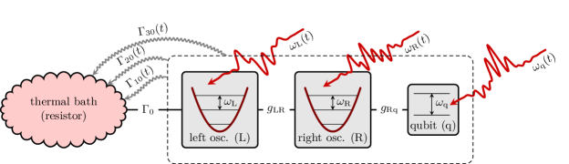
Figure 1: Schematic diagram of the considered physical scenario consisting of a qubit (q) linearly coupled to a harmonic oscillator (R), which in turn is linearly coupled to a second harmonic oscillator (L) that is in direct contact with a thermal bath. By temporally controlling the level splittings $\omega_{\mathrm{q/L/R}}(t)$ of the qubit, the right and the left oscillator, one can effectively tune the coupling strength to the bath and change the decay rates over several orders of magnitude.

II.1 Model

We consider a three-partite system consisting of two harmonic oscillators, named left (subscript L) and right (subscript R) oscillator, and a qubit (subscript q) as sketched in Fig. 1 and previously discussed in Refs. Partanen et al. (2018); Tuorila et al. (2017). We assume the two oscillators to be linearly coupled to each other through quadrature operators and the qubit to be exclusively coupled to the right oscillator. This scenario is modeled by the Hamiltonian (using units in which $\hbar=1$)

$$\mathsf{\hat{H}}(t) =\omega_{\mathrm{L}}(t)\mathsf{\hat{a}}_{\mathrm{L}}^{\dagger}\mathsf{\hat{a}}_{\mathrm{L}}+\omega_{\mathrm{R}}(t)\mathsf{\hat{a}}_{\mathrm{R}}^{\dagger}\mathsf{\hat{a}}_{\mathrm{R}}+\omega_{\mathrm{q}}(t)\mathsf{\hat{\sigma}}_{+}\mathsf{\hat{\sigma}}_{-}$$ (1)

$$\quad+g_{\mathrm{LR}}(t)\left(\mathsf{\hat{a}}_{\mathrm{L}}^{\dagger}+\mathsf{\hat{a}}_{\mathrm{L}}\right)\left(\mathsf{\hat{a}}_{\mathrm{R}}^{\dagger}+\mathsf{\hat{a}}_{\mathrm{R}}\right)$$

$$\quad-\textup{i}g_{\mathrm{Rq}}(t)\left(\mathsf{\hat{a}}_{\mathrm{R}}^{\dagger}+\mathsf{\hat{a}}_{\mathrm{R}}\right)\left(\mathsf{\hat{\sigma}}_{+}-\mathsf{\hat{\sigma}}_{-}\right),$$

where $\mathsf{\hat{a}}^{\dagger}_{\mathrm{L}}$, $\mathsf{\hat{a}}^{\dagger}_{\mathrm{R}}$ and $\mathsf{\hat{\sigma}}_{+}$ are the creation operators for the left oscillator, right oscillator and qubit, respectively. The first three terms in Eq. (1) describe the free evolution of the subsystems, with $\omega_{\mathrm{q}/\mathrm{L}/\mathrm{R}}(t)$ being the time-dependent and controllable level splittings of the qubit, the left and the right oscillator, respectively. The fourth and fifth term describe how the right oscillator is bi-linearly coupled to left oscillator and to the qubit with time-dependent interaction strengths $g_{\mathrm{LR}}(t)$ and $g_{\mathrm{Rq}}(t)$, respectively.

The Hamiltonian (1) can be simplified by applying a rotating-wave approximation, assuming $g_{\mathrm{Rq}}<g_{\mathrm{LR}}^{0}\ll\omega_{\mathrm{R}}$, where $g_{\mathrm{LR}}^{0}$ is the resonant coupling strength between the oscillators. This results in Tuorila et al. (2017)

$$\mathsf{\hat{H}}(t) \simeq\omega_{\mathrm{L}}(t)\mathsf{\hat{a}}_{\mathrm{L}}^{\dagger}\mathsf{\hat{a}}_{\mathrm{L}}+\omega_{\mathrm{R}}(t)\mathsf{\hat{a}}_{\mathrm{R}}^{\dagger}\mathsf{\hat{a}}_{\mathrm{R}}+\omega_{\mathrm{q}}(t)\mathsf{\hat{\sigma}}_{+}\mathsf{\hat{\sigma}}_{-}$$ (2)

$$\quad+g_{\mathrm{LR}}(t)\left(\mathsf{\hat{a}}_{\mathrm{L}}^{\dagger}\mathsf{\hat{a}}_{\mathrm{R}}+\mathsf{\hat{a}}_{\mathrm{R}}^{\dagger}\mathsf{\hat{a}}_{\mathrm{L}}\right)$$

$$\quad+\textup{i}g_{\mathrm{Rq}}(t)\left(\mathsf{\hat{a}}_{\mathrm{R}}^{\dagger}\mathsf{\hat{\sigma}}_{-}-\mathsf{\hat{a}}_{\mathrm{R}}\mathsf{\hat{\sigma}}_{+}\right).$$

Within this approximation, the number of excitations is a conserved quantity in the case of unitary evolution. Therefore, the total Hilbert space $\mathcal{H}$ of the system can be conveniently divided into subspaces $\mathcal{H}_{N}$ where the number of excitations $N$ is constant. A state belonging to a subspace $\mathcal{H}_{N}$ will thus remain within the subspace during the evolution that is solely governed by Hamiltonian (2).

However, we consider the three-partite system to be open, interacting with an environment through one of its subsystems. Specifically, we take the left oscillator to be linearly coupled to a thermal reservoir. Since we want this coupling to be relatively strong (compared to other typical relaxation rates), the right oscillator is needed as an intermediate component in order to allow efficient decoupling of the qubit from the reservoir. The system-bath interaction Hamiltonian is of the form Tuorila et al. (2017)

$$\mathsf{\hat{H}}_{\mathrm{int}}=\alpha\left(\mathsf{\hat{a}}_{\mathrm{L}}^{\dagger}+\mathsf{\hat{a}}_{\mathrm{L}}\right)\mathsf{\hat{V}}_{\mathrm{R}},$$ (3)

where $\mathsf{\hat{V}}_{\mathrm{R}}$ is an operator of the reservoir and $\alpha$ plays the role of an effective coupling strength. In order to derive a master equation for the open system, we employ its instantaneous eigenbasis $\{\ket{\Psi_{n}(t)}\}$, defined by $\mathsf{\hat{H}}(t)\ket{\Psi_{n}(t)}=\omega_{n}(t)\ket{\Psi_{n}(t)}$, with $\omega_{n}(t)$ being the respective eigenvalue. In this representation, the system-bath interaction can be rewritten as

$$\mathsf{\hat{H}}_{\mathrm{int}}=\alpha\sum_{m,n}v_{mn}\ket{\Psi_{m}(t)}\bra{\Psi_{n}(t)}\mathsf{\hat{V}}_{\mathrm{R}},$$ (4)

where

$$v_{mn}(t)=\bra{\Psi_{m}(t)}(\mathsf{\hat{a}}_{\mathrm{L}}^{\dagger}+\mathsf{\hat{a}}_{\mathrm{L}})\ket{\Psi_{n}(t)}.$$ (5)

Using standard techniques based on a weak-coupling hypothesis and the Born, Markov and secular approximations Breuer and Petruccione (2002), it is possible to derive a Markovian master equation for the open system. The decay rates, responsible for dissipation and decoherence, are given by

$$\Gamma_{mn}(t)=\alpha^{2}|v_{mn}(t)|^{2}S_{\mathrm{R}}\big{[}\omega_{mn}\left(t\right)\big{]},$$ (6)

where $\omega_{mn}(t)=\omega_{m}(t)-\omega_{n}(t)$ and $S_{\mathrm{R}}(\omega)$ is the real part of the Fourier transform of the reservoir correlation function,

$$S_{\mathrm{R}}(\omega)=\int_{-\infty}^{+\infty}\mathrm{d}s\,e^{\textup{i}\omega s}\Braket{\mathsf{\hat{V}}_{\mathrm{R}}(s)\mathsf{\hat{V}}_{\mathrm{R}}(0)}_{\mathrm{R}},$$ (7)

where the average $\braket{\dots}_{\mathrm{R}}$ is taken over the thermal state of the reservoir and the operators are expressed in the interaction picture with respect to the bath Hamiltonian. The corresponding master equation in the Lindblad form reads

$$\frac{\mathrm{d}}{\mathrm{d}t}\mathsf{\hat{\rho}}(t) =-\textup{i}\left[\mathsf{\hat{H}}(t),\mathsf{\hat{\rho}}(t)\right]$$

$$\quad+\sum_{m,n}\Gamma_{mn}(t)\Big{(}\mathsf{\hat{L}}_{mn}(t)\mathsf{\hat{\rho}}(t)\mathsf{\hat{L}}_{mn}^{\dagger}(t)$$

$$\qquad\qquad\qquad\quad-\frac{1}{2}\big{\{}\mathsf{\hat{L}}_{mn}^{\dagger}(t)\mathsf{\hat{L}}_{mn}(t),\mathsf{\hat{\rho}}(t)\big{\}}\Big{)},$$ (8)

where the Lindblad operators $\mathsf{\hat{L}}_{mn}(t)=\ket{\Psi_{m}(t)}\Bra{\Psi_{n}(t)}$ describe transitions among the eigenstates. A derivation of the master equation can be found in Appendix A. The Hamiltonian $\mathsf{\hat{H}}(t)$ can be directly controlled by tuning the level splittings $\omega_{\mathrm{q/L/R}}(t)$. Importantly, the Lindblad operators and decay rates inherit the temporal dependence from the instantaneous eigenstates and eigenvalues. As a consequence, Eq. (II.1) goes beyond the description based on static decay channels with constant rates, although we have neglected the correlations arising from the interplay between the temporal dependence of the Hamiltonian and the dissipation.

Solving the full master equation (II.1) is a rather challenging task and we therefore limit our study to a finite number of subspaces $\mathcal{H}_{N}$. Specifically, we consider the dynamics of the open system in the two subspaces $\mathcal{H}_{0}$ and $\mathcal{H}_{1}$, i.e., the subspace with no excitations, $\mathcal{H}_{0}=\mathrm{span}\{\ket{0,0,g}\}$, and that with a single excitation, $\mathcal{H}_{1}=\mathrm{span}\{\ket{0,0,e},\ket{0,1,g},\ket{1,0,g}\}$ where $\ket{0,0,g}=\ket{0}_{\mathrm{L}}\otimes\ket{0}_{\mathrm{R}}\otimes\ket{g}_{\mathrm{q}}$, $\ket{0,0,e}=\ket{0}_{\mathrm{L}}\otimes\ket{0}_{\mathrm{R}}\otimes\ket{e}_{\mathrm{q}}$, $\ket{0,1,g}=\ket{0}_{\mathrm{L}}\otimes\ket{1}_{\mathrm{R}}\otimes\ket{g}_{\mathrm{q}}$, $\ket{1,0,g}=\ket{1}_{\mathrm{L}}\otimes\ket{0}_{\mathrm{R}}\otimes\ket{g}_{\mathrm{q}}$. In the restricted Hilbert space, the Hamiltonian reads

$$H(t)=\begin{pmatrix}0&0&0&0\\ 0&\omega_{\mathrm{q}}(t)&-\textup{i}g_{\mathrm{Rq}}(t)&0\\ 0&\textup{i}g_{\mathrm{Rq}}(t)&\omega_{\mathrm{R}}(t)&g_{\mathrm{LR}}(t)\\ 0&0&g_{\mathrm{LR}}(t)&\omega_{\mathrm{L}}(t)\end{pmatrix}$$ (9)

in the basis $\{\ket{0,0,g},\ket{0,0,e},\ket{0,1,g},\ket{1,0,g}\}$. This simplified model can be solved analytically in the basis of the instantaneous eigenstates $\ket{\Psi_{1}(t)},\ket{\Psi_{2}(t)},\ket{\Psi_{3}(t)}\in\mathcal{H}_{1}$ and the ground state $\ket{\Psi_{0}}=\ket{0,0,g}$.

Accounting exclusively for population decay from the excited states in $\mathcal{H}_{1}$ to the ground state $\ket{0,0,g}$, but not for the reverse process of thermal excitation , we obtain the following Lindblad master equation, cf. Eq. (II.1),

$$\frac{\mathrm{d}}{\mathrm{d}t}\mathsf{\hat{\rho}}(t) =\mathcal{L}(t)\left[\mathsf{\hat{\rho}}(t)\right]=-\textup{i}\left[\mathsf{\hat{H}}(t),\mathsf{\hat{\rho}}(t)\right]+\mathcal{L}_{D}(t)\left[\mathsf{\hat{\rho}}(t)\right]$$ (10)

where

$$\mathcal{L}_{D}(t)\left[\mathsf{\hat{\rho}}(t)\right] =\sum_{i=1}^{3}\Gamma_{i0}(t)\Big{(}\mathsf{\hat{L}}_{i}(t)\mathsf{\hat{\rho}}(t)\mathsf{\hat{L}}_{i}^{\dagger}(t)$$

$$\qquad\qquad\qquad-\frac{1}{2}\big{\{}\mathsf{\hat{L}}_{i}^{\dagger}(t)\mathsf{\hat{L}}_{i}(t),\mathsf{\hat{\rho}}(t)\big{\}}\Big{)}$$ (11)

and the three time-dependent Lindblad operators are given by

$$\mathsf{\hat{L}}_{i}(t)=\ket{\Psi_{0}}\Bra{\Psi_{i}(t)},\qquad i=1,2,3.$$ (12)

Closed form expressions for the exact eigenvalues $\omega_{i}(t)$ and eigenstates $\ket{\Psi_{i}(t)}$, albeit rather lengthy, are straightforward to calculate with computer algebra.

Note that in addition to the tunable, engineered environment created by the left oscillator and the resistor, there exists in general also uncontrollable environments giving rise to the usual background lifetimes. Since the optimization scheme is essentially independent of such weak background coupling, we do not consider it further in this work.

II.2 Physical realization

The model introduced above is quite general. In the following, we focus on a possible experimental realization which implies certain constraints and specific functional dependencies between the bare frequencies of the three subsystems, $\{\omega_{\mathrm{L}}(t),\omega_{\mathrm{R}}(t),\omega_{\mathrm{q}}(t)\}$, and their respective couplings. The model described by Hamiltonian (1) can be realized by means of a superconducting qubit coupled to two $LC$ resonators Tuorila et al. (2017). The resonators behave effectively as quantum harmonic oscillators, the tunable frequencies of which are determined by the capacitance $C$ and a controllable inductance $L$, i.e., $\omega_{L/R}(t)=1/\sqrt{L_{L/R}(t)C_{L/R}}$. In this implementation, the couplings between the components can be expressed as functions of the physical parameters of the system and the bare resonator frequencies Tuorila et al. (2017).

The reservoir is realized by connecting a resistor to the left resonator with $\mathsf{\hat{V}}_{\mathrm{R}}$ in the interaction Hamiltonian (3) describing voltage fluctuations over the resistor. The resistor can be modeled as a thermal bath of bosonic modes Clerk et al. (2010), with the bath correlation function (7) corresponding to the Johnson-Nyquist spectrum,

$$S_{\mathrm{R}}(\omega)=\frac{2R\omega}{1-e^{-\omega/k_{\mathrm{B}}T_{\mathrm{env}}}},$$ (13)

where $R$ is the resistance of the resistor and $T_{\mathrm{env}}$ denotes its electron temperature Clerk et al. (2010). At low temperature, the spectral function (13) strongly suppresses emission of thermal excitations from the resistor so that indeed the population decay is the leading-order dissipative process for the studied three-partite quantum system. The decay rates can be expressed as Tuorila et al. (2017)

$$\Gamma_{i0}(t) =\Gamma_{0}\left|\Braket{\Psi_{0}(t)}{\mathsf{\hat{a}}_{\mathrm{L}}^{\dagger}+\mathsf{\hat{a}}_{\mathrm{L}}}{\Psi_{i}(t)}\right|^{2}$$

$$\quad\times\frac{\omega_{\mathrm{L}}(t)\omega_{i}(t)}{\omega_{\mathrm{R}}(t)^{2}}\frac{1}{1-e^{-\omega_{i}(t)/k_{\mathrm{B}}T_{\mathrm{env}}}},$$ (14)

where $\Gamma_{0}$ plays the role of a static decay rate. Note that the decay rates fulfill the detailed balance condition Tuorila et al. (2017)

$$\Gamma_{mn}(t)=\mathrm{exp}\left\{-\frac{\omega_{mn}(t)}{k_{\mathrm{B}}T_{\mathrm{env}}}\right\}\Gamma_{nm}(t),$$ (15)

which implies suppression of thermal excitations at low temperatures.

II.3 Quantum Optimal Control Theory

In general, QOCT aims at finding the optimal external control fields to steer the dynamics of a quantum system in the desired way Glaser et al. (2015). The starting point is to express the optimization task as a functional of the yet unknown external control fields $\{\mathcal{E}_{k}(t)\}$,

$$J\left[\left\{\mathcal{E}_{k}\right\}\right] =\alpha_{\tau}\left[\left\{\mathsf{\hat{\rho}}_{l}(\tau)\right\}\right]$$ (16)

$$\quad+\int_{0}^{\tau}\mathrm{d}t\,g\left[\left\{\mathcal{E}_{k}(t)\right\},\left\{\mathsf{\hat{\rho}}_{l}(t)\right\},t\right]\,.$$

Here, $\alpha_{\tau}$ denotes the final-time target functional which describes the actual optimization task such as the preparation of a specific target state. It may depend on one or several states $\mathsf{\hat{\rho}}_{l}(\tau)$, where the subscript $l$ denotes the different initial conditions of the temporal evolution. Furthermore, $g$ describes constraints that are relevant also at intermediate times, such as constraints on the intensity or spectrum of the yet unknown control fields Palao et al. (2013); Reich et al. (2014). A proper choice of the functional requires that the extremum is attained if and only if the task is carried out in an optimal way. In the example of state preparation, this is the case if the system state matches the desired target state perfectly. In the following, we discuss the two terms in the optimization functional (16) in more detail.

The final-time functional $\alpha_{T}$ measures how well the target is reached. For the reset task at hand, we seek to prepare the qubit in its ground state, irrespective of the initial state of the total system. This can be achieved by considering the dynamics for several initial states $\{\mathsf{\hat{\rho}}_{l}(t=0)\}$, making sure that all of them result in the desired target state Reich and Koch (2013). Moreover, no excitation should be left in any of the two oscillators, since otherwise these might get transferred to the qubit in an uncontrolled fashion later on. Hence, our set of initial states $\{\mathsf{\hat{\rho}}_{l}(t=0)\}$, is given by any complete basis of the excited subspace $\mathcal{H}_{1}$. The respective target state is the ground state of the total system $\mathsf{\hat{\rho}}_{\mathrm{trg}}=\ket{\Psi_{0}}\bra{\Psi_{0}}$. The final-time functional reads

$$\alpha_{\tau}=1-\frac{1}{3}\sum_{l=1}^{3}\left\langle\mathsf{\hat{\rho}}_{\mathrm{trg}},\mathcal{D}(\tau,0;\{\mathcal{E}_{k}\})\mathsf{\hat{\rho}}_{l}\right\rangle,$$ (17)

where $\langle\mathsf{\hat{A}},\mathsf{\hat{B}}\rangle=\mathrm{Tr}\{\mathsf{\hat{A}}^{\dagger}\mathsf{\hat{B}}\}$ and $\mathcal{D}(\tau,0;\{\mathcal{E}_{k}\})$ is the control-dependent dynamical map. Since $\alpha_{\tau}$ measures the remaining population in $\mathcal{H}_{1}$ at final time $\tau$, it corresponds to the error of the reset protocol. An ideal protocol is given by $\alpha_{\tau}=0$, which can be attained if and only if no population is left in $\mathcal{H}_{1}$. The final-time functional $\alpha_{\tau}$ provides a measure for how far the final state of the system is away from the desired target. It does not contain any information about the dynamics that brought it there.

Although our aim is to minimize Eq. (17), which quantifies the reset error, we will achieve this by minimization of the total functional (16). To this end, we employ Krotov’s method Krotov (1995); Konnov and Krotov (1999), an iterative optimization algorithm that comes with the advantage of monotonic convergence. Note that in Krotov’s method, the function $g$ is needed even if we do not want to impose constraints on the control fields or the system dynamics. In particular, the choice of $g$ determines the update rule for the control fields $\{\mathcal{E}_{k}(t)\}$ Palao and Kosloff (2003); Reich et al. (2012). Given the final-time target, a choice of $g$ in Eq. (16), and the equation of motion for the system, Eq. (10), Krotov’s method provides a recipe to derive an optimization algorithm to determine $\mathcal{E}_{k}$ Reich et al. (2012). Here, we use the standard choice of minimal amplitude increase per iteration step Palao and Kosloff (2003),

$$g\left[\left\{\mathcal{E}_{k}(t)\right\}\right]=\sum_{k}\frac{\lambda_{k}}{S_{k}(t)}\bigg{[}\mathcal{E}_{k}(t)-\mathcal{E}_{k}^{\mathrm{ref}}(t)\bigg{]}^{2},$$ (18)

where $\mathcal{E}_{k}^{\mathrm{ref}}(t)$ is a reference field for each $\mathcal{E}_{k}(t)$, taken to be the field from the previous iteration, $S_{k}(t)\in(0,1]$ a shape function to smoothly switch the field modulations on and off, and $\lambda_{k}$ a parameter that controls the update magnitude of $\mathcal{E}_{k}(t)$ in each optimization step. Due to the choice of $\mathcal{E}_{k}^{\mathrm{ref}}(t)$ to be the control field from the last iteration, the difference $\mathcal{E}_{k}(t)-\mathcal{E}_{k}^{\mathrm{ref}}(t)$ approaches zero as the optimization converges. Hence, the contribution of $g$ to the total functional (16) decreases as well. As the optimum is approached, the value of the overall functional (16) is essentially given by the value of $\alpha_{\tau}$ as desired.

With Eq. (18), the update equation for $\mathcal{E}_{k}(t)$ reads Reich et al. (2012)

$$\mathcal{E}_{k}^{(i+1)}(t)=\mathcal{E}_{k}^{(i)}(t)+\frac{S_{k}(t)}{\lambda_{k}}\mathfrak{Im}\left\{\sum_{l}\Braket{\mathsf{\hat{\chi}}^{(i)}_{l}(t)\;,\;\frac{\partial\mathcal{L}\left[\left\{\mathcal{E}_{k^{\prime}}\right\}\right]}{\partial\mathcal{E}_{k}}\Big{missing}}{{}_{\{\mathcal{E}^{(i+1)}_{k^{\prime}}(t)\}}\mathsf{\hat{\rho}}^{(i+1)}_{l}(t)}\right\},$$ (19)

where $\{\mathsf{\hat{\rho}}^{(i+1)}_{l}(t)\}$ are the forward propagated initial states spanning $\mathcal{H}_{1}$, obtained by solving

$$\frac{\mathrm{d}}{\mathrm{d}t}\mathsf{\hat{\rho}}^{(i+1)}_{l}(t)=-\textup{i}\mathcal{L}\left[\left\{\mathcal{E}^{(i+1)}_{k}\right\}\right]\mathsf{\hat{\rho}}^{(i+1)}_{l}(t)\,.$$ (20)

The so-called co-states $\{\mathsf{\hat{\chi}}^{(i)}_{l}(t)\}$ in Eq. (19) are solutions of the adjoint equation of motion,

$$\frac{\mathrm{d}}{\mathrm{d}t}\mathsf{\hat{\chi}}^{(i)}_{l}(t)=\textup{i}\mathcal{L}^{\dagger}\left[\left\{\mathcal{E}^{(i)}_{k}\right\}\right]\mathsf{\hat{\chi}}^{(i)}_{l}(t)\,,$$ (21)

with boundary condition $\mathsf{\hat{\chi}}^{(i)}_{l}(\tau)=-\nabla_{\mathsf{\hat{\rho}}_{l}(\tau)}\alpha_{\tau}\big{|}_{\{\mathsf{\hat{\rho}}^{(i)}_{l^{\prime}}(\tau)\}}$. The derivative of $\alpha_{\tau}$ with respect to $\mathsf{\hat{\rho}}_{l}(\tau)$ can be turned into a usual gradient by representing the states in a complete, orthonormal basis Palao and Kosloff (2003). Note that the indices $(i+1)$ and $(i)$ indicate values for current and last iteration, respectively.

As with any optimization algorithm based on variational calculus, Krotov’s method requires the calculation of gradients—one of them the gradient of the dynamical generator with respect to the controls, cf. Eq. (19). Peculiarly, not just the Hamiltonian $\mathsf{\hat{H}}$, cf. Eq. (9), but also the dissipator $\mathcal{L}_{D}$, cf. Eq. (II.1) depends on the controls and thus contributes to the gradient,

$$\frac{\partial\mathcal{L}\left[\left\{\mathcal{E}_{k^{\prime}}\right\}\right]}{\partial\mathcal{E}_{k}}\mathsf{\hat{\rho}}=-\textup{i}\left[\frac{\partial\mathsf{\hat{H}}\left[\left\{\mathcal{E}_{k^{\prime}}\right\}\right]}{\partial\mathcal{E}_{k}},\mathsf{\hat{\rho}}\right]+\frac{\partial\mathcal{L}_{D}\left[\left\{\mathcal{E}_{k^{\prime}}\right\}\right]}{\partial\mathcal{E}_{k}}\mathsf{\hat{\rho}}.$$ (22)

Whereas the gradient of the Hamiltonian with respect to $\omega_{\mathrm{L}}$, $\omega_{\mathrm{R}}$ and $\omega_{\mathrm{q}}$ is straightforward to calculate, cf. Eq. (9), the gradient of the dissipator $\mathcal{L}_{D}$ is rather lengthy to evaluate, cf. Eq. (II.1). This inconvenience is due to the dependence of the decay rates $\Gamma_{i0}$ and Lindblad operators $\mathsf{\hat{L}}_{i}$ on the instantaneous eigenvalues $\omega_{i}(t)$ and eigenstates $\ket{\psi_{i}(t)}$. The required derivatives of $\omega_{i}(t)$ and $\ket{\psi_{i}(t)}$ with respect to $\omega_{\mathrm{L}}$, $\omega_{\mathrm{R}}$, and $\omega_{\mathrm{q}}$ have been algebraically calculated using computer software.

III Numerical Results

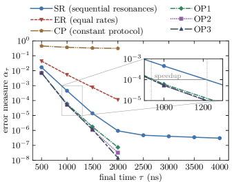
Figure 2: Excited state population $\alpha_{\tau}$, Eq. (17), as a function of protocol length $\tau$ for different control fields. SR denotes the original protocol utilizing sequential resonances with the resistive bath Tuorila et al. (2017), CP refers to a protocol with only constant fields, and OP1, OP2, and OP3 are results obtained with SR or CP as guess control fields to start the optimization (see main text for detailed explanations). An optimization targeting equal dissipation rates, cf. Eq. (25), instead of minimizing $\alpha_{\tau}$ is labeled by ER. The inset highlights the speedup due to the optimization, by comparing the durations for which the optimized protocols and the SR reach an error of $10^{-4}$. The parameters are summarized in Table 1.

Table 1: Parameters used in the calculations for the setup shown in Fig. (1). The parameters are taken from Ref. Tuorila et al. (2017) and correspond to an experimentally feasible circuit QED realization. Here, $T_{\mathrm{env}}$ is a typical temperature for dilution refrigerators used to operate superconducting qubits Gambetta et al. (2017).

left oscillator frequency	$\omega_{\mathrm{L}_{0}}/2\pi$	$11.5$ GHz
right oscillator frequency	$\omega_{\mathrm{R}}/2\pi$	$10.0$ GHz
qubit frequency	$\omega_{\mathrm{q}}/2\pi$	$9.5$ GHz
right osc.-qubit coupling	$g_{\mathrm{Rq}}/2\pi$	$68$ MHz
left-right osc. coupling	$g_{\mathrm{LR}_{0}}/2\pi$	$74$ MHz
static decay rate	$\Gamma_{0}$	$31$ MHz
temperature	$T_{\mathrm{env}}$	$10$ mK

III.1 Optimization of the original protocol

The original protocol Tuorila et al. (2017) is based on a simple choice for the left-oscillator frequency $\omega_{\mathrm{L}}(t)$. Effectively, it consists of two stages, namely $\omega_{\mathrm{L}}(t)=\omega_{+}$ and $\omega_{\mathrm{L}}(t)=\omega_{-}$, separated by an intermediate ramp. The entire protocol reads

$$\omega_{\mathrm{L}}(t)=\left\{\begin{aligned} &\omega_{\mathrm{L}_{0}}\rightarrow\omega_{+},&&\qquad 0&&\leq t<t_{\mathrm{R}};\\ &\omega_{+},&&\qquad t_{\mathrm{R}}&&\leq t<\tau/2;\\ &\omega_{+}\rightarrow\omega_{-},&&\qquad\tau/2&&\leq t<\tau/2+t_{\mathrm{R}};\\ &\omega_{-},&&\qquad\tau/2+t_{\mathrm{R}}&&\leq t<\tau-t_{\mathrm{R}};\\ &\omega_{-}\rightarrow\omega_{\mathrm{L}_{0}},&&\qquad\tau-t_{\mathrm{R}}&&\leq t\leq\tau;\end{aligned}\right.$$ (23)

where $\tau$ is the total protocol duration, $\tau/2$ is the hold time at each stage, and $t_{\mathrm{R}}\ll\tau$ is the ramping duration. The ramp formula has been chosen to be

$$\omega_{\mathrm{L}}(t)=\omega_{0}+\left(\omega_{1}-\omega_{0}\right)f\left(\frac{t-t_{0}}{t_{1}-t_{0}}\right)$$ (24)

with $f(x)=6x^{5}-15x^{4}+10x^{3}$, which ramps $\omega_{\mathrm{L}}(t)$ smoothly from $\omega_{0}$ to $\omega_{1}$ as time goes from $t_{0}$ to $t_{1}$. The operation points $\omega_{+}$ and $\omega_{-}$ have been chosen such that $\Gamma_{20}(t)=\Gamma_{30}(t)$ in the case of $\omega_{+}$ and $\Gamma_{10}(t)=\Gamma_{20}(t)$ for $\omega_{-}$. This choice guarantees that any excitation decays at some point of time during the protocol.

Figure 2 illustrates the performance of the protocol of sequential resonances (SR) with the resistive bath as a function of its duration $\tau$. It shows a rapid approach towards errors $\alpha_{\tau}$ as small as $10^{-6}$ for $\tau=$2000\text{\,}\mathrm{ns}$$ for the parameters listed in Table 1. Although this may be sufficient for some applications, the SR exhibits a plateau for longer durations, preventing it even theoretically to reach significantly smaller errors. The plateau is caused by population being locked in the excited state of the right oscillator — an unfavorable feature that is apparently not resolvable by simply extending the protocol duration. However, taking Eq. (23) as the initial guess for the above described optimization procedure, Fig. 2 shows that, depending on $\tau$, an improvement of up to two orders of magnitude in the error $\alpha_{\tau}$ compared to the SR is possible. In addition, this optimized protocol (OP1) also resolves the issue of the plateau, reaching errors $\alpha_{\tau}<10^{-7}$. The improvement with respect to the protocol duration is comparatively modest, as the inset of Fig. 2 illustrates. Taking, e.g., $\alpha_{\tau}=10^{-4}$ as a sufficiently small error, the speedup with respect to the SR is roughly $\Delta\tau\approx$280\text{\,}\mathrm{ns}$$.

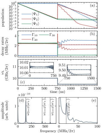
Figure 3: Dynamics for the SR (dashed lines) and its optimized version OP1 (solid lines) for a protocol duration of $\tau=$1500\text{\,}\mathrm{ns}$$, cf. Fig. 2. Note that dashed lines partly overlap. (a) Population in the three eigenstates of the excited subspace $\mathcal{H}_{1}$. (b) Decay rates, cf. Eq. (II.2), from $\mathcal{H}_{1}$ into the total ground state $\ket{\Psi_{0}}$. (c) Left oscillator frequency $\omega_{\mathrm{L}}(t)$ following the original two stage protocol of Eq. (23). The two stages are still visible in the optimized version, with modulations on top, as highlighted by the two insets. The shaded area in the left inset corresponds to fast oscillations, which are not resolved due to the linewidth. (d) and (e) show the frequency spectra of the optimized splitting $\omega_{\mathrm{L}}(t)$ from the left and right insets of (c), respectively. The vertical lines indicate frequency differences, $\omega_{i\leftrightarrow j}=\left|\omega_{i}-\omega_{j}\right|$ with $\omega_{i}=\omega_{i}(\omega_{\mathrm{L}})$ being the instantaneous eigenvalues.

Figure 3 compares the decay dynamics of SR and OP1, for $\tau=$1500\text{\,}\mathrm{ns}$$, showing the population of the excited eigenstates in Figs. 3(a) and the respective decay rates and control fields $\omega_{\mathrm{L}}(t)$ generating them in Fig. 3(b) and 3(c). We observe that the original two-stage protocol (SR) acts as intended, i.e., the population decays from all three eigenstates of $\mathcal{H}_{1}$. Since the intermediate ramp transfers a significant amount of population from $\ket{\Psi_{1}}$ to $\ket{\Psi_{2}}$, $\Gamma_{20}(t)$ needs to be sufficiently large also during the second stage. Note that this population transfer between different eigenstates within $\mathcal{H}_{1}$ occurs due to non-adiabatic transitions caused by changes of those particular eigenstates . These are caused by changes in the control function $\omega_{\mathrm{L}}(t)$, i.e., the ramps in the SR.

A similar reasoning readily explains also the behavior of the control field in case of OP1, shown in Fig. 3(c). Compared to the SR, the optimization effectively shifts the base levels of $\omega_{\mathrm{L}}$ at both stages and adds oscillations on top. This results in an increase of $\Gamma_{10}(t)$ and a decrease of $\Gamma_{20}(t)$, cf. Fig. 3(b), in particular during the second stage, directly causing the population of $\ket{\Psi_{1}(t)}$ ($\ket{\Psi_{2}(t)}$) to decay faster (slower). The additional oscillations, even though having small amplitude, drive non-adiabatic transitions between $\ket{\Psi_{1}}$ and $\ket{\Psi_{2}}$, which primarily transfer population to the fast decaying state $\ket{\Psi_{1}}$, cf. Fig. 3(a). This becomes even more clear by inspecting Figs. 3(d) and 3(e), which show the spectra corresponding to the insets of Fig. 3(c). In both cases, the frequencies match the differences between various eigenvalues $\omega_{i}$, evaluated at $\omega_{+}$ and $\omega_{-}$ for $\omega_{\mathrm{L}}$ in the left and right inset, respectively. Whereas the spectrum shown in Fig. 3(d) is dominated by a peak at $\omega_{2\leftrightarrow 3}$, which does not seem to have a notable impact on the dynamics, Fig. 3(e) exhibits a peak at $\omega_{1\leftrightarrow 2}$ and is responsible for the above-mentioned population transfer between $\ket{\Psi_{1}}$ and $\ket{\Psi_{2}}$. The combination of increasing decay rates and engineered population transfer results in the excitation to more efficiently decay from both states. The required control of the left oscillator frequency $\omega_{\mathrm{L}}(t)$ can, for instance, be achieved by Josephson parametric amplifiers Yamamoto et al. (2008).

The optimization studied in Fig. 3 changes the coherent part of the evolution compared to the SR, creating non-adiabatic transitions by suitably modulating $\omega_{\mathrm{L}}(t)$ and adapting the decay rates $\Gamma_{i0}(t)$ accordingly. Both effects are necessary to explain the observed improvement with respect to the SR. In contrast, Fig. 2 shows also optimization results where the system dynamics has been completely ignored in the optimization process. In this case, the minimization of Eq. (16) has been replaced by a functional targeting equal dissipation rates (ER). Namely, we have optimized $\omega_{\mathrm{L}}(t)$ to yield $R_{1}\approx R_{2}\approx R_{3}$ with each $R_{i}$ as large as possible, where

$$R_{i}=\int_{0}^{\tau}\Gamma_{i0}(t)\,\mathrm{d}t,\qquad i=1,2,3,$$ (25)

are the time-integrated dissipation rates which are independent of the system dynamics. The naive assumption behind this optimization is that, since all states $\mathsf{\hat{\rho}}_{1},\mathsf{\hat{\rho}}_{2},\mathsf{\hat{\rho}}_{3}$ are equally weighted in Eq. (17), equal dissipation from all of them may be a good choice to decrease the error $\alpha_{\tau}$. However, this is not the case, cf. Fig. 2, which emphasizes the interplay of coherent and dissipative dynamics in the problem at hand.

III.2 Optimization with an extended set of control fields

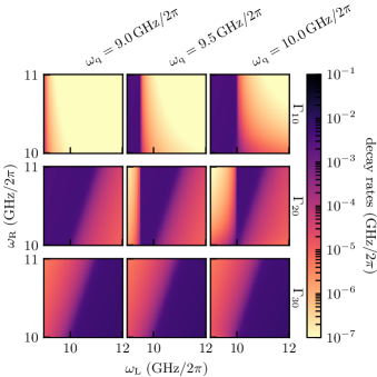
Figure 4: Decay rates $\Gamma_{i0}$ from the excited subspace $\mathcal{H}_{1}$ into the total ground state $\ket{\Psi_{0}}$, cf. Eq. (II.2), as a function of level splittings $\omega_{\mathrm{L}}$ and $\omega_{\mathrm{R}}$ and for three different values of $\omega_{\mathrm{q}}$.

In the following, we extend the SR by assuming the frequencies of the right oscillator and of the qubit, $\omega_{\mathrm{R}}(t)$ and $\omega_{\mathrm{q}}(t)$, to be temporally controllable. Since the eigenvalues $\omega_{i}(t)$ and eigenstates $\ket{\Psi_{i}(t)}$ ($i=1,2,3$) depend on all three frequencies, $\omega_{\mathrm{L}}$, $\omega_{\mathrm{R}}$ and $\omega_{\mathrm{q}}$, changing any of them may affect the dynamics. In other words, more control fields give the optimization more flexibility to steer the system dynamics in the desired way and engineer the dissipation rates more appropriately.

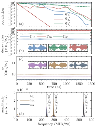
Figure 5: Dynamics obtained with the constant protocol CP (dashed lines) and its optimized version OP3 (solid lines). The panels are as in Fig. 3 with the small insets in (b) and (c) providing a closer look at the shapes of the optimized fields, respectively decay rates, compared to their non-optimized, constant counterparts. Panel (d) shows the spectra of all optimized fields from panel (c).

First, we inspect in Fig. 4 how the decay rates change as a function of the level splittings $\omega_{\mathrm{L}}$, $\omega_{\mathrm{R}}$, and $\omega_{\mathrm{q}}$. Two important observations can be made from Fig. 4. On one hand, the decay rates are still mutually exclusive, in the sense that there exists no combination such that two of them are maximal at the same time. On the other hand, the attainable total maximum of each individual decay rate as a function of all three controls $\omega_{\mathrm{L}}$, $\omega_{\mathrm{R}}$ and $\omega_{\mathrm{q}}$ does not change. Hence, adjusting $\omega_{\mathrm{R}}$ or $\omega_{\mathrm{q}}$ in addition to $\omega_{\mathrm{L}}$ does not yield essentially larger rates, and there will not be a significantly faster decay to the ground state. Although no naive improvement is to be expected from simply increasing the decay rates, i.e., due to the dissipative part of the dynamics, one may still achieve an improvement by more appropriately steering the coherent part.

Figure 2 shows optimization results for the case that all three frequencies are time-dependent (OP2). The initial guess has been chosen according to the SR, i.e., Eq. (23) for $\omega_{\mathrm{L}}(t)$ and constant values for $\omega_{\mathrm{R}}$, $\omega_{\mathrm{q}}$. Despite the extended set of controls, the optimization does not yield errors significantly below the case where only $\omega_{\mathrm{L}}(t)$ is controlled. This finding is reproducible even when using different sets of controls, such as only using $\omega_{\mathrm{q}}(t)$ and $\omega_{\mathrm{L}}$ or only using $\omega_{\mathrm{q}}(t)$ and $\omega_{\mathrm{R}}$ (data not shown). We therefore expect that further controls beyond $\omega_{\mathrm{L}}(t)$ do not allow the coherent part of the dynamics to be steered more efficiently.

In order to study this expectation further and evaluate the impact of the guess fields, we have carried out optimizations with all three possible controls. Whereas $\omega_{\mathrm{R}}$ and $\omega_{\mathrm{q}}$ have been set constant as initial guess, $\omega_{\mathrm{L}}(t)$ has been chosen as $\omega_{\mathrm{L}}(t)=(\omega_{+}+\omega_{-})/2$ with additional ramps in the beginning and end. Due to this choice, $\Gamma_{20}$ is almost maximal during the entire protocol, whereas $\Gamma_{10}$ and $\Gamma_{30}$ are orders of magnitude smaller, cf. Fig. 4. Thus, only population in $\ket{\Psi_{2}}$ decays fast. Simply extending the protocol duration $\tau$ will not solve the problem of small $\Gamma_{10}$ and $\Gamma_{30}$. Upon optimization, we are, however, able to find fields yielding similarly small errors $\alpha_{\tau}$ as before, cf. OP3 with OP1 and OP2 in Fig. 2. We again analyze an exemplary dynamics for $\tau=$1500\text{\,}\mathrm{ns}$$ in Fig. 5. Figure 5(a) shows the population dynamics. As expected, the population in $\ket{\Psi_{2}}$ decays rapidly under the constant guess fields, while $\ket{\Psi_{3}}$ exhibits only slow decay and the population in $\ket{\Psi_{1}}$ is almost conserved. The respective decay rates and control fields are shown in Figs. 5(b) and 5(c). Interestingly, the optimization leaves the base levels of each control field unchanged, again adding small oscillations on top. Consequently, the decay rates are unchanged in magnitude but exhibit small oscillations as well. Since $\Gamma_{20}$ is already maximal by choice of the guess fields, cf. Fig. 4, there is no possibility for the optimization to increase it. Instead, the optimization ensures that all excitations are coherently transferred to this strongly decaying state — in our example from $\ket{\Psi_{1}}$ and $\ket{\Psi_{3}}$ to $\ket{\Psi_{2}}$, as evident from Fig. 5(a). Thus, we find a similar reset strategy as in Fig. 3: The control fields are tailored such that a single decay rate (not necessarily the same at different times) is maximal and population is transferred coherently into this strongly decaying state.

We expect the reset strategies illustrated in Figs. 3 and 5 to be feasible for essentially any combination of control fields and choice of guess fields. This follows from the decay rates being mutually exclusive, cf. Fig. 4, i.e., if one state has a maximal decay rate, the other two states decay slower. All that is hence required is to ensure coherent population transfer into this state which seems to be possible by tailoring the control fields. Remarkably, the addition of further control fields does not result in significantly smaller errors $\alpha_{\tau}$, cf. Fig. 2. In fact, $\omega_{\mathrm{L}}(t)$ alone is already sufficient to fully control the decay rates and engineer the required population transfer. Nevertheless, adding more control options increases flexibility and is thus potentially beneficial in experiments, especially if certain control fields are convenient to implement experimentally.

IV Summary and Conclusions

In summary, we have studied how optimization of external control fields speeds up the initialization of a superconducting qubit which is tunably coupled to a thermal bath via two resonators. The control knobs are the time-dependent level splittings of the qubit and the resonators. Starting from a protocol utilizing sequential resonances with the resistive bath and employing the level splitting of a single resonator as the only control field, while assuming the initial state to be confined to the single excitation subspace Tuorila et al. (2017), we have replaced the analytically derived temporal dependence by a numerically optimized control field. This has allowed us to obtain an improvement in both the reset speed and fidelity.

We have also tested whether adding multiple control fields, by explicitly accounting for the tunability of the level splitting of the qubit and of the second resonator, results in additional improvements. This has turned out to not to be the case. Moreover, we have found that in all control scenarios, the optimized reset strategy consists in maximizing the decay rate from a single state and driving non-adiabatic population transfer into the strongly decaying state by small oscillations in the control fields. Even for different combinations of control fields and various guess fields, the optimization has resulted in reset errors and times of the same order of magnitude. We thus suspect to have identified the quantum speed limit for qubit reset in this particular physical setup with tunable couplings, provided that only a single excitation at maximum is present initially. However, a more rigorous study exploring the full parameter space is required to prove that our solution represents indeed a global, and not only a local, optimum.

Whether the quantum speed limit identified in our study is related to the rotating-wave or other used approximations remains an open question. In particular, it will be interesting to study whether the reset duration and error can be further decreased by utilizing couplings between the single-excitation subspace and higher-excitation subspaces. The rationale would be that highly excited states decay faster which might further decrease the protocol duration. The required transitions could again be driven by suitably shaped control fields determined by QOCT.

Our study is, to the best of our knowledge, the first demonstration of experimentally directly applicable reservoir engineering using quantum optimal control of time-dependent decay rates. It is related to earlier results obtained for controlling open quantum systems with non-Markovian dynamics which had shown, for example, improved cooling due to cooperative effects of control and dissipation Schmidt et al. (2011) or better gate operations Rebentrost et al. (2009); Reich et al. (2015). Our approach differs from the more common scenario for the control of open quantum systems in which the external field modifies only the Hamiltonian and thus the coherent part of the dynamics, rather than the dissipator of the master equation Koch (2016). In contrast, in our example, both the coherent evolution and the decay rates change in time as a result of the field optimization . Specifically, the changes in the coherent dynamics are manifested in the occurrence of non-adiabatic transitions which go hand in hand with modifications in the time-dependent decay rates. Interestingly, coherent and dissipative dynamics are tightly intertwined and the optimization protocol affects both in a physically transparent way. Our study thus paves the way to explore quantum reservoir engineering in condensed phase settings.

Appendix A Derivation of the Master Equation

In this appendix, we provide details on how to obtain the Lindblad master equation (II.1). It follows in large parts the derivation in Ref. Tuorila et al. (2017). We know that the combined dynamics of the system and the environment follows is unitary and obeys the von Neumann equation

$$\frac{\mathrm{d}}{\mathrm{d}t}\mathsf{\hat{\rho}}_{\mathrm{tot}}(t) =-\textup{i}\left[\mathsf{\hat{H}}_{\mathrm{tot}}(t),\mathsf{\hat{\rho}}_{\mathrm{tot}}(t)\right],$$ (26)

where $\mathsf{\hat{\rho}}_{\mathrm{tot}}(t)$ is the joint state of the system and the environment and

$$\mathsf{\hat{H}}_{\mathrm{tot}}(t)=\mathsf{\hat{H}}(t)+\mathsf{\hat{H}}_{\mathrm{env}}+\mathsf{\hat{H}}_{\mathrm{int}},$$ (27)

is the total Hamiltonian, $\mathsf{\hat{H}}_{\mathrm{env}}$ is the Hamiltonian of the environment alone and $\mathsf{\hat{H}}(t)$ and $\mathsf{\hat{H}}_{\mathrm{int}}$ are given by Eqs. (2) and (3), respectively. In order to obtain an equation of motion for the reduced dynamics of the system alone, i.e., $\mathsf{\hat{\rho}}(t)=\mathrm{tr}_{\mathrm{env}}\left\{\mathsf{\hat{\rho}}_{\mathrm{tot}}(t)\right\}$, we start with applying a unitary transformation $\mathsf{\hat{D}}(t)=\sum_{n}\Ket{\psi_{n}}\Bra{n}$ that diagonalizes $\mathsf{\hat{H}}(t)$, where $\{\ket{n}\}$ is a time-independent basis. In the new basis of eigenstates $\{\ket{\Psi_{n}(t)}\}$ of $\mathsf{\hat{H}}(t)$, the system Hamiltonian reads

$$\mathsf{\hat{H}}_{\mathrm{eff}}(t) =\sum_{n,m}\left[\omega_{n}(t)\delta_{n,m}-\textup{i}\Braket{\Psi_{n}(t)}{\dot{\Psi}_{m}(t)}\right]\ket{n}\bra{m},$$ (28)

where $\omega_{n}(t)$ is the corresponding eigenvalue of $\ket{\Psi_{n}(t)}$. The second term in Eq. (28) is responsible for non-adiabatic couplings between different eigenstates. The derivation of the master equation starts with conventional assumptions like initial separability, $\mathsf{\hat{\rho}}_{\mathrm{tot}}(0)=\mathsf{\hat{\rho}}(0)\otimes\mathsf{\hat{\rho}}_{\mathrm{env}}(0)$, a thermal and static state of the bath $\mathsf{\hat{\rho}}_{\mathrm{env}}(t)\approx\mathsf{\hat{\rho}}_{\mathrm{env}}(0)$, weak coupling between the system and its environment and the typical Born-Markov and secular approximations Breuer and Petruccione (2002). We obtain the general Lindblad master equation (II.1), where the decay rates $\Gamma_{mn}(t)$ are still undefined. However, it can be shown that the decay rates coincide with the ones that can be obtained with Fermi’s golden rule Alicki (1977). This yields the general expression in Eq. (6) for the decay rates. By substituting $v_{mn}(t)$ and $S_{\mathrm{R}}$ from Eqs. (5) and (13), respectively, one arrives at the decay rates in Eq. (II.2). Due to the form of the system-environment interaction (4), dephasing processed described by rates $\Gamma_{nn}(t)$ vanish. Moreover, since the detailed balance (15) holds and taking the temperature of the environment low, heating processes are strongly suppressed and cooling is the dominant source of dissipation.

Note that the frame, where the Hamiltonian $\mathsf{\hat{H}}(t)$ is diagonal, i.e., Eq. (28), is only used for the derivation of the decay rates. In the numerical simulations, all operators and states are still expressed in the static basis $\{\ket{0,0,g},\ket{0,0,e},\ket{0,1,g},\ket{1,0,g}\}$.

References

- Gambetta et al. (2017) J. M. Gambetta, J. M. Chow, and M. Steffen, npj Quantum Inf. 3, 2 (2017).
- Basilewitsch et al. (2017) D. Basilewitsch, R. Schmidt, D. Sugny, S. Maniscalco, and C. P. Koch, New J. Phys. 19, 113042 (2017).
- Magnard et al. (2018) P. Magnard, P. Kurpiers, B. Royer, T. Walter, J.-C. Besse, S. Gasparinetti, M. Pechal, J. Heinsoo, S. Storz, A. Blais, and A. Wallraff, Phys. Rev. Lett. 121, 060502 (2018).
- Rodríguez-Briones et al. (2017a) N. A. Rodríguez-Briones, E. Martín-Martínez, A. Kempf, and R. Laflamme, Phys. Rev. Lett. 119, 050502 (2017a).
- Rodríguez-Briones et al. (2017b) N. A. Rodríguez-Briones, J. Li, X. Peng, T. Mor, Y. Weinstein, and R. Laflamme, New J. Phys. 19, 113047 (2017b).
- Pierre et al. (2014) M. Pierre, I.-M. Svensson, S. Raman Sathyamoorthy, G. Johansson, and P. Delsing, Appl. Phys. Lett. 104, 232604 (2014).
- Tan et al. (2017) K. Y. Tan, M. Partanen, R. E. Lake, J. Govenius, S. Masuda, and M. Möttönen, Nature Commun. 8, 15189 (2017).
- Partanen et al. (2018) M. Partanen, K. Y. Tan, S. Masuda, J. Govenius, R. E. Lake, M. Jenei, L. Grönberg, J. Hassel, S. Simbierowicz, V. Vesterinen, J. Tuorila, T. Ala-Nissila, and M. Möttönen, Sci. Rep. 8, 6325 (2018).
- Silveri et al. (2019) M. Silveri, S. Masuda, V. Sevriuk, K. Y. Tan, M. Jenei, E. Hyyppä, F. Hassler, M. Partanen, J. Goetz, R. E. Lake, L. Grönberg, and M. Möttönen, Nature Phys. (2019).
- Wong et al. (2019) C. H. Wong, C. Wilen, R. McDermott, and M. G. Vavilov, Quantum Sci. Technol. 4, 025001 (2019).
- Tuorila et al. (2017) J. Tuorila, M. Partanen, T. Ala-Nissilä, and M. Möttönen, npj Quantum Inf. 3, 27 (2017).
- Glaser et al. (2015) S. J. Glaser, U. Boscain, T. Calarco, C. P. Koch, W. Köckenberger, R. Kosloff, I. Kuprov, B. Luy, S. Schirmer, T. Schulte-Herbrüggen, D. Sugny, and F. K. Wilhelm, Eur. Phys. J. D 69, 279 (2015).
- Suter and Álvarez (2016) D. Suter and G. A. Álvarez, Rev. Mod. Phys. 88, 041001 (2016).
- Caneva et al. (2011) T. Caneva, T. Calarco, and S. Montangero, Phys. Rev. A 84, 022326 (2011).
- Krotov (1995) V. Krotov, Global Methods in Optimal Control Theory (CRC Press, 1995).
- Khaneja et al. (2005) N. Khaneja, T. Reiss, C. Kehlet, T. Schulte-Herbrüggen, and S. J. Glaser, J. Mag. Res. 172, 296 (2005).
- Koch (2016) C. P. Koch, J. Phys.: Condens. Matter 28, 213001 (2016).
- Bartana et al. (1993) A. Bartana, R. Kosloff, and D. J. Tannor, J. Comp. Phys. 99, 196 (1993).
- Bartana et al. (1997) A. Bartana, R. Kosloff, and D. J. Tannor, J. Comp. Phys. 106, 1435 (1997).
- Schmidt et al. (2011) R. Schmidt, A. Negretti, J. Ankerhold, T. Calarco, and J. T. Stockburger, Phys. Rev. Lett. 107, 130404 (2011).
- Boutin et al. (2017) S. Boutin, C. K. Andersen, J. Venkatraman, A. J. Ferris, and A. Blais, Phys. Rev. A 96, 042315 (2017).
- Fischer et al. (2019) J. Fischer, D. Basilewitsch, C. P. Koch, and D. Sugny, Phys. Rev. A 99, 033410 (2019).
- Poyatos et al. (1996) J. F. Poyatos, J. I. Cirac, and P. Zoller, Phys. Rev. Lett. 77, 4728 (1996).
- Kraus et al. (2008) B. Kraus, H. P. Büchler, S. Diehl, A. Kantian, A. Micheli, and P. Zoller, Phys. Rev. A 78, 042307 (2008).
- Verstraete et al. (2009) F. Verstraete, M. M. Wolf, and J. I. Cirac, Nature Phys. 5, 633 (2009).
- Krauter et al. (2011) H. Krauter, C. A. Muschik, K. Jensen, W. Wasilewski, J. M. Petersen, J. I. Cirac, and E. S. Polzik, Phys. Rev. Lett. 107, 080503 (2011).
- Lin et al. (2013) Y. Lin, J. Gaebler, F. Reiter, T. Tan, R. Bowler, A. Sørensen, D. Leibfried, and D. Wineland, Nature 504, 415 (2013).
- Kienzler et al. (2014) D. Kienzler, H.-Y. Lo, B. Keitch, L. de Clercq, F. Leupold, F. Lindenfelser, M. Marinelli, V. Negnevitsky, and J. P. Home, Science 347, 53 (2014).
- Doucet et al. (2018) E. Doucet, F. Reiter, L. Ranzani, and A. Kamal, arXiv:1810.03631 (2018).
- Horn et al. (2018) K. P. Horn, F. Reiter, Y. Lin, D. Leibfried, and C. P. Koch, New J. Phys. 20, 123010 (2018).
- Paladino et al. (2014) E. Paladino, Y. M. Galperin, G. Falci, and B. L. Altshuler, Rev. Mod. Phys. 86, 361 (2014).
- Rebentrost et al. (2009) P. Rebentrost, I. Serban, T. Schulte-Herbrüggen, and F. K. Wilhelm, Phys. Rev. Lett. 102, 090401 (2009).
- Rivas et al. (2014) Á. Rivas, S. F. Huelga, and M. B. Plenio, Rep. Prog. Phys. 77, 094001 (2014).
- Reiter et al. (2013) F. Reiter, L. Tornberg, G. Johansson, and A. S. Sørensen, Phys. Rev. A 88, 032317 (2013).
- Mirrahimi et al. (2014) M. Mirrahimi, Z. Leghtas, V. V. Albert, S. Touzard, R. J. Schoelkopf, L. Jiang, and M. H. Devoret, New J. Phys. 16, 045014 (2014).
- Kimchi-Schwartz et al. (2016) M. E. Kimchi-Schwartz, L. Martin, E. Flurin, C. Aron, M. Kulkarni, H. E. Tureci, and I. Siddiqi, Phys. Rev. Lett. 116, 240503 (2016).
- Reich et al. (2012) D. M. Reich, M. Ndong, and C. P. Koch, J. Chem. Phys. 136, 104103 (2012).
- Breuer and Petruccione (2002) H. P. Breuer and F. Petruccione, The theory of open quantum systems (Oxford University Press, 2002).
- Note (1) For environmental temperatures , typical for dilution refrigerators, and qubit frequencies of , typical for superconducting qubits Gambetta et al. (2017), the thermal occupation of states with double or higher excitations is much less than . Thermally induced excitation processes can thus be neglected Tuorila et al. (2017). For much higher temperatures, in contrast, subspaces with higher excitation numbers would become relevant and thermal excitations need to be taken into account. .
- Clerk et al. (2010) A. A. Clerk, M. H. Devoret, S. M. Girvin, F. Marquardt, and R. J. Schoelkopf, Rev. Mod. Phys. 82, 1155 (2010).
- Palao et al. (2013) J. P. Palao, D. M. Reich, and C. P. Koch, Phys. Rev. A 88, 053409 (2013).
- Reich et al. (2014) D. M. Reich, J. P. Palao, and C. P. Koch, J. Mod. Opt. 61, 822 (2014).
- Reich and Koch (2013) D. M. Reich and C. P. Koch, New J. Phys. 15, 125028 (2013).
- Konnov and Krotov (1999) A. I. Konnov and V. F. Krotov, Autom. Rem. Contr. 60, 1427 (1999).
- Palao and Kosloff (2003) J. P. Palao and R. Kosloff, Phys. Rev. A 68, 062308 (2003).
- Note (2) Note that the population transfer between different eigenstates due to non-adiabatic transitions is accompanied by a contribution originating from the change in the eigenstates themselves.
- Yamamoto et al. (2008) T. Yamamoto, K. Inomata, M. Watanabe, K. Matsuba, T. Miyazaki, W. D. Oliver, Y. Nakamura, and J. S. Tsai, Appl. Phys. Lett. 93, 042510 (2008).
- Reich et al. (2015) D. M. Reich, N. Katz, and C. P. Koch, Sci. Rep. 5, 12430 (2015).
- Note (3) Note that our approach differs from approaches like dynamical decoupling, where the decay rates are effectively modified by control fields but actually remain time-independent.
- Alicki (1977) R. Alicki, Int. J. Theor. Phys. 16, 351 (1977).