A generalized Noether theorem for scaling symmetry
Abstract
The recently discovered conserved quantity associated with Kepler rescaling is generalised by an extension of Noether’s theorem which involves the classical action integral as an additional term. For a free particle the familiar Schroedinger-dilations are recovered. A general pattern arises for homogeneous potentials. The associated conserved quantity allows us to derive the virial theorem. The relation to the Bargmann framework is explained and illustrated by exact plane gravitational waves.
Eur. Phys. J. Plus (2020) 135:223
doi.org/10.1140/epjp/s13360-020-00247-5
pacs:
11.30.-j Symmetry and conservation laws
11.10.Ef Lagrangian and Hamiltonian approach
45.50.Pk Celestial mechanics
I Introduction
A Noether symmetry is a mapping which leaves the Lagrangian invariant up to a surface term,
| (I.1) |
Then the consequences are twofold:
-
1.
The classical Hamiltonian action changes by a path-independent term, implying that the variational equations remain invariant and thus a symmetry carries a motion into another motion.
-
2.
Noether’s theorem associates a conserved quantity to each continuous group of symmetries.
A classical “counter-example” when one, but not both consequences hold is provided by the rescaling of position and time in Kepler the problem :
| (I.2a) | |||
| (I.2b) | |||
which takes planetary trajectories into planetary trajectories, whereas the Lagrangian changes by a constant factor,
| (I.3) |
The rescaling (I.2) is therefore not a symmetry for the Keplerian system in the above sense and therefore no Noetherian conserved quantity is expected to arise ; textbooks call it a “similarity” LLMech . It came therefore as a surprise that the Kepler problem does have a conserved quantity associated with (I.2) – which is however of a nonconventional form, involving also the classical Hamiltonian action KHarmonies ,
| (I.4) |
where the integration is along the classical trajectory in -space.
This novel conserved quantity which seems to have escaped attention until recently was obtained in KHarmonies in a remarkably indirect way : the Kepler problem was first “E-D” (Eisenhart-Duval) lifted to a 5-dimensional “Bargmann” manifold Eisenhart ; Bargmann ; DGH91 . See sec.IV for details.
The aim of this paper is to generalise this type of quantity by extending Noether’s theorem first within the framework of analytical mechanics. Applications include, besides planetary motion, homogeneous potentials.
II A generalized Noether theorem
Let us assume that we have a dynamical system with generalized coordinates and a Lagrangian and consider a -parameter family of transformations , obeying
| (II.1) |
where is some constant and an arbitrary (differentiable) function. Then the associated Lagrange equations are invariant. Anticipating the terminology of Duval et al DThese discussed in sec. IV such transformations will be called Chrono-Projective.
Then, proceeding in the standard way allows us to deduce from (II.1) the identity
| (II.2) |
This relation is converted into a conservation law as follows. One solves the Lagrange equations of motion on some interval with the “initial” [in fact final] conditions and . Then the Hamiltonian action calculated along the trajectory,
| (II.3) |
becomes a function of the end points and ; moreover, Inserting the Hamiltonian and using the Lagrange equations, eqn. (II.2) allows us deduce the conserved charge,
| (II.4) |
Putting here (I.2b) and yields, for example, the Kepler charge (I.4).
More generally, let’s assume that (II.1) is satisfied (with for simplicity) and consider the Kepler-type rescaling
| (II.5a) | |||
| (II.5b) | |||
| (II.5c) | |||
where are to be determined. ( means to first order).
Let us assume that the Lagrangian is of the form where for simplicity we took a symmetric constant matrix. This Lagrangian(times ) scales under (II.5a)-(II.5b) as
| (II.6) |
Let us first turn off the potential, , i.e., Then (II.6) says that The generalized symmetry condition (II.1) is thus satisfied with For any choice of and (II.4) associates a conserved charge, namely
| (II.7) |
But and therefore drops out, and the last two terms combine into a single one :
| (II.8) |
where we recognise the scalar product of the (separately conserved) momentum with the center of mass. (II.8) quantity is actually the conserved quantity associated with Schrödinger dilations JacobiLec ; Schr ; DGH91 ; Conf4GW , traditionally obtained when time is dilated twice as much as space, i.e., .
In the free case, this is the end of the story. Let us now restore the potential, . The overall scaling is already determined by the kinetic term then (II.1) requires,
| (II.9) |
For homogeneous potentials, , the symmetry condition requires
| (II.10) |
The integral term contributes whenever ; the value of (II.7) is
When is the dynamical exponent Henkel ; DHNC ) ; then can be chosen and the integral in (II.7) has coefficient .
-
1.
For free motion , , the terms combine, and we get (II.8).
- 2.
-
3.
For the Newtonian potential we have and then get the Kepler scaling, , cf. (I.2b) ; the integral term does not drop out from the Kepler charge (I.4) KHarmonies .
-
4.
For the constant force ; the scaling is
(II.11) It is amusing to figure that we climb, with Galilei, to the top of the Pisa Leaning Tower and drop a stone from . The conserved charge is
(II.12) -
5.
For a harmonic oscillator ; (II.10) implies , i.e., pure position-rescaling.
(II.13)
Let us study the oscillator case in some detail. After a full period we are back where we started from, so the first term in (II.13) vanishes. Therefore
| (II.14) |
i.e., the average over a period of the kinetic energy equals to the average of the potential energy – which is the virial theorem for an oscillator.
The virial theorem can actually be generalized to any along the same lines. For the standard Lagrangian/Hamiltonian resp. the associated conserved quantity (II.7) can be written as
| (II.15) |
whose conservation implies for a periodic motion with period
| (II.16) |
We conclude this section by presenting an alternative point of view related to shape invariance. Let us assume that our Lagrangian depends on an additional parameter . Let a transformation and be completed by and assume that we have, instead of (II.1),
| (II.17) |
Proceeding as before, we find the modified identity
| (II.18) |
which yields a “partial conservation law” for the usual conserved charge ,
| (II.19) |
Choose in particular , where is assumed to satisfy (II.1) with under the rescaling (II.5). The Lagrangians and yield, for each fixed value of , identical equations of motion. Our clue is that supplementing (II.5) with
| (II.20) |
the modified Lagrangian becomes invariant. Moreover, and therefore, putting , (II.19) allows us to recover the modified conserved quantity (II.4) as .
III Hamiltonian framework
In the Lagrangian framework, the Noether theorem applies to point transformations only. However it can also be reformulated in the Hamiltonian framework, leading to conserved charges generated by canonical symmetry transformations. The usual relation defining canonical transformations can be generalized in fact to include the scale factor as follows. The action integral becomes, after a Legendre transformation,
| (III.1) |
Putting , this can be rewritten as
| (III.2) |
which yields
| (III.3a) | |||
| (III.3b) | |||
| (III.3c) | |||
The identity transformation is generated by the function and . Therefore the infinitesimal transformation is obtained by putting and
| (III.4) |
where in we replaced by because is already infinitesimal. Then our eqns yield
| (III.5a) | |||
| (III.5b) | |||
| (III.5c) | |||
A canonical transformation is a symmetry if the Hamiltonian equations are form-invariant, Expanding to the first order and using (III.5) one finds,
| (III.6) |
which is the generalized Noether charge.
For a point transformation we get, for ,
| (III.7) |
In the Lagrangian framework time and space transformations can be combined. However time is fixed in the Hamiltonian one, and so in order to include time-variable transformations, we have to replace by
| (III.8) |
i.e., for point transformations, and are corrected by a time shift. But in the Hamiltonian framework Noether’s theorem is more general : can have a more complicated form, and generate canonical transformations which can not be derived from point transformations.
IV Chrono-projective symmetries and gravitational waves
A convenient way to study non-relativistic conformal symmetries is to use the “Bargmann” framework Bargmann ; DGH91 : one lifts the non-relativistic dynamics in dimensions to a dimensional manifold endowed with a Lorentz metric and a covariantly constant null vector , referred to as a Bargmann space Bargmann ; DGH91 . The original non-relativistic motions are projections of null geodesics lying “upstairs”, i.e., in Bargmann space. For motion in a potential the appropriate metric resp. “vertical vector” are
| (IV.1) |
The vertical vector generates and isometry, whose conserved momentum associated with the Killing vector upstairs, is the physical mass “downstairs” i.e., in non-relativistic spacetime.
The remarkable fact recognized already by Eisenhart Eisenhart is that the null lift of a non-relativistic motion (we call the Eisenhart-Duval (E-D) lift) is,
| (IV.2) |
i.e., the “vertical” coordinate, is essentially i.e. up to a constant minus the classical Hamiltonian action calculated along the trajectory. It is precisely this rule (IV.2) which guarantees that the lift is null, as shown by evaluating (IV.1) for a tangent vector.
Conformal transformations of take null-geodesics into null-geodesics; however such a transformation generated by a vector field projects to a symmetry for the non-relativistic dynamics “downstairs” only if it satisfies the additional condition
| (IV.3) |
For the Minkowski metric written in light-cone coordinates, for example, (IV.1) with , the conformal algebra is and those vectorfields which satisfy (IV.3) span the centrally extended Schrödinger group Bargmann ; DGH91 . Schrödinger dilations are, in particular, identical to in (II.8).
The Kepler rescaling (I.2) can be lifted to Bargmann space [with ], as
| (IV.4) |
becoming there a conformal transformation; the scaling of the coordinate is dictated precisely by this requirement KHarmonies ; Conf4GW ; Cariglia15 .
However (IV.4) does not satisfy (IV.3) : . Transformations of the Bargmann space such that is parallel to ,
| (IV.5) |
for some (necessarily constant) are in fact the lifts of chrono-projective transformations, originally introduced in terms of the Newton-Cartan structure “downstairs DThese ; 5Chrono . These same condition was also considered, independently, by Hall et al HallSteele in their study of conformal transformations for gravitational waves.
Conformal transformations are symmetries for null geodesics upstairs and generate there, through Noether’s theorem, conserved quantities – but the associated conserved charge may not project to ordinary space-time as well-defined quantities. However, when the additional “Chrono-projective” condition (IV.5) is satisfied, then they fail to project by just a little: it is enough to subtract a constant term proportional to the initial value to get a perfectly well-defined conserved quantity for the projected dynamics KHarmonies ; Conf4GW . This is what happens for (I.2) : eqn. (IV.2) implies that
| (IV.6) |
consistently with (I.4).
1-dim oscillator. An even simpler illustration is provided by a 1-d harmonic oscillator. Its 3d Bargmann space has the metric is and .
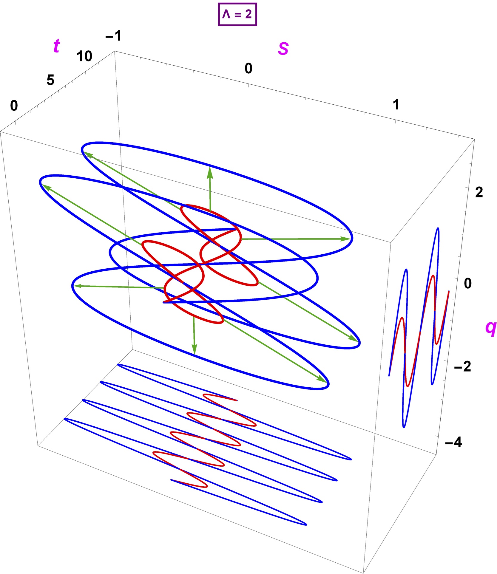
The space-alone rescaling lifts to Bargmann space as the homothety,
| (IV.7) |
and generates there a chrono-projective symmetry for null geodesics 5Chrono ; DGH91 ; KHarmonies ; Conf4GW , as shown on Fig.1. The associated conserved quantity is (II.13).
Let us consider two motions and which start from the same initial position but with different initial velocities, The space-alone rescaling takes into . Both motions return to their initial position after a half period (since the latter is independent of the initial conditions, as purportedly observed by Galilei in the Pisa cathedral).
V Gravitational waves and oscillators
Let us now consider the exact gravitational plane wave studied by Brinkmann Brinkmann ,
| (V.1a) | |||
| (V.1b) | |||
where and are the and polarization-state amplitudes. A simple example is given by the -independent linearly polarized gravitational wave Brdicka with and , i.e.,
| (V.2) |
Viewed as a Bargmann space, this metric describes an attractive oscillator in the coordinate combined with a repulsive (inverted) one in the sector ; corresponds to non-relativistic time (as anticipated). The motion is governed by the geodesic Lagrangian
| (V.3) |
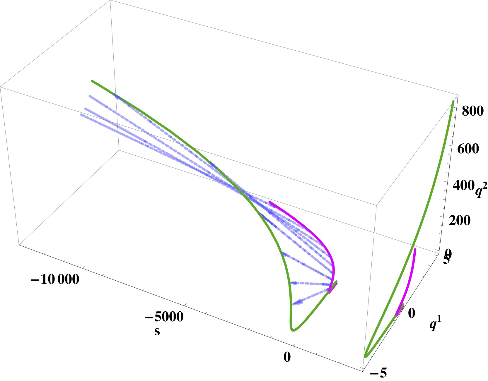
where the dot denotes derivation w.r.t. an affine parameter. For a particle initially at rest (e.g. with initial conditions ) the trajectory is,
| (V.4) |
shown on fig.2. Then the homothety (IV.7) Torre ; AndrPrenc ; Conf4GW generated by
| (V.5) |
is a chrono-projective transformation 5Chrono of the metric (V.2),
| (V.6) |
The associated conserved charge is
| (V.7a) | |||
| (V.7b) | |||
Evaluating the integral, .
We remark that changing the relative sign from minus to plus in (V.2),
| (V.8) |
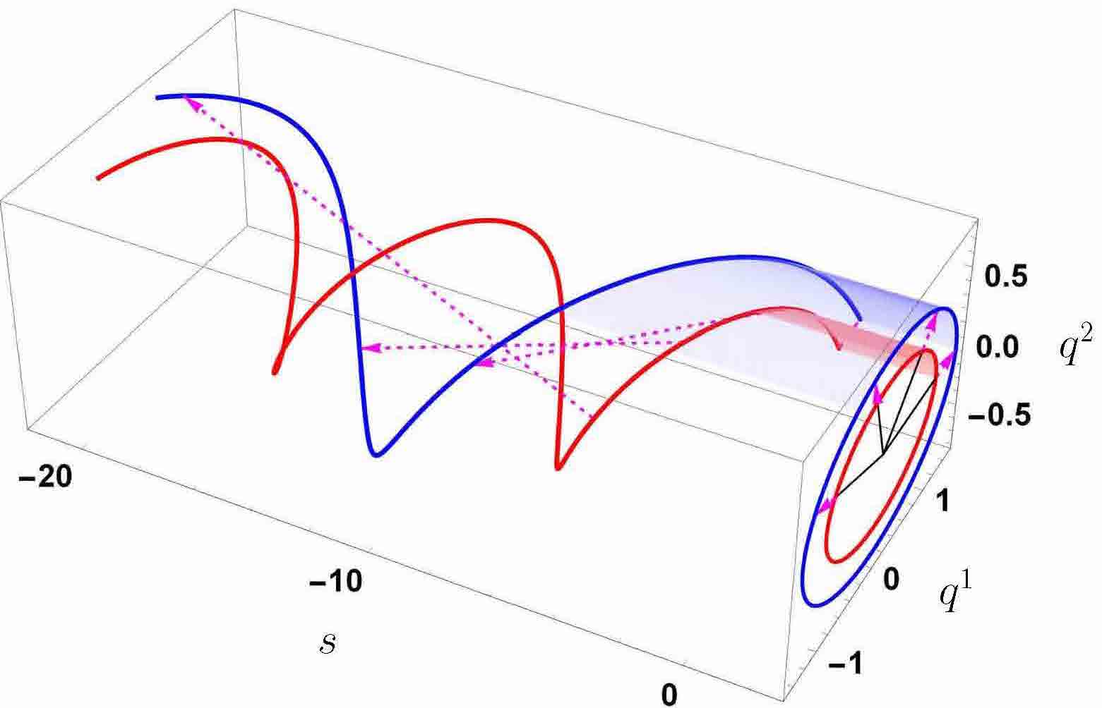
would yield instead the Bargmann description of a time independent isotropic harmonic oscillator 555 (V.8) is only a pp wave, not a vacuum solution of the Einstein equations Brinkmann ; DGH91 .. The familiar elliptic trajectories in the transverse plane lift to Bargmann space as null geodesics ; the -preserving isometries span the centrally extended Newton-Hooke group, whose -preserving conformal extension spans a group isomorphic to the Schrödinger group, etc. Here we just mention that the homothety (V.5) acts as a chrono-projective symmetry. The associated Noether charge is still , yielding the projected conserved quantity (V.7a)
| (V.9) |
with the isotropic oscillator Lagrangian . Fig.3 should be compared with the Kepler figure in KHarmonies .
VI Discussion
In this paper we extended Noether’s theorem to more general symmetry transformations which include also rescalings. Our results confirm the conserved charge found recently KHarmonies for the Kepler problem; for a free particle we recover Schrödinger dilations JacobiLec ; Schr . For homogeneous potential (which include free fall and a harmonic oscillator) we get a new charge, whose conservation allows us we rederive the virial theorem. Further applications (namely to gravitational plane waves) will be presented elsewhere Conf4GW .
Compared with the usual Noether theorem, our new charge (II.4) has has an extra term, in fact the classical action, which can be calculated only after the equations of motion had been solved. The new conservation law has nevertheless useful applications, as demonstrated by its use to prove the virial theorem and to derive Kepler’s Third law KHarmonies .
Further applications and generalizations are discussed in Conf4GW where it is argued that a similar conserved quantity arises for exact plane waves, and behaves as a symmetry for null geodesics motion Carroll4GW ; POLPER ; Ilderton . The extension to massive geodesics is considered in Dimakis .
We just mention that Maxwell’s electromagnetic Lagrangian under duality transformations would provide a field-theoretical example with helicity as associated conserved quantity.
After our paper was first posted to arXiv, our attention was called to earlier investigations vKampen ; Nachtergaele . The closest to our approach is that van Kampen vKampen , who uses also a Lagrangian framework ; his equation # (5) is in fact our eqn. (II.1). He could have [but did not] obtain our new charge (II.4) by integrating his unnumbered equation after his # (5) on p.237.
Nachtergaele et al. Nachtergaele studied canonical transformations in the Hamiltonian framework in symplectic space, and applied them to Toda chains.
Both of these papers focus on the virial theorem related to the Kepler rescaling ; no additional conserved quantity was found, though.
We also came across Keplar which uses Lie transformations and would also allow to derive our new charge (II.4). Our approach here is based instead on chrono-projective transformations DThese ; 5Chrono in the context of E-D lifts to Bargmann manifolds, which are gravitational wave spacetimes Eisenhart ; Bargmann ; DGH91 . Also ref. Igata discusses similar issues.
Acknowledgements.
We are indebted to Gary Gibbons for advice and Bruno Nachtergaele for correspondance. ME thanks the Denis Poisson Institute of Orléans - Tours University for a post-doctoral scholarship. This work was partially supported by National Natural Science Foundation of China (Grant No. 11575254). P.K. was supported by the grant 2016/23/B/ST2/00727 of the National Science Centre of Poland.References
- (1) L. Landau and E. Lifchitz, Physique Théorique, Tome I: Mécanique. édition. Éditions MIR, Moscou (1969); V. Arnold, Les méthodes mathématiques de la mécanique classique, Éditions MIR, Moscou (1976).
- (2) P.-M. Zhang, M. Cariglia, M. Elbistan, G. W. Gibbons and P. A. Horvathy, “”Kepler Harmonies” and conformal symmetries,” Physics Letters B 792 (2019) 324 [arXiv:1903.01436 [gr-qc]]. https://doi.org/10.1016/j.physletb.2019.03.057
- (3) L. P. Eisenhart, “Dynamical trajectories and geodesics”, Annals Math. 30 591-606 (1928).
- (4) C. Duval, G. Burdet, H. P. Künzle and M. Perrin, “Bargmann structures and Newton-Cartan theory”, Phys. Rev. D 31 (1985) 1841.
- (5) C. Duval, G.W. Gibbons, P. Horvathy, “Celestial mechanics, conformal structures and gravitational waves,” Phys. Rev. D43 (1991) 3907. [hep-th/0512188].
- (6) P.-M. Zhang, M. Cariglia, M. Elbistan and P. A. Horvathy, “Scaling and conformal symmetries for plane gravitational waves,” [arXiv:1905.08661 [gr-qc]].
- (7) C. Duval, “Quelques procédures géométriques en dynamique des particules,” Doctorat d’Etat ès Sciences (Aix-Marseille-II), 1982 (unpublished). See also G. Burdet, C. Duval and M. Perrin, “Cartan Structures On Galilean Manifolds: The chrono-projective Geometry,” J. Math. Phys. 24 (1983) 1752. doi:10.1063/1.525927.
- (8) M. Perrin, G. Burdet and C. Duval, “chrono-projective Invariance of the Five-dimensional Schrödinger Formalism,” Class. Quant. Grav. 3 (1986) 461. doi:10.1088/0264-9381/3/3/020
- (9) M. Cariglia, “Null lifts and projective dynamics,” Annals Phys. 362 (2015) 642 doi:10.1016/j.aop.2015.09.002 [arXiv:1506.00714 [math-ph]].
- (10) C. G. J. Jacobi, “Vorlesungen über Dynamik.” Univ. Königsberg 1842-43. Herausg. A. Clebsch. Vierte Vorlesung: Das Princip der Erhaltung der lebendigen Kraft. Zweite ausg. C. G. J. Jacobi’s Gesammelte Werke. Supplementband. Herausg. E. Lottner. Berlin Reimer (1884).
- (11) R. Jackiw, “Introducing scaling symmetry,” Phys. Today, 25 (1972) 23; U. Niederer, “The maximal kinematical symmetry group of the free Schrödinger equation,” Helv. Phys. Acta 45 (1972) 802 C. R. Hagen, “Scale and conformal transformations in Galilean-covariant field theory,” Phys. Rev. D5 (1972) 377.
- (12) V. de Alfaro, S. Fubini and G. Furlan, “Conformal Invariance in Quantum Mechanics,” Nuovo Cim. A 34 (1976) 569. doi:10.1007/BF02785666
- (13) M. Henkel, “Local Scale Invariance and Strongly Anisotropic Equilibrium Critical Systems,” Phys Rev. Lett. 78 (1997), 1940 ; “Phenomenology of local scale invariance: from conformal invariance to dynamical scaling,” Nucl. Phys. B 641 (2002) 405
- (14) C. Duval and P. A. Horvathy, “Non-relativistic conformal symmetries and Newton-Cartan structures,” J. Phys. A 42 (2009) 465206 doi:10.1088/1751-8113/42/46/465206 [arXiv:0904.0531 [math-ph]]
- (15) G. S. Hall and J. D. Steele, “Conformal vector fields in general relativity,” J. Math. Phys. 32 (1991) 1847. doi:10.1063/1.529249 ; G. S. Hall, “Symmetries and Curvature Structure in General Relativity”, World Scientific (2004).
- (16) M. W. Brinkmann, “Einstein spaces which are mapped conformally on each other,” Math. Ann. 94 (1925) 119–145.
- (17) M. Brdička, “On Gravitational Waves,” Proc. Roy. Irish Acad. 54A (1951) 137.
- (18) C. G. Torre, “Gravitational waves: Just plane symmetry,” Gen. Rel. Grav. 38 (2006) 653 doi:10.1007/s10714-006-0255-8 [gr-qc/9907089].
- (19) K. Andrzejewski and S. Prencel, “Memory effect, conformal symmetry and gravitational plane waves,” Phys. Lett. B 782 (2018) 421 doi:10.1016/j.physletb.2018.05.072 [arXiv:1804.10979 [gr-qc]].
- (20) C. Duval, G. W. Gibbons, P. A. Horvathy and P.-M. Zhang, “Carroll symmetry of plane gravitational waves,” Class. Quant. Grav. 34 (2017). doi.org/10.1088/1361-6382/aa7f62. [arXiv:1702.08284 [gr-qc]].
- (21) P. M. Zhang, C. Duval, G. W. Gibbons and P. A. Horvathy, “Velocity Memory Effect for Polarized Gravitational Waves,” JCAP 1805 (2018) no.05, 030 doi:10.1088/1475-7516/2018/05/030 [arXiv:1802.09061 [gr-qc]].
- (22) A. Ilderton, “Screw-symmetric gravitational waves: a double copy of the vortex,” Phys. Lett. B 782 (2018) 22 doi:10.1016/j.physletb.2018.04.069 [arXiv:1804.07290 [gr-qc]].
- (23) N. Dimakis, P. A. Terzis and T. Christodoulakis, “Integrability of geodesic motions in curved manifolds through non-local conserved charges,” Phys. Rev. D 99 (2019) no.10, 104061 doi:10.1103/PhysRevD.99.104061 [arXiv:1901.07187 [gr-qc]].
- (24) N.G. Van Kampen, “Transformation Groups and the Virial Theorem,” Reports on Math. Physics 3, 235 (1972).
- (25) B. Nachtergaele and A. Verbeure, “Groups of canonical transformations and the virial-Noether theorem,” Journal of Geometry and Physics, 3, 315-325 (1986)
- (26) N. Ogawa, “A Note on the scale symmetry and Noether current,” hep-th/9807086.
- (27) T. Igata, “Scale invariance and constants of motion,” PTEP 2018 (2018) no.6, 063E01 doi:10.1093/ptep/pty060 [arXiv:1804.03369 [hep-th]].