Elastic energy regularization for inverse obstacle scattering problems

Abstract

By introducing a shape manifold as a solution set to solve inverse obstacle scattering problems we allow the reconstruction of general, not necessarily star-shaped curves. The bending energy is used as a stabilizing term in Tikhonov regularization to gain independence of the parametrization. Moreover, we discuss how self-intersections can be avoided by penalization with the Möbius energy and prove the regularizing property of our approach as well as convergence rates under variational source conditions.

In the second part of the paper the discrete setting is introduced, and we describe a numerical method for finding the minimizer of the Tikhonov functional on a shape-manifold. Numerical examples demonstrate the feasibility of reconstructing non-star-shaped obstacles.

Keywords: Shape spaces, inverse obstacle scattering, nonlinear Tikhonov regularization

1 Introduction

Inverse obstacle scattering problems consist of reconstructing the shape of an impenetrable or homogeneous scattering obstacle from measurements of scattered waves. Such problems, which occur for example in structural health monitoring and medical imaging, have been studied intensively, see the monographs [12, 14, 26, 39] and references therein.

One may distinguish two main classes of reconstruction methods for inverse obstacle scattering problems: Sampling methods and parameterization-based methods. In sampling methods, an indicator function $f\colon\mathbb{R}^{d}\to\mathbb{R}\cup\{\infty\}$ is constructed based on the measured data, such that the value of $f$ indicates whether a point belongs to the obstacle or not (at least for noise-free data). Examples include the linear sampling method [1, 12, 13], the factorization method [25, 26], and the singular source method [38, 39].

In contrast, parameterization-based methods yield a parameterization of some approximation of the true obstacle. Examples include decomposition methods [15, 27] and iterative regularization methods [23], in particular, regularized Newton methods [20, 36] and nonlinear Tikhonov regularization.

Both sampling and parameterization-based methods have their respective advantages and disadvantages. On the one hand, sampling methods do not require a-priori knowledge of the obstacle’s topology and often not even of the boundary condition. They are typically easy to implement. On the other hand, they often require (i) a lot of data (e.g., the complex-valued far-field patterns for all incident fields); are (ii) less flexible concerning modifications of the forward problem (e.g., amplitude measurements or nonlinearities); and yield (iii) less accurate reconstructions than parameterization-based methods. Ideally, both types of methods can complement each other by using a sampling method to construct an initial guess for a parameterization-based method (see Remark 3 below).

For parameterization-based methods, one seeks approximate parameterizations of the unknown curve within a chosen class of boundary curves. In existing literature, this class is often chosen in a rather ad hoc manner. E.g., the obstacle is assumed to be star-shaped with respect to some known point such that the boundary can be described by a positive, periodic radial function. In this manner, one can formulate inverse obstacle problems as operator equations in Hilbert spaces. In this case, the attendant penalty terms are usually represented in the form of Sobolev norms of the parameterization. However, such norms crucially depend on the choice of the parameterization and thus disobey the geometry of the shape to be reconstructed. Indeed, a single curve $\mathbb{S}^{1}\to\mathbb{R}^{2}$ admits a continuum of possible parameterizations and therefore, parameterization-dependent norms break symmetry in an unnatural manner. Moreover, the assumption of star-shaped obstacles is severely restrictive.

Our contribution is the introduction of the boundary curve’s bending energy as a regularizing term for the two-dimensional case. This approach is purely geometric and independent of the choice of any parameterization and thus allows for arbitrary planar curves (of sufficient regularity). Considering the set of curves as geometric objects, independent of any particular parameterization, is of course a well established paradigm by now in the context of shape spaces. Michor and Mumford [33] showed that the space of closed regular curves (of sufficient regularity) carries the structure of a Riemannian manifold. This ansatz leads to certain degeneracies of geodesics and has therefore subsequently been refined and extended is several directions, e.g., using curvature-weighted $L^{2}$-metrics [34], $L^{2}$-metrics that incorporate a curve’s stretching and bending contributions [45, 46], and certain Sobolev-type metrics [5, 6, 10, 11]. In particular, curvature-based (i.e., second order) formulations penalize a curve’s bending contributions and lead to physically plausible simulations of thin elastic rods and threads [4, 7, 41]. In the discrete setting, curvature-based energies can be approximated using polygonal (piecewise straight) curves. Convergence in Hausdorff distance of the resulting minimizers (under suitable boundary conditions and a length constraint) to their smooth counterparts was recently shown in [44], which provides one of the theoretical underpinnings of the current work. We discuss the attendant discrete model in Section 5.

We argue that the use of shape manifolds may be largely preferable over parameterization-dependent methods, and the use of bending energy may be beneficial whenever regularization is applied to the set of curves in form of a penalization. In this paper we focus on Tikhonov regularization since it has the simplest and most complete convergence analysis. Our main theoretical result is the regularizing property of Tikhonov regularization on shape manifolds and convergence rates under variational source conditions.

The plan of the rest of this paper is as follows: We introduce our shape-manifold of curves as well as the requisite bending energy functional on this manifold in the next section. Our main theoretical results on the regularizing property and convergence rates of the proposed method are contained in Section 3. We then introduce the sound-soft obstacle scattering problem as a typical example of a forward problem and derive some properties of the forward operator defined on the shape manifold in Section 4. In Section 5 we describe our discrete model of the shape manifold and explain how to solve the associated minimization problem. We finally present our numerical results in Section 6 and combine it with a sampling method in section 7.

2 Shape manifold and elastic energy

In this section we introduce the shape manifold of closed curves $\varGamma$ in ${\mathbb{R}}^{2}$ and investigate its structure. We further define an energy functional on this manifold.

The shape manifold

Let $\varGamma\subset{\mathbb{R}}^{2}$ be a regular, closed curve of class $H^{2}$ of length $L$, i.e., there is a parameterization $\gamma\in H^{2}([0,1],{\mathbb{R}}^{2})$ satisfying $\gamma^{\prime}(t)\neq 0$ for all $t\in[0,1]$ and the closing conditions

$$\gamma(0)=\gamma(1)\quad\text{and}\quad\gamma^{\prime}(0)=\gamma^{\prime}(1).$$ (1)

Without loss of generality, we may assume that $\gamma$ is of constant speed, i.e., $\lvert{\gamma^{\prime}(t)}\rvert=L$. Thus, we may represent $\gamma$ by a triple $m=(\theta,L,p)$ with a base point $p\coloneqq\gamma(0)$, the curve’s length $L$, and an angle function $\theta\in H^{1}([0,1],{\mathbb{R}})$ via

$$\gamma(t)=\gamma_{m}(t)\coloneqq p+\int_{0}^{t}\gamma^{\prime}(\tau)\,{\mathrm{d}}\tau=p+L\int_{0}^{t}\,\big{(}\cos(\theta(\tau)),\sin(\theta(\tau))\big{)}\,{\mathrm{d}}\tau.$$ (2)

In order to fulfill the closing conditions (1), $\theta$ needs to satisfy

$$\int_{0}^{1}\cos(\theta(t))\,{\mathrm{d}}t=0,\quad\int_{0}^{1}\sin(\theta(t))\,{\mathrm{d}}t=0\quad\text{and}\quad\theta(1)-\theta(0)\in 2\,\pi\,{\mathbb{Z}}.$$ (3)

The number $\frac{\theta(1)-\theta(0)}{2\,\pi}$ is called the turning number of $\gamma$ (not to be confused with the winding number). A necessary (but not sufficient) condition for $\varGamma$ to be embedded is that $\gamma$ has turning number $\pm 1$. Since our application focuses on boundary curves of simply connected domains, we may restrict ourselves to curves of turning number $+1$ and define the space:

$$\varTheta\coloneqq\big{\{}\theta\in H^{1}([0,1],{\mathbb{R}})\,\big{|}\,\textstyle\int_{0}^{1}\big{(}\cos(\theta(t)),\sin(\theta(t))\big{)}\,{\mathrm{d}}t=0,\;\theta(1)-\theta(0)=2\,\pi\big{\}}.$$

Lemma 1.

The space $\varTheta$ is an embedded submanifold of $H^{1}([0,1],{\mathbb{R}})$.

Proof.

We may write $\varTheta=\set{\theta\in E}{\varPhi(u)=0}$ with the affine subspace $E=\set{\theta\in H^{1}([0,1],{\mathbb{R}})}{\theta(1)-\theta(0)=2\,\pi}$ and the smooth mapping $\varPhi\colon E\to{\mathbb{R}}^{2}$,

$$\varPhi(\theta)=\int_{0}^{1}\big{(}\!\cos(\theta(t)),\sin(\theta(t))\big{)}\,{\mathrm{d}}t.$$

By virtue of the implicit function theorem, all that we have to do is to show that $\varPhi$ is a submersion, i.e. that $D\varPhi(\theta)$ admits a bounded linear right inverse for each $\theta\in E$ (see [31, Chapter II, §2]). Notice that $E$ is an affine subspace over the linear subspace

$$H^{1}_{\mathrm{per}}([0,1],{\mathbb{R}})\coloneqq\big{\{}u\in H^{1}([0,1],{\mathbb{R}})\,\big{|}\,u(0)=u(1)\big{\}}$$

and that

$$D\varPhi\,u=\begin{pmatrix}-\int_{0}^{1}\sin(\theta(t))\,u(t)\,{\mathrm{d}}t\\ \hphantom{-}\int_{0}^{1}\cos(\theta(t))\,u(t)\,{\mathrm{d}}t\end{pmatrix}.$$

Thus, it suffices to construct a $u\in H^{1}_{\mathrm{per}}([0,1],{\mathbb{R}})$ solving $D\varPhi\,u=\lambda$ and depending linearly on the right hand side for any prescribed $\lambda\in{\mathbb{R}}^{2}$. We set $s(t)\coloneqq\sin(\theta(t))$ and $c(t)\coloneqq\cos(\theta(t))$ and make the ansatz $u(t)=a\,s(t)+b\,c(t)$, which leads to the linear equation

$$\begin{pmatrix}-\langle s,s\rangle&-\langle s,c\rangle\\ \langle c,s\rangle&\langle c,c\rangle\end{pmatrix}\begin{pmatrix}a\\ b\end{pmatrix}=\begin{pmatrix}\lambda_{1}\\ \lambda_{2}\end{pmatrix},$$

where $\langle\cdot,\cdot\rangle$ denotes the $L^{2}$ inner product. By Cauchy-Schwarz, the determinant of this system is negative since $\theta(t)$ is continuous and not constant. ∎

The tangent space of $\varTheta$ is given by

$$T_{\theta}\varTheta=\big{\{}u\in H^{1}_{\mathrm{per}}([0,1],{\mathbb{R}})\,\big{|}\,\textstyle D\varPhi(\theta)\,u=0\big{\}}.$$

The family of inner products $(g_{\theta})_{\theta\in\varTheta}$ defined by

$$g_{\theta}(u,v)\coloneqq\int_{0}^{1}\big{(}u(t)\,v(t)+u^{\prime}(t)\,v^{\prime}(t)\big{)}\,{\mathrm{d}}t\quad\text{for $u$, $v\in T_{\theta}\varTheta$}$$

turns $(\varTheta,g)$ into a infinite-dimensional Riemannian manifold (in the sense of [31]).

For a compact, convex set of base points $B\subset{\mathbb{R}}^{2}$ and for bounds of acceptable curve lengths, we define our space of feasible curves by

$$\mathcal{M}\coloneqq\varTheta\times[L_{1},L_{2}]\times B.$$

Then $\mathcal{M}$ is a smooth submanifold with corners in the Hilbert space

$$\mathbb{X}\coloneqq H^{1}([0,1],{\mathbb{R}})\times{\mathbb{R}}\times{\mathbb{R}}^{2}$$

and its tangent space at an interior point $m=(\theta,L,p)$ is given by

$$T_{m}\mathcal{M}=T_{\theta}\varTheta\oplus{\mathbb{R}}\oplus{\mathbb{R}}^{2}.$$

Elastic energy

Continuing our geometric approach, recall that the Euler-Bernoulli bending energy (see [16]) of a planar curve $\varGamma$ is given by

$$\int_{\varGamma}\kappa^{2}\,{\mathrm{d}}s,$$

where ${\mathrm{d}}s$ is the line element and $\kappa$ denotes the (signed) curvature of $\varGamma$. The bending energy, or more precisely the curvature, is a geometrical invariant of the curve $\varGamma$ and thus we gain independence under reparameterizations, which is the main benefit of our approach. The bending energy models the stored deformation energy of $\varGamma$ under the assumption of an undeformed straight rest state of the same length as $\varGamma$.

Let $\varGamma$ be parameterized by $\gamma$ that is represented by $m=(\theta,L,p)\in\mathcal{M}$ as in (2). Then we have $\kappa(t)=\frac{\theta^{\prime}(t)}{L}$ and ${\mathrm{d}}s=L\,{\mathrm{d}}t$. This shows that bending energy scales with $1/\lambda$ when $\varGamma$ is re-scaled by a factor $\lambda>0$. Thus, without any additional constraints, minimizers of this energy do not exist (the energy of $\gamma_{m}$ converges to $0$ for $L\to\infty$). We therefore consider the following scale-invariant version $\mathcal{E}_{\mathrm{b}}\colon\mathcal{M}\to[0,\infty)$ of bending energy which is simply the $H^{1}$-seminorm:

$$\mathcal{E}_{\mathrm{b}}(m)\coloneqq\int_{0}^{1}{\theta^{\prime}(t)}^{2}\,{\mathrm{d}}t.$$ (4)

As mentioned above, $\mathcal{E}_{\mathrm{b}}(m)$ describes the energy required to deform a straight elastic rod of length $L$ into $\varGamma$. More generally, consider an undeformed rest state $\varGamma_{*}$ of non-vanishing curvature (i.e., if $\varGamma_{*}$ is pre-curved). Assuming that $\varGamma_{*}$ is deformed into $\varGamma$ by a diffeomorphism $\varphi\colon\varGamma_{*}\to\varGamma$ that does not change the line element, bending energy is given by

$$\int_{\varGamma_{*}}(\kappa_{*}(s)-\kappa(\varphi(s)))^{2}\,{\mathrm{d}}s.$$

Representing $\varGamma_{*}$ by $m_{*}=(\theta_{*},L,p_{*})$ as above, the scale-invariant version of this energy is given by

$$\mathcal{E}_{\mathrm{b}}(m,m_{*})=\int_{0}^{1}(\theta^{\prime}(t)-\theta_{*}^{\prime}(t))^{2}\,{\mathrm{d}}t.$$

This formulation is useful when $\varGamma_{*}$ represents a reasonable initial guess that is further optimized in order to obtain the desired solution.

Non-self-intersecting curves

When reconstructing a domain, one requires a boundary curve that is free of self-intersections. In this context, the following lemma is useful.

Lemma 2.

The set of non-self-intersecting curves is open in the $\mathbb{X}$-topology.

Proof.

First notice that curves of finite bending energy correspond to elements of the Sobolev space $H^{2}([0,1],{\mathbb{R}}^{2})$. Furthermore, by construction, each member of $\mathcal{M}$ represents a $C^{1}$-immersion $\gamma\colon\mathbb{S}^{1}\to\mathbb{R}^{2}$; indeed, due to periodic boundary conditions we can take $\mathbb{S}^{1}$ as the domain for $\gamma$. Since injective immersions of compact domains are embeddings, we may employ Theorem 3.10 from [35], stating that the set of $C^{1}$-embeddings is open in $C^{1}(\mathbb{S}^{1},\mathbb{R}^{2})$. Now, the fact that $H^{2}(\mathbb{S}^{1},\mathbb{R}^{2})$ embeds continuously into $C^{1}(\mathbb{S}^{1},\mathbb{R}^{2})$ implies the result. ∎

Remark 3.

If a sufficiently good initial guess $m_{*}\in\mathcal{M}$ of the true solution is available and if $m_{*}$ is free of self-intersections, then Lemma 2 ensures that we can choose

$$\mathcal{M}_{0}\coloneqq\set{m\in\mathcal{M}}{\|m-m_{*}\|_{\mathbb{X}}\leq\delta}$$ (5)

containing only non-self-intersecting curves. In the context of inverse obstacle scattering problems such an initial guess can often be constructed by sampling methods as discussed in the introduction and in Section 7.

Although we have not encountered the problem of self-intersections in practice for our method, we briefly outline how to avoid this issue whenever needed. A popular and widely studied energy that is self-avoiding (i.e., finite energy guarantees that the curve is free of self-intersections) is the so-called Möbius energy defined as

$$\mathcal{E}_{\mathrm{M}}(\varGamma)\coloneqq\int_{\varGamma}\int_{\varGamma}\bigg{(}\frac{1}{|x-y|^{2}}-\frac{1}{d_{\varGamma}(x,y)^{2}}\bigg{)}\,{\mathrm{d}}s(x)\,{\mathrm{d}}s(y),$$ (6)

where $d_{\varGamma}(x,y)$ denotes the geodesic distance between $x$ and $y$ along $\varGamma$ and integration is performed with respect to the line elements. This parameterization-invariant energy was introduced by O’Hara [37] and its analytical properties have been studied by several authors [8, 9, 18, 21, 29, 30]. The self-avoiding property is ensured by the first summand of the integrand, while the second summand is introduced in order to remove the singularity along the diagonal $x=y$. The Möbius energy is invariant under Möbius transformations (i.e., under conformal transformations of ${\mathbb{C}}\cong{\mathbb{R}}^{2}$) and thus in particular scale-invariant. We will show in Section 3 that using the Möbius energy as an additional penalty term ensures that minimizers of the regularized problem are indeed free of self-intersections.

Properties of the energy functionals

The analysis of well-posedness and convergence properties of Tikhonov regularization in Section 3 requires some properties of the energy functionals $\mathcal{E}_{\mathrm{b}}$ and $\mathcal{E}_{\mathrm{M}}$ on the Riemannian manifold $\mathcal{M}$. For showing existence of solutions via the direct method of the calculus of variations, weakly sequential lower semi-continuity of the objective functional is a desirable property. Weak convergence, however, is a concept that is not invariant under nonlinear changes of coordinates. Because we parameterized $\mathcal{M}$ as in (2), the bending energy becomes a convex quadratic functional, enabling us to derive the following result.

Proposition 4.

Let ${\mathcal{E}}\in\set{\mathcal{E}_{\mathrm{b}},\mathcal{E}_{\mathrm{b}}(\cdot,m_{*})}$. With respect to the $\mathbb{X}$-topology, we have:

1. $\mathcal{M}\subset\mathbb{X}$ is weakly sequentially closed.

2. ${\mathcal{E}}$ is weakly sequentially lower semi-continuous.

3. Modulo shifts by elements of $2\,\pi\,{\mathbb{Z}}$ , the sublevel sets ${\mathcal{E}}^{-1}([0,a])\subset\mathcal{M}$ are weakly sequentially compact.

Proof.

We proceed in the usual manner of the direct method of calculus of variations. In order to show (i), consider a sequence $(m_{n}=(\theta_{n},L_{n},p_{n}))_{n\in\mathbb{N}}$ in $\mathcal{M}$ that converges weakly to some $m=(\theta,L,p)\in\mathcal{M}$. By the Rellich compactness theorem, $H^{1}([0,1],{\mathbb{R}})$ is compactly embedded in $C([0,1],{\mathbb{R}})$ equipped with the supremum norm. Thus, weak convergence of $\theta_{n}\rightharpoonup\theta$ in $H^{1}([0,1],{\mathbb{R}})$ implies strong convergence in $C([0,1],{\mathbb{R}})$. Since the closing conditions (3) are continuous on $C([0,1],{\mathbb{R}})$, this implies that $\theta\in\varTheta$ and thus $m\in\mathcal{M}$.
In order to show (ii), notice that ${\mathcal{E}}$ is defined in terms of a squared seminorm on $\mathbb{X}$, which is a continuous and convex functional, whose sublevel sets are therefore sequentially closed and convex. The fact that sequentially closed convex sets are weakly sequentially closed implies (ii).
For showing (iii), we first observe that for each $z\in 2\,\pi\,{\mathbb{Z}}$, the curve represented by $(\theta+z,L,p)$ is the same as the one represented by $(\theta,L,p)$. Now let $m_{n}=(\theta_{n},L_{n},p_{n})$ be a sequence in a sublevel set ${\mathcal{E}}^{-1}([0,a])$. Modulo shifting by $z_{n}\in 2\,\pi\,{\mathbb{Z}}$, we may assume that $\theta_{n}(0)\in\left[0,2\pi\right]$. We may define an equivalent norm on $H^{1}([0,1],{\mathbb{R}})$ by $\|\theta\|_{*}\coloneqq\lvert{\theta(0)}\rvert+\lVert{\theta^{\prime}}\rVert_{L^{2}}$. We then either have $\lVert{\theta_{n}}\rVert_{H^{1}}\leq 2\,\pi+\sqrt{{\mathcal{E}}(\theta_{n})}$ (for the case of ${\mathcal{E}}=\mathcal{E}_{\mathrm{b}}$) or $\lVert{\theta_{n}-\theta_{*}}\rVert_{H^{1}}\leq 2\,\pi+|\theta_{*}(0)|+\sqrt{{\mathcal{E}}(\theta_{n})}$ (for the case of ${\mathcal{E}}=\mathcal{E}_{\mathrm{b}}(\cdot,m_{*})$). In either case, the sequence $(m_{n})_{n\in\mathbb{N}}$ is bounded in $H^{1}$, and hence it has a subsequence $(\theta_{n_{k}})$ converging weakly to some $\theta\in H^{1}([0,1],{\mathbb{R}})$. Moreover, $\left[L_{1},L_{2}\right]\times B$ is compact so that we may find a further subsequence so that $m_{n_{k}}$ converges weakly to some $m=(\theta,L,p)\in H^{1}([0,1],{\mathbb{R}})\times\left[L_{1},L_{2}\right]\times B$. Because of (ii), we have ${\mathcal{E}}(m)\leq a$ and because of (i), $m$ is indeed an element of $\mathcal{M}$. ∎

Lemma 5.

The Möbius energy $\mathcal{E}_{\mathrm{M}}\colon\mathcal{M}\to[0,\infty]$ defined by (6) is weakly sequentially lower semi-continuous with respect to the weak topology of $\mathbb{X}$.

Proof.

Recall that (2) constitutes a smooth mapping from $\mathcal{M}$ to $H^{2}(S^{1},{\mathbb{R}}^{2})$. As shown in [9], the Möbius energy is continuously differentiable (and thus continuous) on the space of embeddings of class $C^{0,1}(S^{1},{\mathbb{R}}^{2})\cap H^{3/2}(S^{1},{\mathbb{R}}^{2})$. Now the statement follows from the compactness of the embedding of $H^{2}(S^{1},{\mathbb{R}}^{2})$ into this space. More precisely, let $m_{n}$, $m\in\mathcal{M}$ with $m_{n}\rightharpoonup m$. We have to show that $\mathcal{E}_{\mathrm{M}}(m)\leq c\coloneqq\liminf_{n\to\infty}\mathcal{E}_{\mathrm{M}}(m_{n})$. In the case of $c=\infty$, there is nothing to show, so assume that $c<\infty$. Since $\mathcal{E}_{\mathrm{M}}$ is invariant under scaling and translation, we may assume that $L_{n}=L=1$ and $p_{n}=p=0$. Denote by $\gamma_{n}$, $\gamma\in H^{2}(S^{1},{\mathbb{R}}^{2})$ the corresponding parameterizations. Due to the Rellich embedding, we may pick a subsequence such that $c=\lim_{k\to\infty}\mathcal{E}_{\mathrm{M}}(m_{n_{k}})$ and such that $\gamma_{n_{k}}\to\gamma$ strongly in $C^{0,1}\cap H^{3/2}$. The latter shows that

$$\mathcal{E}_{\mathrm{M}}(m)=\lim_{k\to\infty}\mathcal{E}_{\mathrm{M}}(m_{n_{k}})=c,$$

which proves the claim. ∎

3 Tikhonov regularization

In this section we consider a general injective operator

$$F\colon\mathcal{M}_{0}\subset\mathcal{M}\to\mathbb{Y}$$

mapping a set of embedded curves $\mathcal{M}_{0}$ into a Hilbert space $\mathbb{Y}$. The unknown exact solution will be denoted by $m^{\dagger}\in\mathcal{M}_{0}$. Noisy data is described by a vector $y^{\delta}\in\mathbb{Y}$ satisfying

$$\|y^{\dagger}-F(m^{\dagger})\|_{\mathbb{Y}}\leq\delta.$$

In order to approximately recover $m^{\dagger}$ from the data $y^{\delta}$, we use Tikhonov regularization with some regularization parameter $\alpha>0$:

$$m_{\alpha}^{\delta}\in\operatorname{argmin}_{m\in\mathcal{M}_{0}}\left[\|F(m)-y^{\delta}\|_{\mathbb{Y}}^{2}+\alpha\,\mathcal{E}_{\mathrm{b}}(m,m_{*})\right].$$ (7)

Here $m_{*}$ denotes an initial guess of $m^{\dagger}$ and may be set to $0$ if no such initial guess is available. If no appropriate submanifold of embedded curves $\mathcal{M}_{0}$ containing the true solution is known, we may choose $\mathcal{M}_{0}$ by setting $\mathcal{M}_{0}\coloneqq\set{m\in\mathcal{M}}{\mathcal{E}_{\mathrm{M}}(m)\leq c}$ for sufficiently large $c>0$ or alternatively consider Tikhonov regularization of the form

$$m_{\alpha}^{\delta}\in\operatorname{argmin}_{m\in\mathcal{M}}\left[\|F(m)-y^{\delta}\|_{\mathbb{Y}}^{2}+\alpha\,\mathcal{E}_{\mathrm{b}}(m,m_{*})+\alpha\,\mathcal{E}_{\mathrm{M}}(m)\right].$$ (8)

Since $\mathcal{E}_{\mathrm{M}}(m)=\infty$ if $m$ is self-intersecting, $\mathcal{E}_{\mathrm{M}}$ acts as a barrier function: Only the values of $F$ on the set of embedded curves are relevant and each curve $\gamma_{m_{\alpha}^{\delta}}$ is guaranteed to be embedded.

With the properties of the energy functionals established in the previous section, the following convergence properties follow from the general theory of nonlinear Tikhonov regularization.

Theorem 6.

Assume that $\mathcal{M}_{0}\subset\mathcal{M}$ contains only non-self-intersecting elements and let $m^{\dagger}\in\mathcal{M}_{0}$. Suppose that $F\colon\mathcal{M}_{0}\to\mathbb{Y}$ is weakly sequentially continuous (with respect to the topologies of $\mathbb{X}$ and $\mathbb{Y}$) and injective and $\mathcal{M}_{0}$ is weakly closed in the case of (7).

1. (existence) The infimum of the Tikhonov functionals in (7) and (8) is attained for any $\alpha>0$.

2. (regularizing property) Suppose that $F$ is injective. Moreover, consider a sequence of data $(y^{\delta_{n}})$ with $\|y^{\delta_{n}}-F(m^{\dagger})\|\leq\delta_{n}\to 0$ as $n\to\infty$. Assume that the regularization parameters are chosen such that

   $$\alpha_{n}\to 0\qquad\mbox{and}\qquad\frac{\delta_{n}}{\sqrt{\alpha_{n}}}\to 0\,.$$

   Then for any sequence of minimizers of the Tikhonov functionals we have

   $$\lim_{n\to\infty}\big{\lVert}{m_{\alpha_{n}}^{\delta_{n}}-m^{\dagger}}\big{\rVert}_{\mathbb{X}}=\lim_{n\to\infty}\big{\lVert}{\gamma_{m_{\alpha_{n}}^{\delta_{n}}}-\gamma_{m^{\dagger}}}\big{\rVert}_{\infty}=0,$$ (9)

   $$\lim_{n\to\infty}\big{\lVert}{F\big{(}m_{\alpha_{n}}^{\delta_{n}}\big{)}-F\big{(}m^{\dagger}\big{)}}\big{\rVert}_{\mathbb{Y}}=0.$$ (10)

3. (convergence rates) Suppose in the case of (7) that there exists a loss function $l\colon\mathcal{M}\times\mathcal{M}\to[0,\infty)$ and a concave, increasing function $\varphi\colon[0,\infty)\to[0,\infty)$ with $\varphi(0)=0$ such that $m^{\dagger}$ satisfies the variational source condition

   $$l(m,m^{\dagger})\leq\mathcal{E}_{\mathrm{b}}(m,m_{*})-\mathcal{E}_{\mathrm{b}}(m^{\dagger},m_{*})+\varphi\big{(}\|F(m)-F(m^{\dagger})\|_{\mathbb{Y}}^{2}\big{)}$$ (11)

   for all $m\in\mathcal{M}_{0}$. Then the reconstruction error for an optimal choice $\overline{\alpha}$ of $\alpha$ is bounded by

   $$l\big{(}m_{\overline{\alpha}}^{\delta},m^{\dagger}\big{)}\leq 2\,\varphi(\delta^{2}).$$ (12)

Proof.

We define a functional $\mathcal{E}\colon\mathbb{X}\to[0,\infty)$ by

$$\mathcal{E}(m)\coloneqq\begin{cases}\mathcal{E}_{\mathrm{b}}(m,m_{*}),&\mbox{if }m\in\mathcal{M}_{0},\\ \infty,&\mbox{else}\end{cases}\quad\mbox{or}\quad$$

$$\mathcal{E}(m)\coloneqq\begin{cases}\mathcal{E}_{\mathrm{b}}(m,m_{*})+\mathcal{E}_{\mathrm{M}}(m),&\mbox{if }m\in\mathcal{M},\\ \infty,&\mbox{else}\end{cases}$$

in the case of (7) or (8), respectively. We show that in both cases $\mathcal{E}$ is weakly sequentially lower semi-compact, i.e. sublevel-sets of $\mathcal{E}$ are weakly sequentially compact. In the first case this follows from Proposition 4, part (iii) and the assumption that $\mathcal{M}_{0}$ is weakly sequentially closed. In the second case this is a straightforward consequence of Proposition 4, part (iii) and Lemma 5.

Extending $F$ to an operator $\widetilde{F}\colon\mathbb{X}\to\mathbb{Y}$ in an arbitrary fashion, we can formally write the Tikhonov regularizations (7) and (8) as a minimization problem over $\mathbb{X}$,

$$m_{\alpha}^{\delta}\in\operatorname{argmin}_{m\in\mathbb{X}}\left[\|\widetilde{F}(m)-y^{\delta}\|_{\mathbb{Y}}^{2}+\alpha\,\mathcal{E}(m)\right].$$

and apply standard convergence results for generalized Tikhonov regularization. The first statement now follows from [42, Theorems 3.22] or [17, Theorems 3.2].

To prove the second statement, let $m^{\dagger}=(\theta^{\dagger},L^{\dagger},p^{\dagger})$ and $m_{\alpha_{n}}^{\delta_{n}}=(\theta_{n},L_{n},p_{n})$ and recall from [42, Theorem 3.26] or [17, Theorem 3.4] that (10) holds true, and for an injective operator we have weak convergence of $m_{\alpha_{n}}^{\delta_{n}}$ to $m^{\dagger}$ as well as $\lim_{n\to\infty}\mathcal{E}(m_{\alpha_{n}}^{\delta_{n}})=\mathcal{E}(m^{\dagger})$. Since $\mathcal{E}_{\mathrm{b}}$ and $\mathcal{E}_{\mathrm{M}}$ are both weakly sequentially lower semicontinuous it follows that $\lim_{n\to\infty}\|\theta_{n}^{\prime}-\theta_{*}^{\prime}\|_{L^{2}}^{2}=\|(\theta^{\dagger}-\theta_{*})^{\prime}\|_{L^{2}}^{2}$. This implies

$$\|(\theta_{n}-\theta^{\dagger})^{\prime}\|_{L^{2}}^{2} =\|(\theta_{n}-\theta_{*})^{\prime}\|_{L^{2}}^{2}-\|(\theta^{\dagger}-\theta_{*})^{\prime}\|_{L^{2}}^{2}+\langle{(\theta^{\dagger}-\theta_{*})^{\prime},(\theta_{n}-\theta^{\dagger})^{\prime}}\rangle_{L^{2}}$$

$$\to 0\qquad\mbox{as }n\to\infty.$$

Modulo shifts in $2\,\pi\,{\mathbb{Z}}$, we may assume that $\theta_{n}(0)\in\left[-\pi,\pi\right]$. By passing to a subsequence, we may assume that $\theta_{n_{k}}(0)\to\theta^{\dagger}(0)$. Using the equivalent norm $\|\theta\|_{*}\coloneqq\lvert{\theta(0)}\rvert+\lVert{\theta^{\prime}}\rVert_{L^{2}}$ on $H^{1}([0,1],\mathbb{R})$ this yields strong convergence of $(\theta_{n_{k}})$ to $\theta^{\dagger}$ in $H^{1}([0,1],\mathbb{R})$. As weak convergence in $\mathbb{R}^{2}$ is equivalent to strong convergence, $(L_{n_{k}},p_{n_{k}})$ also converges strongly to $(L^{\dagger},p^{\dagger})$. As this holds true for any subsequence, the whole sequence $(m_{\alpha_{n}}^{\delta_{n}})$ converges strongly to $m^{\dagger}$ in $\mathbb{X}$. This implies strong convergence of the corresponding curves in the supremum norm.

The third statement follows from [19] or [17, Theorem 4.11]. ∎

We point out that the variational source condition (11) is related to stability results as worked out for inverse medium scattering problems in [24] where such conditions with logarithmic functions $\varphi$ hold true under Sobolev smoothness conditions on the solution. However, for inverse obstacle scattering problems no such verifications of variational source conditions are known so far.

Remark 7.

It can be seen from the references cited in the proof of Theorem 6 that the results can be extended to the case where $\mathbb{Y}$ is a Banach space and $\|F(m)-y^{\delta}\|_{\mathbb{Y}}^{2}$ is replaced by more general data fidelity terms $\mathcal{S}(F(m),y^{\delta})$.

4 Inverse obstacle scattering problem

As a prominent example of an obstacle scattering problem we consider here the scattering of time-harmonic acoustic waves at a sound-soft cylindrical obstacle. The cross section of this obstacle is described by a bounded, connected, and simply connected Hölder $C^{1,\alpha}$-smooth domain $\varOmega_{\mathrm{int}}$ ($\alpha>0$). Then its unbounded complement $\varOmega\coloneqq\mathbb{R}^{2}\setminus\overline{\varOmega_{\mathrm{int}}}$ is connected, and the boundary curve will be denoted by $\varGamma=\partial\varOmega=\partial\varOmega_{\mathrm{int}}$. Further we consider an incident plane wave $u_{\mathrm{i}}(x)=\exp({\mathrm{i}}\,k\,\langle x,d\rangle)$ with wavenumber $k>0$ and direction $d\in\mathbb{S}^{1}$. Then the forward problem consists in finding a scattered wave $u_{\mathrm{s}}\in H^{2}_{\mathrm{loc}}(\varOmega)$ such that the total wave $u\coloneqq u_{\mathrm{i}}+u_{\mathrm{s}}$ solves the Helmholtz equation with Dirichlet boundary condition

$$\Delta u(x)+k^{2}u(x)=0,\qquad x\in\varOmega,$$ (13a)

$$u(x)=0,\qquad x\in\varGamma,$$ (13b)

together with the Sommerfield radiation condition

$$\lim_{\lvert x\rvert\to 0}\sqrt{\lvert x\rvert}\left(\frac{\partial u_{\mathrm{s}}(x)}{\partial\lvert x\rvert}-{\mathrm{i}}\,k\,u_{\mathrm{s}}(x)\right) =0$$ (13c)

which holds uniformly for all directions $\frac{x}{\lvert x\rvert}\in\mathbb{S}^{1}$. This problem is well-posed under the above conditions (see e.g. [32]) and can for example be solved using boundary integral equations (see [14]). Recall that solutions to the Helmholtz equation which satisfy the Sommerfield radiation condition (13c) have the asymptotic behavior

$$u_{\mathrm{s}}(x)=\frac{\mathrm{e}^{\mathrm{i}k\lvert x\rvert}}{\sqrt{\lvert x\rvert}}\left(u_{\infty}\left(\tfrac{x}{\lvert x\rvert},d\right)+\mathcal{O}\left(\tfrac{1}{\lvert x\rvert}\right)\right),\qquad\lvert x\rvert\to\infty$$ (14)

(see [14, Sect. 2.2 and 3.4]). The function $u_{\infty}(\cdot,d)$ is analytic on $\mathbb{S}^{1}$ and known as the far field pattern of the scattered wave $u_{\mathrm{s}}$. Often the far field pattern $u_{\infty}\in L^{2}(\mathbb{S}^{1}\times\mathbb{S}^{1})$ can only be measured on some submanifold $\mathbb{M}\subset\mathbb{S}^{1}\times\mathbb{S}^{1}$, e.g. $\mathbb{M}=\mathbb{S}^{1}\times\{d\}$ for one incident field or $\mathbb{M}=\{(d,-d)\colon d\in\mathbb{S}^{1}\}$ for backscattering data.

With the definitions of Section 2 we may describe the inverse problems as operator equations on the Riemannian manifold $\mathcal{M}$: We introduce the operator $F\colon\mathcal{M}\to L^{2}(\mathbb{M})$ mapping $m\in\mathcal{M}$ to the far field pattern $u_{\infty}$ of the scattered field in problem (13) for the domain $\varOmega$ corresponding to $m$. More precisely, the boundary $\varGamma$ is given by the image of the curve parameterization $\gamma_{m}(\mathbb{S}^{1})$ and $\varOmega$ is the unbounded component of $\mathbb{R}^{2}\setminus\gamma_{m}(\mathbb{S}^{1})$. The inverse problem is described by the operator equation

$$F(m)=u_{\infty}.$$ (15)

By Schiffer’s uniqueness result ([14, Theorem 5.1]) $F$ is injective if $\mathbb{M}=\mathbb{S}^{1}\times\mathbb{S}^{1}$, and by the uniqueness result of Colton and Sleeman ([14, Theorem 5.1]) it is also injective if $\mathbb{M}$ is the product of $\mathbb{S}^{1}$ with some finite set and if all curves $\gamma_{m}$ for $m\in\mathcal{M}_{0}$ are contained in a ball of a certain size. (Both results are stated in [14] for $\mathbb{R}^{3}$, but also hold true in $\mathbb{R}^{2}$.)

Let us show that the operator $F$ also satisfies the remaining assumptions of Theorem 6:

Proposition 8.

The operator $F$ maps weakly convergent sequences in $\mathcal{M}_{0}$ (with respect to the topology of $\mathbb{X}$) to strongly convergent sequences in $L^{2}(\mathbb{S}^{1})$ and is continuously Fréchet differentiable.
In particular, $F$ is strongly and weakly continuous.

Proof.

Notice that the linear mapping $\mathbb{X}\to C^{1}(\mathbb{S}^{1},\mathbb{R}^{2})$, $m\mapsto\gamma_{m}$ defined by (2) is compact by embedding theorems for Sobolev spaces, and hence it maps weakly convergent sequences to strongly convergent sequences. Moreover, the forward scattering operator $C^{1}(\mathbb{S}^{1},\mathbb{R}^{2})\to L^{2}(\mathbb{S}^{1})$, $\gamma_{m}\mapsto u_{\infty}$ is continuously Fréchet differentiable, and in particular continuous by [23, Theorem 1.9]. Therefore, the composition of these two mappings is continously Fréchet differentiable and maps weakly convergent to strongly convergent sequences. ∎

Notice that by the last proposition the operator equation (15) on an infinite dimensional manifold $\mathcal{M}_{0}$ is ill-posed in the sense that there cannot exist a strongly continuous inverse of $F$. (Otherwise every weakly convergent sequence in $\mathcal{M}_{0}$ would be strongly convergent.) This implies the need for regularization to solve this equation.

Remark 9 (translation invariance for phaseless data).

In many applications only the squared amplitude of the far field can be measured, but not the phase. As the amplitude of the far field is translation invariant (see [28]), the corresponding forward operator $F_{\mathrm{ampl}}(m)\coloneqq|F(m)|^{2}$ is also translation invariant, i.e. $F_{\mathrm{ampl}}(\theta,L,p)$ does not depend on the base point $p$. This case fits very well into our setting since the shape manifold may simply be reduced to $\mathcal{M}_{\mathrm{ampl}}\coloneqq\varTheta\times[L_{1},L_{2}]$.

5 Discrete setting

In order to treat bending energy computationally, we represent closed curves by closed polygons. To this end, consider an arbitrary (but fixed) partition $(0=\tau_{0}<\tau_{1}<\dots<\tau_{n}=1)$ of the unit interval and let the angle variable be given by a piecewise constant function represented by a vector $\bm{\theta}=(\theta_{1},\dots,\theta_{n})$, i.e. $\theta(t)=\theta_{j}$ for $t\in(\theta_{j-1},\theta_{j}]$. In perfect analogy to (2), we then define a polygon of length $L$ by

$$\gamma(t)\coloneqq p+L\int_{0}^{t}\,\big{(}\!\cos(\theta(\tau)),\sin(\theta(\tau))\big{)}\,{\mathrm{d}}\tau.$$ (16)

Analogously to the smooth case, in order to fulfill the closing conditions (1), $\bm{\theta}$ needs to satisfy

$$\varPhi(\bm{\theta})=0,\quad\mbox{where}\quad\varPhi(\bm{\theta})=\int_{0}^{1}\big{(}\!\cos(\theta(t)),\sin(\theta(t))\big{)}\,{\mathrm{d}}t.$$ (17)

Define the turning angles by $[\bm{\theta}]_{i}\coloneqq(\theta_{i+1}-\theta_{i})$, where indices are taken modulo $n$ and $[\bm{\theta}]_{i}$ is shifted such that $[\bm{\theta}]_{i}\in(-\pi,\pi]$ for all $i$. The number $\left(\sum_{i}[\bm{\theta}]_{i}\right)/2\pi$ is known as the discrete turning number of $\gamma$.

Let ${\varTheta}_{n}\coloneqq\{\bm{\theta}\in\mathbb{R}^{n}\,|\,\varPhi(\bm{\theta})=0\}$ and define the space of discrete curves by

$${\mathcal{M}}_{n}\coloneqq{\varTheta}_{n}\times[L_{1},L_{2}]\times B\quad\subset\quad{\mathbb{X}}_{n}\coloneqq{\mathbb{R}}^{n}\times{\mathbb{R}}\times{\mathbb{R}}^{2},$$

for a compact, convex set of base points $B\subset{\mathbb{R}}^{2}$ and minimal and maximal acceptable curve lengths $0<L_{1}\leq L_{2}<\infty$. On this space, the scale-invariant version of discrete bending energy for a curve $\bm{m}\in{\mathcal{M}}_{n}$ is readily defined as

$$\mathcal{E}_{\mathrm{b,n}}(\bm{m})\coloneqq\sum_{i=1}^{n}\left(\frac{[\bm{\theta}]_{i}}{h_{i}}\right)^{2}h_{i}\,=\,\sum_{i=1}^{n}\frac{([\bm{\theta}]_{i})^{2}}{h_{i}},$$ (18)

see, e.g., [22]. Here the dual edge lengths are given by $h_{i}\coloneqq(\tau_{i+1}-\tau_{i-1})/2$ for $i\in\{1,\dots,n\}$, where we set $\tau_{n+1}=1+\tau_{1}$. This expression provides the natural analogue of the smooth version (4). It goes back to the work of Hencky in his 1921 PhD thesis [22] and is in the spirit of discontinuous Galerkin (DG) methods ([3]). A completely analogous discrete version of this energy can be defined for open polygons. In this case, for clamped boundary conditions and under the constraint of fixed total curve length, the set of minimizers of this discrete energy converges in Hausdorff distance to the corresponding set of smooth minimizers under mesh refinement, see [44]. More specifically, the angle variables converge in $L^{\infty}$ and in $W^{1,p}$ for $p\in[2,\infty)$ under a suitable smoothing operator for the angle variables. Finally, a discrete analogue $\mathcal{E}_{\mathrm{b,n}}(\bm{m},\bm{m}_{*})$ of the smooth pre-curved energy $\mathcal{E}_{\mathrm{b}}(m,m_{*})$ is readily obtained by replacing $[\bm{\theta}]$ by $([\bm{\theta}]-[\bm{\theta}]_{*})$ in (18).

Implementation details

For convenience, we briefly sketch here the implementation of our method. The regularized functional that we seek to minimize on the space ${\mathcal{M}}_{n}\subset{\mathbb{X}}_{n}$ is of the form

$${\mathcal{J}}^{\alpha}\colon{\mathcal{M}}_{n}\to{\mathbb{R}},\quad\bm{m}\mapsto\tfrac{1}{2}\big{\lVert}{{F}_{n}(\bm{m})-\bm{y}^{\delta}}\big{\rVert}_{{\mathbb{Y}}_{n}}^{2}+\alpha\,{\mathcal{E}}_{n}(\bm{m}).$$ (19)

Here, ${F}_{n}:{\mathcal{M}}_{n}\to{\mathbb{Y}}_{n}$ is some discretization for polygonal closed curves of the forward operator $F$, the term $\bm{y}^{\delta}\in{\mathbb{Y}}_{n}$ represents the measured data in some finite dimensional Euclidean space ${\mathbb{Y}}_{n}$, the scalar $\alpha\geq 0$ is the regularization parameter, and ${\mathcal{E}}_{n}=\mathcal{E}_{\mathrm{b,n}}$ or ${\mathcal{E}}_{n}=\mathcal{E}_{\mathrm{b,n}}+\mathcal{E}_{\mathrm{M,n}}$ with a discrete approximation $\mathcal{E}_{\mathrm{M,n}}$ of the Möbius energy $\mathcal{E}_{\mathrm{M}}$.

Remark 10.

We skip the requisite details on the definition of $\mathcal{E}_{\mathrm{M,n}}$ since our numerical experiments show that in practice the tracking term $\tfrac{1}{2}\big{\lVert}{{F}_{n}(\bm{m})-\bm{y}^{\delta}}\big{\rVert}_{{\mathbb{Y}}_{n}}^{2}$ (see (19) below) is sufficient to prevent iterates from developing self-intersections. Notwithstanding, for details on discrete Möbius energy, see [29, 30], and for $\varGamma$-convergence to the smooth case see [43].

The discrete nonlinear Tikhonov regularization on ${\mathcal{M}}_{n}$ may then be written as the following constrained minimization problem:

$$\text{Minimize}\;\;{\mathcal{J}}^{\alpha}(\bm{m})\;\;\text{subject to}\;\;\varPhi(\bm{m})=0\;\;\text{and}\;\;(L,p)\in[L_{1},L_{2}]\times B.$$ (20)

We will ignore the inequality constraints $(L,p)\in[L_{1},L_{2}]\times B$ for simplicity, although it would not be difficult to include them. In particular, these constraints never became active in our numerical experiments. We only require these constraints for the theoretical analysis in Section 3.

Since ${F}_{n}$ does not have a natural extension outside the discrete shape space ${\mathcal{M}}_{n}=\{\bm{m}\,|\,\varPhi(\bm{m})=0\}$, standard methods of constrained nonlinear programming are not applicable. When using iterative methods for minimizing ${\mathcal{J}}^{\alpha}$, we require an intrinsic stepping method on the constraint manifold ${\mathcal{M}}_{n}$ in order to supply the forward operator ${F}_{n}$ with meaningful input. Prominent examples of such methods are intrinsic Newton-type algorithms on Riemannian manifolds, see, e.g., [40]. In such methods, one determines the update direction $\bm{u}\in{\mathbb{X}}_{n}$ by solving a saddle point system of the form

$$\begin{pmatrix}H(\bm{m})&D\varPhi^{\top}(\bm{m})\\ D\varPhi(\bm{m})&0\end{pmatrix}\begin{pmatrix}\bm{u}\\ \mu\end{pmatrix}=\begin{pmatrix}-D{\mathcal{J}}^{\alpha}(\bm{m})\\ 0\end{pmatrix},$$ (21)

where $H$ is (a surrogate for) the Hessian of the objective functional, the manifold ${\mathcal{M}}_{n}$ is given by the constraint equations (17), which we encode by a function $\varPhi:{\mathbb{X}}_{n}\to{\mathbb{R}}^{2}$, and $\mu\in\mathbb{R}^{2}$ denotes a Lagrange multiplier. The resulting linear systems have roughly the size $n\times n$ and can be solved using a direct solver. In our implementation, we usually use $n=100$.

A first example is the full intrinsic Hessian, which can be obtained from the Lagrange function $\mathcal{L}(\bm{m},\lambda)\coloneqq{\mathcal{J}}^{\alpha}(\bm{m})+\lambda^{\top}\varPhi(\bm{m})$ of (20) as

$$H(\bm{m})=D_{\bm{m}}^{2}\mathcal{L}(\bm{m},\lambda_{\bm{m}})=D^{2}{\mathcal{J}}^{\alpha}(\bm{m})+\lambda_{\bm{m}}^{\top}D^{2}\varPhi(\bm{m}).$$ (22)

The requisite Lagrange multiplier $\lambda_{\bm{m}}^{\top}\in\mathbb{R}^{2}$ is obtained by multiplying the equation $D_{\bm{m}}\mathcal{L}(\bm{m},\lambda)=0$ by $D\varPhi^{\dagger}(\bm{m})$ from the right, i.e.,

$$\lambda_{\bm{m}}^{\top}=-D{\mathcal{J}}^{\alpha}(\bm{m})\,D\varPhi^{\dagger}(\bm{m}).$$

Here $D\varPhi^{\dagger}(\bm{m})$ denotes the Moore-Penrose inverse with respect to a finite difference approximation of the $H^{1}$-inner product.

Notice that assembling the system with the full intrinsic Hessian contains a contribution of the form $\langle{{F}_{n}(\bm{m})-\bm{y}^{\delta},D^{2}{F}_{n}(\bm{m})(\cdot,\cdot)}\rangle_{{\mathbb{Y}}_{n}}$, which is dense and costly to compute. We therefore use a Gauß-Newton inspired surrogate, which is given in bilinear form as

$$H(\bm{m})=\langle{D{F}_{n}(\bm{m})\,\cdot\,,D{F}_{n}(\bm{m})\,\cdot\,}\rangle_{{\mathbb{Y}}_{n}}+\alpha\operatorname{Hess}{\mathcal{E}}_{n}(\bm{m}),$$ (23)

where we identify matrices with bilinear forms and where the intrinsic energy Hessian has the form

$$\operatorname{Hess}{\mathcal{E}}_{n}(\bm{m})=D^{2}{\mathcal{E}}_{n}(\bm{m})-D{\mathcal{E}}_{n}(\bm{m})\,D\varPhi^{\dagger}(\bm{m})D^{2}\varPhi(\bm{m}).$$ (24)

Notice that the second term on the right hand side of this equation arises from the second term on the right hand side of (22). In the language of differential geometry, the term $D\varPhi^{\dagger}(\bm{m})\,D^{2}\varPhi(\bm{m})$ encodes the second fundamental form of the constraint manifold. The quantities on the right hand side of (24) are easy to assemble for ${\mathcal{E}}_{n}=\mathcal{E}_{\mathrm{b,n}}$ due to the quadratic nature of $\mathcal{E}_{\mathrm{b,n}}$.

Another attractive alternative is to use

$$H(\bm{m})=\langle{D{F}_{n}(\bm{m})\,\cdot\,,D{F}_{n}(\bm{m})\,\cdot\,}\rangle_{{\mathbb{Y}}_{n}}+\alpha\,\langle{\cdot,\cdot}\rangle_{\mathbb{X}}.$$

This way, $H(\bm{m})$ is always positive definite on the null space of $D\varPhi(\bm{m})$ and the saddle-point matrix from (21) is guaranteed to be continuously invertible. Thus, in this case, the method boils down to a gradient descent in the manifold ${\mathcal{M}}_{n}$ with respect to the Riemannian metric induced by $H$.

Once an update direction $\bm{u}$ has been computed in the above fashion, the next iterate is found by first setting $\bm{x}_{0}=\bm{m}+t\,\bm{u}$ for some small $t>0$. Restoring feasibility (i.e., ensuring that the next iterate resides on the constraint manifold) is then achieved by iterating

$$\bm{x}_{k+1}=\bm{x}_{k}-D\varPhi^{\dagger}(\bm{x}_{k})\,\varPhi(\bm{x}_{k}),$$ (25)

until $\varPhi(\bm{x}_{k})$ is sufficiently small. The step size $t$ can be determined by a standard backtracking line search, while the matrix-vector product $\tilde{\bm{u}}=D\varPhi^{\dagger}(\bm{x})\,\tilde{\bm{v}}$ is computed by solving the saddle point problem

$$\begin{pmatrix}G_{{\mathbb{X}}_{n}}&D\varPhi^{\top}(\bm{x})\\ D\varPhi(\bm{x})&0\end{pmatrix}\begin{pmatrix}\tilde{\bm{u}}\\ \tilde{\mu}\end{pmatrix}=\begin{pmatrix}0\\ \tilde{\bm{v}}\end{pmatrix}.$$

Here $G_{{\mathbb{X}}_{n}}$ is the Gram matrix of the discrete $H^{1}$-inner product on ${\mathbb{X}}_{n}$, the upper left $n\times n$ block of which is a finite-difference Laplacian. Analoguously, $D\mathcal{E}_{\mathrm{b,n}}(\bm{m})\,D\varPhi^{\dagger}(\bm{m})=(D\varPhi^{\dagger}(\bm{m}))^{\top}D\mathcal{E}_{\mathrm{b,n}}(\bm{m})$ can be computed this way by utilizing the dual saddle point system. Finally, one updates $\bm{m}$ to the last iterate $\bm{x}_{k}$.

6 Ab-initio reconstructions

In this section we demonstrate the benefits of our new approach in numerical experiments for the inverse obstacle scattering problem introduced in Section 4. The forward scattering problems were solved by a boundary integral equation method using a Nyström method with $n$ points as described in [14, sec. 3.6]. To this end we interpolated the polygonal curve approximations described in section 5 trigonometrically. Both the evaluation of discrete forward operator ${F}_{n}$ and the evaluation of its Jacobian $D{F}_{n}$ as described e.g. in [23] require $\mathcal{O}(n^{3})$ flops.

We always use 20 equidistant incident plane waves and $n=100$ points for the reconstruction curves; the far field pattern is measured at 40 equidistant measurement directions. The wavelength is chosen of the same order of magnitude as the diameter of the obstacle. In all our examples we added independent, identically distributed, centered Gaussian random variables to the simulated far field data at each sampling point such that the relative noise level in the $l^{2}$-norm was $5\%$ (in Figures 1, 2 and 3) or $1\%$ (in Figures 4 and 5).

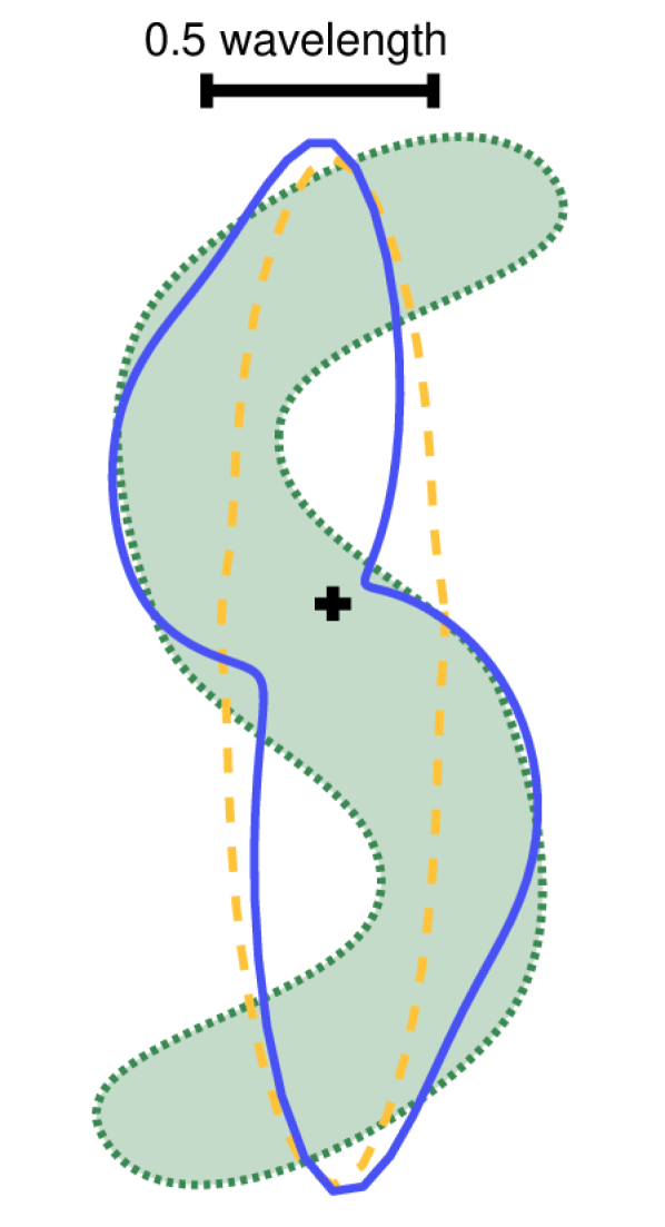
(a)

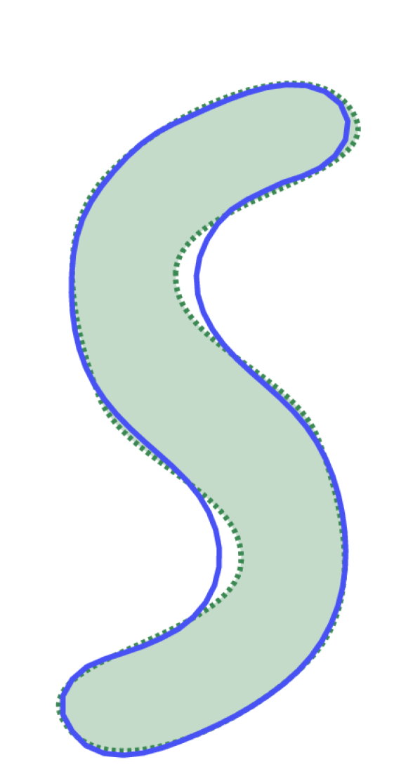
(b)

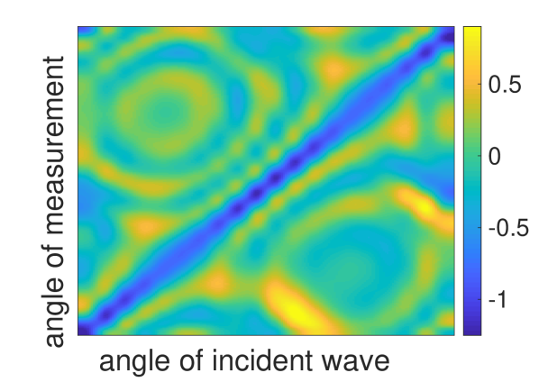
(c)

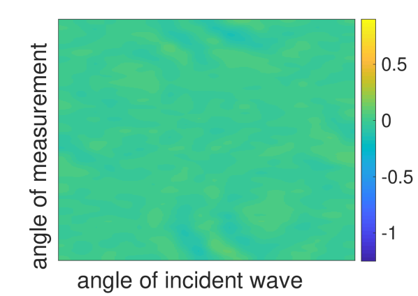
(d)

Figure 1: Comparison of our method (b) to previous radial function parameterizations (a) for a smooth non-star-shaped domain. We use 20 equidistant incident waves with wavelength indicated in (a) and $5\%$ Gaussian white noise. (a) true obstacle (dotted green), initial guess (dashed yellow), and reconstruction (solid blue) using a radial function parameterization with center indicated by the black cross; (b) reconstruction using bending energy penalization; (c) real part of far field of the reconstruction in (b); (d) difference to the observations of the real parts of reconstructed far field in (b).

The regularization parameter $\alpha$ was determined by the discrepancy principle. More precisely, we first minimized the Tikhonov functional for a large $\alpha$ by an intrinsic Gauss-Newton-type method as described in Section 5 with update direction $\bm{u}$ defined by (21), (23), (24). The Gauss-Newton iteration was stopped when $\|\bm{u}\|$ or the norm of the gradient of the Tikhonov functional $\|D{\mathcal{J}}^{\alpha}(\bm{m})\|$ was smaller than $10^{-5}$. Then we decreased $\alpha$ by a factor of $2$ and minimized the Tikhonov functional for this smaller $\alpha$ using the previous minimizer as an initial guess as long as the condition $\left\lVert{F}_{n}(\bm{m}_{\alpha})-\bm{y}^{\delta}\right\rVert\geq 1.1\delta$ was satisfied.

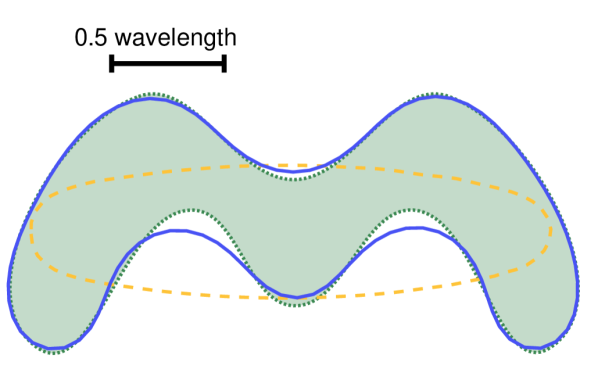
(a)

(b)

Figure 2: Reconstruction of a smooth non-star-shaped domain by our method with $5\%$ Gaussian white noise. Parameters, line styles and colors are chosen as in Figure 1. Panel (b) shows a magnification of reconstructions for different numbers of points ($n=50$, $100$, and $150$) illustrating the asymptotic independence of the results on the choice of $n$.

In Figures 1 and 2 we show reconstructions of two non-star-shaped domains. Figure 1 (d) illustrates that the far field pattern is uniformly fitted well. Moreover, we demonstrate in Figure 2 (b) that the reconstructions are almost independent of the choice of the number $n$ of points on the curves as long as $n$ is large enough. Also the number of Gauß-Newton steps and the regularization parameter $\alpha$ determined by the discrepancy principle do not depend on $n$. Note that concave parts of the boundary where multiple reflections occur in a geometrical optics approximation are more difficult to reconstruct than convex parts. In view of the fact that we use only one wave length which is almost of the size of the obstacle and a noise level of $5\%$, these reconstructions for this exponentially ill-posed problem are already remarkably good. The reconstructions could be further improved by using shorter wave lengths as illustrated in Figure 5 (c).

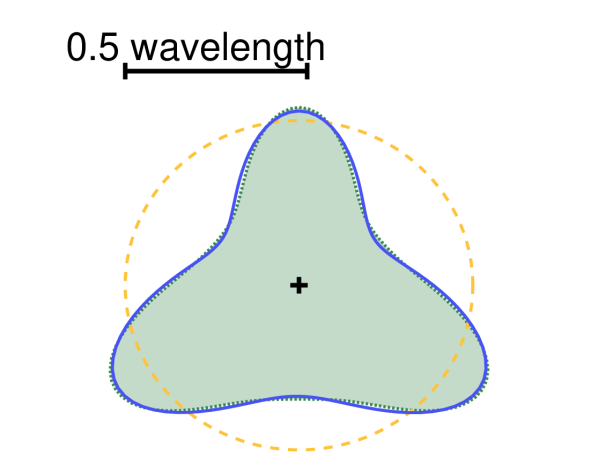
(a)

(b)

(c)

(d)

(e)

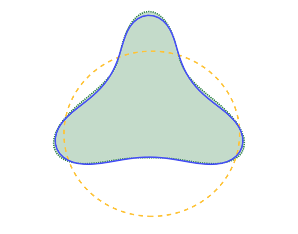
(f)

Figure 3: Comparison of our method to previous radial function parameterizations for a star-shaped domain. Parameters and line styles are chosen as in Figure 1. (a),(b),(d) show reconstructions using a radial function parameterization with different choices of the center point indicated by a black cross; (c), (e) are magnifications of (b) and (d) around the center point, respectively; (f) shows the reconstruction by our bending energy approach.

Figure 3 (a) already illustrates the obvious limitation of the commonly used radial function parameterizations to star-shaped domains. In Figure 3 we demonstrate a further disadvantage of such parameterizations, which is the dependence on the choice of the center point. We can observe unwanted deformations in the reconstruction or even a failure if the center point is chosen too close to the boundary of the exact domain. This is expected since the penalty term corresponding to the exact solution explodes as the origin tends to the boundary. In contrast, in the proposed approach based on the bending energy the position of the obstacle with respect to the origin has no influence on the global minimum of the Tikhonov functional (although local minimization methods will get stuck in local minima if the initial guess is too far away from the true obstacle).

We summarize that the proposed approach for solving inverse obstacle problems on a shape manifold with bending energy penalization may yield considerably better reconstructions than radial function parameterizations even for star-shaped obstacles and allows the reconstruction of considerably more complicated curves.

7 Reconstructions with initial guesses provided by sampling methods

The factorization method

Let us briefly recall the factorization method as an example of a sampling method and typical numerical implementations of this method. Suppose that $\mathbb{M}=\mathbb{S}^{1}\times\mathbb{S}^{1}$ and denote the integral operator with kernel $u_{\infty}$ by $U_{\infty}\in L(L^{2}(\mathbb{S}^{1}))$, i.e.

$$(U_{\infty}g)(\widehat{x})\coloneqq\int_{\mathbb{S}^{1}}u_{\infty}(\widehat{x},d)\,g(d)\,\mathrm{d}s(d),\qquad\widehat{x}\in\mathbb{S}^{1}.$$

Moreover, let $r_{z}(\widehat{x})\coloneqq\exp(-{\mathrm{i}}\,k\,\widehat{x}^{\top}z)$ denote the far field pattern of a point source at $z\in\mathbb{R}^{2}$. The main result justifying the factorization method (see [25, Theorem 3.8]) is that

$$r_{z}\in\mathrm{ran}(U_{\infty}^{*}U_{\infty})^{1/4}\quad\Leftrightarrow\quad z\in\varOmega_{\mathrm{int}}.$$

In practice, given only a discrete and noisy version of $U_{\infty}$, one constructs an approximation $A$ to the operator $(U_{\infty}^{*}U_{\infty})^{-1/4}$ (e.g. by a trunctated eigenvalue decomposition) and uses sublevel sets of the function

$$\chi(z)\coloneqq\|A\,r_{z}\|^{2}$$ (26)

as approximations of $\varOmega_{\mathrm{int}}$ since for continuous noiseless data $\chi(z)<\infty$ (with an appropriate definition of $\chi$) if and only if $z\in\varOmega_{\mathrm{int}}$. There are several variants concerning the choice of $A$ which follow the same pattern (see [2]).

In order to find a parameterization of some level line of a function $\chi\in C^{1}(\mathbb{R}^{2})$ in the form (2) we introduce the forward operator $F_{1/\chi}\colon\mathcal{M}\to L^{2}([0,2\pi])$ defined by

$$\left(F_{1/\chi}(m)\right)(t)\coloneqq\frac{1}{\chi(\gamma_{m}(t))},\qquad t\in[0,2\pi].$$

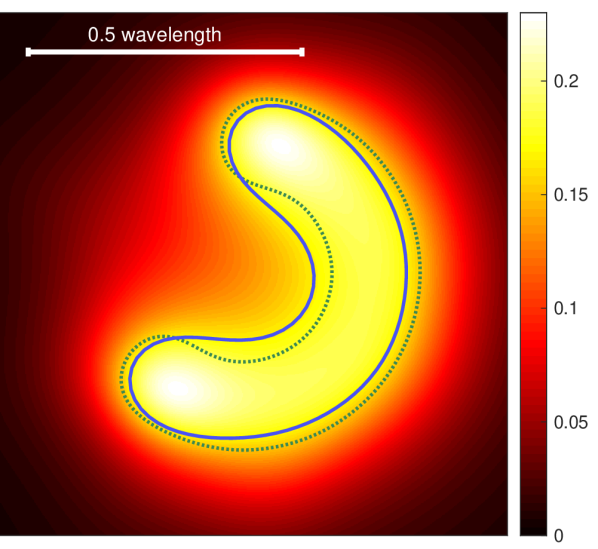
Figure 4: Obstacle reconstruction by parameterization of a level line for the factorization method. We use 20 incident waves and $1\%$ Gaussian white noise. The values of the function $1/\chi$ with $\chi$ given by (26) are indicated by colors and the true obstacle by a dotted green line. The solid blue line shows a parameterized level line of $1/\chi$ approximating the true obstacle.

Then the problem to find a parameterization of the $\beta$-level-line of $\chi$ can be formulated as an operator equation $F_{1/\chi}(m)=\beta\,\mathbf{1}$ where $\mathbf{1}\in L^{2}([0,2\pi])$ is the constant $1$ function. This problem may again be solved by Tikhonov regularization. The use of $F_{1/\chi}$ yields a more global convergence behavior than the use of $F_{\chi}$. Notice that $F_{1/\chi}$ is Fréchet differentiable with $(DF_{1/\chi}(m)\,h)(t)=-\chi(m(t))^{-2}\,\langle\operatorname{grad}\chi(\gamma_{m}(t)),\gamma_{h}(t)\rangle$. Notice that for $\chi$ given by (26), we have $\partial_{z_{j}}\chi(z)=2\Re\langle A\,r_{z},A\,\partial_{z_{j}}r_{z}\rangle$.

The reconstruction of a level line of $\chi$ (or equivalently $1/\chi$) is illustrated in Figure 4 using data corrupted by $1\%$ Gaussian white noise.

Numerical results

We now use the parameterization of the level line curve illustrated in Figure 4 as an initial guess $m_{*}$ in Tikhonov regularization. The result is shown in Figure 5 (b). In most parts the reconstruction is hard to distinguish from the true curve by eye, and it is much better than a reconstruction using a circle as initial guess as shown in Figure 5 (a). Only in some interior parts of the “horseshoe” the reconstruction in (b) seems to take a “short cut”. A reason may be that the initial guess curve $\gamma_{m_{*}}$ is “too short” in the interior part, and consequently geodesic distances of points on $\gamma_{m_{*}}$ relative to its length $L_{*}$ do not match the geodesic distances of their best approximations on $\gamma_{m^{\dagger}}$ relative to $L^{\dagger}$. Therefore, the bending energy $\mathcal{E}_{\mathrm{b}}(m^{\dagger},m_{*})$ is quite large whereas due to the “short cut” in the Tikhonov estimator $m_{\alpha}$ the bending energy $\mathcal{E}_{\mathrm{b}}(m_{\alpha},m_{*})$ is much smaller. However, as illustrated in Figure 5 (c), for smaller wavelengths the difference of the corresponding data fidelity terms becomes large enough to compensate for this effect.

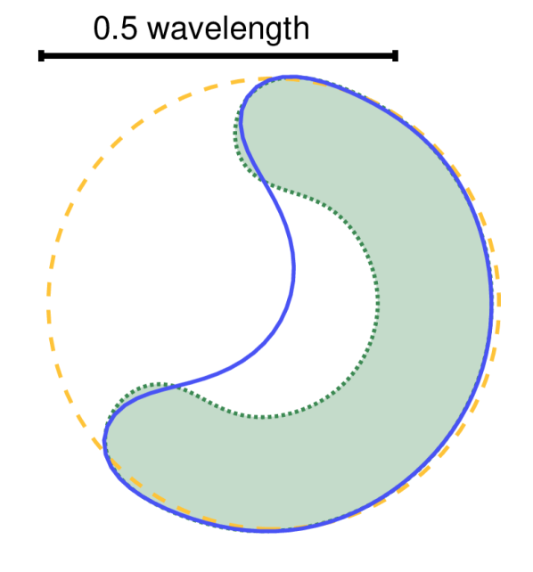
(a)

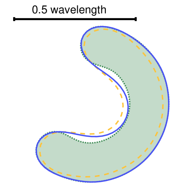
(b)

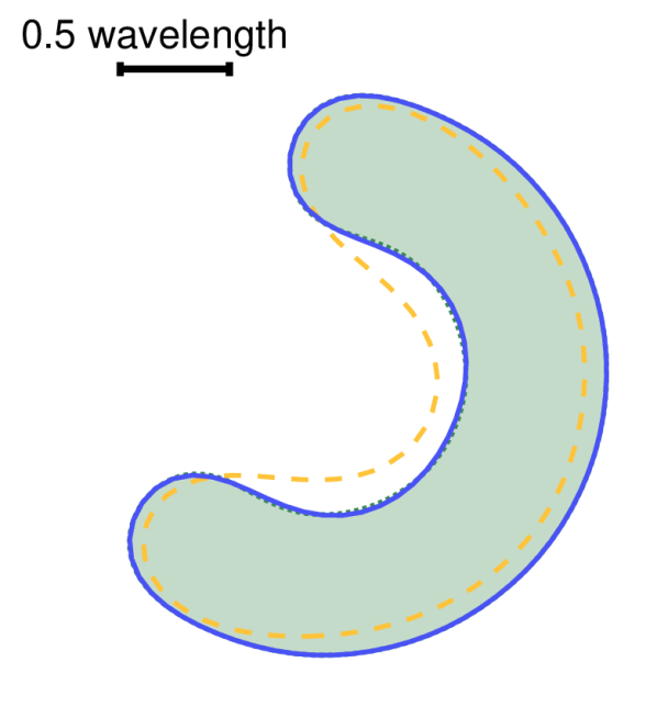
(c)

Figure 5: Reconstructions by our method for different initial guesses and different wave numbers. We use far field data with $1\%$ Gaussian white noise and otherwise the same parameters and line styles as in Figure 1. In panel (a) the initial guess (dashed yellow) is chosen as a circle, in panels (b) and (c) the initial guess is taken from the factorization method as illustrated in Figure 4. The reconstruction in (c) uses far field data for a smaller wavelength.

References

- [1] T. Arens and A. Lechleiter. The linear sampling method revisited. The Journal of Integral Equations and Applications, pages 179–202, 2009.
- [2] T. Arens and A. Lechleiter. Indicator functions for shape reconstruction related to the linear sampling method. SIAM Journal on Imaging Sciences, 8(1):513–535, 2015.
- [3] D. N. Arnold, F. Brezzi, B. Cockburn, and L. D. Marini. Unified analysis of discontinuous Galerkin methods for elliptic problems. SIAM J. Numer. Anal., 39(5):1749–1779, 2001/02.
- [4] B. Audoly, N. Clauvelin, P.-T. Brun, M. Bergou, E. Grinspun, and M. Wardetzky. A discrete geometric approach for simulating the dynamics of thin viscous threads. Journal of Computational Physics, 253:18–49, 2013.
- [5] M. Bauer, M. Bruveris, S. Marsland, and P. W. Michor. Constructing reparametrization invariant metrics on spaces of plane curves. Differential Geom. Appl., 34:139–165, 2014.
- [6] M. Bauer, M. Bruveris, and P. W. Michor. Why use Sobolev metrics on the space of curves. In P. Turaga and A. Srivastava, editors, Riemannian computing in computer vision, pages 223–255. Springer, 2016.
- [7] M. Bergou, M. Wardetzky, S. Robinson, B. Audoly, and E. Grinspun. Discrete Elastic Rods. ACM Transactions on Graphics (Proceedings of SIGGRAPH), 27(3):63:1–63:12, 2008.
- [8] S. Blatt. Boundedness and regularizing effects of O’Hara’s knot energies. J. Knot Theory Ramifications, 21(1):1250010, 9, 2012.
- [9] S. Blatt, P. Reiter, and A. Schikorra. Harmonic analysis meets critical knots. Critical points of the Möbius energy are smooth. Trans. Amer. Math. Soc., 368(9):6391–6438, 2016.
- [10] M. Bruveris. Completeness properties of Sobolev metrics on the space of curves. J. Geom. Mech., 7(2):125–150, 2015.
- [11] M. Bruveris, P. W. Michor, and D. Mumford. Geodesic completeness for Sobolev metrics on the space of immersed plane curves. Forum Math. Sigma, 2, 2014.
- [12] F. Cakoni and D. Colton. Qualitative methods in inverse scattering theory. Interaction of Mechanics and Mathematics. Springer-Verlag, Berlin, 2006.
- [13] D. Colton and A. Kirsch. A simple method for solving inverse problems in the resonance region. Inverse Problems, 12:383–393, 1996.
- [14] D. Colton and R. Kress. Inverse Acoustic and Electromagnetic Scattering Theory. Springer, Berlin, Heidelberg, New York, third edition, 2012.
- [15] D. Colton and P. Monk. A novel method for solving the inverse scattering problem for time-harmonic acoustic waves in the resonance region ii. SIAM J. Appl. Math., 46:506–523, 1986.
- [16] L. Euler. Methodus inveniendi lineas curvas maximi minimive proprietate gaudentes, sive solutio problematis isoperimetrici lattissimo sensu accepti. In Opera Omnia, volume 24 of series 1. 1744.
- [17] J. Flemming. Generalized Tikhonov regularization and modern convergence rate theory in Banach spaces. Shaker Verlag, Aachen, 2012.
- [18] M. H. Freedman, Z.-X. He, and Z. Wang. Möbius energy of knots and unknots. Ann. of Math. (2), 139(1):1–50, 1994.
- [19] M. Grasmair. Generalized Bregman distances and convergence rates for non-convex regularization methods. Inverse Problems, 26:115014 (16pp), 2010.
- [20] H. Harbrecht and T. Hohage. Fast methods for three-dimensional inverse obstacle scattering problems. J. Int. Eq. Appl., 19:237–260, 2007.
- [21] Z.-X. He. The Euler-Lagrange equation and heat flow for the Möbius energy. Comm. Pure Appl. Math., 53(4):399–431, 2000.
- [22] H. Hencky. Über die angenäherte Lösung von Stabilitätsproblemen im Raum mittels der elastischen Gelenkkette. PhD thesis, Engelmann, 1921.
- [23] T. Hohage. Iterative method in inverse obstacle scattering: regularization theory of linear and nonlinear exponentially ill-posed problems. PhD thesis, Universität Linz, 1999.
- [24] T. Hohage and F. Weidling. Verification of a variational source condition for acoustic inverse medium scattering problems. Inverse Problems, 31(7):075006, 14, 2015.
- [25] A. Kirsch. Characterization of the shape of the scattering obstacle by the spectral data of the far field operator. Inverse Problems, 14:1489–1512, 1998.
- [26] A. Kirsch and N. Grinberg. The factorization method for inverse problems, volume 36 of Oxford Lecture Series in Mathematics and its Applications. Oxford University Press, Oxford, 2008.
- [27] A. Kirsch and R. Kress. A numerical method for an inverse scattering problem. In H. W. Engl and C. W. Groetsch, editors, Inverse Problems, pages 279–290. Academic Press, Orlando, 1987.
- [28] R. Kress and W. Rundell. Inverse obstacle scattering with modulus of the far field pattern as data. In Inverse Problems in Medical Imaging and Nondestructive Testing, pages 75–92. Springer Vienna, 1997.
- [29] R. B. Kusner and J. M. Sullivan. Möbius energies for knots and links, surfaces and submanifolds. In Geometric topology (Athens, GA, 1993), volume 2 of AMS/IP Stud. Adv. Math., pages 570–604. Amer. Math. Soc., Providence, RI, 1997.
- [30] R. B. Kusner and J. M. Sullivan. Möbius-invariant knot energies. In Ideal knots, volume 19 of Series on Knots and Everything, pages 315–352. World Sci. Publ., River Edge, NJ, 1998.
- [31] S. Lang. Fundamentals of Differential Geometry. Springer New York, 1999.
- [32] W. C. McLean. Strongly Elliptic Systems and Boundary Integral Equations. Cambridge University Press, 2000.
- [33] P. W. Michor and D. Mumford. Riemannian geometries on spaces of plane curves. J. Eur. Math. Soc., 8(1):1–48, 2006.
- [34] P. W. Michor and D. Mumford. An overview of the Riemannian metrics on spaces of curves using the Hamiltonian approach. Appl. Comput. Harmon. Anal., 23(1):74–113, 2007.
- [35] J. R. Munkres. Elementary differential topology, volume 1961 of Lectures given at Massachusetts Institute of Technology, Fall. Princeton University Press, Princeton, N.J., 1966.
- [36] R. D. Murch, D. G. H. Tan, and D. J. N. Wall. Newton-Kantorovich method applied to two-dimensional inverse scattering for an exterior Helmholtz problem. Inverse Problems, 4:1117–1128, 1988.
- [37] J. O’Hara. Energy of a knot. Topology, 30(2):241–247, 1991.
- [38] R. Potthast. A fast new method to solve inverse scattering problems. Inverse Problems, 12:731–342, 1996.
- [39] R. Potthast. Point sources and multipoles in inverse scattering theory, volume 427 of Chapman & Hall/CRC Research Notes in Mathematics. Chapman & Hall/CRC, Boca Raton, FL, 2001.
- [40] W. Ring and B. Wirth. Optimization methods on Riemannian manifolds and their application to shape space. SIAM J. Optim., 22(2):596–627, 2012.
- [41] M. Rumpf and B. Wirth. Variational time discretization of geodesic calculus. IMA J. Numer. Anal., 35(3):1011–1046, 2015.
- [42] O. Scherzer, M. Grasmair, H. Grossauer, M. Haltmeier, and F. Lenzen. Variational methods in imaging, volume 167 of Applied Mathematical Sciences. Springer, New York, 2009.
- [43] S. Scholtes. Discrete Möbius energy. J. Knot Theory Ramifications, 23(9):1450045–1–1450045–16, 2014.
- [44] S. Scholtes, H. Schumacher, and M. Wardetzky. Variational Convergence of Discrete Elasticae. 2019. arXiv:1901.02228.
- [45] A. Srivastava, A. Jain, S. H. Joshi, and D. Kaziska. Statistical shape models using elastic-string representations. In Proc. of Asian Conference on Computer Vision, volume 3851 of Lecture Notes in Computer Science, pages 612–621, 2006.
- [46] A. Srivastava, E. Klassen, S. H. Joshi, and I. H. Jermyn. Shape analysis of elastic curves in euclidean spaces. IEEE Trans. Pattern Anal. Mach. Intell., 33(7):1415–1428, 2011.