A Distributed Hierarchical Averaging SGD Algorithm: Trading Local Reductions for Global Reductions

Abstract

Reducing communication in training large-scale machine learning applications on distributed platform is still a big challenge. To address this issue, we propose a distributed hierarchical averaging stochastic gradient descent (Hier-AVG) algorithm with infrequent global reduction by introducing local reduction. As a general type of parallel SGD, Hier-AVG can reproduce several popular synchronous parallel SGD variants by adjusting its parameters. We show that Hier-AVG with infrequent global reduction can still achieve standard convergence rate for non-convex optimization problems. In addition, we show that more frequent local averaging with more participants involved can lead to faster training convergence. By comparing Hier-AVG with another popular distributed training algorithm K-AVG, we show that through deploying local averaging with fewer number of global averaging, Hier-AVG can still achieve comparable training speed while frequently get better test accuracy. This indicates that local averaging can serve as an alternative remedy to effectively reduce communication overhead when the number of learners is large. Experimental results of Hier-AVG with several state-of-the-art deep neural nets on CIFAR-10 and ImageNet-1K are presented to validate our analysis and show its superiority.

1 Introduction

Since current deep learning applications such as video action recognition and speech recognition with huge inputs can take days even weeks to train on a single GPU, efficient parallelization at scale is critical to accelerating training of such longtime running machine learning applications. Instead of using the classical stochastic gradient descent (SGD) algorithm originated from the seminal paper by Robbins and Monro (1951) as a solver, a number of parallel and distributed stochastic gradient descent algorithms have been proposed during the past decade (e.g., see Zinkevich et al. (2010); Recht et al. (2011); Dean et al. (2012); Dekel et al. (2012)). The first synchronous parallel SGD Zinkevich et al. (2010) is a naive parallelization of the sequential mini-batch SGD. Global reductions (averaging) after each local SGD step can incur costly communication overhead when the number of learners is large. The scaling of synchronous SGD is fundamentally limited by the batch size. Asynchronous SGD (ASGD) algorithms such as Recht et al. (2011); Dean et al. (2012); Dekel et al. (2012) have been popular recently for training deep-learning applications. With ASGD, each learner independently computes gradients for their data samples, and updates asynchronously relative to other learners (hence the name ASGD) the parameters maintained at the parameter server (e.g., see Dean et al. (2012); Li et al. (2014)). ASGD algorithms face their own challenges when the number of learners is large. A single parameter server oftentimes does not serve the aggregation requests fast enough. On the other hand, a sharded server though alleviates the aggregation bottleneck but introduces inconsistencies for parameters distributed on multiple shards. It is also challenging for ASGD implementations to manage the staleness of gradients which is proprotional to the number of learners Li et al. (2014).

Many recent studies adopt new variants of synchronous parallel SGD algorithms (see Hazan and Kale (2014); Johnson and Zhang (2013); Smith et al. (2016); Zhang et al. (2016); Loshchilov and Hutter (2016); Chen et al. (2016); Wang et al. (2017); Zhou and Cong (2018)). Zhou and Cong (2018) analyzed a $K$ step averaging SGD (K-AVG) algorithm, and their analysis shows that synchrnous parallel SGD with less frequent global averaging can sometimes provide faster traning speed and can constantly result in better test accuracies. Since then a number of variants of K-AVG have been proposed and studied, see Lin et al. (2018); Wang and Joshi (2018) and references therein.

Although K-AVG demonstrates better scaling behavior than ASGD implementations, the communication cost of global reductions for K-AVG may not be amortized by the local SGD steps when the number of learners is very large. For this reason, we propose a new generic distributed, hierarchical averaging SGD algorithm (Hier-AVG) which can reproduce several popular parallel SGD variants by adjusting its parameters. As Hier-AVG is bulk-synchronous, it allows for infrequent global gradient averaging among learners to effectively minimize communication overhead just like K-AVG. Instead of using a parameter server, the learners in Hier-AVG communicate their learned gradients with their local neighbors at regular intervals for several rounds before global averaging. The staleness of gradients which can result in divergence of ASGD methods, can be precisely controlled in Hier-AVG. Meanwhile, it maps well to current and future large distributed platforms since a single node typically employ multiple GPUs. Hier-AVG intersperse global averaging with local ones to manage the staleness of gradients and utilize the natural communtication hierarchy in the distributed platforms effectively.

The main contributions of this article are summarized as follows: 1. In section 3.2, we derive several non-asymptotic bounds on the expected average squared gradient norms for Hier-AVG under different metrics. We show that Hier-AVG with infrequent global averaging can still achieve standard convergence rate for non-convex optimization problems. As a byproduct of parallelization, Hier-AVG can deploy larger step size schedule. 2. In section 3.3, we analytically show that Hier-AVG with less frequent global averaging can sometimes have faster training convergence and can constantly have better test accuracy. 3. In section 3.4, by analyzing the bounds we derived, we show that the training speed of Hier-AVG can be improved by deploying more frequent local averaging with more participants. 4. In section 3.5, We compare Hier-AVG with K-AVG and show that local averaging can be used to reduce global averaging frequency without deterioating traning speed and test accuracy.

The experimental results used to validate our analysis are presented in section 4 on various popular deep neural nets. To sum up, our analysis and experiments suggest that Hier-AVG with local averaging deployed can use infrequent global reduction, which sheds light on an alternative way to effectively reduce communication overhead without deterioating training speed, and oftentimes provide better test accuracy.

2 Preliminaries and Notations

In this section, we introduce some standard assumptions used in the analysis of non-convex optimization algorithms and key notations frequently used throughout this paper. We use $\|\cdot\|_{2}$ to denote the $\ell_{2}$ norm of a vector in $\mathbb{R}^{d}$; $\langle\cdot\rangle$ to denote the general inner product in $\mathbb{R}^{d}$. For the key parameters we use:

• $P$ denotes the total number of learners for global averaging.

• $S$ denotes the number of learners in a local node for local averaging; we further assume that $S|P$ and $S\geq 1$.

• $K_{2}$ denotes the length of global averaging interval;

• $K_{1}$ denotes the length of local averaging interval and $1\leq K_{1}\leq K_{2}$.

• $B_{n}$ or $B$ denotes the size of mini-batch for the $n$-th global update;

• $\gamma_{n}$ or $\gamma$ denotes the learning rate (step size) for the $n$-th global update;

• $\xi^{j}_{k,s}$ with $j=1,...,P$, $k=1,...,K_{2}$, and $s=1,...,B$. are i.i.d. realizations of a random variable $\xi$ generated by the algorithm by different learners and in different iterations.

We study the following optimization problem:

$$\min\limits_{\mathbf{w}\in\mathcal{X}}F(\mathbf{w})$$ (2.1)

where objective function $F:\mathbb{R}^{d}\rightarrow\mathbb{R}$ is continuously differentiable but not necessarily convex over $\mathcal{X}$, and $\mathcal{X}\subset\mathbb{R}^{d}$ is a non-empty open subset. Since our analysis is in a very general setting, $F$ can be understood as both the expected risk $F(\mathbf{w})=\mathbb{E}f(\mathbf{w};\xi)$ or the empirical risk $F(\mathbf{w})=n^{-1}\sum_{i=1}^{n}f_{i}(\mathbf{w})$. The following assumptions (see Bottou et al. (2018)) are standard to analyze such problems.

Assumption 1.

The objective function $F:\mathbb{R}^{d}\rightarrow\mathbb{R}$ is continuously differentiable and the gradient function of $F$ is Lipschitz continuous with Lipschitz constant $L>0$, i.e.

$$\big{\|}\nabla F(\mathbf{w})-\nabla F(\widetilde{\mathbf{w}})\big{\|}_{2}\leq L\big{\|}\mathbf{w}-\widetilde{\mathbf{w}}\big{\|}_{2}$$

for all $\mathbf{w}$, $\widetilde{\mathbf{w}}\in\mathbb{R}^{d}$.

This assumption is essential to convergence analysis of our algorithm as well as most gradient based ones. Under such an assumption, the gradient of $F$ serves as a good indicator for how far to move to decrease $F$.

Assumption 2.

The sequence of iterates $\{\mathbf{w}_{j}\}$ is contained in an open set over which $F$ is bounded below by a scalar $F^{*}$.

Assumption 2 requires that objective function to be bounded from below, which guarantees the problem we study is well defined.

Assumption 3.

For any fixed parameter $\mathbf{w}$, the stochastic gradient $\nabla F(\mathbf{w};\xi)$ is an unbiased estimator of the true gradient corresponding to the parameter $\mathbf{w}$, namely,

$$\mathbb{E}_{\xi}\nabla F(\mathbf{w};\xi)=\nabla F(\mathbf{w}).$$

One should notice that the unbiasedness assumption here can be replaced by a weaker version which is called the First Limit Assumption (see Bottou et al. (2018)) that can still be applied to our analysis. For simplicity, we just assume that the stochastic gradient is an unbiased estimator of the true one.

Assumption 4.

There exist scalars $M\geq 0$ such that,

$$\mathbb{E}_{\xi}\big{\|}\nabla F(\mathbf{w};\xi)\big{\|}_{2}^{2}-\big{\|}\mathbb{E}_{\xi}\nabla F(\mathbf{w};\xi)\big{\|}_{2}^{2}\leq M.$$

Assumption 4 characterizes the variance of the stochastic gradients.

Assumption 5.

There exist scalars $M_{G}\geq 0$ such that,

$$\mathbb{E}_{\xi}\big{\|}\nabla F(\mathbf{w};\xi)\big{\|}_{2}^{2}\leq M_{G}.$$

Assumption 5 defines a uniform bound on the second order moment of the stochastic gradients.

3 Main Results

In this section, firstly we present Hier-AVG as Algorithm 1. Hier-AVG works as follows: each local worker individually runs $K_{1}$ steps of local SGD; then each group of $S$ workers locally average and synchronize their updated parameter; after each local worker runs a total count of $K_{2}$ local SGD steps, all $P$ workers globally average and synchronize their parameters and repeat this cycle until convergence. Then we establish the standard convergence results of Hier-AVG and analyze the impact of $K_{2}$, $S$ and $K_{1}$ on convergence. Finally, we compare Hier-AVG with K-AVG and show that local averaging can be used to reduce global averaging frequency to achieve communication overhead reduction without deterioating traning speed and test accuracy.

3.1 Hier-AVG Algorithm

Assume that $K_{2}=K_{1}*\beta$ with $\beta\geq 1$. For simplicity of analysis and presentation, we assume that $\beta$ is an integer, which means that the length of global averaging interval is multiple of the length of the local one. In practice, it can be implemented at the practitioner’s will rather than using $\beta$ as an integer. The performance and results should be consistent with our analysis in this work.

initialize the global parameter $\widetilde{\mathbf{w}}_{1}$;

for $n=1,...,N$ (global averaging) do

       Processor $P_{j}$, $j=1,\dots,P$ do concurrently:

       Synchronize the parameter on each local learner $\mathbf{w}_{n}^{j}=\widetilde{\mathbf{w}}_{n}$ ;

       for $b=0,...,\beta-1$ (local averaging) do

             for $k=1,...,K_{1}$ (local SGD) do

                   randomly sample a mini-batch of size $B_{n}$ and update:

$$\mathbf{w}_{n+b*K_{1}+k}^{j}=\mathbf{w}_{n+b*K_{1}+k-1}^{j}$$

$$-\frac{\gamma_{n}}{B_{n}}\sum\limits_{s=1}^{B_{n}}\nabla F(\mathbf{w}_{n+b*K_{1}+k-1}^{j};\xi_{n+b*K_{1}+k,s}^{j})$$

             end for

            Locally average and synchronize the parameters of each worker $P_{j_{t}}$ within each local cluster:

$$\mathbf{w}^{j_{t}}_{n+(b+1)*K_{1}}=\frac{1}{S}\sum\limits_{t=1}^{S}\mathbf{w}_{n+(b+1)*K_{1}}^{j_{t}};$$

       end for

      Globally average and synchronize $\widetilde{\mathbf{w}}_{n+1}=\frac{1}{P}\sum\limits_{j=1}^{P}\mathbf{w}_{n+\beta*K_{1}}^{j}$;

      

end for

Algorithm 1 Hier-AVG

One should notice that Algorithm 1 is a very general synchronous parallel SGD algorithm. By setting different values of $K_{2}$, $K_{1}$ and $S$, it can reproduce various commonly adopted SGD variants. For instance, Hier-AVG with $K_{2}=1$, $K_{1}=1$ and $S=1$ is equivalent to synchronous parallel SGD Zinkevich et al. (2010); Hier-AVG with $K_{1}=1$ and $S=1$ or simply $K_{2}=K_{1}$ is equivalent to K-AVG Zhou and Cong (2018).

3.2 On the Convergence of Hier-AVG

In this section, we prove the convergence results for Algorithm 1 under two different metrics: one is $T^{-1}\sum_{t=0}^{T-1}\mathbb{E}\|\nabla F(\bar{\mathbf{w}}_{t})\|_{2}^{2}$, where $\bar{\mathbf{w}}_{t}=P^{-1}\sum_{j=1}^{P}w_{t}^{j}$ denotes the average weight across all workers at each SGD step. Especially, when $t\equiv 0\mod K_{2}$, $\bar{\mathbf{w}}_{t}=\widetilde{\mathbf{w}}_{n}$ with $n=t/K_{2}$. Such a metric was used to analyze the convergence behavior of K-AVG for strongly convex Stich (2018) and nonconvex Yu et al. (2018) optimization problems. The other metric we use is $N^{-1}\sum_{n=1}^{N}\mathbb{E}\big{\|}\nabla F(\widetilde{\mathbf{w}}_{n})\big{\|}_{2}^{2}$ which only measures the averaged gradient norms at each global update. The former is used to analyze the convergence rate of Hier-AVG and study the impact of global parameter $K_{2}$ while the latter has a clearer charaterization of the impact of local parameters $K_{1}$ and $S$ with a more delicate analysis of the local behavior of Hier-AVG. We derive non-asymptotic upper bounds on the expected average squared gradient norms under constant step size and batch size setting, which serves as a cornerstone of our analysis. Bounds under such a setting are very meaningful and reflects the convergence behavior in real world applications because in practice models are typically trained with only finite many samples, and step size is set as constants during each iteration phase on large distributed plantforms.

Theorem 3.1 (fixed step size and fixed batch size).

Assume that Assumption 1-5 hold, and Algorithm 1 is run with constant step size $\gamma$ and constant batch size $B$ such that

$$0<L\gamma\leq 1.$$ (3.1)

Then for all $T\in\mathbb{N}^{*}$

$$\frac{1}{T}\sum_{t=0}^{T-1}\mathbb{E}\big{\|}\nabla F(\bar{\mathbf{w}}_{t})\big{\|}_{2}^{2}\leq\frac{2(F(\bar{\mathbf{w}}_{0})-F^{*})}{\gamma T}+4L^{2}\gamma^{2}K_{2}^{2}M_{G}^{2}+\frac{L\gamma M}{PB}.$$ (3.2)

Especially, by taking

$$\gamma=\sqrt{PB/T},~{}{\rm and}~{}K_{2}=T^{1/4}/(PB)^{3/4},$$ (3.3)

we get

$$\frac{1}{T}\sum_{t=0}^{T-1}\mathbb{E}\big{\|}\nabla F(\bar{\mathbf{w}}_{t})\big{\|}_{2}^{2}\leq\frac{2(F(\bar{\mathbf{w}}_{0})-F^{*})}{\sqrt{PBT}}+\frac{4L^{2}M_{G}^{2}}{\sqrt{PBT}}+\frac{LM}{\sqrt{PBT}}.$$ (3.4)

Proof of Theorem 3.1 can be found in section 6.1. When there are $T$ overall updates, globally and locally, a toal number of $PBT$ data samples are processed. Theorem 3.1 indicates that Hier-AVG can achieve an iteration complexity of $O(1/\sqrt{PBT})$ which is the standard convergence rate for nonconvex optimization, see Ghadimi and Lan (2013). Theorem 3.1 has two more important implications: 1. to achieve the standard convergence rate, one can use larger step size. From (3.3), we can see that the step size $\gamma=O(\sqrt{PB/T})$ is scaled up by the number of workers $P$ as a benefit of parallelization. This result is consistent with the previous analysis of K-AVG in Zhou and Cong (2018). 2. The length of global averaging interval can be large, namely $K_{2}=O(T^{1/4}/(PB)^{3/4})$, which indicates that it is unnecessary to use too frequent global averaging. Similar phenomena have been observed for K-AVG and studied by several recent works Zhou and Cong (2018); Yu et al. (2018); Stich (2018). We will have a more detailed discussion on the behavior of $K_{2}$ in section 3.3.

Although Theorem 3.1 characterized the convergence rate of Hier-AVG and the impact of global parameter $K_{2}$, it doesn’t capture the behavior of local averaging, namely the impact of local parameters $K_{1}$ and $S$ on convergence. In the following theorem, we relax Assumption 5 and derive a new upper bound measured by a different metric with a more detailed characterization of $K_{1}$ and $S$.

Theorem 3.2 (fixed step size and fixed batch size).

Assume that Assumption 1-4 hold and Algorithm 1 is run with constant step size $\gamma$ and fixed batch size $B$ with the parameters satisfying

$$1-L^{2}\gamma^{2}\Big{(}\frac{K_{2}(K_{2}-1)}{2}-1-\delta_{\nabla F,\mathbf{w}}\Big{)}-L\gamma K_{2}\geq 0,$$ (3.5)

Then for all $N\in\mathbb{N}^{*}$

$$\frac{1}{N}\sum\limits_{n=1}^{N}\mathbb{E}\big{\|}\nabla F(\widetilde{\mathbf{w}}_{n})\big{\|}_{2}^{2}\leq\frac{2\mathbb{E}[F(\widetilde{\mathbf{w}}_{1})-F^{*}]}{N(K_{2}-\delta)\gamma}+\frac{L\gamma MK_{2}^{2}}{PB(K_{2}-\delta)}$$ (3.6)

$$+\frac{L^{2}\gamma^{2}MK_{2}}{12B(K_{2}-\delta)}\Big{(}\frac{(K_{2}-K_{1})(4K_{2}+K_{1}-3)}{S}+(K_{1}-1)(3K_{2}+K_{1}-2)\Big{)}$$

where $\delta:=L^{2}\gamma^{2}(1+\delta_{\nabla F,\mathbf{w}})\in(0,1)$ and $0<\delta_{\nabla F,\mathbf{w}}\leq(K_{2}-1)K_{2}/2-1$ is a constant depending on the intermediate gradient norms between each global update.

The proof of Theorem 3.2 can be found in section 6.2. Expected (weighted) average squared gradient norms is used as a typical metric to show convergence for nonconvex optimization problems, see Ghadimi and Lan (2013). This bound is generic and one can use it to derive classical bounds for different synchronous parallel SGD algorithms by plugging in specific values of $K_{2}$, $K_{1}$ and $S$. For example, by plugging in $K_{1}=1$ and $S=1$ (or simply $K_{2}=K_{1}$, in both cases, $K_{2}$ is $K$ in K-AVG), (3.6) reproduce the same bound for K-AVG as in Zhou and Cong (2018).

As we can see, by only scheduling a constant step size, it converges to some nonzero constant as $N\rightarrow\infty$. To make it converge to zero, diminishing step size schedule is needed. Intuitively, more frequent (larger $K_{1}$) and larger scale (larger $S$) local averaging should lead to faster convergence. Bound (3.6) justified this intuition for $S$. The impact length of local averaging interval $K_{1}$ and global averaging interval $K_{2}$ are more complicated. We will have a more detailed discussion in later sections.

In the following theorem, we show that by scheduling diminishing step size and/or dynamic batch sizes, Hier-AVG converges.

Theorem 3.3 (diminishing step size and dynamic batch size).

Assume that Algorithm 1 is run with diminishing step size $\gamma_{j}$ and growing batch size $B_{j}$ satisfying

$$1-L^{2}\gamma^{2}_{j}\Big{(}\frac{K_{2}(K_{2}-1)}{2}-1-\delta_{\nabla F,\mathbf{w}}\Big{)}-L\gamma_{j}K_{2}\geq 0,$$ (3.7)

Then for all $N\in\mathbb{N}^{*}$

$$\mathbb{E}\sum\limits_{j=1}^{N}\frac{\gamma_{j}}{\sum_{j=1}^{N}\gamma_{j}}\big{\|}\nabla F(\widetilde{\mathbf{w}}_{j})\big{\|}_{2}^{2}\leq\frac{2\mathbb{E}[F(\widetilde{\mathbf{w}}_{1})-F^{*}]}{(K_{2}-1)\sum_{j=1}^{N}\gamma_{j}}$$ (3.8)

$$+\sum\limits_{j=1}^{N}\frac{LMK_{2}^{2}\gamma_{j}^{2}}{PB_{j}(K_{2}-1)\sum_{j=1}^{N}\gamma_{j}}$$

$$+\sum\limits_{j=1}^{N}\frac{L^{2}MK_{2}\gamma^{3}_{j}}{12B_{j}(K_{2}-1)\sum_{j=1}^{N}\gamma_{j}}\Big{(}\frac{(K_{2}-K_{1})(4K_{2}+K_{1}-3)}{S}$$

$$+(K_{1}-1)(3K_{2}+K_{1}-2)\Big{)}.$$

Especially, if

$$\lim\limits_{N\rightarrow\infty}\sum\limits_{j=1}^{N}\gamma_{j}=\infty,~{}~{}\lim\limits_{N\rightarrow\infty}\sum\limits_{j=1}^{N}\frac{\gamma_{j}^{2}}{PB_{j}}<\infty,~{}~{}\lim\limits_{N\rightarrow\infty}\sum\limits_{j=1}^{N}\frac{\gamma_{j}^{3}}{B_{j}}<\infty,$$ (3.9)

Then

$$\mathbb{E}\sum\limits_{j=1}^{N}\frac{\gamma_{j}}{\sum_{j=1}^{N}\gamma_{j}}\big{\|}\nabla F(\widetilde{\mathbf{w}}_{j})\big{\|}^{2}_{2}\rightarrow 0,~{}as~{}N\rightarrow\infty.$$ (3.10)

The proof of Theorem 3.3 can be found in section 6.3. (3.9) also indicates that Hier-AVG can use larger step size schedule than ASGD which requires $\sum_{j=1}^{\infty}\gamma_{j}=\infty$, $\sum_{j=1}^{\infty}\gamma_{j}^{2}<\infty$ in general. This result is consistent with our previous analysis in Theorem 3.1.

3.3 Larger Value of $K_{2}$ Can Sometimes Lead to Faster Training Speed

As we have shown in Theorem 3.1, to achieve the standard convergence rate $O(1/{\sqrt{PBT}})$, the length of global averaging interval $K_{2}$ can be as large as $T^{1/4}/(PB)^{3/4}$. In this section, we study the impact of $K_{2}$ on convergence through the non-asymptotic bound (3.6). We show that sometimes larger $K_{2}$ can even lead to faster training convergence. The result also implies that adaptive choice of $K_{2}$ may be better for convergence.

We consider a situation where $T=N*K_{2}$ is a constant, which means a fixed amount of data is processed or a fixed number of epoches is run. $K_{2}$ denotes the length of global averaging interval, or in other words, $K_{2}$ controls the frequency of global averaging under such setting. Larger $K_{2}$ means less frequent global averaging thus less frequent updates on parameter $\mathbf{w}$.

In the following theorem, we analytically show that under certain conditions larger value of $K_{2}$ can make training process converge faster. This is quite counter intuitive. Since one might think that smaller $K_{2}$ (or more frequent global averaging equivalently) should lead to better convergence performance. Especially, when $K_{2}=1$, Hier-AVG is equivalent to sequential SGD with a large mini-batch size. However, it has been shown both analytically and experimentally by several recent works that Zhou and Cong (2018); Zhang et al. (2016); Lin et al. (2018); Yu et al. (2018); Wang and Joshi (2018); Stich (2018) that K-AVG with less frequent global averaging sometimes leads to faster convergence and better test accuracy simultaneously.

Theorem 3.4.

Let $T=N*K_{2}$ be a constant. Suppose that Algorithm 1 is run under the condition of Theorem 3.2 with fixed $K_{1}$ and $S$. If

$$\frac{\delta(F(\widetilde{\mathbf{w}}_{1})-F^{*})}{T\gamma(1-\delta)}>\frac{2L\gamma M}{PB}+\frac{L^{2}\gamma^{2}M}{BS},$$ (3.11)

Then Hier-AVG with some $K_{2}>1$ can have faster training speed than $K_{2}=1$.

The proof of Theorem 3.4 can found in section 6.4. It essentially says sometimes frequent global averaging is unnecessary for Hier-AVG to gain faster training speed. This is very meaningful for training large scale machine learning applications. Because global synchronization can cause expensive communication overhead on large platforms. As a consequence, the real run time of training can be severely slower when too frequent global reduction is deployed. Moreover, empirical observations have constantly shown that less frequent global averaging leads to better test accuracy.

To better understand Theorem 3.4, condition (3.11) implies that larger value of $\big{(}F(\widetilde{\mathbf{w}}_{1})-F^{*}\big{)}$ requires some $K_{2}>1$ thus longer delay to minimize the bound in (3.6). The intuition is that if the initial guess is too far away from $F^{*}$, then less frequent synchronizations can lead to faster convergence for tranining. Less frequent averaging implies higher variance of the stochastic gradient in general. It is quite reasonable to think that if it is still far away from the solution, a stochastic gradient with larger variance may be preferred. As we mentioned in the proof, the optimal value of $K_{2}^{*}$ depends on quantities such as $L$, $M$, and $(F(\widetilde{\mathbf{w}}_{1})-F^{*})$ which are unknown to us in practice. Therefore, to obtain a concrete $K_{2}^{*}$ in practice is not so realistic.

Corresponding experimental results to validate our analysis are shown in section 4.1. In that section, we also empirically show that larger $K_{2}$ can constantly provide better test accuracies on various models.

3.4 Small $K_{1}$ and Large $S$ can Acceletate Training

In this section, we study the behavior of two local parameters $K_{1}$ and $S$, which control the frequency and the scope of local averaging respectively. Apparently, smaller $K_{1}$ means more frequent local averaging, and larger $S$ means more number of learners involved in local averaging. In the following theorem, we show that when $K_{2}$ is fixed, smaller $K_{1}$ and larger $S$ can lead to faster training convergence for Hier-AVG.

Theorem 3.5.

Suppose that Algorithm 1 is run under the same condition as in Theorem 3.2 or Theorem 3.3 with fixed $K_{2}$. Then both bounds in (3.6) and (3.8): 1. are monotone increasing with respect to $K_{1}$; 2. are monotone decreasing with respect to $S$.

The proof of Theorem 3.5 can be found in section 6.5. The behaviors of $K_{1}$ and $S$ are quite expected. It means that more frequent local averaging and/or more participants in local averaging can lead to faster convergence for training. Modern high performance computing (HPC) architechures typically employ multiple GPUs per node and the communication bandwidth within a node is much bigger. Thus the communication cost raised by local averaging can be much less costly than that of global averaging.

To better understand the impact of local averaging on convergence, we take a closer look at both bounds (3.6) and (3.8). Both $S$ and $K_{1}$ appear in the third term on the right hand side. When the first part in the third term is dominant, $S$ acts as a scaling factor in $(K_{2}-K_{1})(4K_{2}+K_{1}-3)/S$, which can be understood as local averaging with more participants amortizes the cost introduced by global averaging represented by $K_{2}$; when the second term is dominant, one can simply set $K_{1}=1$ to cancel off this term. These shed light on an alternative way to speed up traning by deploying local averaging. Meanwhile, another lesson we learned here is that one can trade less costly local averaging for global averaging given that less frequent global reduction oftentimes provides better test accuracy and less communication overhead. We will have a more detailed discussion on this in the next section. The experimental results that validate our analysis are presented in section 4.2.

3.5 Using Local Averaging to Reduce Global Averaging Frequency

From last section, a meaningful lesson we learned about Hier-AVG is that we can use more local averaging to speed up convergence in the sacrifice of less costly local communications. In this section, we compare Hier-AVG with K-AVG, and show that Hier-AVG with less frequent global reduction by deploying local averaging can converge faster than K-AVG while has less communication cost when the number of workers $P$ is large. We consider Hier-AVG and K-AVG in a non-asymptotic scenario where K-AVG is run with $K$ and Hier-AVG with $K_{2}=(1+a)K$ with some $0<a<1$ and $K_{1}=1$ and $S=4$. Typically, a single node is equipped with $4$ or more GPUs. Local communication at such a scale is almost negligible. Apparently, after processing the same amount of data, Hier-AVG has much less communication cost than K-AVG due to less frequent global averaging involved.

Theorem 3.6.

Under the conditions of Theorem 3.4, let Hier-AVG be run with $K_{2}=(1+a)K$ with $a\in[0,0.6]$, $K_{1}=1$ and $S=4$. Suppose that $L\gamma P\gg 1$. Then Hier-AVG can converge faster than K-AVG after processing the same amount of data.

The proof of Theorem 3.6 can be found in section 6.6. The result of Theorem 3.6 has two meaningful consequences: 1. From the point view of parallel computing, even with comparable convergence rate, Hier-AVG with less global averaging whose communication overhead are reduced can have some real run time reduction in the training phase when $P$ is large; 2. As our experimental results show in section 4.3, less frequent global averaging can often lead to better test accuracy. As a consequence, compared with K-AVG, Hier-AVG can serve as a better alternative algorithm to gain comparable or faster traning speed while achieving better test accuracy. As our experiments show in section 4.3, we constantly observe that Hier-AVG has better performance than K-AVG even when $a=1$ and $K_{1}>1$.

4 Experimental results

In this section, we present experimental results to validate our analysis of Hier-AVG. All SGD methods are implemented with Pytorch, and the communication is implemented using CUDA-aware openMPI 2.0. All implementations use the cuDNN library 7.0 for forward and backward propagations. Our experiments are implemented on a cluster of 32 IBM Minsky nodes interconnected with Infiniband. Each node is an IBM S822LC system containing 2 Power8 CPUs with 10 cores each, and 4 NVIDIA Tesla P100 GPUs.

We evaluate our algorithm on four state-of-the-art neural network models. They are ResNet-18 He et al. (2016), GoogLeNet Szegedy et al. (2015), MobileNet Howard et al. (2017), and VGG19 Simonyan and Zisserman (2014). They represent some of the most advanced neural network architectures used in current large scale machine learning tasks. Most of our experiments are done on the dataset CIFAR-10 Krizhevsky and Hinton (2009). In addition, we also demonstrate the superior performance of Hier-AVG over K-AVG using the ImageNet-1K Deng et al. (2009) dataset which has a much larger size. Unless noted, the batchsize we use is $64$, and the total amount of data we train is 200 epochs. The initial learning rate is $0.1$, and decreases to $0.01$ after $150$ epochs.

4.1 Impact of $K_{2}$ on convergence

Theorem 3.4 shows that the optimal $K_{2}$ for convergence is not necessarily $1$, and larger $K_{2}$ can sometimes lead to faster convergence than a smaller one. Fig. 1(a), 1(b), 1(c) and 1(d) show the impact of $K_{2}$ on convergence for ResNet-18, GoogLeNet, MobileNet, and VGG19 respectively. Within each figure, the training accuracies for $K_{2}=8$, $16$, and $32$ between epoch 170 to epoch 200 are shown. We use $P=32$ learners and set $K_{1}=4$, $S=4$.

For ResNet-18 and GoogLeNet, the training accuracies with three different $K_{2}$ are similar. In fact, the best training accuracy for GoogLeNet is achived with $K_{2}=32$. For MobileNet and VGG19, the best training accuracies are achieved with $K_{2}=8$, and the training accuracy with $K_{2}=32$ is higher than with $K_{2}=16$. Above all, there is no clue that more frequent global averaging (smaller $K_{2}$) leads to faster convergence.

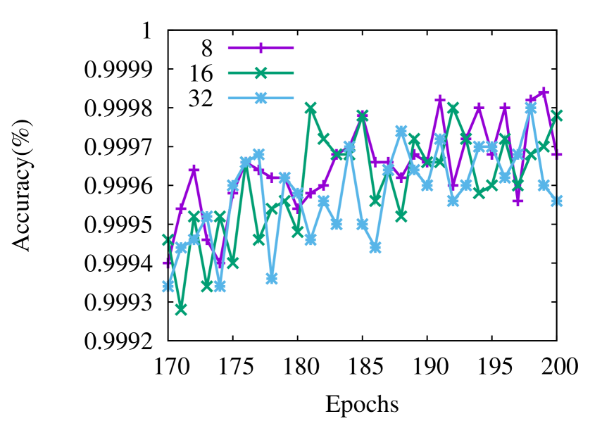
(a) ResNet-18

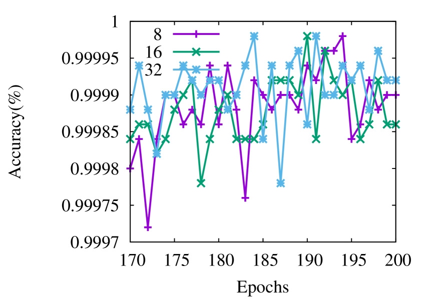
(b) GoogLeNet

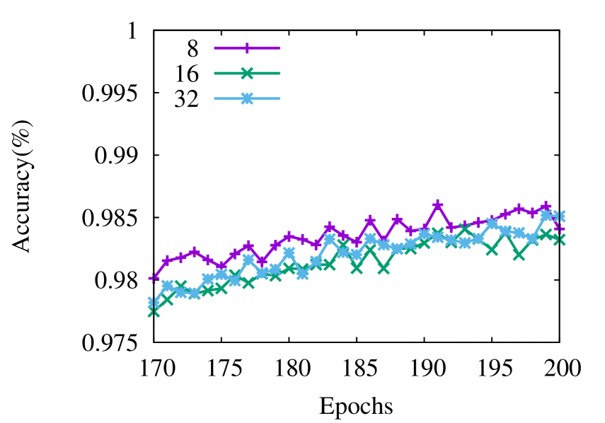
(c) MobileNet

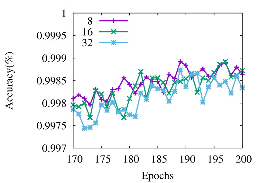
(d) VGG19

Figure 1: Impact of $K_{2}$ on convergence: training accuracy

Modern neural networks are typically fairly deep and have a large number of weights. Without mitigation, overfitting can plague generalization performance. Thus, we also investigate the impact of $K_{2}$ on test accuracy.

Fig. 2(a), 2(b), 2(c) and 2(d) show test accuracies with the same setup for ResNet-18, GoogLeNet, MobileNet, and VGG19 respectively. For ResNet-18, the best test accuracy is achieved with $K_{2}=16$, about 0.3% higher than with $K_{2}=8$. For GoogLeNet, the best test accuracy is achieved with $K_{2}=32$, although at epoch 200 all three runs show similar test accuracy. For MobileNet, $K_{2}=8$, $16$, and $32$ have similar test performance. For VGG19, $K_{2}=8$ has the best test accuracy at epoch 200.

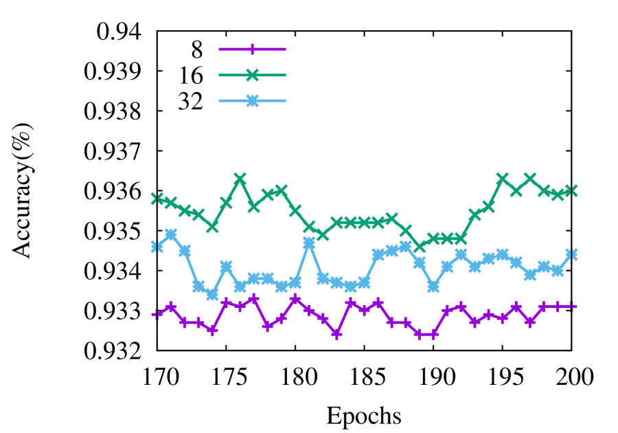
(a) ResNet-18

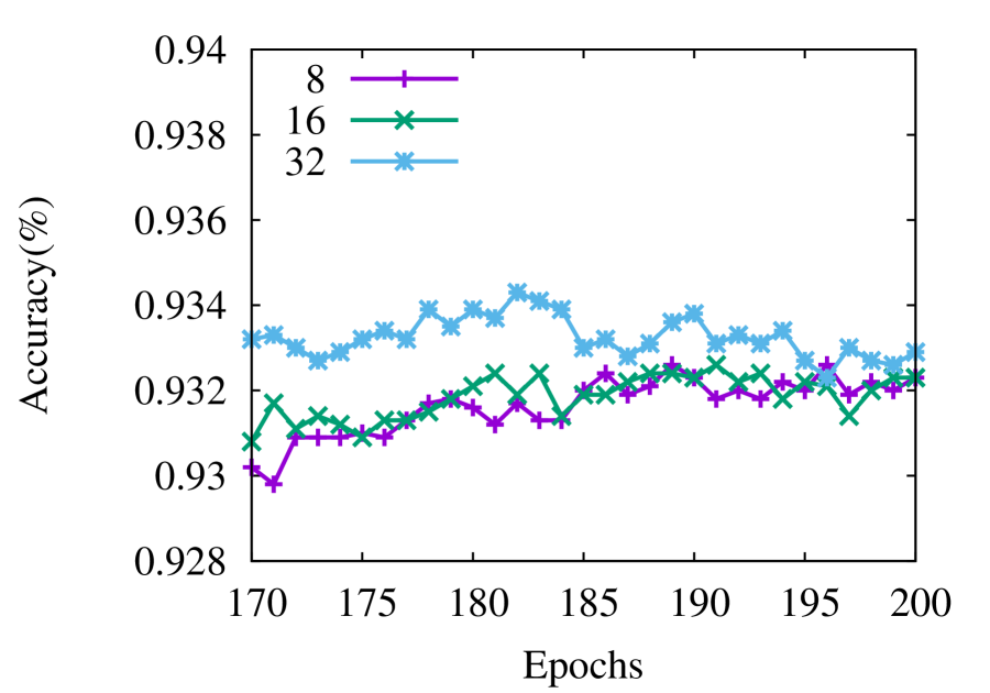
(b) GoogLeNet

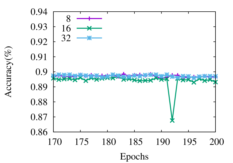
(c) MobileNet

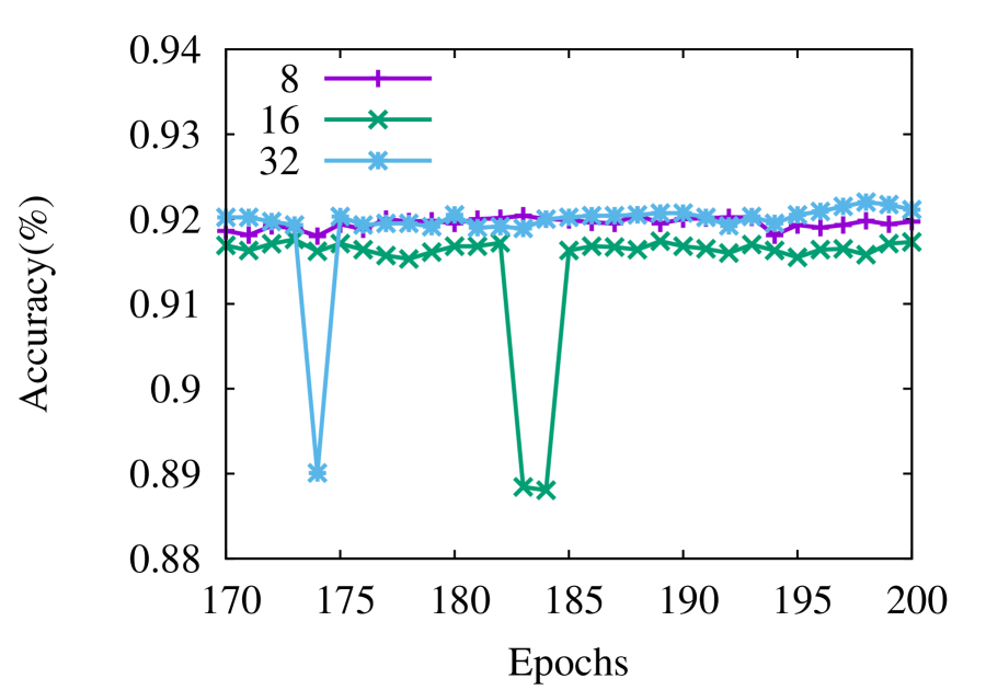
(d) VGG19

Figure 2: Impact of $K_{2}$ on convergence: test accuracy

It is clear that increasing $K_{2}$ does not necessarily reduce convergence speed for training, but obviously it reduces the frequency of costly global reduction when $P$ increases. For example, the best test accuracy for GoogLeNet is achieved with $K_{2}=32$. In comparison with $K_{2}=8$, 4 times fewer global reductions are used. As a result, the real run time for training can be effectively reduced due to much less communication overhead.

4.2 Impact of $K_{1}$ and $S$ on Convergence

In section 3.4, Theorem 3.5 claims that reducing $K_{1}$ and increasing $S$ can speed up training convergence. In practice, with a limited budget in terms of the amount of data samples processed (e.g., a fixed number of training epochs), we can adjust $K_{1}$ and $S$ to accelerate training. Recall that $K_{1}$ and $S$ determine local communication behavior. They provide deterministic means, at least in theory, for practitioners to fine tune training to achieve the best results within their computational budget and time constraint.

Fig. 3(a), 3(b), 3(c) and 3(d) show the impact of $K_{1}$ on convergence. As all networks achieve high training accuracy, we show the evolution of trainig loss from epoch 170 to epoch 200. In each figure we show the training loss for $K_{1}=4$ and $8$, and we set $K_{2}=32$, $S=4$, and $P=16$. As we can see, for all networks it is clear that a lower training loss is achieved with $K_{1}=4$ than with $K_{1}=8$.

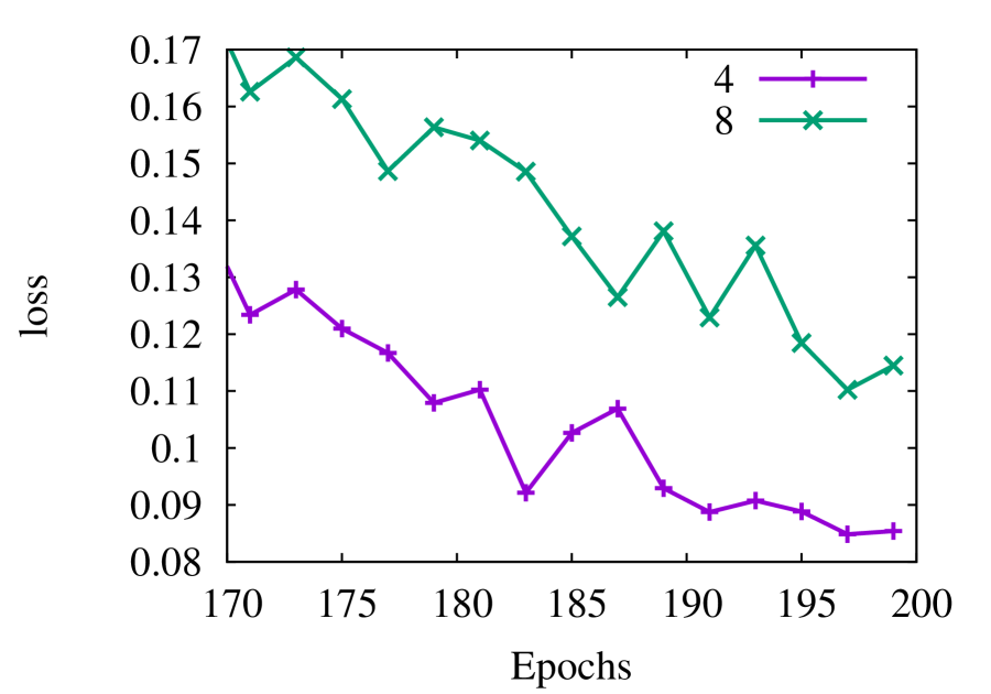
(a) ResNet-18

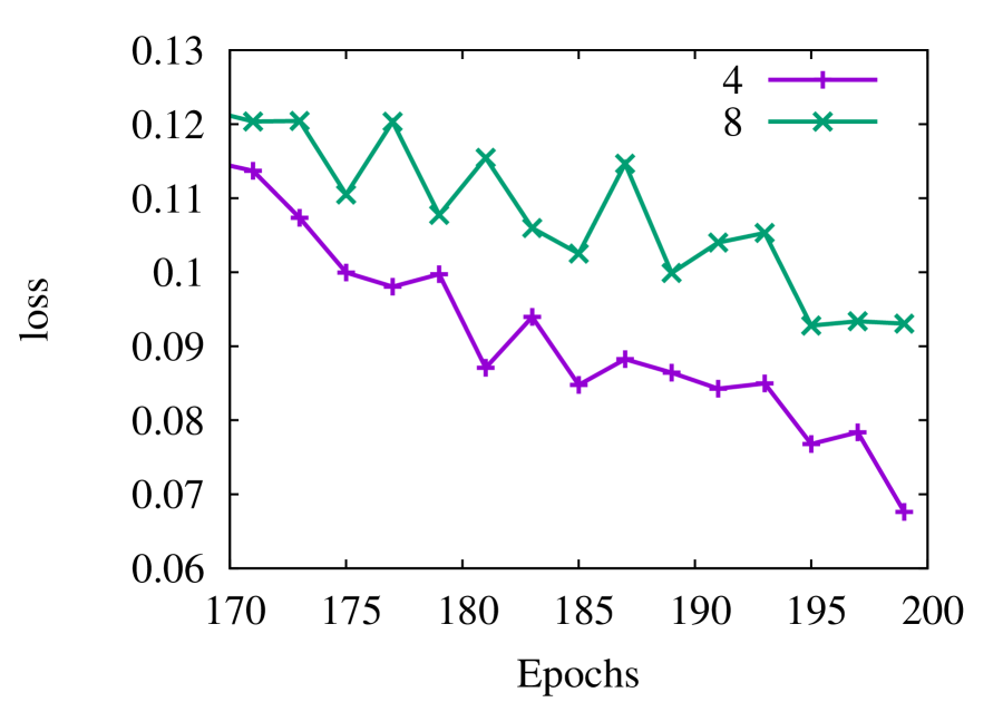
(b) GoogLeNet

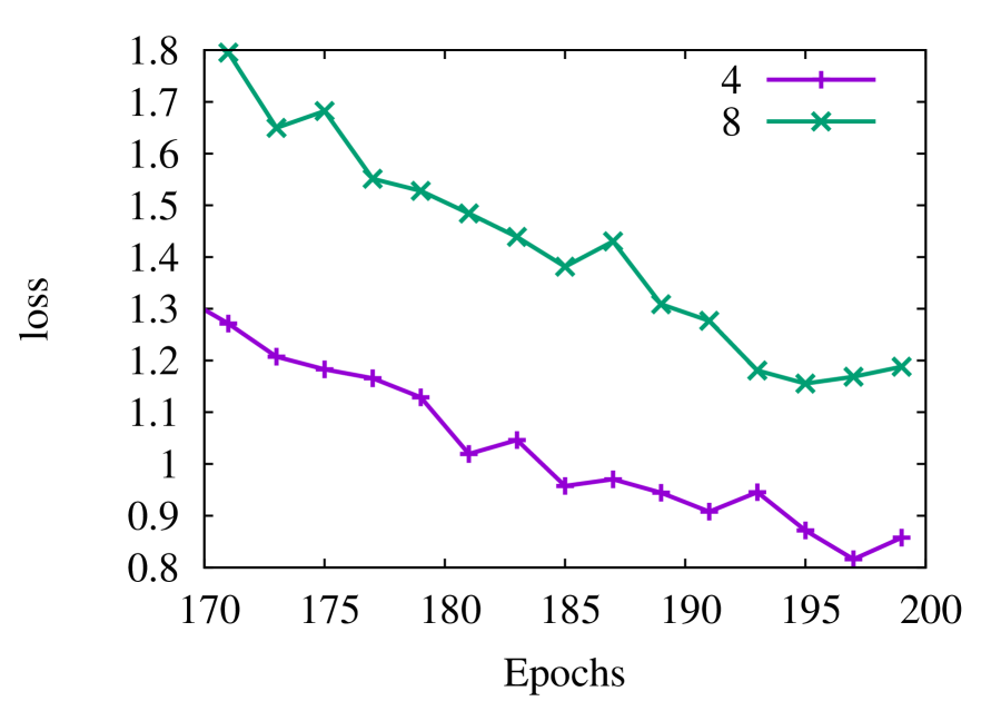
(c) MobileNet

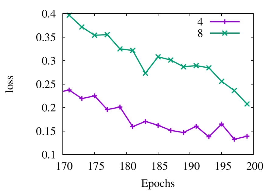
(d) VGG19

Figure 3: Training loss with $K_{1}=4$ and $K_{1}=8$

Fig. 4(a), 4(b), 4(c) and 4(d) show the impact of $S$ on convergence. Again we show the evolution of trainig loss from epoch 170 to epoch 200. In each figure we plot the training loss for $S=2$ and $4$, and we set $K_{2}=32$, $K_{1}=4$, and $P=16$. In all figures lower training loss is achieved with $S=4$ than with $S=2$.

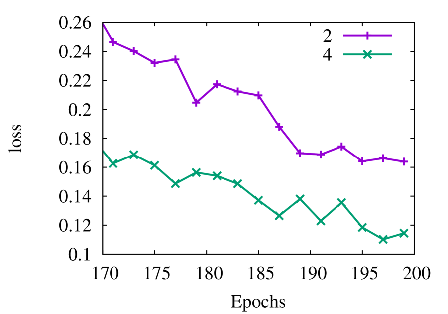
(a) ResNet-18

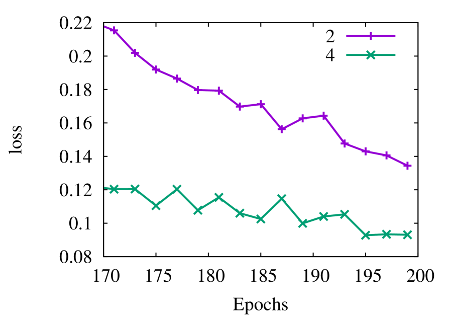
(b) GoogLeNet

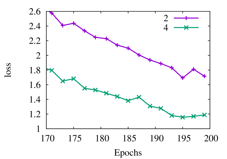
(c) MobileNet

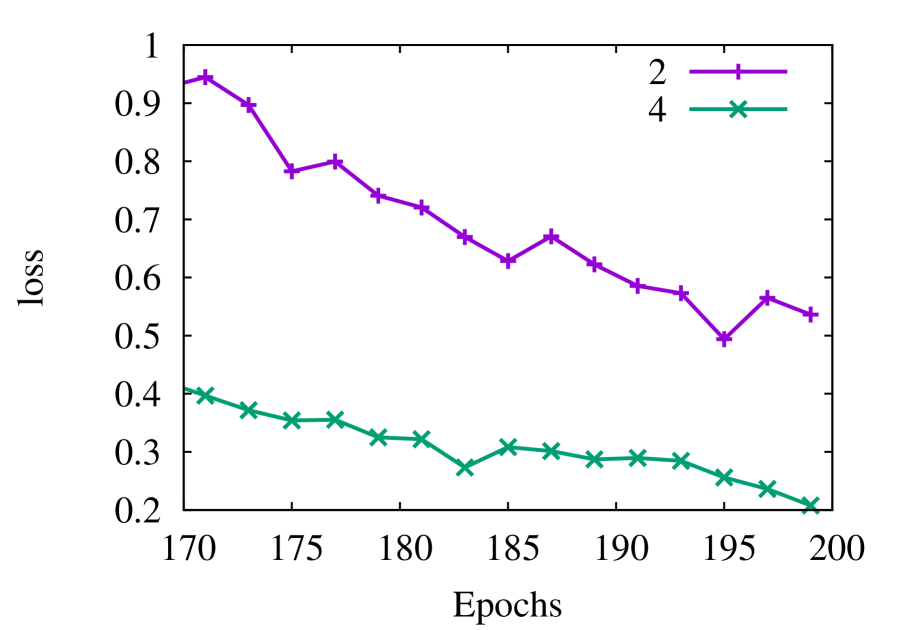
(d) VGG19

Figure 4: Training loss with $S=2$, $4$

4.3 Comparison with K-AVG

As we have mentioned, one of the biggest challenges of distributed training is the communication overhead. In K-AVG, $K$ determines the frequency of global reduction. It is shown by Zhou and Cong (2018), from the perspective of convergence, large $P$ may require small $K$ for faster convergence. We explained in section 3.5 that Hier-AVG provides the option to reduce global reduction frequency by using local averaging. Since modern architectures typically employ multiple GPUs per node, and the intra-node communication bandwidth is much higher than inter-node bandwith, Hier-AVG is a perfect match for such systems.

We evaluate the performance of Hier-AVG by setting $K_{2}=2K_{opt}$ and $S=4$, where $K_{opt}$ is the fine tuned value of $K$ for K-AVG implementation. The experimental results is summarized in Table 1. We experiment with $P=16$, $32$, and $64$ learners on ResNet-18. With $16$ learners, $K_{opt}=32$ for K-AVG. Then we set $K_{2}=64$ for Hier-AVG, and experiment with $K_{1}=2$, $4$, and $16$. The corespoinding validation accuracies are $94.01\%$, $94.11\%$, and $94.08\%$ respectively. They are all higher than the best accuracy achieved by K-AVG at $94.0\%$. With 32 and 64 learners, $K_{opt}=4$ for K-AVG. We set $K_{2}=8$ for Hier-AVG, the accuracies achieved are $93.90\%$ and $93.17\%$ at $K_{1}=4$, $S=8$ and $K_{1}=1$ $S=4$, respectively. The best accuracies achieved by K-AVG with 32 and 64 learners are $93.7\%$ and $92.5\%$ respectively.

In our experiments, while reducing the gobal reduction frequency by half, Hier-AVG still achieves validation accuracy comparable to K-AVG. Note that we do not show the actual wallclock time per epoch because Pytorch implementations do not support GPU-direct communication yet on our target architecture. For all reductions, the data is copied from GPU to CPU first. It is clear though once GPU-direct communication is implemented, Hier-AVG can effectively reduce communication time.

Alg.	$K_{opt}$	$K_{2}$	$K_{1}$	$S$	$P$	Test accuracy
K-AVG	32	-	-	-	16	$94.00\%$
Hier-AVG	-	64	2	4	16	94.01%
Hier-AVG	-	64	4	4	16	94.11%
Hier-AVG	-	64	16	4	16	94.08%
K-AVG	4	-	-	-	32	$93.70\%$
Hier-AVG	-	8	4	8	32	93.90%
K-AVG	4	-	-	-	64	$92.50\%$
Hier-AVG	-	8	1	4	64	93.17%

Table 1: Comparison of Hier-AVG and K-AVG

4.4 Performance of Hier-AVG on ImageNet

In this section, we further investigate the performance of Hier-AVG with the ImageNet-1K dataset which is much larger than CIFAR-10 and it contains of 1.28 million training images split across 1000 classes, and 50,000 validation images.

During training, a crop of random size (of $0.08$ to 1.5) of the original size and a random aspect ratio (of 3/4 to 4/3) of the original aspect ratio is made. This crop is then resized to $224\times 224$. Random color jittering with a ratio of 0.4 to the brightness, contrast and saturation of an image is then applied. Next a random horizontal flip is applied to the input, and the input is then normalized with mean (0.485, 0.456, 0.406) and standard deviation (0.229, 0.224, 0.225) for the (R, G, B) channels respectively. For K-AVG we set $K=43$, and for Hier-AVG we set $K_{2}=43$, $K_{1}=20$, and $S=4$.

Fig. 5(a) shows the training accuracies comparison between K-AVG and Hier-AVG with 16 learners. Clearly, Hier-AVG achieves higher training accuracy than K-AVG since the first epoch. After the first 5 epochs, Hier-AVG achieved $6\%$ higher training accuracy than K-AVG, and at the 46-th epoch, Hier-AVG achieved $17.33\%$ higher training accuracy than K-AVG. At the 90-th epoch, the training accuracy of Hier-AVG is $1.15\%$ higher than K-AVG.

Fig. 5(b) shows the test accuracies comparison between K-AVG and Hier-AVG with $16$ learners. As we can see, Hier-AVG also achieves higher validation accuracy than K-AVG since the first epoch. At epoch 5, Hier-AVG achieved $12\%$ higher accuracy than K-AVG, and at the 90-th epoch, Hier-AVG achieved $0.51\%$ higher accuracy than K-AVG.

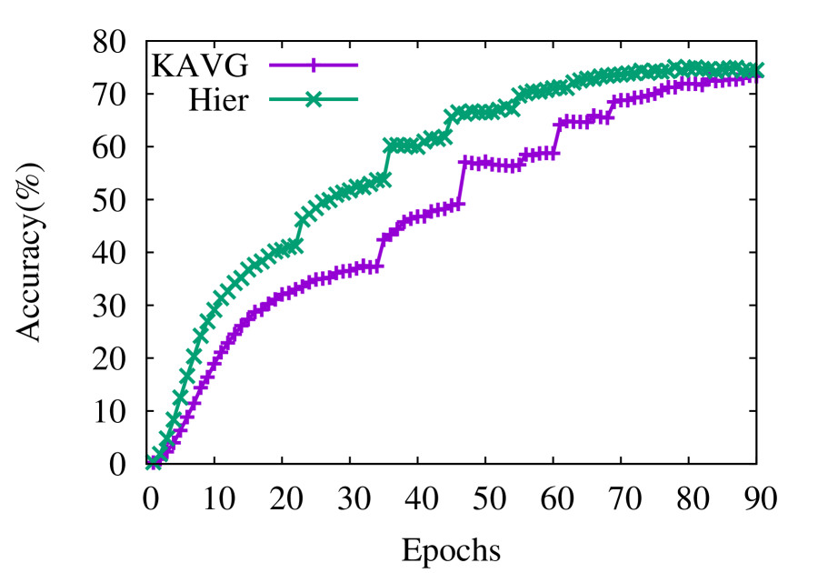
(a) Training

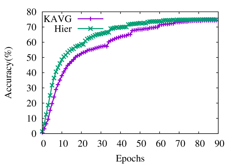
(b) Test

Figure 5: Performance of K-AVG and Hier-AVG with ImageNet-1K

5 Conclusion

We proposed a two stage hierarchical averaging SGD algorithm to effectively reduce communication overhead while not deterioate training and test performance for distributed machine learning. We established the convergence results for Hier-AVG for non-convex optimization problems and show that Hier-AVG with infrequent global reduction can still achieve the expected convergence rate, while oftentimes provides faster training speed and better test accuracy. By introducing local averaging, we show that it can be used to accelerate training. Moreover, we show analytically and experimentally that local averaging can serve as an alternative remedy to reduce global reduction frequency without doing harm to the convergence rate for training and generalization performance for testing. As a result, Hier-AVG provides an alternative method for practitioners to train large scale machine learning applications on distributed platforms.

6 Proofs

6.1 Proof of Theorem 3.1

Proof.

We denote by

$$\bar{\mathbf{w}}_{t}=\frac{1}{P}\sum_{j=1}^{P}\mathbf{w}^{j}_{t}$$ (6.1)

as the global average of local iterates over all $P$ workers. A quick observation is that when $t\equiv 0\mod K_{2}$, then $\bar{\mathbf{w}}_{t}=\widetilde{\mathbf{w}}_{i}$ with $i=t/K_{2}$. In the following theorem, we derive an upper bound on the convergence measured by $T^{-1}\sum^{T}_{t=1}\mathbb{E}\|\nabla F(\bar{\mathbf{w}}_{t-1})\|^{2}_{2}$. It is easy to see that

$$\bar{\mathbf{w}}_{t+1}-\bar{\mathbf{w}}_{t}=-\frac{\gamma}{PB}\sum\limits_{j=1}^{P}\sum\limits_{s=1}^{B}\nabla F(\mathbf{w}_{t}^{j};\xi^{j}_{t+1,s}).$$ (6.2)

Consider

$$\mathbb{E}\Big{[}F(\bar{\mathbf{w}}_{t+1})-F(\bar{\mathbf{w}}_{t})\Big{]} \leq\mathbb{E}\Big{\langle}\nabla F(\bar{\mathbf{w}}_{t}),\bar{\mathbf{w}}_{t+1}-\bar{\mathbf{w}}_{t}\Big{\rangle}+\frac{L}{2}\mathbb{E}\big{\|}\bar{\mathbf{w}}_{t+1}-\bar{\mathbf{w}}_{t}\big{\|}_{2}^{2}$$ (6.3)

$$\leq-\gamma\mathbb{E}\Big{[}\Big{\langle}\nabla F(\bar{\mathbf{w}}_{t}),\frac{1}{P}\sum_{j=1}^{P}\nabla F(\mathbf{w}^{j}_{t})\Big{\rangle}\Big{]}$$ (6.4)

$$+\frac{L\gamma^{2}}{2P^{2}B^{2}}\mathbb{E}\big{\|}\sum\limits_{j=1}^{P}\sum\limits_{s=1}^{B}\nabla F(\mathbf{w}^{j}_{t};\xi^{j}_{t+1,s})\big{\|}_{2}^{2}.$$ (6.5)

where (6.4) is due to the fact that random variables $\nabla F(\mathbf{w}_{t}^{j};\xi^{j}_{t+1,s})$ are i.i.d. over $s$ for fixed $t$ and $j$ conditioning on previous steps. In the following, we will bound (6.4) and (6.5) respectively.

For (6.4), some simple algebra implies that

$$-\gamma\mathbb{E}\Big{[}\Big{\langle}\nabla F(\bar{\mathbf{w}}_{t}),\frac{1}{P}\sum_{j=1}^{P}\nabla F(\mathbf{w}^{j}_{t})\Big{\rangle}\Big{]}$$ (6.6)

$$=-\frac{\gamma}{2}\mathbb{E}\Big{[}\|\nabla F(\bar{\mathbf{w}}_{t})\|_{2}^{2}+\big{\|}\frac{1}{P}\sum_{j=1}^{P}\nabla F(\mathbf{w}_{t}^{j})\big{\|}_{2}^{2}-\big{\|}\nabla F(\bar{\mathbf{w}}_{t})-\frac{1}{P}\sum_{j=1}^{P}\nabla F(\mathbf{w}_{t}^{j})\big{\|}_{2}^{2}\Big{]}$$

For term $\big{\|}\nabla F(\bar{\mathbf{w}}_{t})-\frac{1}{P}\sum_{j=1}^{P}\nabla F(\mathbf{w}_{t}^{j})\big{\|}_{2}^{2}$, we have

$$\mathbb{E}\big{\|}\nabla F(\bar{\mathbf{w}}_{t})-\frac{1}{P}\sum_{j=1}^{P}\nabla F(\mathbf{w}_{t}^{j})\big{\|}_{2}^{2} =\frac{1}{P^{2}}\big{\|}\sum_{j=1}^{P}\Big{(}\nabla F(\bar{\mathbf{w}}_{t})-\nabla F(\mathbf{w}_{t}^{j})\Big{)}\big{\|}_{2}^{2}$$ (6.7)

$$\leq\frac{1}{P}\sum_{j=1}^{P}\mathbb{E}\Big{\|}\nabla F(\bar{\mathbf{w}}_{t})-\nabla F(\mathbf{w}_{t}^{j})\Big{\|}_{2}^{2}$$

$$\leq\frac{L^{2}}{P}\sum_{j=1}^{P}\mathbb{E}\|\bar{\mathbf{w}}_{t}-\mathbf{w}_{t}^{j}\|_{2}^{2}.$$

To bound $\mathbb{E}\|\bar{\mathbf{w}}_{t}-\mathbf{w}_{t}^{j}\|_{2}^{2}$, we first set $t_{0}$ to be the largest integer such that $t_{0}\equiv 0\mod K_{2}$ and $t_{0}\leq t$. In other words, $t_{0}$ is the latest iteration number that is less than $t$ when global averaging happens. Then we can write

$$\mathbf{w}^{j}_{t}=\bar{\mathbf{w}}_{t_{0}}-\frac{\gamma}{B}\sum_{\tau=t_{0}+1}^{t}\sum_{s=1}^{B}\nabla F(\mathbf{w}_{\tau-1}^{j},\xi^{j}_{\tau,s})$$ (6.8)

and

$$\bar{\mathbf{w}}_{t}=\bar{\mathbf{w}}_{t_{0}}-\frac{\gamma}{PB}\sum_{j=1}^{P}\sum_{\tau=t_{0}+1}^{t}\sum_{s=1}^{B}\nabla F(\mathbf{w}_{\tau-1}^{j},\xi^{j}_{\tau,s}).$$ (6.9)

Plug (6.8) and (6.9) in $\mathbb{E}\|\bar{\mathbf{w}}_{t}-\mathbf{w}_{t}^{j}\|_{2}^{2}$, we get

$$\mathbb{E}\big{\|}\bar{\mathbf{w}}_{t}-\mathbf{w}_{t}^{j}\big{\|}_{2}^{2} =\gamma^{2}\mathbb{E}\big{\|}\sum_{\tau=t_{0}+1}^{t}\Big{(}\frac{1}{PB}\sum_{j=1}^{P}\sum_{s=1}^{B}\nabla F(\mathbf{w}_{\tau-1}^{j},\xi^{j}_{\tau,s})-\frac{1}{B}\sum_{s=1}^{B}\nabla F(\mathbf{w}^{j}_{\tau-1},\xi^{j}_{\tau,s})\Big{)}\big{\|}_{2}^{2}$$ (6.10)

$$\leq 2\gamma^{2}\mathbb{E}\Big{(}\big{\|}\sum_{\tau=t_{0}+1}^{t}\frac{1}{PB}\sum_{j=1}^{P}\sum_{s=1}^{B}\nabla F(\mathbf{w}_{\tau-1}^{j},\xi^{j}_{\tau,s})\big{\|}_{2}^{2}+\big{\|}\sum_{\tau=t_{0}+1}^{t}\frac{1}{B}\sum_{s=1}^{B}\nabla F(\mathbf{w}_{\tau-1}^{j},\xi^{j}_{\tau,s})\big{\|}_{2}^{2}\Big{)}$$

$$\leq 2\gamma^{2}(t-t_{0})\sum_{\tau=t_{0}+1}^{t}\sum_{s=1}^{B}\Big{(}\frac{1}{PB}\sum_{j=1}^{P}\mathbb{E}\big{\|}\nabla F(\mathbf{w}_{\tau-1}^{j},\xi^{j}_{\tau,s})\big{\|}_{2}^{2}+\frac{1}{B}\mathbb{E}\big{\|}\nabla F(\mathbf{w}_{\tau-1}^{j},\xi^{j}_{\tau,s})\big{\|}_{2}^{2}\Big{)}$$

$$\leq 4\gamma^{2}(t-t_{0})^{2}M_{G}^{2}$$

$$\leq 4\gamma^{2}K_{2}^{2}M_{G}^{2}.$$

Plug (6.10) back into (6.7), we get

$$\mathbb{E}\big{\|}\nabla F(\bar{\mathbf{w}}_{t})-\frac{1}{P}\sum_{j=1}^{P}\nabla F(\mathbf{w}_{t}^{j})\big{\|}_{2}^{2}\leq 4L^{2}\gamma^{2}K_{2}^{2}M_{G}^{2}.$$ (6.11)

Then we get the bound on (6.4) as

$$-\gamma\mathbb{E}\Big{[}\Big{\langle}\nabla F(\bar{\mathbf{w}}_{t}),\frac{1}{P}\sum_{j=1}^{P}\nabla F(\mathbf{w}^{j}_{t})\Big{\rangle}\Big{]}\leq-\frac{\gamma}{2}\mathbb{E}\Big{[}\|\nabla F(\bar{\mathbf{w}}_{t})\|_{2}^{2}+\big{\|}\frac{1}{P}\sum_{j=1}^{P}\nabla F(\mathbf{w}_{t}^{j})\big{\|}_{2}^{2}\Big{]}+2L^{2}\gamma^{3}K_{2}^{2}M_{G}^{2}.$$ (6.12)

On the other hand, for (6.5) we have

$$\frac{L\gamma^{2}}{2}\mathbb{E}\big{\|}\frac{1}{PB}\sum\limits_{j=1}^{P}\sum\limits_{s=1}^{B}\nabla F(\mathbf{w}^{j}_{t};\xi^{j}_{t+1,s})\big{\|}_{2}^{2}$$ (6.13)

$$\leq\frac{L\gamma^{2}}{2}\mathbb{E}\big{\|}\frac{1}{PB}\sum\limits_{j=1}^{P}\sum\limits_{s=1}^{B}\big{(}\nabla F(\mathbf{w}^{j}_{t};\xi^{j}_{t+1,s})-\nabla F(\mathbf{w}^{j}_{t})+\nabla F(\mathbf{w}^{j}_{t})\big{)}\big{\|}_{2}^{2}$$ (6.14)

$$\leq\frac{L\gamma^{2}}{2}\mathbb{E}\big{\|}\frac{1}{PB}\sum\limits_{j=1}^{P}\sum\limits_{s=1}^{B}\big{(}\nabla F(\mathbf{w}^{j}_{t};\xi^{j}_{t+1,s})-\nabla F(\mathbf{w}^{j}_{t})\big{)}\big{\|}_{2}^{2}+\frac{L\gamma^{2}}{2}\mathbb{E}\big{\|}\frac{1}{P}\sum_{j=1}^{P}\nabla F(\mathbf{w}^{j}_{t})\big{\|}_{2}^{2}$$ (6.15)

$$\leq\frac{L\gamma^{2}}{2P^{2}B^{2}}\sum\limits_{j=1}^{P}\sum\limits_{s=1}^{B}\mathbb{E}\big{\|}\nabla F(\mathbf{w}^{j}_{t};\xi^{j}_{t+1,s})-\nabla F(\mathbf{w}^{j}_{t})\big{\|}_{2}^{2}+\frac{L\gamma^{2}}{2}\mathbb{E}\big{\|}\frac{1}{P}\sum_{j=1}^{P}\nabla F(\mathbf{w}^{j}_{t})\big{\|}_{2}^{2}$$ (6.16)

$$\leq\frac{L\gamma^{2}M}{2PB}+\frac{L\gamma^{2}}{2}\mathbb{E}\big{\|}\frac{1}{P}\sum_{j=1}^{P}\nabla F(\mathbf{w}^{j}_{t})\big{\|}_{2}^{2}$$ (6.17)

where (6.15) is due to $P^{-1}\mathbb{E}\sum_{j=1}^{P}\big{(}\nabla F(\mathbf{w}^{j}_{t};\xi^{j}_{t+1,s})-\nabla F(\mathbf{w}^{j}_{t})\big{)}=0$ condition on $\mathbf{w}_{t}^{j}$ and the independence over $s$. (6.16) is due to the same trick and conditional independence over $j$ and $s$.

Combine (6.12) and (6.17), we get

$$\mathbb{E}\Big{[}F(\bar{\mathbf{w}}_{t+1})-F(\bar{\mathbf{w}}_{t})\Big{]}\leq-\frac{\gamma}{2}\mathbb{E}\|\nabla F(\bar{\mathbf{w}}_{t})\|_{2}^{2}-\frac{\gamma(1-L\gamma)}{2}\big{\|}\frac{1}{P}\sum_{j=1}^{P}\nabla F(\mathbf{w}_{t}^{j})\big{\|}_{2}^{2}+2L^{2}\gamma^{3}K_{2}^{2}M_{G}^{2}+\frac{L\gamma^{2}M}{2PB}.$$

Take the summation over $t$, under the assumption $0<L\gamma\leq 1$ we get

$$\frac{\gamma}{2}\sum_{t=0}^{T-1}\mathbb{E}\big{\|}\nabla F(\bar{\mathbf{w}}_{t})\big{\|}_{2}^{2}\leq\Big{[}F(\bar{\mathbf{w}}_{0})-\mathbb{E}F(\bar{\mathbf{w}}_{T})\Big{]}+2L^{2}\gamma^{3}K_{2}^{2}M_{G}^{2}+\frac{L\gamma^{2}M}{2PB},$$ (6.18)

which leads to

$$\frac{1}{T}\sum_{t=0}^{T-1}\mathbb{E}\big{\|}\nabla F(\bar{\mathbf{w}}_{t})\big{\|}_{2}^{2} \leq\frac{2(F(\bar{\mathbf{w}}_{0})-\mathbb{E}F(\bar{\mathbf{w}}_{T}))}{\gamma T}+4L^{2}\gamma^{2}K_{2}^{2}M_{G}^{2}+\frac{L\gamma M}{PB}$$ (6.19)

$$\leq\frac{2(F(\bar{\mathbf{w}}_{0})-F^{*}}{\gamma T}+4L^{2}\gamma^{2}K_{2}^{2}M_{G}^{2}+\frac{L\gamma M}{PB}$$

By setting $\gamma=\sqrt{PB/T}$ and $K_{2}=T^{1/4}/(PB)^{3/4}$, we get

$$\frac{1}{T}\sum_{t=0}^{T-1}\mathbb{E}\big{\|}\nabla F(\bar{\mathbf{w}}_{t})\big{\|}_{2}^{2}\leq\frac{2(F(\bar{\mathbf{w}}_{0})-F^{*})}{\sqrt{PBT}}+\frac{4L^{2}M_{G}^{2}}{\sqrt{PBT}}+\frac{LM}{\sqrt{PBT}}.$$ (6.20)

∎

6.2 Proof of Theorem 3.2

Proof.

We denote $\tilde{w}_{n}$ as the $n$-th global update in Hier-AVG, denote $\bar{\mathbf{w}}^{j}_{n+kK_{1}+t}$ as $t$-th local update on learner $j$ after $k$ times local averaging. By the algorithm,

$$\widetilde{\mathbf{w}}_{n+1}-\widetilde{\mathbf{w}}_{n}=-\frac{\gamma}{PB}\sum\limits_{j=1}^{P}\sum\limits_{k=0}^{\beta-1}\sum\limits_{t=0}^{K_{1}-1}\sum\limits_{s=1}^{B}\nabla F(\bar{\mathbf{w}}_{n+kK_{1}+t}^{j};\xi^{j}_{kK_{1}+t,s}).$$

By the definition of SGD, the random variables $\xi^{j}_{kK_{1}+t,s}$ are i.i.d. for all $t=0,...,K_{1}-1$, $s=1,...,B$, $j=1,...,P$ and $k=0,...,\beta-1$.

Consider

$$\mathbb{E}\Big{[}F(\widetilde{\mathbf{w}}_{n+1})-F(\widetilde{\mathbf{w}}_{n})\Big{]} \leq\mathbb{E}\Big{\langle}\nabla F(\widetilde{\mathbf{w}}_{n}),\widetilde{\mathbf{w}}_{n+1}-\widetilde{\mathbf{w}}_{n}\Big{\rangle}+\frac{L}{2}\mathbb{E}\big{\|}\widetilde{\mathbf{w}}_{n+1}-\widetilde{\mathbf{w}}_{n}\big{\|}_{2}^{2}$$ (6.21)

$$\leq-\gamma\Big{\langle}\nabla F(\widetilde{\mathbf{w}}_{n}),\mathbb{E}\sum\limits_{k=0}^{\beta-1}\sum\limits_{t=0}^{K_{1}-1}\nabla F(\bar{\mathbf{w}}^{j}_{n+kK_{1}+t})\Big{\rangle}$$ (6.22)

$$+\frac{L\gamma^{2}}{2P^{2}B^{2}}\mathbb{E}\big{\|}\sum\limits_{j=1}^{P}\sum\limits_{k=0}^{\beta-1}\sum\limits_{t=0}^{K_{1}-1}\sum\limits_{s=1}^{B}\nabla F(\bar{\mathbf{w}}^{j}_{n+kK_{1}+t};\xi^{j}_{kK_{1}+t,s})\big{\|}_{2}^{2}.$$ (6.23)

Note that here we abused the expectation notation $\mathbb{E}$ a little bit. Throughout this proof, $\mathbb{E}$ always means taking the overall expectation. For each fixed $k$ and $t$, the random variables $\nabla F(\bar{\mathbf{w}}_{n+kK_{1}+t}^{j};\xi^{j}_{kK_{1}+t,s})$ are i.i.d. for over all $j$ and $s$ conditioning on previous steps. As a result, we can drop the summation over $s$ and $j$ in (6.22) due to the averaging factors $B$ and $P$ in the dominator. To be more specific, under the unbiasness Assumption 3, by taking the overall expectation we can immediately get

$$\mathbb{E}\frac{1}{B}\sum\limits_{s=1}^{B}\nabla F(\bar{\mathbf{w}}_{\alpha+t}^{j};\xi_{\alpha+t,s}^{j})=\mathbb{E}\Big{[}\frac{1}{B}\sum\limits_{s=1}^{B}\mathbb{E}_{\xi^{j}_{t,s}}\nabla F(\bar{\mathbf{w}}_{\alpha+t}^{j};\xi_{t,s}^{j}|\bar{\mathbf{w}}_{\alpha+t}^{j})\Big{]}=\mathbb{E}\nabla F(\bar{\mathbf{w}}_{\alpha+t}^{j}).$$

for fixed $j$ and $t$. Next, we show how to get rid of the summation over $j$. Recall that $\bar{\mathbf{w}}^{j}_{\alpha+1}=\bar{\mathbf{w}}_{\alpha}-\frac{\gamma}{B}\sum_{s=1}^{B}\nabla F(\bar{\mathbf{w}}_{\alpha};\xi^{j}_{0,s})$. Obviously, $\bar{\mathbf{w}}_{\alpha+1}^{j}$, $j=1,...,P$ are i.i.d. condiitoning on $\bar{\mathbf{w}}_{\alpha}$ because $\xi_{0,s}^{j}$, $j=1,...,P$, $s=1,...,B$ are i.i.d. Similarly, $\bar{\mathbf{w}}^{j}_{\alpha+2}=\bar{\mathbf{w}}^{j}_{\alpha+1}-\frac{\gamma}{B}\sum_{s=1}^{B}\nabla F(\bar{\mathbf{w}}^{j}_{\alpha+1};\xi^{j}_{1,s})$, $j=1,...,P$ are i.i.d. due to the fact that $\bar{\mathbf{w}}_{\alpha+t}^{j}$’s are i.i.d., $\xi_{1,s}^{j}$’s are i.i.d., and $\bar{\mathbf{w}}_{\alpha+t}^{j}$’s are independent from $\xi_{1,s}^{j}$’s. By induction, one can easily show that for each fixed $t$, $\bar{\mathbf{w}}_{\alpha+t}^{j}$, $j=1,...,P$ are i.i.d. Thus for each fixed $t$

$$\frac{1}{P}\sum\limits_{j=1}^{P}\mathbb{E}\nabla F(\bar{\mathbf{w}}_{\alpha+t}^{j})=\mathbb{E}\nabla F(\bar{\mathbf{w}}_{\alpha+t}^{j}).$$

We can therefore get rid of the summation over $j$ as well. We will frequently use the above iterative conditional expectation trick in the following analysis.

Next, we will bound (6.22) and (6.23) respectively. For (6.23), we have

$$\frac{L\gamma^{2}K_{1}\beta}{2P^{2}B^{2}}\mathbb{E}\sum\limits_{k=0}^{\beta-1}\sum\limits_{t=0}^{K_{1}-1}\big{\|}\sum\limits_{j=1}^{P}\sum\limits_{s=1}^{B}\nabla F(\bar{\mathbf{w}}^{j}_{n+kK_{1}+t};\xi^{j}_{kK_{1}+t,s})\big{\|}_{2}^{2}$$

$$=\frac{L\gamma^{2}K_{1}\beta}{2P^{2}B^{2}}\mathbb{E}\sum\limits_{k=0}^{\beta-1}\sum\limits_{t=0}^{K_{1}-1}\big{\|}\sum\limits_{j=1}^{P}\sum\limits_{s=1}^{B}\big{(}\nabla F(\bar{\mathbf{w}}^{j}_{n+kK_{1}+t};\xi^{j}_{kK_{1}+t,s})-\nabla F(\bar{\mathbf{w}}^{j}_{n+kK_{1}+t})+\nabla F(\bar{\mathbf{w}}^{j}_{n+kK_{1}+t})\big{)}\big{\|}_{2}^{2}$$

$$=\frac{L\gamma^{2}K_{1}\beta}{2P^{2}B^{2}}\mathbb{E}\sum\limits_{k=0}^{\beta-1}\sum\limits_{t=0}^{K_{1}-1}\big{\|}\sum\limits_{j=1}^{P}\sum\limits_{s=1}^{B}\big{(}\nabla F(\bar{\mathbf{w}}^{j}_{n+kK_{1}+t};\xi^{j}_{kK_{1}+t,s})-\nabla F(\bar{\mathbf{w}}^{j}_{n+kK_{1}+t})\big{)}\big{\|}_{2}^{2}$$

$$+\frac{L\gamma^{2}K_{1}\beta}{2P^{2}B^{2}}\mathbb{E}\sum\limits_{k=0}^{\beta-1}\sum\limits_{t=0}^{K_{1}-1}\big{\|}\sum\limits_{j=1}^{P}\sum\limits_{s=1}^{B}\nabla F(\bar{\mathbf{w}}^{j}_{n+kK_{1}+t})\big{\|}_{2}^{2}$$

$$+\frac{L\gamma^{2}K_{1}\beta}{P^{2}B^{2}}\sum\limits_{k=0}^{\beta-1}\sum\limits_{t=0}^{K_{1}-1}\mathbb{E}\Big{\langle}\sum\limits_{j=1}^{P}\sum\limits_{s=1}^{B}\big{(}\nabla F(\bar{\mathbf{w}}^{j}_{n+kK_{1}+t};\xi^{j}_{kK_{1}+t,s})-\nabla F(\bar{\mathbf{w}}^{j}_{n+kK_{1}+t})\big{)},\sum\limits_{j=1}^{P}\sum\limits_{s=1}^{B}\nabla F(\bar{\mathbf{w}}^{j}_{n+kK_{1}+t})\Big{\rangle}$$

$$=\frac{L\gamma^{2}K_{1}\beta}{2P^{2}B^{2}}\mathbb{E}\sum\limits_{k=0}^{\beta-1}\sum\limits_{t=0}^{K_{1}-1}\big{\|}\sum\limits_{j=1}^{P}\sum\limits_{s=1}^{B}\big{(}\nabla F(\bar{\mathbf{w}}^{j}_{n+kK_{1}+t};\xi^{j}_{kK_{1}+t,s})-\nabla F(\bar{\mathbf{w}}^{j}_{n+kK_{1}+t})\big{)}\big{\|}_{2}^{2}$$

$$+\frac{L\gamma^{2}K_{1}\beta}{2P^{2}B^{2}}\mathbb{E}\sum\limits_{k=0}^{\beta-1}\sum\limits_{t=0}^{K_{1}-1}\big{\|}\sum\limits_{j=1}^{P}\sum\limits_{s=1}^{B}\nabla F(\bar{\mathbf{w}}^{j}_{n+kK_{1}+t})\big{\|}_{2}^{2},$$

where in the last equity, we used the fact that for fixed $t$ and $k$ and conditioning on $\nabla F(\bar{\mathbf{w}}^{j}_{n+kK_{1}+t})$, $\sum\limits_{j=1}^{P}\sum\limits_{s=1}^{B}\mathbb{E}\big{(}\nabla F(\bar{\mathbf{w}}^{j}_{n+kK_{1}+t};\xi^{j}_{kK_{1}+t,s})-\nabla F(\bar{\mathbf{w}}^{j}_{n+kK_{1}+t})\big{)}=0$ under unbiasness Assumption 3. Further, under the bounded variance Assumption 4, we have

$$\frac{L\gamma^{2}K_{1}\beta}{2P^{2}B^{2}}\mathbb{E}\sum\limits_{k=0}^{\beta-1}\sum\limits_{t=0}^{K_{1}-1}\big{\|}\sum\limits_{j=1}^{P}\sum\limits_{s=1}^{B}\nabla F(\bar{\mathbf{w}}^{j}_{n+kK_{1}+t};\xi^{j}_{kK_{1}+t,s})\big{\|}_{2}^{2}$$

$$=\frac{L\gamma^{2}K_{1}\beta}{2P^{2}B^{2}}\mathbb{E}\sum\limits_{k=0}^{\beta-1}\sum\limits_{t=0}^{K_{1}-1}\sum\limits_{j=1}^{P}\sum\limits_{s=1}^{B}\mathbb{E}\big{\|}\nabla F(\bar{\mathbf{w}}^{j}_{n+kK_{1}+t};\xi^{j}_{kK_{1}+t,s})-\nabla F(\bar{\mathbf{w}}^{j}_{n+kK_{1}+t})\big{\|}_{2}^{2}$$

$$+\frac{L\gamma^{2}K_{1}\beta}{2}\sum\limits_{k=0}^{\beta-1}\sum\limits_{t=0}^{K_{1}-1}\mathbb{E}\big{\|}\nabla F(\bar{\mathbf{w}}^{j}_{n+kK_{1}+t})\big{\|}_{2}^{2}$$

$$\leq\frac{L\gamma^{2}K_{1}^{2}\beta^{2}M}{2PB}+\frac{L\gamma^{2}K_{1}\beta}{2}\sum\limits_{k=0}^{\beta-1}\sum\limits_{t=0}^{K_{1}-1}\mathbb{E}\big{\|}\nabla F(\bar{\mathbf{w}}^{j}_{n+kK_{1}+t})\big{\|}_{2}^{2}.$$

Thus, we get

$$\frac{L\gamma^{2}}{2P^{2}B^{2}}\mathbb{E}\big{\|}\sum\limits_{j=1}^{P}\sum\limits_{k=0}^{\beta-1}\sum\limits_{t=0}^{K_{1}-1}\sum\limits_{s=1}^{B}\nabla F(\bar{\mathbf{w}}^{j}_{n+kK_{1}+t};\xi^{j}_{kK_{1}+t,s})\big{\|}_{2}^{2}$$

$$\leq\frac{L\gamma^{2}K_{1}^{2}\beta^{2}M}{2PB}+\frac{L\gamma^{2}K_{1}\beta}{2}\sum\limits_{k=0}^{\beta-1}\sum\limits_{t=0}^{K_{1}-1}\mathbb{E}\big{\|}\nabla F(\bar{\mathbf{w}}^{j}_{n+kK_{1}+t})\big{\|}_{2}^{2}.$$

Note that in the first equity we can change the summation over $j$ and $s$ out of the squared norms without introducing an extra $PB$ factor is due to the fact that conditioning on $\bar{\mathbf{w}}^{j}_{n+kK_{1}+t}$, $\nabla F(\bar{\mathbf{w}}^{j}_{n+kK_{1}+t};\xi^{j}_{kK_{1}+t,s})$ are all independent with respect to different $j$ and $s$. In the following, we will use this trick over and over again without further explaination.

For (6.22), we have

$$-\gamma\Big{\langle}F(\widetilde{\mathbf{w}}_{n}),\mathbb{E}\sum\limits_{k=0}^{\beta-1}\sum\limits_{t=0}^{K_{1}-1}\nabla F(\bar{\mathbf{w}}^{j}_{n+kK_{1}+t})\Big{\rangle}$$ (6.24)

$$=-\frac{\gamma}{2}\sum\limits_{k=0}^{\beta-1}\sum\limits_{t=0}^{K_{1}-1}\Big{(}\mathbb{E}\big{\|}\nabla F(\widetilde{\mathbf{w}}_{n})\big{\|}_{2}^{2}+\mathbb{E}\big{\|}\nabla F(\bar{\mathbf{w}}_{n+kK_{1}+t}^{j})\big{\|}_{2}^{2}\Big{)}+\frac{\gamma}{2}\sum\limits_{k=0}^{\beta-1}\sum\limits_{t=0}^{K_{1}-1}\mathbb{E}\big{\|}\nabla F(\bar{\mathbf{w}}_{n+kK_{1}+t}^{j})-\nabla F(\widetilde{\mathbf{w}}_{n})\big{\|}_{2}^{2}$$

$$\leq-\frac{\gamma\beta K_{1}}{2}\mathbb{E}\big{\|}\nabla F(\widetilde{\mathbf{w}}_{n})\big{\|}_{2}^{2}-\frac{\gamma}{2}\sum\limits_{k=0}^{\beta-1}\sum\limits_{t=0}^{K_{1}-1}\mathbb{E}\big{\|}\nabla F(\bar{\mathbf{w}}^{j}_{n+kK_{1}+t})\big{\|}_{2}^{2}+\frac{\gamma L^{2}}{2}\sum\limits_{k=0}^{\beta-1}\sum\limits_{t=0}^{K_{1}-1}\mathbb{E}\big{\|}\bar{\mathbf{w}}_{n+kK_{1}+t}^{j}-\widetilde{\mathbf{w}}_{n}\big{\|}_{2}^{2},$$

where we used the Lipschitz Assumption 1 in the last inequality.

In the following lemma, we derive a general bound on $\mathbb{E}\big{\|}\bar{\mathbf{w}}_{n+kK_{1}+t}^{j}-\widetilde{\mathbf{w}}_{n}\big{\|}_{2}^{2}$.

Lemma 1.

For any $t\in\{0,1,2,...,K_{1}-1\}$ and $\eta\in\{0,1,2,...,\beta-1\}$, we have

$$\mathbb{E}\big{\|}\bar{\mathbf{w}}_{n+kK_{1}+t}^{j}-\widetilde{\mathbf{w}}_{n}\big{\|}_{2}^{2}\leq\frac{\gamma^{2}M}{B}(K_{1}\eta+t)\Big{(}t+\frac{K_{1}\eta}{S}\Big{)}+\gamma^{2}(K_{1}\eta+t)\sum\limits_{k=0}^{K_{1}\eta+t}\mathbb{E}\Big{\|}\nabla F(\bar{\mathbf{w}}_{n+k}^{j})\Big{\|}_{2}^{2}$$ (6.25)

Proof.

Recall that for any $P_{j}$ in a local cluster $P_{lc}$ with $|P_{lc}|=S$,

$$\bar{\mathbf{w}}_{n+kK_{1}+t}^{j}-\widetilde{\mathbf{w}}_{n}$$

$$=\frac{\gamma}{BS}\sum\limits_{j\in P_{lc}}\sum\limits_{\eta=0}^{k-1}\sum\limits_{r=0}^{K_{1}-1}\sum\limits_{s=1}^{B}\nabla F(\bar{\mathbf{w}}_{n+\eta K_{1}+r}^{j};\xi_{\eta K_{1}+r,s}^{j})+\frac{\gamma}{B}\sum\limits_{i=0}^{t-1}\sum\limits_{s=1}^{B}\nabla F(\bar{\mathbf{w}}_{n+kK_{1}+i}^{j};\xi_{\eta K_{1}+i,s}^{j}).$$

Therefore,

$$\mathbb{E}\big{\|}\bar{\mathbf{w}}_{n+\eta K_{1}+t}^{j}-\widetilde{\mathbf{w}}_{n}\big{\|}_{2}^{2}$$ (6.26)

$$=\mathbb{E}\Big{\|}\sum\limits_{i=0}^{t-1}\frac{\gamma}{B}\sum\limits_{s=1}^{B}\nabla F(\bar{\mathbf{w}}_{n+\eta K_{1}+i}^{j};\xi_{n+\eta K_{1}+i,s}^{j})+\frac{\gamma}{BS}\sum\limits_{j\in P_{lc}}\sum\limits_{k=0}^{\eta-1}\sum\limits_{r=0}^{K_{1}-1}\sum\limits_{s=1}^{B}\nabla F(\bar{\mathbf{w}}_{n+kK_{1}+r}^{j};\xi_{n+kK_{1}+r,s}^{j})\Big{\|}_{2}^{2}$$ (6.27)

$$\leq\frac{\gamma^{2}}{B^{2}}(K_{1}\eta+t)\sum\limits_{i=0}^{t-1}\mathbb{E}\big{\|}\sum\limits_{s=1}^{B}\nabla F(\bar{\mathbf{w}}_{n+\eta K_{1}+i}^{j};\xi_{n+\eta K_{1}+i,s}^{j})\big{\|}_{2}^{2}$$ (6.28)

$$+\frac{\gamma^{2}}{B^{2}S^{2}}(K_{1}\eta+t)\sum\limits_{k=0}^{\eta-1}\sum\limits_{r=0}^{K_{1}-1}\mathbb{E}\big{\|}\sum\limits_{j\in P_{lc}}\sum\limits_{s=1}^{B}\nabla F(\bar{\mathbf{w}}_{n+kK_{1}+r}^{j};\xi_{kK_{1}+r,s}^{j})\big{\|}_{2}^{2}$$ (6.29)

For term (6.28)

$$\frac{\gamma^{2}}{B^{2}}(K_{1}\eta+t)\sum\limits_{i=0}^{t-1}\mathbb{E}\big{\|}\sum\limits_{s=1}^{B}\nabla F(\bar{\mathbf{w}}_{n+\eta K_{1}+i}^{j};\xi_{n+\eta K_{1}+i,s}^{j})\big{\|}_{2}^{2}$$ (6.30)

$$=\frac{\gamma^{2}}{B^{2}}(K_{1}\eta+t)\sum\limits_{i=0}^{t-1}\mathbb{E}\big{\|}\sum\limits_{s=1}^{B}\Big{(}\nabla F(\bar{\mathbf{w}}_{n+\eta K_{1}+i}^{j};;\xi_{n+\eta K_{1}+i,s}^{j})-\nabla F(\bar{\mathbf{w}}_{n+\eta K_{1}+i}^{j})+\nabla F(\bar{\mathbf{w}}_{n+\eta K_{1}+i}^{j})\Big{)}\big{\|}_{2}^{2}$$ (6.31)

$$\leq\frac{\gamma^{2}}{B^{2}}(K_{1}\eta+t)\sum\limits_{i=0}^{t-1}\sum\limits_{s=1}^{B}\mathbb{E}\Big{\|}\nabla F(\bar{\mathbf{w}}_{n+\eta K_{1}+i}^{j};;\xi_{n+\eta K_{1}+i,s}^{j})-\nabla F(\bar{\mathbf{w}}_{n+\eta K_{1}+i}^{j})\Big{\|}_{2}^{2}$$ (6.32)

$$+\gamma^{2}(K_{1}\eta+t)\sum\limits_{i=0}^{t-1}\mathbb{E}\Big{\|}\nabla F(\bar{\mathbf{w}}_{n+\eta K_{1}+i}^{j})\Big{\|}_{2}^{2}$$ (6.33)

$$\leq\frac{\gamma^{2}M}{B}(K_{1}\eta+t)t+\gamma^{2}(K_{1}\eta+t)\sum\limits_{i=0}^{t-1}\mathbb{E}\Big{\|}\nabla F(\bar{\mathbf{w}}_{n+\eta K_{1}+i}^{j})\Big{\|}_{2}^{2}.$$ (6.34)

Similarly, for term (6.29) we have

$$\frac{\gamma^{2}}{B^{2}S^{2}}(K_{1}\eta+t)\sum\limits_{k=0}^{\eta-1}\sum\limits_{r=0}^{K_{1}-1}\mathbb{E}\big{\|}\sum\limits_{j\in P_{lc}}\sum\limits_{s=1}^{B}\nabla F(\bar{\mathbf{w}}_{n+kK_{1}+r}^{j};\xi_{kK_{1}+r,s}^{j})\big{\|}_{2}^{2}$$ (6.35)

$$\leq\frac{\gamma^{2}M}{BS}(K_{1}\eta+t)K_{1}\eta+\gamma^{2}(K_{1}\eta+t)\sum\limits_{k=0}^{\eta-1}\sum\limits_{r=0}^{K_{1}-1}\mathbb{E}\Big{\|}\nabla F(\bar{\mathbf{w}}_{n+kK_{1}+r}^{j})\Big{\|}_{2}^{2}.$$ (6.36)

Combine (6.34) and (6.36), we get

$$\mathbb{E}\big{\|}\bar{\mathbf{w}}_{n+\eta K_{1}+t}^{j}-\widetilde{\mathbf{w}}_{n}\big{\|}_{2}^{2}\leq\frac{\gamma^{2}M}{B}(K_{1}\eta+t)\Big{(}t+\frac{K_{1}\eta}{S}\Big{)}+\gamma^{2}(K_{1}\eta+t)\sum\limits_{k=0}^{K_{1}\eta+t-1}\mathbb{E}\Big{\|}\nabla F(\bar{\mathbf{w}}_{n+k}^{j})\Big{\|}_{2}^{2}.$$

∎

Therefore, using the result of Lemma 1

$$\frac{\gamma L^{2}}{2}\sum\limits_{\eta=0}^{\beta-1}\sum\limits_{t=0}^{K_{1}-1}\mathbb{E}\big{\|}\bar{\mathbf{w}}_{n+\eta K_{1}+t}^{j}-\widetilde{\mathbf{w}}_{n}\big{\|}_{2}^{2}$$

$$\leq\frac{L^{2}\gamma^{3}M}{2B}\sum\limits_{\eta=0}^{\beta-1}\sum\limits_{t=0}^{K_{1}-1}(K_{1}\eta+t)\Big{(}t+\frac{K_{1}\eta}{S}\Big{)}+\frac{L^{2}\gamma^{3}M}{2}\sum\limits_{\eta=0}^{\beta-1}\sum\limits_{t=0}^{K_{1}-1}(K_{1}\eta+t)\sum\limits_{k=0}^{K_{1}\eta+t-1}\mathbb{E}\Big{\|}\nabla F(\bar{\mathbf{w}}_{n+k}^{j})\Big{\|}_{2}^{2}$$

$$=\frac{L^{2}\gamma^{3}MK_{2}}{24B}\Big{(}\frac{(K_{2}-K_{1})(4K_{2}+K_{1}-3)}{S}+(K_{1}-1)(3K_{2}+K_{1}-2)\Big{)}$$

$$+\frac{L^{2}\gamma^{3}MK_{2}(K_{2}-1)}{2}\mathbb{E}\Big{\|}\nabla F(\tilde{\mathbf{w}}_{n})\Big{\|}_{2}^{2}$$

$$+\frac{L^{2}\gamma^{3}M}{2}\sum\limits_{\eta=0}^{\beta-1}\sum\limits_{t=0}^{K_{1}-1}(K_{1}\eta+t)\mathbf{1}\{K_{1}\eta+t-1\geq 1\}\sum\limits_{k=1}^{K_{1}\eta+t-1}\mathbb{E}\Big{\|}\nabla F(\bar{\mathbf{w}}_{n+k}^{j})\Big{\|}_{2}^{2}.$$

Then we will have an upper bound on $\sum\limits_{\eta=0}^{\beta-1}\sum\limits_{t=0}^{K_{1}-1}(K_{1}\eta+t)\mathbf{1}\{K_{1}\eta+t-1\geq 1\}\sum\limits_{k=1}^{K_{1}\eta+t-1}\mathbb{E}\Big{\|}\nabla F(\bar{\mathbf{w}}_{n+k}^{j})\Big{\|}_{2}^{2}$.

Lemma 2.

$$\sum\limits_{\eta=0}^{\beta-1}\sum\limits_{t=0}^{K_{1}-1}(K_{1}\eta+t)\mathbf{1}\{K_{1}\eta+t-1\geq 1\}\sum\limits_{k=1}^{K_{1}\eta+t-1}\mathbb{E}\Big{\|}\nabla F(\bar{\mathbf{w}}_{n+k}^{j})\Big{\|}_{2}^{2}$$ (6.37)

$$\leq\Big{(}\frac{K_{2}(K_{2}-1)}{2}-1-\delta_{\nabla F,\mathbf{w}}\Big{)}\sum\limits_{k=1}^{K_{2}-1}\mathbb{E}\Big{\|}\nabla F(\bar{\mathbf{w}}^{j}_{n+k})\Big{\|}_{2}^{2},$$

where $\delta\in(0,K_{2}(K_{2}-3)/2)$ is a constant depending on the immediate gradient norms $\|\nabla F(\bar{\mathbf{w}}^{j}_{n+k})\|_{2}^{2}$, $k=1,...,K_{2}-1$.

Proof.

Obviously, $\mathbb{E}\Big{\|}\nabla F(\bar{\mathbf{w}}_{n+1}^{j})\Big{\|}_{2}^{2}$ has the most copies, we will derive an upper bound on the number of $\mathbb{E}\Big{\|}\nabla F(\bar{\mathbf{w}}_{n+1}^{j})\Big{\|}_{2}^{2}$ and then use this bound to uniformly bound the number of terms for $\mathbb{E}\Big{\|}\nabla F(\bar{\mathbf{w}}_{n+k}^{j})\Big{\|}_{2}^{2}$, $k=1,...,K_{2}-2$.

$$\sum\limits_{\eta=0}^{\beta-1}\sum\limits_{t=0}^{K_{1}-1}(K_{1}\eta+t)\mathbf{1}\{K_{1}\eta+t-1\geq 1\}$$

$$\leq\sum\limits_{t=0}^{K_{1}-1}t\mathbf{1}\{t\geq 2\}\mathbf{1}\{K_{1}\geq 3\}+\sum\limits_{t=0}^{K_{1}-1}(K_{1}+t)\mathbf{1}\{K_{1}+t\geq 2\}\mathbf{1}\{K_{1}\geq 2\}$$

$$+\sum\limits_{\eta=2}^{\beta-1}\sum\limits_{t=0}^{K_{1}-1}(K_{1}\eta+t)\mathbf{1}\{K_{1}\eta+t\geq 2\}$$

$$=\frac{(K_{1}-2)(K_{1}+1)}{2}\mathbf{1}\{K_{1}\geq 3\}+\frac{K_{1}(3K_{1}-1)}{2}\mathbf{1}\{K_{1}\geq 2\}+\frac{(K_{2}-2K_{1})(K_{2}+2K_{1}-1)}{2}$$

$$\leq\frac{K_{2}(K_{2}-1)}{2}-1.$$

∎

Following Lemma 2, we get

$$\frac{\gamma L^{2}}{2}\sum\limits_{\eta=0}^{\beta-1}\sum\limits_{t=0}^{K_{1}-1}\mathbb{E}\big{\|}\bar{\mathbf{w}}_{n+\eta K_{1}+t}^{j}-\widetilde{\mathbf{w}}_{n}\big{\|}_{2}^{2}$$ (6.38)

$$<\frac{L^{2}\gamma^{3}MK_{2}}{24B}\Big{(}\frac{(K_{2}-K_{1})(4K_{2}+K_{1}-3)}{S}+(K_{1}-1)(3K_{2}+K_{1}-2)\Big{)}$$

$$+\frac{L^{2}\gamma^{3}MK_{2}(K_{2}-1)}{2}\mathbb{E}\Big{\|}\nabla F(\tilde{\mathbf{w}}_{n})\Big{\|}_{2}^{2}$$

$$+\frac{L^{2}\gamma^{3}}{2}\Big{(}\frac{K_{2}(K_{2}-1)}{2}-1-\delta_{\nabla F,\mathbf{w}}\Big{)}\sum\limits_{k=1}^{K_{2}-1}\mathbb{E}\Big{\|}\nabla F(\bar{\mathbf{w}}^{j}_{n+k})\Big{\|}_{2}^{2}.$$

Plug (6.38) into (LABEL:bias), we have

$$-\gamma\Big{\langle}F(\widetilde{\mathbf{w}}_{n}),\mathbb{E}\sum\limits_{k=0}^{\beta-1}\sum\limits_{t=0}^{K_{1}-1}\nabla F(\bar{\mathbf{w}}^{j}_{n+kK_{1}+t})\Big{\rangle}$$ (6.39)

$$\leq-\frac{\gamma(K_{2}+1)}{2}\Big{[}1-\frac{L^{2}\gamma^{2}K_{2}(K_{2}-1)}{2(K_{2}+1)}\Big{]}\mathbb{E}\big{\|}\nabla F(\widetilde{\mathbf{w}}_{n})\big{\|}_{2}^{2}$$

$$-\frac{\gamma}{2}\Big{(}1-L^{2}\gamma^{2}\Big{(}\frac{K_{2}(K_{2}-1)}{2}-1-\delta_{\nabla F,\mathbf{w}}\Big{)}\sum\limits_{k=1}^{K_{2}-1}\mathbb{E}\Big{\|}\nabla F(\bar{\mathbf{w}}^{j}_{n+k})\Big{\|}_{2}^{2}$$

$$+\frac{L^{2}\gamma^{3}MK_{2}}{24B}\Big{(}\frac{(K_{2}-K_{1})(4K_{2}+K_{1}-3)}{S}+(K_{1}-1)(3K_{2}+K_{1}-2)\Big{)}$$

Plug (6.23) and (LABEL:bias_final) back into $\mathbb{E}\Big{[}F(\widetilde{\mathbf{w}}_{n+1})-F(\widetilde{\mathbf{w}}_{n})\Big{]}$, we get

$$\mathbb{E}\Big{[}F(\widetilde{\mathbf{w}}_{n+1})-F(\widetilde{\mathbf{w}}_{n})\Big{]}$$ (6.40)

$$\leq-\frac{\gamma(K_{2}+1)}{2}\Big{[}1-\frac{L^{2}\gamma^{2}(K_{2}-1)K_{2}}{2(K_{2}+1)}-\frac{L\gamma K_{2}}{K_{2}+1}\Big{]}\mathbb{E}\big{\|}\nabla F(\widetilde{\mathbf{w}}_{n})\big{\|}_{2}^{2}$$

$$-\frac{\gamma}{2}\Big{(}1-L^{2}\gamma^{2}\Big{(}\frac{K_{2}(K_{2}-1)}{2}-1-\delta_{\nabla F,\mathbf{w}}\Big{)}-L\gamma K_{2}\Big{)}\sum\limits_{k=1}^{K_{2}-1}\mathbb{E}\Big{\|}\nabla F(\bar{\mathbf{w}}^{j}_{n+k})\Big{\|}_{2}^{2}$$

$$+\frac{L^{2}\gamma^{3}MK_{2}}{24B}\Big{(}\frac{(K_{2}-K_{1})(4K_{2}+K_{1}-3)}{S}+(K_{1}-1)(3K_{2}+K_{1}-2)\Big{)}+\frac{L\gamma^{2}K_{2}^{2}M}{2PB}$$

Under the condition,

$$1-L^{2}\gamma^{2}\Big{(}\frac{K_{2}(K_{2}-1)}{2}-1-\delta_{\nabla F,\mathbf{w}}\Big{)}-L\gamma K_{2}\geq 0,$$

we have

$$\frac{\gamma(K_{2}+1)}{2}\Big{[}1-\frac{L^{2}\gamma^{2}(K_{2}-1)K_{2}}{2(K_{2}+1)}-\frac{L\gamma K_{2}}{K_{2}+1}\Big{]}\geq\frac{\gamma}{2}\Big{(}K_{2}-L^{2}\gamma^{2}(1+\delta_{\nabla F,\mathbf{w}})\Big{)}.$$

We can therefore drop the second term on the right hand side in (6.40) and take the summation over $n$ to get

$$\mathbb{E}\Big{[}F(\widetilde{\mathbf{w}}_{N})-F(\widetilde{\mathbf{w}}_{1})\Big{]}$$ (6.41)

$$\leq-\frac{\gamma}{2}\Big{(}K_{2}-L^{2}\gamma^{2}(1+\delta_{\nabla F,\mathbf{w}})\Big{)}\sum\limits_{n=1}^{N}\mathbb{E}\big{\|}\nabla F(\widetilde{\mathbf{w}}_{n})\big{\|}_{2}^{2}$$

$$+\frac{L^{2}\gamma^{3}MK_{2}}{24B}\Big{(}\frac{(K_{2}-K_{1})(4K_{2}+K_{1}-3)}{S}+(K_{1}-1)(3K_{2}+K_{1}-2)\Big{)}+\frac{L\gamma^{2}K_{2}^{2}M}{2PB}$$

Under Assumption 2, we have

$$F^{*}-F(\widetilde{\mathbf{w}}_{1})\leq F(\widetilde{\mathbf{w}}_{N})-F(\widetilde{\mathbf{w}}_{1}).$$ (6.42)

As a result,

$$\frac{\gamma}{2}\Big{(}K_{2}-L^{2}\gamma^{2}(1+\delta_{\nabla F,\mathbf{w}})\Big{)}\sum\limits_{n=1}^{N}\mathbb{E}\big{\|}\nabla F(\widetilde{\mathbf{w}}_{n})\big{\|}_{2}^{2}$$

$$\leq\mathbb{E}\Big{[}F(\widetilde{\mathbf{w}}_{1})-F^{*}\Big{]}+\frac{L^{2}\gamma^{3}MK_{2}}{24B}\Big{(}\frac{(K_{2}-K_{1})(4K_{2}+K_{1}-3)}{S}+(K_{1}-1)(3K_{2}+K_{1}-2)\Big{)}+\frac{L\gamma^{2}K_{2}^{2}M}{2PB}$$

Thus we have

$$\frac{1}{N}\sum\limits_{n=1}^{N}\mathbb{E}\big{\|}\nabla F(\widetilde{\mathbf{w}}_{n})\big{\|}_{2}^{2}\leq\frac{2\mathbb{E}[F(\widetilde{\mathbf{w}}_{1})-F^{*}]}{N[K_{2}-L^{2}\gamma^{2}(1+\delta_{\nabla F,\mathbf{w}})]\gamma}+\frac{L\gamma MK_{2}^{2}}{PB[K_{2}-L^{2}\gamma^{2}(1+\delta_{\nabla F,\mathbf{w}})]}$$

$$+\frac{L^{2}\gamma^{2}MK_{2}}{12B[K_{2}-L^{2}\gamma^{2}(1+\delta_{\nabla F,\mathbf{w}})]}\Big{(}\frac{(K_{2}-K_{1})(4K_{2}+K_{1}-3)}{S}+(K_{1}-1)(3K_{2}+K_{1}-2)\Big{)}.$$

∎

6.3 Proof of Theorem 3.3

Proof.

The proof of Theorem 3.3 is similar to that of Theorem 3.2. Indeed, under the condition (3.5),

$$1-L^{2}\gamma^{2}_{j}\Big{(}\frac{K_{2}(K_{2}-1)}{2}-1-\delta_{\nabla F,\mathbf{w}}\Big{)}-L\gamma_{j}K_{2}\geq 0,$$

we have

$$\frac{\gamma_{j}(K_{2}+1)}{2}\Big{[}1-\frac{L^{2}\gamma_{j}^{2}K_{2}(K_{2}-1)}{2(K_{2}+1)}-\frac{L\gamma_{j}K_{2}}{K_{2}+1}\Big{]}\geq\frac{\gamma_{j}}{2}\Big{(}K_{2}-L^{2}\gamma_{j}^{2}(1+\delta_{\nabla F,\mathbf{w}})\Big{)}.$$ (6.43)

Meanwhile, from (6.3), we have $L^{2}\gamma_{j}^{2}(1+\delta_{\nabla F,\mathbf{w}})\leq L^{2}\gamma_{j}^{2}K_{2}^{2}/2\leq 1$, thus $K_{2}-L^{2}\gamma_{j}^{2}(1+\delta_{\nabla F,\mathbf{w}})\geq K_{2}-1$. By replacing $\gamma$ with $\gamma_{j}$ in (6.40) together with (6.43), we have

$$\frac{\gamma_{j}(K_{2}-1)}{2}\mathbb{E}\big{\|}\nabla F(\widetilde{\mathbf{w}}_{j})\big{\|}_{2}^{2}\leq\mathbb{E}\Big{[}F(\widetilde{\mathbf{w}}_{j+1})-F(\widetilde{\mathbf{w}}_{j})\Big{]}$$ (6.44)

$$+\frac{L\gamma_{j}^{2}K_{2}^{2}M}{2PB}+\frac{L^{2}\gamma_{j}^{3}MK_{2}}{24B}\Big{(}\frac{(K_{2}-K_{1})(4K_{2}+K_{1}-3)}{S}+(K_{1}-1)(3K_{2}+K_{1}-2)\Big{)}$$

Taking the summation over $j$, and divide both sides by $\sum_{j=1}^{N}\gamma_{j}$, we got

$$\mathbb{E}\sum\limits_{j=1}^{N}\frac{\gamma_{j}}{\sum_{j=1}^{N}\gamma_{j}}\big{\|}\nabla F(\widetilde{\mathbf{w}}_{j})\big{\|}_{2}^{2}\leq\frac{2\mathbb{E}[F(\widetilde{\mathbf{w}}_{1})-F^{*}]}{(K_{2}-1)\sum_{j=1}^{N}\gamma_{j}}+\sum\limits_{j=1}^{N}\frac{LMK_{2}^{2}\gamma_{j}^{2}}{PB_{j}(K_{2}-1)\sum_{j=1}^{N}\gamma_{j}}$$

$$+\sum\limits_{j=1}^{N}\frac{L^{2}MK_{2}\gamma^{3}_{j}}{12B_{j}(K_{2}-1)\sum_{j=1}^{N}\gamma_{j}}\Big{(}\frac{(K_{2}-K_{1})(4K_{2}+K_{1}-3)}{S}+(K_{1}-1)(3K_{2}+K_{1}-2)\Big{)}.$$

∎

6.4 Proof of Theorem 3.4

Proof.

Under the assumption $T=N*K_{2}$, we can rewrite the bound (3.6) as

$$\frac{1}{N}\sum\limits_{n=1}^{N}\mathbb{E}\big{\|}\nabla F(\widetilde{\mathbf{w}}_{n})\big{\|}_{2}^{2}\leq\frac{2\mathbb{E}[F(\widetilde{\mathbf{w}}_{1})-F^{*}]K_{2}}{T(K_{2}-\delta)\gamma}+\frac{L\gamma MK_{2}^{2}}{PB(K_{2}-\delta)}$$

$$+\frac{L^{2}\gamma^{2}MK_{2}}{12B(K_{2}-\delta)}\Big{(}\frac{(K_{2}-K_{1})(4K_{2}+K_{1}-3)}{S}+(K_{1}-1)(3K_{2}+K_{1}-2)\Big{)}$$

To move on, we set

$$B(K_{2}):=f(K_{2})*g(K_{2})$$

where

$$f(K_{2}):=\Big{(}\alpha+\beta K_{2}+\eta\Big{(}\frac{(K_{2}-K_{1})(4K_{2}+K_{1}-3)}{S}+(K_{1}-1)(3K_{2}+K_{1}-2)\Big{)}\Big{)}$$

and

$$g(K_{2}):=\Big{(}\frac{K_{2}}{K_{2}-\delta}\Big{)},~{}\alpha=\frac{2[\mathbb{E}F(\widetilde{\mathbf{w}}_{1})-F^{*}]}{T\gamma},~{}\beta=\frac{L\gamma M}{PB},~{}\eta=\frac{L^{2}\gamma^{2}M}{12B}.$$

To minimize the right hand side of (3.6), it is equivalent to solve the following integer program

$$K_{2}^{*}=\min\limits_{K_{2}\in\mathbb{N}^{*}}B(K_{2}),$$

which can be very hard. Meanwhile, one should notice that $K_{2}^{*}$ depends on some unknown quantities such as $L$, $M$ and $(F(\widetilde{\mathbf{w}}_{1})-F^{*})$. Instead, we investigate the monotonicity of $B(K_{2})$. Firstly, we show that $f(K_{2})$ is non-decreasing.

Lemma 3.

Given $K_{2}\geq K_{1}\geq 1$, $f(K_{2})$ is non-decreasing.

Proof.

The key is to show that $(K_{2}-K_{1})(4K_{2}+K_{1}-3)/S$ is non-decreasing with respect to $K_{2}$. It is easy to see that the quadratic function $(K_{2}-K_{1})(4K_{2}+K_{1}-3)/S$ is non-decreasing with respect to $K_{2}$ when $K_{2}\geq 3(K_{1}+1)/8$, which is always true given $K_{2}\geq K_{1}\geq 1$. Thus, $(K_{2}-K_{1})(4K_{2}+K_{1}-3)/S$ is monotone increasing, so is $f(K_{2})$. ∎

On the other hand, $g(K_{2})$ is monotone decreasing for $K_{2}\geq 1$. Therefore, $B(K_{2})$ is a multiplication of an increasing function and a decreasing one. Thus, a sufficient condition for $K_{2}^{*}>1$ is that $B(2)<B(1)$, which is equivalent to

$$\frac{\delta\alpha}{1-\delta}>2\beta+\frac{12\eta}{S}.$$

∎

6.5 Proof of Theorem 3.5

Proof.

The proof of part 2 is obvious, so we omit it here. For part 1, With $K_{2}$ fixed, it is sufficient to consider the monotonicity of $(K_{2}-K_{1})(4K_{2}+K_{1}-3)/S+(K_{1}-1)(3K_{2}+K_{1}-2)$ for both bounds in (3.6) and (3.8). Set

$$f(K_{1})=\frac{(K_{2}-K_{1})(4K_{2}+K_{1}-3)}{S}+(K_{1}-1)(3K_{2}+K_{1}-2).$$ (6.45)

Then

$$f^{\prime}(K_{1})=\frac{(S-1)(3K_{2}+2K_{1}-3)}{S}.$$

Apparently, $f(K_{1})$ is monotone increasing with respect to $K_{1}$ when $K_{1}\geq 2$ given $S>1$ and $K_{2}\geq K_{1}$. ∎

6.6 Proof of Theorem 3.6

Proof.

When $P$ is large enough such that $L\gamma P\gg 1$, the second term in bound (3.6) is dominanted by the third term. We omit the second term in (3.6) and denote it by $\mathcal{H}(K)$ and get

$$\mathcal{H}(K):=f_{1}(K)*g_{1}(K)$$

where

$$f_{1}(K):=\Big{(}\alpha+\eta\Big{(}\frac{\big{(}(1+a)K-1\big{)}\big{(}2(1+a)K-1\big{)}}{4}\Big{)}$$

and

$$g_{1}(K):=\Big{(}\frac{(1+a)K}{(1+a)K-\delta}\Big{)},~{}\alpha=\frac{2[\mathbb{E}F(\widetilde{\mathbf{w}}_{1})-F^{*}]}{T\gamma},~{}\eta=\frac{L^{2}\gamma^{2}M}{6B}.$$

On the other hand, we denote the similar bound of K-AVG as $\chi(K)$ by plugging in $K_{2}=K$, $K_{1}=1$, $S=1$ in (3.2) (also see Zhou and Cong (2018)), which is

$$\chi(K):=f_{2}(K)*g_{2}(K),$$ (6.46)

where

$$f_{2}(K):=\alpha+\eta(K-1)(2K-1),~{}~{}g_{2}(K):=\Big{(}\frac{K}{K-\delta}\Big{)}.$$

In the following, we show that $\mathcal{H}(K)<\chi(K)$ uniformly for all $K\geq 2$ and $a\in[0,0.443]$. It is easy to see that $0<g_{1}(K)<g_{2}(K)$ for all $K\geq 2$. Next, we show that $f_{1}(K)<f_{2}(K)$ for all $K\geq 2$ and $a\in[0,0.443]$. Set

$$F(K):=f_{1}(K)-f_{2}(K).$$ (6.47)

Then $F(K)$ is a quadratic function of $K$,

$$F^{\prime}(K)=((1+a)^{2}-4)K+3-\frac{3(1+a)}{4},$$ (6.48)

Then it is easy to see that for all $a\in[0,0.779]$ and $F^{\prime}(K)\leq 0$ for all $K\geq 2$. Meanwhile,

$$F(2)=2(1+a)^{2}-\frac{3}{2}(1+a)-\frac{11}{4},$$ (6.49)

and it is easy to check that $F(2)<0$ for all $a\in[0,0.606]$. As a result, $F(K)<0$ for all $K\geq 2$ and $a\in[0,0.606]$. This implies that $\mathcal{H}(K)<\chi(K)$ for all $K\geq 2$ and all $a\in[0,0.606]$.

∎

References

- Bottou et al. [2018] Léon Bottou, Frank E Curtis, and Jorge Nocedal. Optimization methods for large-scale machine learning. SIAM Review, 60(2):223–311, 2018.
- Chen et al. [2016] Jianmin Chen, Xinghao Pan, Rajat Monga, Samy Bengio, and Rafal Jozefowicz. Revisiting distributed synchronous sgd. arXiv preprint arXiv:1604.00981, 2016.
- Dean et al. [2012] Jeffrey Dean, Greg Corrado, Rajat Monga, Kai Chen, Matthieu Devin, Mark Mao, Andrew Senior, Paul Tucker, Ke Yang, Quoc V Le, et al. Large scale distributed deep networks. In Advances in neural information processing systems, pages 1223–1231, 2012.
- Dekel et al. [2012] Ofer Dekel, Ran Gilad-Bachrach, Ohad Shamir, and Lin Xiao. Optimal distributed online prediction using mini-batches. Journal of Machine Learning Research, 13(Jan):165–202, 2012.
- Deng et al. [2009] J. Deng, W. Dong, R. Socher, L.-J. Li, K. Li, and L. Fei-Fei. ImageNet: A Large-Scale Hierarchical Image Database. In CVPR09, 2009.
- Ghadimi and Lan [2013] Saeed Ghadimi and Guanghui Lan. Stochastic first-and zeroth-order methods for nonconvex stochastic programming. SIAM Journal on Optimization, 23(4):2341–2368, 2013.
- Hazan and Kale [2014] Elad Hazan and Satyen Kale. Beyond the regret minimization barrier: optimal algorithms for stochastic strongly-convex optimization. The Journal of Machine Learning Research, 15(1):2489–2512, 2014.
- He et al. [2016] Kaiming He, Xiangyu Zhang, Shaoqing Ren, and Jian Sun. Deep residual learning for image recognition. In Proceedings of the IEEE conference on computer vision and pattern recognition, pages 770–778, 2016.
- Howard et al. [2017] Andrew G Howard, Menglong Zhu, Bo Chen, Dmitry Kalenichenko, Weijun Wang, Tobias Weyand, Marco Andreetto, and Hartwig Adam. Mobilenets: Efficient convolutional neural networks for mobile vision applications. arXiv preprint arXiv:1704.04861, 2017.
- Johnson and Zhang [2013] Rie Johnson and Tong Zhang. Accelerating stochastic gradient descent using predictive variance reduction. In Advances in neural information processing systems, pages 315–323, 2013.
- Krizhevsky and Hinton [2009] Alex Krizhevsky and Geoffrey Hinton. Learning multiple layers of features from tiny images. 2009.
- Li et al. [2014] Mu Li, David G Andersen, Jun Woo Park, Alexander J Smola, Amr Ahmed, Vanja Josifovski, James Long, Eugene J Shekita, and Bor-Yiing Su. Scaling distributed machine learning with the parameter server. In OSDI, volume 1, page 3, 2014.
- Lin et al. [2018] Tao Lin, Sebastian U Stich, and Martin Jaggi. Don’t use large mini-batches, use local sgd. arXiv preprint arXiv:1808.07217, 2018.
- Loshchilov and Hutter [2016] Ilya Loshchilov and Frank Hutter. Sgdr: stochastic gradient descent with restarts. Learning, 10:3, 2016.
- Recht et al. [2011] Benjamin Recht, Christopher Re, Stephen Wright, and Feng Niu. Hogwild: A lock-free approach to parallelizing stochastic gradient descent. In Advances in neural information processing systems, pages 693–701, 2011.
- Robbins and Monro [1951] Herbert Robbins and Sutton Monro. A stochastic approximation method. The annals of mathematical statistics, pages 400–407, 1951.
- Simonyan and Zisserman [2014] Karen Simonyan and Andrew Zisserman. Very deep convolutional networks for large-scale image recognition. arXiv preprint arXiv:1409.1556, 2014.
- Smith et al. [2016] Virginia Smith, Simone Forte, Chenxin Ma, Martin Takác, Michael I Jordan, and Martin Jaggi. Cocoa: A general framework for communication-efficient distributed optimization. arXiv preprint arXiv:1611.02189, 2016.
- Stich [2018] Sebastian U Stich. Local sgd converges fast and communicates little. arXiv preprint arXiv:1805.09767, 2018.
- Szegedy et al. [2015] Christian Szegedy, Wei Liu, Yangqing Jia, Pierre Sermanet, Scott Reed, Dragomir Anguelov, Dumitru Erhan, Vincent Vanhoucke, and Andrew Rabinovich. Going deeper with convolutions. In Proceedings of the IEEE conference on computer vision and pattern recognition, pages 1–9, 2015.
- Wang et al. [2017] Jialei Wang, Weiran Wang, and Nathan Srebro. Memory and communication efficient distributed stochastic optimization with minibatch prox. arXiv preprint arXiv:1702.06269, 2017.
- Wang and Joshi [2018] Jianyu Wang and Gauri Joshi. Adaptive communication strategies to achieve the best error-runtime trade-off in local-update sgd. arXiv preprint arXiv:1810.08313, 2018.
- Yu et al. [2018] Hao Yu, Sen Yang, and Shenghuo Zhu. Parallel restarted sgd for non-convex optimization with faster convergence and less communication. arXiv preprint arXiv:1807.06629, 2018.
- Zhang et al. [2016] Jian Zhang, Christopher De Sa, Ioannis Mitliagkas, and Christopher Ré. Parallel sgd: When does averaging help? arXiv preprint arXiv:1606.07365, 2016.
- Zhou and Cong [2018] Fan Zhou and Guojing Cong. On the convergence properties of a k-step averaging stochastic gradient descent algorithm for nonconvex optimization. In Proceedings of the Twenty-Seventh International Joint Conference on Artificial Intelligence, IJCAI-18, pages 3219–3227, 2018.
- Zinkevich et al. [2010] Martin Zinkevich, Markus Weimer, Lihong Li, and Alex J Smola. Parallelized stochastic gradient descent. In Advances in neural information processing systems, pages 2595–2603, 2010.