Fully Discrete Mixed Finite Element Methods for the Stochastic Cahn-Hilliard Equation with Gradient-type Multiplicative Noise

Abstract

This paper develops and analyzes some fully discrete mixed finite element methods for the stochastic Cahn-Hilliard equation with gradient-type multiplicative noise that is white in time and correlated in space. The stochastic Cahn-Hilliard equation is formally derived as a phase field formulation of the stochastically perturbed Hele-Shaw flow. The main result of this paper is to prove strong convergence with optimal rates for the proposed mixed finite element methods. To overcome the difficulty caused by the low regularity in time of the solution to the stochastic Cahn-Hilliard equation, the Hölder continuity in time with respect to various norms for the stochastic PDE solution is established, and it plays a crucial role in the error analysis. Numerical experiments are also provided to validate the theoretical results and to study the impact of noise on the Hele-Shaw flow as well as the interplay of the geometric evolution and gradient-type noise.

65N12, 65N15, 65N30

1 Introduction

We consider the following stochastic Cahn-Hilliard (SCH) problem:

(1) $$du=\Bigl{[}-\Delta\Big{(}\epsilon\Delta u-\frac{1}{\epsilon}f(u)\Big{)}\Bigr{]}dt+\delta\nabla u\cdot X\circ dW_{t} \quad\text{in}\ \mathcal{D}_{T}:=\mathcal{D}\times(0,T],$$

(2) $$\frac{\partial u}{\partial n}=\frac{\partial}{\partial n}\Big{(}\epsilon\Delta u-\frac{1}{\epsilon}f(u)\Big{)}=0 \quad\text{in}\ \partial\mathcal{D}_{T}:=\partial\mathcal{D}\times(0,T],$$

(3) $$u=u_{0} \quad\text{in}\ \mathcal{D}\times\{0\},$$

where $\mathcal{D}\subset\mathbb{R}^{d}$ ($d=2,3$) is a bounded domain, $n$ stands for the unit outward normal to $\partial\mathcal{D}$, and $T>0$ is a fixed number. $W_{t}$ denotes a standard real-valued Wiener process on a given filtered probability space $(\Omega,\mathcal{F},\{\mathcal{F}_{t}:t\geq 0\},\mathbb{P})$, “$\circ$” refers to the Stratonovich interpretation of the stochastic integral. $X:\mathbb{R}^{d}\longrightarrow\mathbb{R}^{d}$ is a smooth divergence-free vector field defined on $\mathcal{D}$ satisfying $X\cdot n=0$ on $\partial\mathcal{D}$.

Moreover, $f=F^{\prime}$, the derivative of a smooth double equal well potential $F$ taking its global minimum zero at $\pm 1$. In this paper we focus on the following quartic potential density function:

(4) $$F(u)=\frac{1}{4}(u^{2}-1)^{2}.$$

We note that the Stratonovich SPDE (1) can be equivalently rewritten as the following Itô SPDE:

(5) $$du=\left[-\Delta\Big{(}\epsilon\Delta u-\frac{1}{\epsilon}f(u)\Big{)}+\frac{\delta^{2}}{2}\text{div}(B\nabla u)\right]dt+\delta\nabla u\cdot XdW_{t},$$

where $B=X\otimes X\in\mathbb{R}^{d\times d}$ with $B_{ij}=X_{i}X_{j}$ ($i,j=1,...,d$).

By introducing the so-called chemical potential $w:=-\epsilon\Delta u+\frac{1}{\epsilon}f(u)$, the above primal formulation of the SCH problem can be rewritten as the following mixed formulation:

(6) $$du=\Bigl{[}\Delta w+\frac{\delta^{2}}{2}\text{div}(B\nabla u)\Bigr{]}dt+\delta\nabla u\cdot XdW_{t} \qquad\text{in}\ \mathcal{D}_{T},$$

(7) $$w=-\epsilon\Delta u+\frac{1}{\epsilon}f(u) \qquad\text{in}\ \mathcal{D}_{T},$$

(8) $$\frac{\partial u}{\partial n}=\frac{\partial w}{\partial n}=0 \qquad\text{on}\ \partial\mathcal{D}_{T},$$

(9) $$u=u_{0} \qquad\text{on}\ \mathcal{D}\times\{0\},$$

which will be used to develop fully discrete finite element numerical methods in this paper.

The deterministic Cahn-Hilliard equation (i.e., $\delta=0$) was originally introduced in [7] to describe complicated phase separation and coarsening phenomena in a melted alloy that is quenched to a temperature at which only two different concentration phases can exist stably. In the equation, $u$ represents the concentration of one of two metallic components of the alloy mixture, the small parameter $\epsilon>0$ is called the interaction length. Note that in (6)–(7), $t$ is the fast time representing $\frac{t}{\epsilon}$ in the original Cahn-Hilliard formulation. The existence of bistable states suggests that nonconvex energy is associated with the equation (cf. [2, 11, 7]). The Cahn-Hilliard equation is well-known also because it closely relates to a celebrated moving interface problem, namely the Hele-Shaw (or Mullins-Sekerka) problem/flow. It was proved in [37, 2] that, as $\epsilon\searrow 0$, the chemical potential $w:=-\epsilon\Delta u+\epsilon^{-1}f(u)$ tends to a limit, which, together with a free boundary $\Gamma:=\cup_{0\leq t\leq T}(\Gamma_{t}\times\{t\})$, satisfies the following Hele-Shaw (or Mullins-Sekerka) problem:

(10) $$\Delta w =0\qquad \text{in}\ \mathcal{D}\setminus\Gamma_{t},\ t\in(0,T],$$

(11) $$\frac{\partial w}{\partial n} =0\qquad \text{on}\ \partial\mathcal{D},\ t\in(0,T],$$

(12) $$w =\sigma\kappa\qquad \text{on}\ \Gamma_{t},\ t\in(0,T],$$

(13) $$V_{n} =\frac{1}{2}\left[\frac{\partial w}{\partial n}\right]_{\Gamma_{t}}\qquad \text{on}\ \Gamma_{t},\ t\in(0,T],$$

(14) $$\Gamma_{0} =\Gamma_{00}\qquad \text{on}\ t=0,$$

where $\sigma=\int_{-1}^{1}\sqrt{\frac{F(s)}{2}}\,ds$, $\kappa$ and $V_{n}$ are the mean curvature and the outward normal velocity of the interface $\Gamma_{t}$, $n$ is the unit outward normal to either $\partial\mathcal{D}$ or $\Gamma_{t}$, $\left[\frac{\partial w}{\partial n}\right]_{\Gamma_{t}}:=\frac{\partial w^{+}}{\partial n}-\frac{\partial w^{-}}{\partial n}$, and $w^{+}$ and $w^{-}$ are respectively the restriction of $w$ in the exterior and interior of $\Gamma_{t}$ in $\mathcal{D}$. More details about the justification of the limit can be found in [2, 8, 40] and its numerical approximations in [13, 14, 15, 29, 41] and in [11].

In applications of the Hele-Shaw flow, uncertainty may arise and come from various sources such as thermal fluctuation, impurities of the materials and the intrinsic instabilities of the deterministic evolutions. Therefore, the evolution of the flow/interface under influence of noise is of great importance in applications, it is necessary and interesting to consider stochastic effects, and to study the impact of noise on its phase field models and solutions, especially on their long time behaviors. This then leads to considering the stochastic phase field models. However, how to incorporate noises correctly into phase field models is often a delicate issue.

In this paper, we consider the following stochastically perturbed Hale-Shaw flow:

(15) $$V_{n}=\frac{1}{2}\left[\frac{\partial w}{\partial n}\right]_{\Gamma_{t}}+\delta\stackrel{{\scriptstyle\circ}}{{W}}_{t}X\cdot n,$$

where a white-in-time noise multiplied by a smooth spatial coefficient function $X$ is added to the normal velocity of the interface $\Gamma_{t}$, and the parameter $\delta>0$ represents the noise intensity. By an heuristic argument (see [39, 11] for an analogous argument), we can formally show that equation (1) is a phase field formulation of the above stochastic Hele-Shaw flow.

It should be noted that there is another stochastic Cahn-Hilliard equation, called Cahn-Hilliard-Cook (CHC) equation, which has been extensively studied in the literature, see [10, 34, 5] for PDE analysis and [28, 25, 26, 19] and the references therein for its numerical approximations. However, the noise in the CHC equation is additive and the parameter $\epsilon=1$ in those works. Hence, there may have no connection between the CHC equation and the above stochastic Hele-Shaw flow. We also note that numerical approximations of various stochastic versions of the following Allen-Cahn equation:

$$u_{t}=\Delta u-\frac{1}{\varepsilon^{2}}f(u),$$

which is a closely related to the Cahn-Hilliard equation, have been extensively investigated in the literature [23, 21, 30, 24, 32, 16]. Most of those works focused on either additive noise or function-type multiplicative noise. Recently, finite element approximations of the stochastic Allen-Cahn (SAC) equation with gradient-type multiplicative noise had been carried out by the authors in [17]. This SAC equation was derived as and partially proved to be a phase field formulation of the stochastic mean curvature flow [22, 39, 42].

The goal of this paper is to extend the work of [17] to the stochastic Cahn-Hilliard problem (1)–(3). Specifically, we shall develop and analyze a fully discrete mixed finite element method for this problem, and establish strong convergence with rates for the proposed mixed finite element method under the assumption that the strong solution $u(\cdot,t)$ of the underlying SPDE problem belongs to $W^{s,\infty}(\mathcal{D})$ for almost every $t\in[0,T]$ and it satisfies the following high moment estimates:

(16) $$\sup_{t\in[0,T]}\mathbb{E}\left[{\|u\|^{p}_{W^{s,\infty}(\mathcal{D})}}\right]\leq C_{0}=C(p,\delta,\epsilon)\qquad\forall\,p\geq 1,$$

where $\mathbb{E}\left[{\cdot}\right]$ denotes the expectation operator. It turns out that the divergence-free property of $X$ plays a key role in our analysis, which guarantees the sample-wise mass conservation for the strong solution to problem (1)–(3). Another key ingredient for the error analysis is the Hölder continuity estimates for the strong solution. To the best of our knowledge, numerical analysis has yet been done for the stochastic Cahn-Hilliard equation with gradient-type multiplicative noise in the literature.

The rest of the paper is organized as follows. In Section 2, we define the weak formulation for problem (1)–(3) and derive several Hölder continuity estimates for the strong solution of the SPDE problem. In Section 3, a fully discretized mixed finite element method is formulated and properties of the discrete inverse Laplacian operator are presented, which will be utilized to establish the well-posedness and stability of the discrete method, and to prove the strong convergence with rates in Section 4. Finally, in Section 5, we report several numerical experiments to validate our theoretical results and to examine the interplay of the geometric parameter $\epsilon$ and the noise intensity $\delta$.

Throughout this paper we shall use $C$ to denote a generic positive constant independent of the parameters $\epsilon$, $\delta$, space and time mesh sizes $h$ and $\tau$, which can take different values at different occurrences.

2 Preliminaries

Standard functional space and function notation in [1, 6] will be adopted in this paper. In particular, $H^{k}(\mathcal{D})$ for $k\geq 0$ denotes the Sobolev space of order $k$, $(\cdot,\cdot)$ and $\|\cdot\|_{L^{2}(\mathcal{D})}$ denote the standard inner product and norm of $L^{2}(\mathcal{D})$.

In this section, we shall establish several technical lemmas about Hölder continuity estimates for the strong solution of problem (1)–(3) that play a key role in error analysis in Section 4. These estimates play the role of the time derivatives of the solution in the deterministic case.

First, we define the weak formulation for problem (1)–(3), based on the mixed formulation (6)–(9), as follows: Seeking an $\mathcal{F}_{t}$-adapted and $H^{1}(\mathcal{D})\times H^{1}(\mathcal{D})$-valued process $(u(\cdot,t),w(\cdot,t))$ such that there hold $\mathbb{P}$-almost surely

(17) $$(u(t),\phi) =(u_{0},\phi)-\int_{0}^{t}(\nabla w(s),\nabla\phi)\,ds-\frac{\delta^{2}}{2}\int_{0}^{t}(\nabla u(s)\cdot X,\nabla\phi\cdot X)\,ds$$

$$\qquad+\delta\int_{0}^{t}(\nabla u(s)\cdot XdW_{s},\phi)\qquad\forall\,\phi\in H^{1}(\mathcal{D})\quad\forall\,t\in(0,T],$$

(18) $$(w(t),\varphi) =\epsilon(\nabla u(t),\nabla\varphi)+\frac{1}{\epsilon}\left(f(u(t)),\varphi\right)\qquad\forall\,\varphi\in H^{1}(\mathcal{D})\quad\forall\,t\in(0,T].$$

Second, we derive a Hölder continuity estimate in time of the solution function $u$ with respect to the spatial $H^{1}$-seminorm.

Lemma 2.1.

Let $(u,w)$ be the solution to problem (6)-(9) and assume $u$ is sufficiently regular in the spatial variable. Then for any $t,s\in[0,T]$ with $t<s$, we have

$$\mathbb{E}\left[{\|\nabla(u(s)-u(t))\|_{L^{2}(\mathcal{D})}^{2}}\right]+\epsilon\mathbb{E}\left[{\int_{t}^{s}\|\nabla\Delta(u(\zeta)-u(t))\|_{L^{2}(\mathcal{D})}^{2}d\zeta}\right]\leq C_{1}(s-t),$$

where

$$C_{1}=C\sup_{t\leq\zeta\leq s}\mathbb{E}\left[{\|\nabla\Delta u(\zeta)\|_{L^{2}(\mathcal{D})}^{2}}\right]+C(\delta,\frac{1}{\epsilon})\sup_{t\leq\zeta\leq s}\mathbb{E}\left[{\|u(\zeta)\|_{H^{2}(\mathcal{D})}^{4}}\right].$$

Proof 2.2.

Apply Itô’s formula to $\Psi(u(s)):=||\nabla u(s)-\nabla u(t)||_{L^{2}(\mathcal{D})}^{2}$, and notice that

(19) $$\Psi^{\prime}(u)(v) =2\int_{\mathcal{D}}(\nabla u(s)-\nabla u(t))\cdot\nabla v(s)dx,$$

(20) $$\Psi^{\prime\prime}(u)(m,v) =2\int_{\mathcal{D}}\nabla m(s)\cdot\nabla v(s)dx,$$

then we have

(21) $$\|\nabla(u(s)-u(t))\|_{L^{2}(\mathcal{D})}^{2}=2\int_{t}^{s}\bigl{(}\nabla(u(\zeta)-u(t)),\nabla(-\Delta(\epsilon\Delta u(\zeta)-\frac{1}{\epsilon}f(u(\zeta)))$$

$$\qquad+\frac{\delta^{2}}{2}\mbox{div}(B\nabla u(\zeta)))\bigr{)}d\zeta+2\int_{t}^{s}\bigl{(}\nabla(u(\zeta)-u(t)),\nabla(\delta\nabla u(\zeta)\cdot Xd{W}_{\zeta})\bigr{)}$$

$$\qquad+\delta^{2}\int_{t}^{s}(\nabla(\nabla u(\zeta)\cdot X),\nabla(\nabla u(\zeta)\cdot X))d\zeta.$$

Then we obtain

(22) $$\|\nabla(u(s)-u(t))\|_{L^{2}(\mathcal{D})}^{2}=2\int_{t}^{s}\bigl{(}\nabla\Delta(u(\zeta)-u(t)),-\epsilon\nabla\Delta(u(\zeta)-u(t))\bigr{)}d\zeta$$

$$\qquad-2\int_{t}^{s}\bigl{(}\nabla\Delta(u(\zeta)-u(t)),\epsilon\nabla\Delta u(t)\bigr{)}d\zeta$$

$$\qquad+2\int_{t}^{s}\bigl{(}\nabla\Delta(u(\zeta)-u(t)),\frac{1}{\epsilon}\nabla f(u(\zeta))\bigr{)}d\zeta$$

$$\qquad-\delta^{2}\int_{t}^{s}\bigl{(}\Delta(u(\zeta)-u(t)),B:D^{2}u(\zeta)+\nabla u(\zeta)\cdot\mbox{div}(B)\bigr{)}d\zeta$$

$$\qquad+2\int_{t}^{s}\bigl{(}\nabla(u(\zeta)-u(t)),\nabla(\delta\nabla u(\zeta)\cdot Xd{W}_{\zeta})\bigr{)}$$

$$\qquad+\delta^{2}\int_{t}^{s}\int_{\mathcal{D}}|D^{2}u(\zeta)X+(\nabla X)^{T}\nabla u(\zeta)|^{2}dxd\zeta,$$

where the embedding theorem from $H^{2}(\Omega)$ to $L^{\infty}(\Omega)$ is used in estimating the nonlinear term.

Taking the expectation on both sides of (22), and using Young’s inequality, the lemma is proved.

It turns out we also need to control the chemical potential $w$ to handle the nonlinear terms in the error analysis. The following lemma establishes a Hölder continuity estimate in time for $w$ with respect to the spatial $H^{1}$-seminorm.

Lemma 2.3.

Let $(u,w)$ be the solution to problem (6)-(9) which is assumed to be sufficiently regular in the spatial variable. Then for any $t,s\in[0,T]$ with $t<s$, we have

$$\mathbb{E}\left[{\|\nabla w(s)-\nabla w(t)\|_{L^{2}(\mathcal{D})}^{2}}\right]\leq C_{2}(s-t),$$

where

$$C_{2}=C\sup_{t\leq\zeta\leq s}\mathbb{E}\left[{\|u(\zeta)\|_{H^{7}(\mathcal{D})}^{2}}\right]+C(\delta,\frac{1}{\epsilon})\sup_{t\leq\zeta\leq s}\mathbb{E}\left[{\|u(\zeta)\|_{H^{6}(\mathcal{D})}^{6}}\right].$$

Proof 2.4.

Define $g(u(s)):=g_{1}(u(s))+g_{2}(u(s))$, where

$$g_{1}(u(s)) :=\|\epsilon\nabla\Delta u(s)-\epsilon\nabla\Delta u(t)\|_{L^{2}(\mathcal{D})}^{2},$$

$$g_{2}(u(s)) :=\|\frac{1}{\epsilon}\nabla f(u(s))-\frac{1}{\epsilon}\nabla f(u(t))\|_{L^{2}(\mathcal{D})}^{2}.$$

Notice that

(23) $$g_{1}^{\prime}(u)(v) =2\epsilon^{2}\int_{\mathcal{D}}(\nabla\Delta u(s)-\nabla\Delta u(t))\cdot\nabla\Delta v(s)dx,$$

(24) $$g_{1}^{\prime\prime}(u)(m,v) =2\epsilon^{2}\int_{\mathcal{D}}\nabla\Delta m(s)\cdot\nabla\Delta v(s)dx,$$

and

(25) $$g_{2}^{\prime}(u)(v) =\frac{2}{\epsilon^{2}}\int_{\mathcal{D}}\bigl{[}3u^{2}(s)\nabla u(s)-\nabla u(s)-\nabla f(u(t))\bigr{]}$$

$$\qquad\cdot\bigl{[}6u(s)v(s)\nabla u(s)+3u^{2}(s)\nabla v(s)-\nabla v(s)\bigr{]}dx,$$

$$g_{2}^{\prime\prime}(u)(m,v) =\frac{2}{\epsilon^{2}}\int_{\mathcal{D}}\bigl{[}3u^{2}(s)\nabla u(s)-\nabla u(s)-\nabla f(u(t))\bigr{]}$$

(26) $$\qquad\cdot\bigl{[}6m(s)v(s)\nabla u(s)+6u(s)v(s)\nabla m(s)+6u(s)m(s)\nabla v(s)\bigr{]}dx$$

$$\quad+\frac{2}{\epsilon^{2}}\int_{\mathcal{D}}\bigl{[}6u(s)v(s)\nabla u(s)+3u^{2}(s)\nabla v(s)-\nabla v(s)\bigr{]}$$

$$\qquad\cdot\bigl{[}3u^{2}(s)\nabla m(s)+6u(s)m(s)\nabla u(s)-\nabla m(s)\bigr{]}dx.$$

Applying Itô’s formula to $g(w(s)):=\|\nabla w(s)-\nabla w(t)\|_{L^{2}(\mathcal{D})}^{2}$, then we have

(27) $$\|\nabla w(s)-\nabla w(t)\|_{L^{2}(\mathcal{D})}^{2}=2\epsilon^{2}\int_{t}^{s}\bigl{(}\nabla\Delta(u(\zeta)-u(t)),\nabla\Delta M_{1}(\zeta)\bigr{)}d\zeta$$

$$\qquad+2\epsilon^{2}\int_{t}^{s}\bigl{(}\nabla\Delta(u(\zeta)-u(t)),\nabla\Delta M_{2}(\zeta)\bigr{)}d{W}_{\zeta}+\epsilon^{2}\int_{t}^{s}\int_{\mathcal{D}}\nabla\Delta M_{2}(\zeta)$$

$$\qquad\quad\cdot\nabla\Delta M_{2}(\zeta)dxd\zeta+\frac{2}{\epsilon^{2}}\int_{t}^{s}\int_{\mathcal{D}}\bigl{[}3u^{2}(\zeta)\nabla u(\zeta)-\nabla u(\zeta)-\nabla f(u(t))\bigr{]}$$

$$\qquad\quad\cdot\bigl{[}6u(\zeta)M_{1}(\zeta)\nabla u(\zeta)+3u^{2}(\zeta)\nabla M_{1}(\zeta)-\nabla M_{1}(\zeta)\bigr{]}dxd\zeta$$

$$\qquad+\frac{2}{\epsilon^{2}}\int_{t}^{s}\int_{\mathcal{D}}\bigl{[}3u^{2}(\zeta)\nabla u(\zeta)-\nabla u(\zeta)-\nabla f(u(t))\bigr{]}$$

$$\qquad\quad\cdot\bigl{[}6u(\zeta)M_{2}(\zeta)\nabla u(\zeta)+3u^{2}(\zeta)\nabla M_{2}(\zeta)-\nabla M_{2}(\zeta)\bigr{]}dxdW_{\zeta}$$

$$\qquad+\frac{\delta^{2}}{\epsilon^{2}}\int_{t}^{s}\int_{\mathcal{D}}\bigl{[}3u^{2}(\zeta)\nabla u(\zeta)-\nabla u(\zeta)-\nabla f(u(t))\bigr{]}$$

$$\qquad\quad\cdot\bigl{[}6M_{2}^{2}(\zeta)\nabla u(\zeta)+6u(\zeta)M_{2}(\zeta)\nabla M_{2}(\zeta)+6u(\zeta)M_{2}(\zeta)\nabla M_{2}(\zeta)\bigr{]}dxd\zeta$$

$$\qquad+\frac{\delta^{2}}{\epsilon^{2}}\int_{t}^{s}\int_{\mathcal{D}}\bigl{[}6u(\zeta)M_{2}(\zeta)\nabla u(\zeta)+3u^{2}(\zeta)\nabla M_{2}(\zeta)-\nabla M_{2}(\zeta)\bigr{]}$$

$$\qquad\quad\cdot\bigl{[}3u^{2}(\zeta)\nabla M_{2}(\zeta)+6u(\zeta)M_{2}(\zeta)\nabla u(\zeta)-\nabla M_{2}(\zeta)\bigr{]}dxd\zeta,$$

where

$$M_{1}(\zeta) :=-\Delta\Big{(}\epsilon\Delta u(\zeta)-\frac{1}{\epsilon}f(u(\zeta))\Big{)}+\frac{\delta^{2}}{2}\mbox{div}(B\nabla u(\zeta)),$$

$$M_{2}(\zeta) :=\delta\nabla u(\zeta)\cdot X.$$

Taking the expectation on both sides of (27), and using Young’s inequality and the embedding theorem, the lemma is proved.

3 Formulation of mixed finite element method

In this section we define our mixed finite element method for (17)-(18) and introduce several auxiliary operators that will be used in Section 4.

Let $t_{n}=n\tau$ ($n=0,1,...,N$) be a uniform partition of $[0,T]$ with $\tau=T/N$ and $\mathcal{T}_{h}$ be a quasi-uniform triangulation of $\mathcal{D}$. Let $V_{h}$ be the finite element space given by

$$V_{h}:=\{v_{h}\in H^{1}(\mathcal{D}):v_{h}|_{K}\in\mathcal{P}_{1}(K)\quad\forall\,K\in\mathcal{T}_{h}\},$$

where $\mathcal{P}_{1}(K)$ denotes the space of polynomials of degree one on $K\in\mathcal{T}_{h}$. Our fully discrete mixed finite element methods for (17)-(18) is defined as seeking $\mathcal{F}_{t_{n}}$-adapted and $V_{h}\times V_{h}$-valued process $\{(u_{h}^{n},w_{h}^{n})\}$ ($n=1,\dots,N$) such that $\mathbb{P}$-almost surely

(28) $$(u^{n+1}_{h},\eta_{h}) =(u^{n}_{h},\eta_{h})-\tau(\nabla w^{n+1}_{h},\nabla\eta_{h})-\tau\frac{\delta^{2}}{2}(\nabla u^{n+1}_{h}\cdot X,\nabla\eta_{h}\cdot X)$$

$$\qquad+\delta(\nabla u^{n}_{h}\cdot X\bar{\Delta}W_{n+1},\eta_{h})\qquad\forall\,\eta_{h}\in V_{h},$$

(29) $$(w^{n+1}_{h},v_{h}) =\epsilon(\nabla u^{n+1}_{h},\nabla v_{h})+\frac{1}{\epsilon}\left(f^{n+1},v_{h}\right)\qquad\forall\,v_{h}\in V_{h},$$

where $\bar{\Delta}$ denotes the difference operator, $\bar{\Delta}W_{n+1}:=W_{t_{n+1}}-W_{t_{n}}\sim\mathcal{N}(0,\tau)$ and $f^{n+1}:=(u^{n+1}_{h})^{3}-u^{n+1}_{h}$. The initial values $(u^{0}_{h},w^{0}_{h})$ are chosen by solving

$$(u^{0}_{h},v_{h}) =(u_{0},v_{h})\qquad\forall\,v_{h}\in V_{h},$$

$$(w^{0}_{h},v_{h}) =\epsilon(\nabla u^{0}_{h},\nabla v_{h})+\frac{1}{\epsilon}((u^{0}_{h})^{3}-u^{0}_{h},v_{h})\qquad\forall\,v_{h}\in V_{h}.$$

Note that $u^{0}_{h}=P_{h}u_{0}$ where $P_{h}:L^{2}(\mathcal{D})\longrightarrow V_{h}$ is the standard $L^{2}$-projection operator satisfying the following error estimates [9, 6]

(30) $$\|v-P_{h}v\|_{L^{2}(\mathcal{D})}+h\|\nabla(v-P_{h}v)\|_{L^{2}(\mathcal{D})}\leq Ch^{2}\|v\|_{H^{2}(\mathcal{D})},$$

(31) $$\|v-P_{h}v\|_{L^{\infty}(\mathcal{D})}\leq Ch^{2-d/2}\|v\|_{H^{2}(\mathcal{D})}$$

for all $v\in H^{2}(\mathcal{D})$. Furthermore, a direct calculation shows that the numerical solution function $u^{n}_{h}$ satisfies the sample-wise mass conservation property, i.e., $(u^{n}_{h},1)=(u_{0},1)$ almost surely for all $n=0,1,...,N$.

Let $\mathring{V}_{h}$ be the subspace of $V_{h}$ with zero mean, i.e.,

(32) $$\mathring{V}_{h}:=\bigl{\{}v_{h}\in V_{h}:\,(v_{h},1)=0\bigr{\}}.$$

We introduce the inverse discrete Laplace operator $\Delta_{h}^{-1}:\mathring{V}_{h}\rightarrow\mathring{V}_{h}$ as follows: given $\zeta\in\mathring{V}_{h}$, define $\Delta_{h}^{-1}\zeta\in\mathring{V}_{h}$ such that

(33) $$\bigl{(}\nabla(-\Delta_{h}^{-1}\zeta),\nabla v_{h}\bigr{)}=\bigl{(}\zeta,v_{h}\bigr{)}\qquad\forall\,v_{h}\in V_{h}.$$

For any $\zeta,\Phi\in\mathring{V}_{h}$, we can define the discrete $H^{-1}$ inner product by

(34) $$(\zeta,\Phi)_{-1,h}:=\bigl{(}\nabla(-\Delta_{h}^{-1}\zeta),\nabla(-\Delta_{h}^{-1}\Phi)\bigr{)}=\bigl{(}\zeta,-\Delta_{h}^{-1}\Phi\bigr{)}=\bigl{(}-\Delta_{h}^{-1}\zeta,\Phi\bigr{)}.$$

The induced mesh-dependent $H^{-1}$ norm is given by

(35) $$\|\zeta\|_{-1,h}:=\sqrt{(\zeta,\zeta)_{-1,h}}=\mathop{\sup}_{\Phi\in\mathring{V}_{h}}\limits\frac{(\zeta,\Phi)}{|\Phi|_{H^{1}(\mathcal{D})}}.$$

The following properties can be easily verified (cf. [3]):

(36) $$|(\zeta,\Phi)| \leq\|\zeta\|_{-1,h}|\Phi|_{H^{1}(\mathcal{D})} \qquad\forall\,\zeta\in\mathring{V}_{h},\ \Phi\in\mathring{V}_{h},$$

(37) $$\|\zeta\|_{-1,h} \leq C\|\zeta\|_{L^{2}(\mathcal{D})} \qquad\forall\,\zeta\in\mathring{V}_{h},$$

and, if $\mathcal{T}_{h}$ is quasi-uniform, we further have

(38) $$\|\zeta\|_{L^{2}(\mathcal{D})}\leq Ch^{-1}\|\zeta\|_{-1,h}\qquad\forall\,\zeta\in\mathring{V}_{h}.$$

Setting $\hat{u}^{n}_{h}=u^{n}_{h}-\bar{u}_{0}$ and $\hat{w}^{n}_{h}=w^{n}-\bar{w}^{n}_{h}$, where $\bar{v}=|\mathcal{D}|^{-1}(v,1)$, we can equivalently formulate (28)–(29) as: seeking $\mathcal{F}_{t_{n}}$-adapted and $\mathring{V}_{h}\times\mathring{V}_{h}$-valued process $\{(\hat{u}_{h}^{n},\hat{w}_{h}^{n})\}$ ($n=1,\dots,N$) such that $\mathbb{P}$-almost surely

(39) $$(\hat{u}^{n+1}_{h},\eta_{h}) =(\hat{u}^{n}_{h},\eta_{h})-\tau\bigl{(}\nabla\hat{w}^{n+1}_{h},\nabla\eta_{h}\bigr{)}-\tau\frac{\delta^{2}}{2}\bigl{(}\nabla\hat{u}^{n+1}_{h}\cdot X,\nabla\eta_{h}\cdot X\bigr{)}$$

$$\qquad+\delta\bigl{(}\nabla\hat{u}^{n}_{h}\cdot X\bar{\Delta}W_{n+1},\eta_{h}\bigr{)}\qquad\forall\,\eta_{h}\in\mathring{V}_{h},$$

(40) $$(\hat{w}^{n+1}_{h},v_{h}) =\epsilon\bigl{(}\nabla\hat{u}^{n+1}_{h},\nabla v_{h}\bigr{)}+\frac{1}{\epsilon}\bigl{(}\hat{f}^{n+1},v_{h}\bigr{)}\qquad\forall\,v_{h}\in\mathring{V}_{h},$$

where $\hat{f}^{n+1}=(\hat{u}^{n+1}_{h}+\bar{u}_{0})^{3}-(\hat{u}^{n+1}_{h}+\bar{u}_{0})$.

The next theorem establishes the well-posedness for the proposed numerical method.

Theorem 3.1.

The scheme (28)–(29) (or (39)–(40)) is uniquely solvable, provided that the following mesh constraint is satisfied

(41) $$\tau\leq C(\epsilon^{-3}+\epsilon^{-1}\delta^{4})^{-1}.$$

Proof 3.2.

For any $v_{h}\in\mathring{V}_{h}$, let $\eta_{h}=-\Delta^{-1}_{h}v_{h}\in\mathring{V}_{h}$ in (39), we have

(42) $$(\hat{u}^{n+1}_{h},-\Delta^{-1}_{h}v_{h}) =(\hat{u}^{n}_{h},-\Delta^{-1}_{h}v_{h})-\tau(\nabla\hat{w}^{n+1}_{h},\nabla(-\Delta^{-1}_{h}v_{h}))$$

$$\qquad-\tau\frac{\delta^{2}}{2}\bigl{(}\nabla\hat{u}^{n+1}_{h}\cdot X,\nabla(-\Delta^{-1}_{h}v_{h})\cdot X\bigr{)}$$

$$\qquad+\delta\bigl{(}\nabla\hat{u}^{n}_{h}\cdot X\bar{\Delta}W_{n+1},-\Delta^{-1}_{h}v_{h}\bigr{)}.$$

By (34), (40) and integration by parts, we can rewrite (42) as

(43) $$(\hat{u}^{n+1}_{h},v_{h})_{-1,h} +\tau\epsilon(\nabla\hat{u}^{n+1}_{h},\nabla v_{h})+\frac{\tau}{\epsilon}\left((\hat{u}^{n+1}_{h}+\bar{u}_{0})^{3},v_{h}\right)-\frac{\tau}{\epsilon}(\hat{u}^{n+1}_{h},v_{h})$$

$$\quad+\tau\frac{\delta^{2}}{2}\bigl{(}\nabla\hat{u}^{n+1}_{h}\cdot X,\nabla(-\Delta^{-1}_{h}v_{h})\cdot X\bigr{)}-(\hat{u}^{n}_{h},v_{h})_{-1,h}$$

$$\quad-\delta\bigl{(}\hat{u}^{n}_{h}X,\nabla(-\Delta^{-1}_{h}v_{h})\bigr{)}\bar{\Delta}W_{n+1}=0\qquad\forall\,v_{h}\in\mathring{V}_{h}.$$

Now we define $B:\mathring{V}_{h}\longrightarrow\mathring{V}_{h}$ by

(44) $$(B(z),v_{h})_{-1,h} =(z,v_{h})_{-1,h}+\tau\epsilon(\nabla z,\nabla v_{h})+\frac{\tau}{\epsilon}\left((z+\bar{u}_{0})^{3},v_{h}\right)$$

$$\quad-\frac{\tau}{\epsilon}(z,v_{h})+\tau\frac{\delta^{2}}{2}\bigl{(}\nabla z\cdot X,\nabla(-\Delta^{-1}_{h}v_{h})\cdot X\bigr{)}-(\hat{u}^{n}_{h},v_{h})_{-1,h}$$

$$\quad-\delta\bigl{(}\hat{u}^{n}_{h}X,\nabla(-\Delta^{-1}_{h}v_{h})\bigr{)}\bar{\Delta}W_{n+1}\qquad\forall\,z,v_{h}\in\mathring{V}_{h}.$$

For any $v_{h}\in\mathring{V}_{h}$, we have

(45) $$(B(v_{h}),v_{h})_{-1,h} =\|v_{h}\|_{-1,h}^{2}+\tau\epsilon\|\nabla v_{h}\|_{L^{2}(\mathcal{D})}^{2}+\frac{\tau}{\epsilon}\left((v_{h}+\bar{u}_{0})^{3},v_{h}\right)$$

$$\qquad-\frac{\tau}{\epsilon}\|v_{h}\|^{2}_{L^{2}(\mathcal{D})}+\tau\frac{\delta^{2}}{2}\bigl{(}\nabla v_{h}\cdot X,\nabla(-\Delta^{-1}_{h}v_{h})\cdot X\bigr{)}$$

$$\qquad-(\hat{u}^{n}_{h},v_{h})_{-1,h}-\delta\bigl{(}\hat{u}^{n}_{h}X,\nabla(-\Delta^{-1}_{h}v_{h})\bigr{)}\bar{\Delta}W_{n+1}.$$

Notice that

(46) $$\frac{\tau}{\epsilon}\left((v_{h}+\bar{u}_{0})^{3},v_{h}\right) =\frac{\tau}{\epsilon}\left(v_{h}^{3}+3v_{h}^{2}\bar{u}_{0}+3v_{h}\bar{u}_{0}^{2}+\bar{u}^{3}_{0},v_{h}\right)$$

$$=\frac{\tau}{\epsilon}\|v_{h}\|^{4}_{L^{4}(\mathcal{D})}+\frac{3\tau\bar{u}_{0}}{\epsilon}\|v_{h}\|^{3}_{L^{3}(\mathcal{D})}+\frac{3\tau\bar{u}_{0}^{2}}{\epsilon}\|v_{h}\|^{2}_{L^{2}(\mathcal{D})}$$

$$\geq\frac{3\tau\bar{u}_{0}^{2}}{4\epsilon}\|v_{h}\|^{2}_{L^{2}(\mathcal{D})},$$

where we had used

$$\frac{3\tau\bar{u}_{0}}{\epsilon}\|v_{h}\|^{3}_{L^{3}(\mathcal{D})}\geq-\frac{\tau}{\epsilon}\|v_{h}\|_{L^{4}(\mathcal{D})}^{4}-\frac{9\tau\bar{u}_{0}^{2}}{4\epsilon}\|v_{h}\|_{L^{2}(\mathcal{D})}^{2}$$

to obtain the last inequality. Moreover, we have

(47) $$-\frac{\tau}{\epsilon}\|v_{h}\|^{2}_{L^{2}(\mathcal{D})}\geq-\frac{C\tau}{\epsilon^{3}}\|v_{h}\|_{-1,h}^{2}-\frac{\tau\epsilon}{4}\|\nabla v_{h}\|_{L^{2}(\mathcal{D})}^{2}$$

by (36), and

(48) $$\tau\frac{\delta^{2}}{2}(\nabla v_{h}\cdot X,\nabla(-\Delta^{-1}_{h}v_{h})\cdot X)\geq-\frac{\tau\epsilon}{4}\|\nabla v_{h}\|_{L^{2}(\mathcal{D})}^{2}-\frac{C\tau\delta^{4}}{\epsilon}\|v_{h}\|^{2}_{-1,h}$$

by the Cauchy-Schwarz inequality. Combining (45)–(48) yields

(49) $$(B(v_{h}),v_{h})_{-1,h} \geq\Bigl{\{}\bigl{[}1-C\tau\left(\epsilon^{-3}+\delta^{4}\epsilon^{-1}\right)\bigr{]}\|v_{h}\|_{-1,h}-\|\hat{u}^{n}_{h}\|_{-1,h}$$

$$\qquad\quad-C\|\hat{u}^{n}_{h}\|_{L^{2}(\mathcal{D})}\Bigr{\}}\|v_{h}\|_{-1,h}+\frac{\tau\epsilon}{2}\|\nabla v_{h}\|_{L^{2}(\mathcal{D})}^{2}.$$

Hence we have

(50) $$(B(v_{h}),v_{h})_{-1,h}\geq 0\qquad\forall\,v_{h}\in\mathring{V}_{h},$$

(51) $$\|v_{h}\|_{-1,h}=C(\|\hat{u}^{n}_{h}\|_{-1,h}+\|\hat{u}^{n}_{h}\|_{L^{2}(\mathcal{D})}),$$

provided that the mesh constraint (41) holds. It follows from Brouwer’s fixed point theorem (cf. [20] and [38, Lemma 7.2]) that there exists $\hat{u}^{n+1}_{h}\in\mathring{V}_{h}$ such that

(52) $$B(\hat{u}^{n+1}_{h})=0,\qquad\|\hat{u}^{n+1}_{h}\|_{-1,h}\leq C(\|\hat{u}^{n}_{h}\|_{-1,h}+\|\hat{u}^{n}_{h}\|_{L^{2}(\mathcal{D})}),$$

which also implies the existence of the solution to (43). This $\hat{u}^{n+1}_{h}$ together with $\hat{w}^{n+1}_{h}$ determined by (40) solves (39)–(40).

Next, it suffices to establish the uniqueness of the solution to (43). Assume $\hat{u}^{n+1}_{h,1}$ and $\hat{u}^{n+1}_{h,2}$ are two solutions to (43). Denote $U^{n+1}_{h}=\hat{u}^{n+1}_{h,1}-\hat{u}^{n+1}_{h,2}$, we have

(53) $$(U^{n+1}_{h},v_{h})_{-1,h}+\tau\epsilon(\nabla U^{n+1}_{h},\nabla v_{h})+\frac{\tau}{\epsilon}\Bigl{(}(\hat{u}^{n+1}_{h,1}+\bar{u}_{0})^{3}-(\hat{u}^{n+1}_{h,2}+\bar{u}_{0})^{3},v_{h}\Bigr{)}$$

$$\quad-\frac{\tau}{\epsilon}(U^{n+1}_{h},v_{h})+\tau\frac{\delta^{2}}{2}(\nabla U^{n+1}_{h}\cdot X,\nabla(-\Delta^{-1}_{h}v_{h})\cdot X)=0\qquad\forall\,v_{h}\in\mathring{V}_{h}.$$

Taking $v_{h}=U^{n+1}_{h}$ in (53), using the fact that

(54) $$\frac{\tau}{\epsilon}\Bigl{(}(\hat{u}^{n+1}_{h,1}+\bar{u}_{0})^{3}-(\hat{u}^{n+1}_{h,2}+\bar{u}_{0})^{3},U^{n+1}_{h}\Bigr{)}\geq 0,$$

and the similar estimates to (47) and (48), we obtain

(55) $$\left[1-C\tau\left(\epsilon^{-3}+\delta^{4}\epsilon^{-1}\right)\right]\|U^{n+1}_{h}\|^{2}_{-1,h}+\frac{\tau\epsilon}{2}\|\nabla U^{n+1}_{h}\|^{2}_{L^{2}(\mathcal{D})}\leq 0.$$

Therefore, under the mesh constraint (41), we conclude that $U^{n+1}_{h}=0$. This completes the proof.

Next theorem derives an a priori estimates for $u^{n}_{h}$.

Theorem 3.3.

Let $(u^{n}_{h},w^{n}_{h})\in V_{h}\times V_{h}$ be the unique solution of (28)–(29) and suppose the mesh constraint (41) is satisfied, there holds

(56) $$\sup_{0\leq n\leq N}\mathbb{E}\left[{\|u^{n}_{h}\|_{-1,h}^{2}}\right]+\mathbb{E}\left[{\sum_{n=1}^{N}\tau\|\nabla u^{n}_{h}\|_{L^{2}(\mathcal{D})}^{2}}\right]\leq C(\delta,\epsilon^{-1}).$$

Proof 3.4.

It suffices to prove the estimates for the solution to (39)–(40). Taking $\eta_{h}=-\Delta^{-1}_{h}\hat{u}^{n+1}_{h}$ in (39) and $v_{h}=\hat{u}^{n+1}_{h}$ in (40), we have

(57) $$(\hat{u}^{n+1}_{h}-\hat{u}^{n}_{h},-\Delta^{-1}_{h}\hat{u}^{n+1}_{h})+\tau\epsilon\|\nabla\hat{u}^{n+1}_{h}\|^{2}_{L^{2}(\mathcal{D})}$$

$$\qquad=-\tau\frac{\delta^{2}}{2}\bigl{(}\nabla\hat{u}^{n+1}_{h}\cdot X,\nabla(-\Delta^{-1}_{h}\hat{u}^{n+1}_{h})\cdot X\bigr{)}$$

$$\quad\qquad\quad+\delta\bigl{(}\nabla\hat{u}^{n}_{h}\cdot X\bar{\Delta}W_{n+1},-\Delta^{-1}_{h}\hat{u}^{n+1}_{h}\bigr{)}-\frac{\tau}{\epsilon}\bigl{(}\hat{f}^{n+1},\hat{u}^{n+1}_{h}\bigr{)}.$$

Notice that

(58) $$\bigl{(}\hat{u}^{n+1}_{h}-\hat{u}^{n}_{h},-\Delta^{-1}_{h}\hat{u}^{n+1}_{h}\bigr{)}=\frac{1}{2}\|\hat{u}^{n+1}_{h}\|^{2}_{-1,h}-\frac{1}{2}\|\hat{u}^{n}_{h}\|^{2}_{-1,h}+\frac{1}{2}\|\hat{u}^{n+1}_{h}-\hat{u}^{n}_{h}\|^{2}_{-1,h},$$

and the right-hand side of (57) can be estimated as follows:

(59) $$-\tau\frac{\delta^{2}}{2} \bigl{(}\nabla\hat{u}^{n+1}_{h}\cdot X,\nabla(-\Delta^{-1}_{h}\hat{u}^{n+1}_{h})\cdot X\bigr{)}$$

$$\qquad\qquad\leq\frac{C\delta^{4}\tau}{\epsilon}\|\hat{u}^{n+1}_{h}\|^{2}_{-1,h}+\frac{\epsilon\tau}{16}\|\nabla\hat{u}^{n+1}_{h}\|^{2}_{L^{2}(\mathcal{D})},$$

and

(60) $$\delta\bigl{(}\nabla\hat{u}^{n}_{h}\cdot X\bar{\Delta}W_{n+1},-\Delta^{-1}_{h}\hat{u}^{n+1}_{h}\bigr{)}$$

$$=-\delta\bigl{(}\hat{u}^{n}_{h}X\bar{\Delta}W_{n+1},\nabla(-\Delta^{-1}_{h}(\hat{u}^{n+1}_{h}-\hat{u}^{n}_{h}))\bigr{)}-\delta\bigl{(}\hat{u}^{n}_{h}X\bar{\Delta}W_{n+1},\nabla(-\Delta^{-1}_{h}\hat{u}^{n}_{h})\bigr{)}$$

$$\leq C\delta^{2}\|\hat{u}^{n}_{h}\|^{2}_{L^{2}(\mathcal{D})}(\bar{\Delta}W_{n+1})^{2}+\frac{1}{2}\|\hat{u}^{n+1}_{h}-\hat{u}^{n}_{h}\|^{2}_{-1,h}$$

$$\qquad-\delta\bigl{(}\hat{u}^{n}_{h}X\bar{\Delta}W_{n+1},\nabla(-\Delta^{-1}_{h}\hat{u}^{n}_{h})\bigr{)}$$

$$\leq\frac{\epsilon}{16}\|\nabla\hat{u}^{n}_{h}\|^{2}_{L^{2}(\mathcal{D})}(\bar{\Delta}W_{n+1})^{2}+\frac{C\delta^{4}}{\epsilon}\|\hat{u}^{n}_{h}\|^{2}_{-1,h}(\bar{\Delta}W_{n+1})^{2}+\frac{1}{2}\|\hat{u}^{n+1}_{h}-\hat{u}^{n}_{h}\|^{2}_{-1,h}$$

$$\qquad-\delta\bigl{(}\hat{u}^{n}_{h}X\bar{\Delta}W_{n+1},\nabla(-\Delta^{-1}_{h}\hat{u}^{n}_{h})\bigr{)}$$

by integration by parts and (36). Moreover, it follows from (36) that

(61) $$-\frac{\tau}{\epsilon}\bigl{(}\hat{f}^{n+1},\hat{u}^{n+1}_{h}\bigr{)} \leq-\frac{\tau}{2\epsilon}\|\hat{u}^{n+1}_{h}\|^{4}_{L^{4}(\mathcal{D})}-\frac{3\tau}{\epsilon}\bar{u}_{0}^{2}\|\hat{u}^{n+1}_{h}\|^{2}_{L^{2}(\mathcal{D})}+\frac{C\tau}{\epsilon}\|\hat{u}^{n+1}_{h}\|^{2}_{L^{2}(\mathcal{D})}$$

$$\leq\frac{\epsilon\tau}{16}\|\nabla\hat{u}^{n+1}_{h}\|^{2}_{L^{2}(\mathcal{D})}+\frac{C\tau}{\epsilon^{3}}\|\hat{u}^{n+1}_{h}\|^{2}_{-1,h}.$$

Taking the expectation on both sides of (57), summing over $n=0,1,...,\ell-1$ with $1\leq\ell\leq N$, using (58)–(61) and the fact that

$$\mathbb{E}\left[{\delta(\hat{u}^{n}_{h}X\bar{\Delta}W_{n+1},\nabla(-\Delta^{-1}_{h}\hat{u}^{n}_{h}))}\right]=0,$$

we get

(62) $$\Bigl{[}\frac{1}{2}-C\tau\left(\epsilon^{-3}+\delta^{4}\epsilon^{-1}\right)\Bigr{]}\mathbb{E}\left[{\|\hat{u}^{\ell}_{h}\|^{2}_{-1,h}}\right]+\frac{\epsilon}{16}\mathbb{E}\left[{\sum_{n=1}^{\ell}\tau\|\nabla\hat{u}^{n}_{h}\|^{2}_{L^{2}(\mathcal{D})}}\right]$$

$$\leq C(\delta^{4}\epsilon^{-1}+\epsilon^{-3})\tau\sum_{n=1}^{\ell-1}\mathbb{E}\left[{\|\hat{u}^{n}_{h}\|^{2}_{-1,h}}\right]+\frac{1}{2}\mathbb{E}\left[{\|u^{0}_{h}\|^{2}_{-1,h}}\right]+\frac{\epsilon\tau}{16}\mathbb{E}\left[{\|\nabla\hat{u}^{0}_{h}\|^{2}_{L^{2}(\mathcal{D})}}\right].$$

Finally, (56) follows from applying the discrete Gronwall inequality to (62). The proof is complete.

4 Strong convergence analysis

The goal of this section is to establish the strong convergence with rates for the fully discrete mixed finite element method defined in the previous section. To the end, we introduce for $n=0,1,2,...,N$,

$$E^{n}=u(t_{n})-u_{h}^{n}:=\Theta^{n}+\Phi^{n},$$

$$\Theta^{n}:=u(t_{n})-P_{h}u(t_{n}),\qquad\Phi^{n}:=P_{h}u(t_{n})-u_{h}^{n},$$

$$G^{n}=w(t_{n})-w_{h}^{n}:=\Lambda^{n}+\Psi^{n},$$

$$\Lambda^{n}:=w(t_{n})-P_{h}w(t_{n}),\qquad\Psi^{n}:=P_{h}w(t_{n})-w_{h}^{n}.$$

With the help of Hölder continuity estimates derived in Section 2, we are able to prove strong convergence with rates for $E^{n}$, which is stated in the following theorem.

Theorem 4.1.

Under the mesh constraint (41), there holds

(63) $$\sup_{0\leq n\leq N}\mathbb{E}\left[{\|E^{n}\|^{2}_{-1,h}}\right]+\mathbb{E}\left[{\sum_{n=1}^{N}\tau\|\nabla E^{n}\|^{2}_{L^{2}(\mathcal{D})}}\right]\leq C(T,\epsilon^{-1},\delta)\left(\tau+h^{2}\right).$$

Proof 4.2.

Subtracting (28)–(29) from (17)–(18) after substituting $0$ by $t_{n}$, and $t$ by $t_{n+1}$, we get $\mathbb{P}$-almost surely

(64) $$(E^{n+1},\eta_{h}) =(E^{n},\eta_{h})-\int_{t_{n}}^{t_{n+1}}(\nabla w(s)-\nabla w_{h}^{n+1},\nabla\eta_{h})\,ds$$

$$\qquad-\frac{\delta^{2}}{2}\int_{t_{n}}^{t_{n+1}}\big{(}(\nabla u(s)-\nabla u_{h}^{n+1})\cdot X,\nabla\eta_{h}\cdot X\big{)}\,ds$$

$$\qquad+\delta\int_{t_{n}}^{t_{n+1}}\big{(}(\nabla u(s)-\nabla u_{h}^{n})\cdot X,\eta_{h}\big{)}dW_{s}\qquad\forall\,\eta_{h}\in V_{h},$$

(65) $$(G^{n+1},v_{h}) =\epsilon(\nabla E^{n+1},\nabla v_{h})+\frac{1}{\epsilon}\big{(}f(u(t_{n+1}))-f^{n+1},v_{h}\big{)}\qquad\forall\,v_{h}\in V_{h}.$$

Since $\Phi^{n+1}(\omega)\in\mathring{V}_{h}$, setting $\eta_{h}=-\Delta^{-1}_{h}\Phi^{n+1}(\omega)$ in (64) and $v_{h}=\tau\Phi^{n+1}(\omega)$ in (65), it follows from the definition of $\Delta^{-1}_{h}$ (cf. (33)) that

(66) $$(\Phi^{n+1}-\Phi^{n},\Phi^{n+1})_{-1,h}=(\Theta^{n+1}-\Theta^{n},\Delta^{-1}_{h}\Phi^{n+1})-\tau(\Lambda^{n+1},\Phi^{n+1})$$

$$\qquad\quad-\tau(\Psi^{n+1},\Phi^{n+1})+\int_{t_{n}}^{t_{n+1}}(\nabla w(s)-\nabla w(t_{n+1}),\nabla\Delta^{-1}_{h}\Phi^{n+1})\,ds$$

$$\qquad\quad+\frac{\delta^{2}}{2}\int_{t_{n}}^{t_{n+1}}(\nabla(\Theta^{n+1}+\Phi^{n+1})\cdot X,\nabla\Delta^{-1}_{h}\Phi^{n+1}\cdot X)\,ds$$

$$\qquad\quad+\frac{\delta^{2}}{2}\int_{t_{n}}^{t_{n+1}}(\nabla(u(s)-u(t_{n+1})\cdot X),\nabla\Delta^{-1}_{h}\Phi^{n+1}\cdot X)\,ds$$

$$\qquad\quad-\delta\int_{t_{n}}^{t_{n+1}}(\nabla(\Theta^{n}+\Phi^{n})\cdot X,\Delta^{-1}_{h}\Phi^{n+1})\,dW_{s}$$

$$\qquad\quad-\delta\int_{t_{n}}^{t_{n+1}}(\nabla(u(s)-u(t_{n}))\cdot X,\Delta^{-1}_{h}\Phi^{n+1})\,dW_{s},$$

(67) $$\tau(\Lambda^{n+1}+\Psi^{n+1},\Phi^{n+1})=\epsilon\tau(\nabla\Theta^{n+1},\nabla\Phi^{n+1})+\epsilon\tau(\nabla\Phi^{n+1},\nabla\Phi^{n+1})$$

$$\qquad\quad+\tau\frac{1}{\epsilon}\big{(}f(u(t_{n+1}))-f^{n+1},\Phi^{n+1}\big{)}.$$

Combining (66) and (67), and taking expectation on both sides, we have

(68) $$\mathbb{E} \left[(\Phi^{n+1}-\Phi^{n},\Phi^{n+1})_{-1,h}\right]+\epsilon\tau\mathbb{E}\left[(\nabla\Phi^{n+1},\nabla\Phi^{n+1})\right]$$

$$\qquad=\mathbb{E}\left[(\Theta^{n+1}-\Theta^{n},\Delta^{-1}_{h}\Phi^{n+1})\right]$$

$$\qquad\qquad-\epsilon\tau\mathbb{E}\left[(\nabla\Theta^{n+1},\nabla\Phi^{n+1})\right]-\tau\frac{1}{\epsilon}\mathbb{E}\left[\big{(}f(u(t_{n+1}))-f^{n+1},\Phi^{n+1}\big{)}\right]$$

$$\qquad\qquad+\mathbb{E}\left[\int_{t_{n}}^{t_{n+1}}(\nabla w(s)-\nabla w(t_{n+1}),\nabla\Delta^{-1}_{h}\Phi^{n+1})\,ds\right]$$

$$\qquad\qquad+\frac{\delta^{2}}{2}\mathbb{E}\left[\int_{t_{n}}^{t_{n+1}}(\nabla(\Theta^{n+1}+\Phi^{n+1})\cdot X,\nabla\Delta^{-1}_{h}\Phi^{n+1}\cdot X)\,ds\right]$$

$$\qquad\qquad+\frac{\delta^{2}}{2}\mathbb{E}\left[\int_{t_{n}}^{t_{n+1}}(\nabla(u(s)-u(t_{n+1}))\cdot X,\nabla\Delta^{-1}_{h}\Phi^{n+1}\cdot X)\,ds\right]$$

$$\qquad\qquad-\delta\mathbb{E}\left[\int_{t_{n}}^{t_{n+1}}(\nabla(\Theta^{n}+\Phi^{n})\cdot X,\Delta^{-1}_{h}\Phi^{n+1})\,dW_{s}\right]$$

$$\qquad\qquad-\delta\mathbb{E}\left[\int_{t_{n}}^{t_{n+1}}(\nabla(u(s)-u(t_{n}))\cdot X,\Delta^{-1}_{h}\Phi^{n+1})\,dW_{s}\right]$$

$$\qquad:=\sum_{i=1}^{8}T_{i}.$$

The left-hand side of (68) can be rewritten as

(69) $$\mathbb{E} \left[(\Phi^{n+1}-\Phi^{n},\Phi^{n+1})_{-1,h}\right]+\epsilon\tau\mathbb{E}\left[(\nabla\Phi^{n+1},\nabla\Phi^{n+1})\right]$$

$$\quad=\frac{1}{2}\left(\mathbb{E}\left[\|\Phi^{n+1}\|_{-1,h}^{2}\right]-\mathbb{E}\left[\|\Phi^{n}\|_{-1,h}^{2}\right]\right)+\frac{1}{2}\mathbb{E}\left[\|\Phi^{n+1}-\Phi^{n}\|_{-1,h}^{2}\right]$$

$$\qquad\quad+\epsilon\tau\mathbb{E}\left[\|\nabla\Phi^{n+1}\|^{2}_{L^{2}(\mathcal{D})}\right].$$

Now we estimate the right-hand side of (68). Since $P_{h}$ is the $L^{2}$-projection operator, we have

(70) $$T_{1}=0.$$

For the second term on the right-hand side of (68), we have by (30) that

(71) $$T_{2} \leq\frac{\epsilon}{2}\tau\mathbb{E}\left[\|\nabla\Theta^{n+1}\|^{2}_{L^{2}(\mathcal{D})}\right]+\frac{\epsilon}{2}\tau\mathbb{E}\left[\|\nabla\Phi^{n+1}\|^{2}_{L^{2}(\mathcal{D})}\right]$$

$$\leq\frac{\epsilon}{2}\tau h^{2}\mathbb{E}\left[|u(t_{n+1})|^{2}_{H^{2}(\mathcal{D})}\right]+\frac{\epsilon}{2}\tau\mathbb{E}\left[\|\nabla\Phi^{n+1}\|^{2}_{L^{2}(\mathcal{D})}\right].$$

For the third term on the right-hand side of (68), we observe that

(72) $$T_{3} =-\tau\frac{1}{\epsilon}\mathbb{E}\left[\big{(}f(u(t_{n+1}))-f(P_{h}(u(t_{n+1}))),\Phi^{n+1}\big{)}\right]$$

$$\qquad-\tau\frac{1}{\epsilon}\mathbb{E}\left[\big{(}f(P_{h}(u(t_{n+1})))-f^{n+1},\Phi^{n+1}\big{)}\right].$$

First of all, we have

(73) $$-\tau\frac{1}{\epsilon}\mathbb{E}\left[\big{(}f(P_{h}(u(t_{n+1})))-f^{n+1},\Phi^{n+1}\big{)}\right]\leq\tau\frac{1}{\epsilon}\mathbb{E}\left[\|\Phi^{n+1}\|^{2}_{L^{2}(\mathcal{D})}\right]$$

by the monotonicity property of the nonlinearity. Secondly, we can estimate the first term on the right-hand side of (72) by

(74) $$- \frac{\tau}{\epsilon}\mathbb{E}\left[\bigl{(}f(u(t_{n+1})-f(P_{h}u(t_{n+1})),\Phi^{n+1}\bigr{)}\right]$$

$$=-\frac{\tau}{\epsilon}\mathbb{E}\left[\bigl{(}\Theta^{n+1}(u(t_{n+1})^{2}+u(t_{n+1})P_{h}u(t_{n+1})+P_{h}u(t_{n+1})^{2}-1),\Phi^{n+1}\bigr{)}\right]$$

$$\leq\frac{\tau}{4\epsilon}\mathbb{E}\Bigl{[}\|u(t_{n+1})^{2}+u(t_{n+1})P_{h}u(t_{n+1})+P_{h}u(t_{n+1})^{2}-1\|_{L^{\infty}(\mathcal{D})}^{2}$$

$$\qquad\times\|\Theta^{n+1}\|^{2}_{L^{2}(\mathcal{D})}\Bigr{]}+\mathbb{E}\left[\|\Phi^{n+1}\|^{2}_{L^{2}(\mathcal{D})}\right]$$

$$\leq\frac{C\tau}{4\epsilon}\Bigl{(}\mathbb{E}\left[\|P_{h}u(t_{n+1})\|_{L^{\infty}(\mathcal{D})}^{6}+\|u(t_{n+1})\|_{L^{\infty}(\mathcal{D})}^{6}+|D|^{3}\right]\Bigr{)}^{\frac{2}{3}}$$

$$\qquad\times\Bigl{(}\mathbb{E}\left[\|\Theta^{n+1}\|^{6}_{L^{2}(\mathcal{D})}\right]\Bigr{)}^{\frac{1}{3}}+\frac{\tau}{\epsilon}\mathbb{E}\left[\|\Phi^{n+1}\|^{2}_{L^{2}(\mathcal{D})}\right]$$

$$\leq\frac{C\tau}{4\epsilon}\left(\mathbb{E}\left[\|\Theta^{n+1}\|^{6}_{L^{2}(\mathcal{D})}\right]\right)^{\frac{1}{3}}+\frac{\tau}{\epsilon}\mathbb{E}\left[\|\Phi^{n+1}\|^{2}_{L^{2}(\mathcal{D})}\right],$$

where we had applied (31) and high moment bounds (16) for the SPDE solution. Combining (72)–(74), (30) and (36), we obtain

(75) $$T_{3} \leq\frac{C\tau}{\epsilon^{3}}\mathbb{E}\left[\|\Phi^{n+1}\|_{-1,h}^{2}\right]+\frac{\epsilon\tau}{4}\mathbb{E}\left[\|\nabla\Phi^{n+1}\|^{2}_{L^{2}(\mathcal{D})}\right]+\frac{C\tau}{\epsilon}\left(\mathbb{E}\left[\|\Theta^{n+1}\|^{6}_{L^{2}(\mathcal{D})}\right]\right)^{\frac{1}{3}}$$

$$\leq\frac{C\tau}{\epsilon^{3}}\mathbb{E}\left[\|\Phi^{n+1}\|_{-1,h}^{2}\right]+\frac{\epsilon\tau}{4}\mathbb{E}\left[\|\nabla\Phi^{n+1}\|^{2}_{L^{2}(\mathcal{D})}\right]$$

$$\qquad+\frac{C\tau h^{4}}{\epsilon}\left(\mathbb{E}\left[|u(t_{n+1})|_{H^{2}(\mathcal{D})}^{6}\right]\right)^{\frac{1}{3}}.$$

For the fourth term on the right-hand side of (68), we have

(76) $$T_{4} \leq\mathbb{E}\left[\int_{t_{n}}^{t_{n+1}}2\|\nabla w(s)-\nabla w(t_{n+1})\|^{2}_{L^{2}(\mathcal{D})}+\frac{1}{8}\|\nabla\Delta^{-1}_{h}\Phi^{n+1}\|^{2}_{L^{2}(\mathcal{D})}\,ds\right]$$

$$\leq C\tau^{2}+\frac{1}{8}\tau\mathbb{E}\left[\|\Phi^{n+1}\|_{-1,h}^{2}\right]$$

by the Hölder continuity for $\nabla w$ (cf. Lemma 2.3). Similarly, we have

(77) $$T_{6} \leq C\delta^{2}\tau^{2}+\frac{1}{8}\tau\mathbb{E}\left[{\|\Phi^{n+1}\|_{-1,h}^{2}}\right]$$

by the Hölder continuity for $\nabla u$ (cf. Lemma 2.1).

For the fifth term on the right-hand side of (68), we have

(78) $$T_{5} \leq C\delta^{4}\tau h^{2}+\frac{\epsilon\tau}{8}\mathbb{E}\left[{\|\nabla\Phi^{n+1}\|^{2}_{L^{2}(\mathcal{D})}}\right]+\left(\frac{1}{8}+\frac{C\delta^{4}}{\epsilon}\right)\tau\mathbb{E}\left[{\|\Phi^{n+1}\|_{-1,h}^{2}}\right].$$

For the seventh term on the right-hand side of (68), we have by the integration by parts, the martingale property, the Itô isometry and (36) that

(79) $$T_{7} =-\delta\mathbb{E}\left[\int_{t_{n}}^{t_{n+1}}\big{(}(\Theta^{n}+\Phi^{n})X,\nabla\Delta^{-1}_{h}(\Phi^{n+1}-\Phi^{n})\big{)}\,dW_{s}\right]$$

$$\leq C\delta^{2}\tau h^{4}\mathbb{E}\left[{\|u(t_{n})\|^{2}_{H^{2}(\mathcal{D})}}\right]+C\delta^{2}\tau\mathbb{E}\left[{\|\Phi^{n}X\|^{2}_{L^{2}(\mathcal{D})}}\right]$$

$$\qquad+\frac{1}{4}\mathbb{E}\left[{\|\Phi^{n+1}-\Phi^{n}\|_{-1,h}^{2}}\right]$$

$$\leq C\delta^{2}\tau h^{4}\mathbb{E}\left[{\|u(t_{n})\|^{2}_{H^{2}(\mathcal{D})}}\right]+\frac{1}{4}\mathbb{E}\left[{\|\Phi^{n+1}-\Phi^{n}\|_{-1,h}^{2}}\right]$$

$$\qquad+\frac{\epsilon\tau}{16}\mathbb{E}\left[{\|\nabla\Phi^{n}\|^{2}_{L^{2}(\mathcal{D})}}\right]+\frac{C\delta^{4}\tau}{\epsilon}\mathbb{E}\left[{\|\Phi^{n}\|^{2}_{-1,h}}\right].$$

Similarly, we have

(80) $$T_{8} =-\delta\mathbb{E}\left[\int_{t_{n}}^{t_{n+1}}\big{(}\nabla(u(s)-u(t_{n}))\cdot X,\Delta^{-1}_{h}(\Phi^{n+1}-\Phi^{n})\big{)}\,dW_{s}\right]$$

$$\leq C\delta^{2}\tau^{2}+\frac{1}{4}\mathbb{E}\left[{\|\Phi^{n+1}-\Phi^{n}\|_{-1,h}^{2}}\right],$$

where we have used Lemma 2.1 and the following Poincaré’s inequality:

$$\|\Delta^{-1}_{h}(\Phi^{n+1}-\Phi^{n})\big{)}\|^{2}_{L^{2}(\mathcal{D})}\leq C\|\nabla\Delta^{-1}_{h}(\Phi^{n+1}-\Phi^{n})\big{)}\|^{2}_{L^{2}(\mathcal{D})}=C\|\Phi^{n+1}-\Phi^{n}\|^{2}_{-1,h}.$$

Combining (68)–(71) and (75)–(80), summing over $n=0,1,...,\ell-1$ with $1\leq\ell\leq N$, we have

(81) $$\left(\frac{1}{8}-\frac{C\tau}{\epsilon^{3}}-\frac{C\delta^{4}\tau}{\epsilon}\right) \mathbb{E}\left[{\|\Phi^{\ell}\|^{2}_{-1,h}}\right]+\frac{\epsilon}{16}\mathbb{E}\left[{\tau\sum_{n=1}^{\ell}\|\nabla\Phi^{n}\|^{2}_{L^{2}(\mathcal{D})}}\right]$$

$$\leq\frac{1}{2}\mathbb{E}\left[{\|\Phi^{0}\|^{2}_{-1,h}}\right]+\frac{\epsilon}{16}\tau\mathbb{E}\left[{\|\nabla\Phi^{0}\|^{2}_{L^{2}(\mathcal{D})}}\right]$$

$$\qquad+C(\epsilon^{-1},\delta)T(\tau+h^{2}+h^{4})$$

$$\qquad+C\left(1+\frac{1}{\epsilon^{3}}+\frac{\delta^{4}}{\epsilon}\right)\tau\sum_{n=1}^{\ell-1}\mathbb{E}\left[{\|\Phi^{n}\|^{2}_{-1,h}}\right].$$

Therefore, under the mesh constraint (41), we have by the discrete Gronwall inequality that

(82) $$\mathbb{E}\left[{\|\Phi^{\ell}\|^{2}_{-1,h}}\right]+\mathbb{E}\left[{\tau\sum_{n=1}^{\ell}\|\nabla\Phi^{n}\|^{2}_{L^{2}(\mathcal{D})}}\right]$$

$$\quad\leq C\Bigl{(}\mathbb{E}\left[{\|\Phi^{0}\|^{2}_{-1,h}}\right]+\frac{\epsilon}{16}\tau\mathbb{E}\left[{\|\nabla\Phi^{0}\|^{2}_{L^{2}(\mathcal{D})}}\right]+\tau+h^{2}\Bigr{)}e^{CT(1+\epsilon^{-3}+\delta^{4}\epsilon^{-1})}.$$

Finally, the estimate (63) follows from (82), the triangle inequality, and the fact that $\Phi^{0}=0$. The proof is complete.

Remark 4.3.

The error estimates in Theorem 4.1 is sub-optimal with respect to the $\|\cdot\|_{-1,h}$-seminorm, this is due to the existence of the gradient-type noise, hence, the estimate is sharp in general. Numerical results in Section 5 indeed confirm the sub-optimal convergence whenever the noise is relatively large. However, the error is optimal in the $H^{1}$-seminorm which is also confirmed by the numerical experiments.

Remark 4.4.

Because the discrete Gronwall inequality was employed near the end of the proof, the error estimate in Theorem 4.1 depends on $\frac{1}{\epsilon}$ exponentially. We note that a polynomial order dependence on $\frac{1}{\epsilon}$ of the errors was achieved in the deterministic case (cf. [14, 15, 13]) by using a PDE spectrum estimate result, however, such a spectrum estimate is yet proved to hold in the stochastic setting.

5 Numerical experiments

In this section, we report several numerical examples to check the performance of the proposed fully discrete mixed finite element method and numerically study the impact of noise on the evolution of the solution and the stochastic Hele-Shaw flow.

We consider the SPDE (6)–(9) on the square domain $\mathcal{D}=[-1,1]^{2}$ and choose

$$X=\varphi(r)[x_{2},-x_{1}]^{T},\qquad\varphi(r)=\begin{cases}e^{-\frac{0.001}{0.64-r^{2}}},&\text{if }\ r<0.8,\\ 0,&\text{if }\ r\geq 0.8,\end{cases}$$

where $r=|x|$. It is clear that $\text{div}X=0$ in $\mathcal{D}$ and $X\cdot n=0$ on $\partial\mathcal{D}$.

Let $N_{h}=\text{dim}V_{h}$ and $\{\psi_{i}\}_{i=1}^{N_{h}}$ be the nodal basis of $V_{h}$. Denote by ${\bf u}^{n+1}$ (resp., ${\bf w}^{n+1}$) the coefficient vector of the discrete solution $u^{n+1}_{h}=\sum_{i=0}^{N_{h}}u^{n+1}_{i}\psi_{i}$ (resp., $w^{n+1}_{h}=\sum_{i=0}^{N_{h}}w^{n+1}_{i}\psi_{i}$) at time $t_{n+1}=(n+1)\tau$, $n=0,...,N-1$. Then (28)–(29) are equivalent to

(83) $$\left[{{\bf M}}+\tau\frac{\delta^{2}}{2}{{\bf A_{X}}}\right]{{\bf u}^{n+1}}+\tau{\bf A}{\bf w}^{n+1} ={\bf M}{\bf u}^{n}+\delta\bar{\Delta}{{\bf W}_{n+1}}{\bf C_{X}}{\bf u}^{n},$$

(84) $${\bf M}{\bf w}^{n+1}-\epsilon{\bf A}{\bf u}^{n+1} =\frac{1}{\epsilon}{\bf N}({\bf u}^{n+1}),$$

where $\bf{M}$ and $\bf{A}$ denote respectively the mass and stiffness matrices, $\bf{A_{X}}$ is the weighted stiffness matrix with $({\bf A_{X}})_{ij}=(\nabla\psi_{j}\cdot X,\nabla\psi_{i}\cdot X)$, ${\bf{N}}({{\bf u}^{n+1}})$ is the nonlinear contribution corresponding to the nonlinear term $(f^{n+1},v_{h})$, $({\bf{C_{X}}})_{ij}=(\nabla\psi_{j}\cdot X,\psi_{i})$ and $\bf{W}$ is the discrete Brownian motion with increments $\bar{\Delta}{{\bf W}_{n+1}}={{\bf W}_{n+1}}-{{\bf W}_{n}}$.

In all our tests, we use the Brownian motion generated by using step size $\tau_{\text{ref}}=5\times 10^{-5}$ and compute at least $M=1000$ Monte Carlo realizations. The first test concerns a smooth initial function, aiming to verify the rates of convergence of the proposed method with respect to the temporal mesh size $\tau$ and the spatial mesh size $h$. The second and third tests are designed to investigate the influence of the noise intensity $\delta$ and the parameter $\epsilon$ on the stochastic evolutions for two different non-smooth initial functions.

5.1 Test 1

In this test we check the rates of convergence of the method (28)-(29) with a smooth initial function

$$u_{0}(x)=x_{1}^{2}(1-x_{1})^{2}x_{2}^{2}(1-x_{2}^{2}).$$

We examine the errors $\sup_{0\leq n\leq N}\mathbb{E}\left[{\|E^{n}\|^{2}_{L^{2}(\mathcal{D})}}\right]$ and $\mathbb{E}\left[{\sum_{n=1}^{N}\tau\|\nabla E^{n}\|^{2}_{L^{2}(\mathcal{D})}}\right]$, where $E^{n}=u(t_{n})-u^{n}_{h}$. Since the exact solution is unknown, we approximate the errors by

$$\mathbb{E}\left[{\|E^{n}\|^{2}_{L^{2}(\mathcal{D})}}\right]\approx\frac{1}{M}\sum_{n=1}^{M}\|u^{n}_{h}-u^{n}_{\text{ref}}\|^{2}_{L^{2}(\mathcal{D})},$$

$$\mathbb{E}\left[{\|\nabla E^{n}\|^{2}_{L^{2}(\mathcal{D})}}\right]\approx\frac{1}{M}\sum_{n=1}^{M}\|\nabla(u^{n}_{h}-u^{n}_{\text{ref}})\|^{2}_{L^{2}(\mathcal{D})}.$$

Here $u^{n}_{\text{ref}}$ refers to a reference solution.

First we examine the convergence rates in the time discretization by varying $\tau$ with the fixed parameters $\epsilon=0.1$, $\delta=5$ and $h=2/2^{6}$. In Table 1, we use $L^{\infty}(L^{2})$ (resp., $L^{2}(H^{1})$) to denote the norm (resp., seminorm) corresponding to the square root of the errors $\sup_{0\leq n\leq N}\mathbb{E}\left[{\|E^{n}\|^{2}_{L^{2}(\mathcal{D})}}\right]$ (resp., $\mathbb{E}\left[{\sum_{n=1}^{N}\tau\|\nabla E^{n}\|^{2}_{L^{2}(\mathcal{D})}}\right]$). We observe the half order convergence rate for the $L^{2}(H^{1})$-error as predicted in Theorem 4.1. Note that the $L^{\infty}(L^{2})$ error estimate is not available in Theorem 4.1, however it still provides us useful information about the accuracy of the numerical method.

$\tau$	$L^{\infty}(L^{2})$ error	order	$L^{2}(H^{1})$ error	order
3.2000E-03	3.93E-02		1.92E-02
1.6000E-03	1.52E-02	1.37	8.25E-03	1.22
8.0000E-04	9.56E-03	0.67	5.01E-03	0.72
4.0000E-04	6.59E-03	0.54	3.27E-03	0.61
2.0000E-04	4.77E-03	0.47	2.27E-03	0.52
1.0000E-04	3.28E-03	0.54	1.59E-03	0.52

Table 1: Test 1: Temporal errors and convergence rates with $\epsilon=0.1$, $\delta=5$ and $h=2/2^{6}$.

Next we investigate convergence in the space discretization by varying $h$ with the fixed parameters $\epsilon=0.1$, $\delta=25$ and $\tau=5\times 10^{-5}$. Since $\delta$ is relatively large, we compute $M=10^{4}$ realizations. From Table 2, we see that the $L^{2}(H^{1})$-error converges with order $1$ which is consistent with the theoretical estimate of Theorem 4.1. Also, the $L^{\infty}(L^{2})$-error converges with order less than $2$, indicating a sub-optimal convergence in the lower order norm as predicted by Theorem 4.1.

$h$	$L^{\infty}(L^{2})$ error	order	$L^{2}(H^{1})$ error	order
5.0000E-01	9.30E-02		3.10E-02
2.5000E-01	3.47E-02	1.42	1.94E-02	0.67
1.2500E-01	1.10E-02	1.66	9.38E-03	1.05
6.2500E-02	3.66E-03	1.58	4.63E-03	1.02

Table 2: Test 1: Spatial errors and convergence rates with $\epsilon=0.1$, $\delta=25$, $\tau=5\times 10^{-5}$ and $M=10^{4}$.

5.2 Test 2

In this test, we take the initial function to be

$$u_{0}(x)=\tanh\left(\frac{d_{0}(x)}{\sqrt{2}\epsilon}\right),$$

where $d_{0}(x)$ represents the signed distance function to the ellipse

$$\frac{x_{1}^{2}}{0.36}+\frac{x_{2}^{2}}{0.04}=1.$$

First, we investigate the evolution of the zero-level set with respect to the noise intensity $\delta$ with fixed $\epsilon=0.01$. Figure 1 plots snapshots at several time points of the zero-level set of $\bar{u}_{h}$ for $\delta=1,5,10$, where

$$\bar{u}_{h}=\frac{1}{M}\sum_{i=1}^{M}u_{h}(\omega_{i}).$$

We observe that when the noise is relatively small ($\delta=1$), the zero-level set is close to the deterministic interface (for $\delta=0$). However, for relatively large noises ($\delta=5,10$), the zero-level sets rotate and evolve faster.

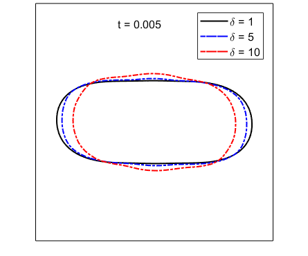
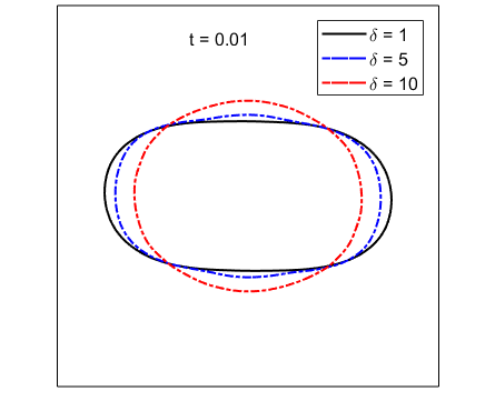
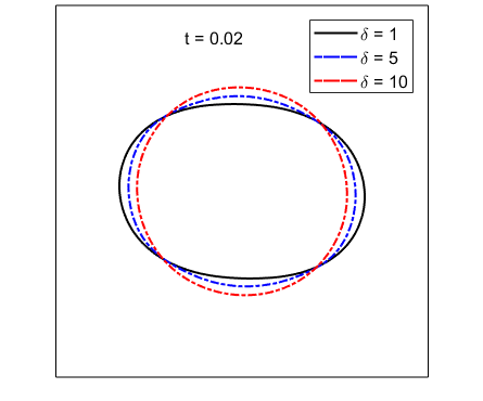
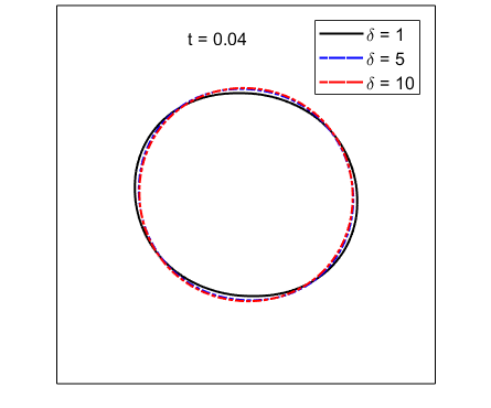
Figure 1: Test 2: Snapshots of the zero-level set of $\bar{u}_{h}$ at several time points with $\delta=1,5,10$ and $\epsilon=0.01$.

Next, we fix $\delta=1$ and study the influence of the parameter $\epsilon$ on the evolution of the numerical interfaces. In Figure 2, snapshots at four fixed time points of the zero-level set of $\bar{u}_{h}$ are depicted for three different $\epsilon=0.01,0.015,0.04$. Numerical results suggest the convergence of the numerical interface to the stochastic Hele-Shaw flow as $\epsilon\to 0$ at each of four time points. In addition, the numerical interface evolves faster in time for larger $\epsilon$.

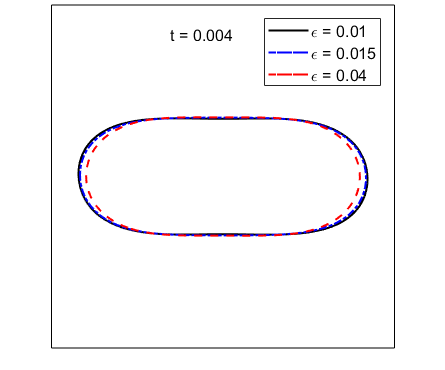
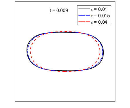
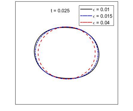
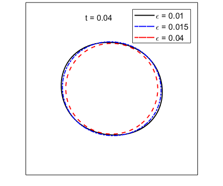
Figure 2: Test 2: Snapshots of the zero-level set of $\bar{u}_{h}$ at several time points with $\epsilon=0.01,0.015,0.04$ and $\delta=1$.

Notice that in Figure 1–2, we only plot the evolutions on the subdomain $[-0.6,0.6]^{2}$ for a better resolution.

In Figure 3, we plot the change of the expected value of the discrete energy

$$\mathbb{E}\left[{J(u^{n}_{h})}\right]\approx\frac{1}{M}\sum_{i=1}^{m}J(u^{n}_{h}(\omega_{i}))$$

in time with fixed $\epsilon=0.01$. It indicates that the decay property still holds for $\delta=1,5,10$.

Figure 3: Test 2: Decay of the expectation of numerical energy with $\epsilon=0.01$.

5.3 Test 3

In this test, we consider the case with

$$u_{0}(x)=\tanh\left(\frac{d_{0}(x)}{\sqrt{2}\epsilon}\right),$$

where $d_{0}(x)=\min\{d_{1}(x),d_{2}(x)\}$, and $d_{1}(x)$ and $d_{2}(x)$ denotes respectively the signed distance function to the ellipses

$$\frac{(x_{1}+0.2)^{2}}{0.15^{2}}+\frac{x_{2}^{2}}{0.45^{2}}=1\quad\text{and}\quad\frac{(x_{1}-0.2)^{2}}{0.15^{2}}+\frac{x_{2}^{2}}{0.45^{2}}=1.$$

In Figure 4, we depict snapshots at several time points of the zero-level set of $\bar{u}_{h}$ for $\delta=1,5,10$ with fixed parameter $\epsilon=0.01$. For all cases, the two separated zero-level sets eventually merge and evolve to a circular shape. For larger noise intensity ($\delta=5,10$), the two interfaces merge faster and develop two concentric interfaces where the outer interface evolves to a circular shape and the inner interface shrinks and eventually vanishes.

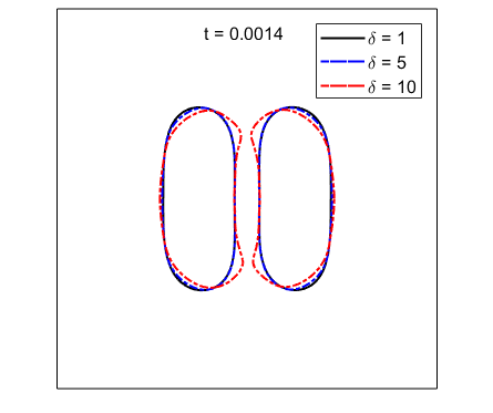
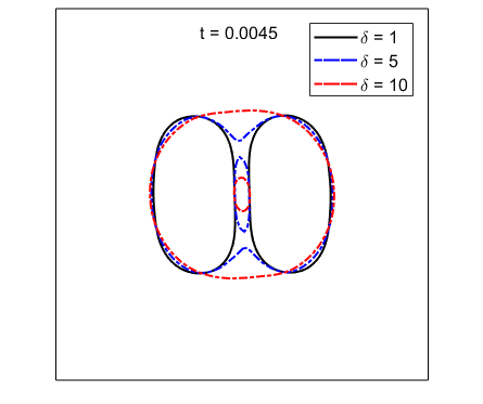
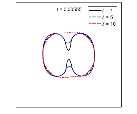
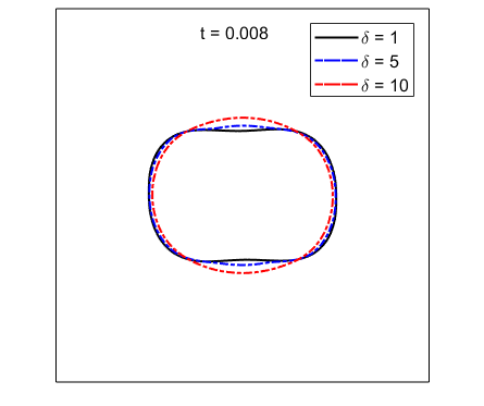
Figure 4: Test 3: Snapshots of the zero-level set of $\bar{u}_{h}$ at several time points with $\delta=1,5,10$ and $\epsilon=0.01$.

Next, we plot a few snapshots of the zero-level set of $\bar{u}_{h}$ for $\epsilon=0.01,0.015,0.04$ with fixed $\delta=1$ in Figure 5. Again, the numerical interface evolves faster in time for larger $\epsilon$, and the numerical interfaces stay close for $\epsilon=0.01$ and $\epsilon=0.015$.

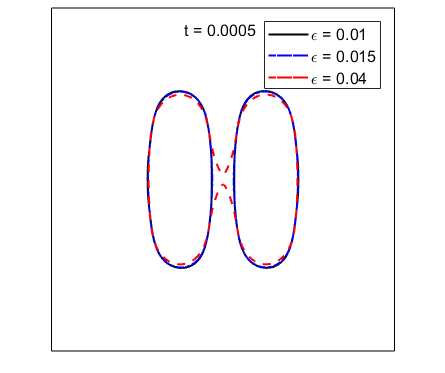
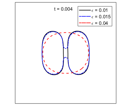
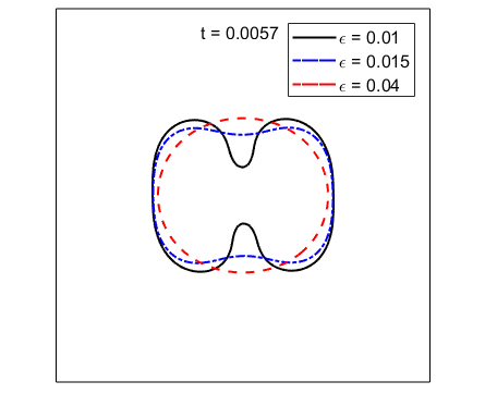
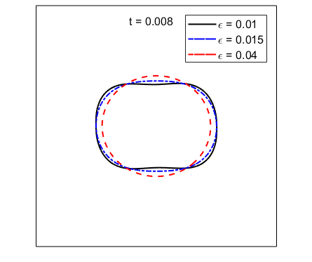
Figure 5: Test 3: Snapshots of the zero-level set of $\bar{u}_{h}$ at several time points with $\epsilon=0.01,0.015,0.04$ and $\delta=1$.

The decay of the expected value of the discrete energy is shown in Figure 6, where we consider three noise intensity levels $\delta=1,5,10$ with fixed $\epsilon=0.01$.

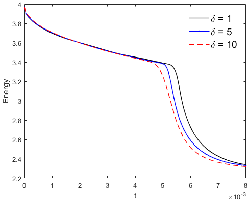
Figure 6: Test 3: Decay of the expectation of numerical energy with $\epsilon=0.01$.

References

[1] R. A. Adams, Sobolev Spaces, Academic Press, New York, 2003.
[2] N. D. Alikakos, P. W. Bates, and X. Chen, Convergence of the Cahn-Hilliard equation to the Hele-Shaw model, Arch. Rational Mech. Anal., 128(2), 165–205, 1994.
[3] A. C. Aristotelous, O. A. Karakashian and S. M. Wise,A mixed discontinuous
Galerkin, convex splitting scheme for a modified Cahn-Hilliard equation, Disc. Cont. Dynamic. Syst. Series B.,
18(9), 2211–2238, 2013.
[4]
D. M. Anderson, G. B. McFadden, and A. A. Wheeler, Diffuse-interface methods in fluid mechanics,
in Annual review of fluid mechanics, Vol. 30 of Annu. Rev. Fluid Mech., pages 139–165.
Annual Reviews, Palo Alto, CA, 1998.
[5] D. Blömker, S. Maiker-Paape, and T. Wanner, Spinodal decomposition for the stochastic Cahn-Hilliard equation, Trans. Amer. Math. Soc., 360, 449–489, 2008.
[6] S. C. Brenner and L. R. Scott, The Mathematical Theory of Finite Element Methods
(Third Edition), Springer-Verlag, New York, 2008.
[7] J. W. Cahn and J. E. Hilliard, Free energy of a nonuniform system I, Interfacial free energy, J. Chem. Phys., 28, 258–267, 1958.
[8] X. Chen, Global asymptotic limit of solutions of the Cahn-Hilliard equation,
J. Diff. Geom., 44(2), 262–311, 1996.
[9] P. Ciarlet, The Finite Element Method for Elliptic Problems. North-Holland, Amsterdam,
1978.
[10] H. E. Cook, Brownian motion in spinodal decomposition, Acta Metallurgica, 18, 297–306, 1970.
[11] Q. Du and X. Feng, The phase field method for geometric moving interfaces and
their numerical approximations, arXiv:1902.04924 [math.NA], 2019.
[12] D. Eyre. Unconditionally gradient stable time marching the
Cahn-Hilliard equation, In J.W. Bullard, R. Kalia, M. Stoneham, and L.Q. Chen, editors,
Computational and Mathematical Models of Microstructural Evolution, volume 53, pages
1686–1712, Warrendale, PA, USA, 1998. Materials Research Society.
[13] X. Feng, Y. Li and Y. Xing, Analysis of mixed interior penalty discontinuous
Galerkin methods for the Cahn–Hilliard equation and the Hele–Shaw flow, SIAM Journal on Numerical Analysis, 54(2), 825–847, 2016.
[14] X. Feng and A. Prohl, Error analysis of a mixed finite element method for the Cahn-Hilliard equation, Numer. Math., 74, 47–84, 2004.
[15] X. Feng and A. Prohl, Numerical analysis of the Cahn-Hilliard equation and approximation for the Hele-Shaw problem, Inter. and Free Bound., 7, 1–28, 2005.
[16] X. Feng, Y. Li and Y. Zhang, Strong convergence of a fully discrete finite element method for a class of semilinear stochastic partial differential equations with multiplicative noise, arXiv:1811.05028 [math.NA], 2018.
[17] X. Feng, Y. Li and Y. Zhang, Finite element methods for the stochastic
Allen-Cahn equation with gradient-type multiplicative noise, SIAM J. Numer. Anal., 55:194–216, 2017.
[18] T. Funaki, The scaling limit for a stochastic PDE and the separation of phases,
Probab. Theory Relat. Fields, 102, 221–288, 1995.
[19] D. Furihata, M. Kovács, S. Larsson, and F. Lindgren, Strong convergence of a fully discrete finite element approximation of the stochastic Cahn-Hilliard equation, SIAM J. Numer. Anal., 56, 708–731, 2018.
[20] V. Girault and P. Raviart, Finite Element Methods for Navier-Stokes Equations: Theory and Algorithms, vol. 5 of Springer Series in Computational Mathematics, Springer-Verlag, Berlin, 1986.
[21] M. Katsoulakis, G. Kossioris and O. Lakkis, Noise regularization and computations
for the -dimensional stochastic Allen-Cahn problem, Interfaces Free Bound., 9, 1–30, 2007.
[22] K. Kawasaki and T. Ohta, Kinetic drumhead model of interface. I, Progr.
Theoret. Phys., 67, 147–163, 1982.
[23] M. Kovács, S. Larsson, and F. Lindgren, On the backward Euler approximation of the stochastic Allen-Cahn equation, J. Appl. Probab., 52, 323–338, 2015.
[24] M. Kovács, S. Larsson, and F. Lindgren, On the discretisation in time of the stochastic Allen-Cahn equation, Math. Nachr., 291, 966-995, 2018.
[25] M. Kovács, S. Larsson, and A. Mesforush, Finite element approximation of the Cahn-Hilliard-Cook equation, SIAM J. Numer. Anal., 49, 2407–2429, 2011.
[26] M. Kovács, S. Larsson, and A. Mesforush, Erratum: Finite element approximation of the Cahn-Hilliard-Cook equation, SIAM J. Numer. Anal., 52, 2594–2597, 2014.
[27] N. V. Krylov and B. L. Rozovskii, Stochastic evolution equations,
In Stochastic Differential Equations: Theory and Applications: Interdisciplinary Math and Science,
World Science Publication, Hackensack, vol. 2, pp. 1–69, 2007.
[28] S. Larsson and A. Mesforush, Finite-element approximation of the linearized Cahn-Hilliard-Cook equation, IMA J. Numer. Anal., 31, 1315–1333, 2011.
[29] Y. Li, Error analysis of a fully discrete Morley finite element approximation for the Cahn-Hilliard equation, J. Sci. Comput. (to appear), 2019.
[30] Z. Liu and Z. Qiao, Wong–Zakai approximations of stochastic Allen-Cahn equation,
arXiv:1710.0953 [math.NA], 2017.
[31] G. Lord, C. Powell and T. Shardlow, An Introduction to Computational Stochastic
PDEs, Cambridge Texts in Applied Mathematics, CUP, 2014.
[32] A. K. Majee and A. Prohl, Optimal strong rates of convergence for a space-time discretization
of the stochastic Allen-Cahn equation with multiplicative noise, Comput. Methods Appl. Math., 18, 297–311, 2018.
[33] R. H. Nochetto and C. Verdi, Convergence past singularities for a
fully discrete approximation of curvature-driven interfaces, SIAM J. Numer. Anal., 34(2), 490–512, 1997.
[34] G. Da Prato and A. Debussche, Stochastic Cahn-Hilliard equation, Nonlinear Anal., 26, 241–263, 1996.
[35] G. Da Prato and J. Zabczyk, Stochastic Equations in Infinite Dimensions,
Cambridge University Press, 1992.
[36] C. Prévôt and M. Röckner, A Concise Course on Stochastic Partial
Differential Equations, Springer, 140, 2007.
[37] R. L. Pego, Front migration in the nonlinear Cahn-Hilliard equation, Proc. Roy. Soc. London Ser. A 422, 261–278, 1989.
[38] B. Rivière, Discontinuous Galerkin Methods for Solving Elliptic and Parabolic Equations: Theory and Implementation, Frontiers in Applied Mathematics, SIAM, 2008.
[39] M. Röger and H. Weber, Tightness for a stochastic Allen-Cahn equation, Stoch. PDE: Anal. Comp., 1, 175–203, 2013.
[40] B. Stoth, Convergence of the Cahn-Hilliard equation to the Mullins-Sekerka
problem in spherical symmetry, J. Diff. Eqs. 125, 154–183, 1996.
[41] S. Wu and Y. Li, Analysis of the Morley element for the Cahn-Hilliard equation and the Hele-Shaw flow, arXiv:1808.08581 [math.NA], 2018.
[42] N. K. Yip, Stochastic curvature driven flows, Lecture notes in pure and applied mathematics, 443–46, 2002.