Radiation in equilibrium with plasma and plasma effects on cosmic microwave background

Abstract

The spectrum of the radiation of a body in equilibrium is given by Planck’s law. In plasma, however, waves below the plasma frequency cannot propagate; consequently, the equilibrium radiation inside plasma is necessarily different from the Planck spectrum. We derive, using three different approaches, the spectrum for the equilibrium radiation inside plasma. We show that, while plasma effects cannot be realistically detected with technology available in the near future, there are a number of quantifiable ways in which plasma affects cosmic microwave background (CMB) radiation.

I Introduction

A system in thermodynamic equilibrium is often said to have a blackbody radiation spectrum given by Planck’s law. However, the Planck spectrum should be modified within a medium. Indeed, in plasma, for example, radiation below the plasma frequency $\omega_{p}$ cannot propagate. Thus, the equilibrium radiation inside plasma is necessarily different from the Planck spectrum. This paper is dedicated to the investigation of the equilibrium radiation inside plasma and to the study of the plasma effects and the possibility of their detection with respect to one of the most known examples of equilibrium radiation in nature – the cosmic microwave background (CMB).

In Sec. II we derive the equilibrium spectral energy density of radiation inside plasma using three different approaches: from the point of view of photons in plasma treating them as quasiparticles obeying Bose-Einstein statistics, from the point of view of plasma that generates electromagnetic fluctuations, and from the point of view of equilibrium between plasma and external blackbody radiation.

In Sec. III we consider several questions related to experimental measurements for stationary and moving observers inside a plasma universe. We distinguish quantities expressed in terms of frequency from quantities expressed in terms of wavelength. In a medium with unknown dispersion we also distinguish energy density from radiation intensity. We also calculate the Lorentz transformation for a moving observer inside plasma.

In Sec. IV we study plasma effects on CMB radiation. We consider the possibility of experimental detection of static and dynamical plasma effects on CMB but conclude that these effects cannot be detected in the next-generation experiments. We show that the static equilibrium distribution should have been significantly modified during the epoch of recombination and that this can manifest itself as an extremely small frequency-dependent chemical potential. We demonstrate that plasma changes the cosmological redshift and calculate how it distorts the equilibrium spectrum as the universe expands.

In Sec. V we consider how plasma modifies the Kompaneets equation both because of the change in the dispersion relation and because of coherent scattering in plasma.

In Sec. VI we consider plasma effects on CMB during and after the epoch of reionization. We calculate plasma corrections to Compton $y$-distortion due to the thermal Sunyaev–Zel’dovich effect. We identify a novel mechanism of magnetic field generation at the epoch of reionization resulting from conversion of some of the energy of CMB into the magnetic field.

We estimate the corrections that plasma effects can bring to other expected CMB distortions for Planck’s telescope (Tauber et al., 2010) and SKA-LOW (Dewdney et al., 2013) and conclude that plasma effects are extremely small, on the order of magnitude of $O\left(\omega_{p}^{2}/\omega^{2}\right)$ in most cases, and thus cannot be realistically detected in the near future.

II Radiation in thermodynamic equilibrium with plasma

Planck’s radiation spectrum is characterized only by one parameter – temperature, and it is nonzero for all frequencies. In equilibrium plasma, however, radiation with frequencies below the plasma frequency $\omega_{p}$ cannot propagate. Thus, the spectral energy density of radiation inside plasma is necessarily different from radiation in free space. Let us derive this spectrum using three different approaches.

II.1 Photons as quasiparticles

Photons are bosons and so they follow Bose-Einstein statistics that says that the average number of particles with given energy $\varepsilon$ is proportional to $\left[e^{\left(\varepsilon-\mu\right)/T}-1\right]^{-1}$. Thus, we can write the photon number $n_{\gamma}$ and energy densities $u_{\gamma}$ as

$$n_{\gamma}=\frac{1}{V}\sum_{\mathbf{k}}\frac{g_{\gamma}}{e^{\frac{\hbar\omega\left(\mathbf{k}\right)-\mu}{T}}-1},$$ (1)

$$u_{\gamma}=\frac{1}{V}\sum_{\mathbf{k}}\frac{g_{\gamma}\hbar\omega\left(\mathbf{k}\right)}{e^{\frac{\hbar\omega\left(\mathbf{k}\right)-\mu}{T}}-1}.$$ (2)

Planck’s law follows from these equations if the following assumptions are employed: $g_{\gamma}=2$, corresponding to two polarizations of electromagnetic waves; $\mu=0$, corresponding to zero chemical potential of photons that can be freely absorbed and emitted; non-dispersive light in vacuum with $\omega=kc$; and substitution of summation with integration $\left(1/V\right)\sum_{\mathbf{k}}\rightarrow\int d^{3}\mathbf{k}/\left(2\pi\right)^{3}$. Then Eq. (2) yields:

$$u_{Planck}=\frac{\hbar}{\pi^{2}c^{3}}\int_{0}^{\infty}\frac{\omega^{3}}{e^{\frac{\hbar\omega}{T}}-1}d\omega.$$ (3)

Throughout the paper we will use $u_{\omega}=du/d\omega$ for energy density per $d\omega$, which for blackbody Planck’s radiation we will denote as $u_{bb}$. We will also use $I_{\omega}$ for intensity per $d\omega$ defined as $I_{\omega}=v_{gr}u_{\omega}$, where $v_{gr}=\partial\omega/\partial k$ is the group velocity, and $I_{bb}$ for intensity per $d\omega$ for blackbody radiation.

Equation (2) shows that the radiation in thermodynamic equilibrium with plasma or any other matter can be different from Planck’s law for three reasons. First, because of dispersion of waves in matter, only certain waves with certain frequencies $\omega=\omega\left(\mathbf{k}\right)$ and, as a consequence, energy $\varepsilon\left(\mathbf{k}\right)=\hbar\omega\left(\mathbf{k}\right)$ can propagate in the medium for a given $\mathbf{k}$. Second, there is nonzero chemical potential $\mu\neq 0$. Though it is often approximated that light has zero chemical potential (for example, Refs. (Huang, 1987; Greiner et al., 1995)), it is not the case in general (Wurfel, 1982; Herrmann and Würfel, 2005). Chemical potential is related to constraints on the number of particles and such situations can be realized, for example, in semiconductors (Wurfel, 1982; Herrmann and Würfel, 2005; Ries and McEvoy, 1991; Markvart, 2008), where the number of photons is related to the number of electrons and holes; in plasmas when scattering dominates over absorption and thus the number of photons conserved (Zel’dovich and Levich, 1969); in dye filled microcavities (Klaers et al., 2010; Klaers, 2014); and in other systems (Hafezi et al., 2015; Wang et al., 2018; Meyer and Markvart, 2009). Third, there are geometrical and finiteness effects restricting the number of available $\mathbf{k}$ modes. The sum over $\mathbf{k}$ in $\sum_{\mathbf{k}}$ in general should be performed only over certain $\mathbf{k}$’s. For example, in cavities depending on the size and geometry only certain waves with given $\mathbf{k}$’s can exist (Reiser and Schächter, 2013; Sokolsky and Gorlach, 2014; McGregor, 1978).

Now let us consider the case of infinite plasma. The typical nonrelativistic plasma has the following dispersion relation for electromagnetic waves:

$$\omega^{2}=\omega_{p}^{2}+k^{2}c^{2},$$ (4)

where the plasma frequency is defined through the sum over the species of charged particles in plasma: $\omega_{p}^{2}=\sum_{s}4\pi n_{s}e_{s}^{2}/m_{s}$. Since photon energy is $\varepsilon=\hbar\omega$, we can rewrite Eq. (4) as

$$\varepsilon^{2}=m_{\gamma}^{2}c^{4}+p_{\gamma}^{2}c^{2},$$ (5)

i.e., in plasma, a photon behaves as a relativistic massive particle with mass $m_{\gamma}=\hbar\omega_{p}/c^{2}$ and momentum $p_{\gamma}=\hbar k$. It is interesting to calculate the density of electrons for which the effective photon mass equals the electron rest mass. It happens for electron density $n_{e}\approx(r_{e}\lambda_{C}^{2})^{-3}\approx 10^{31}\>\textrm{{c$\textrm{m}^{\textrm{-3}}$}}$ (corresponding plasma frequency is about $10^{20}\>\textrm{$\textrm{s}^{-1}$}$), where $r_{e}$ is the classical electron radius and $\lambda_{C}$ is the Compton wavelength. Thus, for extremely high density plasmas, photons can be expected to behave similarly to massive elementary particles like electrons.

Going from summation to integration and introducing dimensionless parameters $a=\hbar\omega_{p}/T$ and $\mu^{\prime}=\mu/T$, we can write the photon number and energy densities in terms of the normalized wave vector $y=\hbar kc/T$ as:

$$n_{\gamma}=\frac{T^{3}}{\pi^{2}\hbar^{3}c^{3}}\int_{0}^{\infty}\frac{y^{2}}{e^{\sqrt{y^{2}+a^{2}}-\mu^{\prime}}-1}dy,$$ (6)

$$u_{\gamma}=\frac{T^{4}}{\pi^{2}\hbar^{3}c^{3}}\int_{0}^{\infty}\frac{\sqrt{y^{2}+a^{2}}y^{2}}{e^{\sqrt{y^{2}+a^{2}}-\mu^{\prime}}-1}dy,$$ (7)

and in terms of the normalized frequency $x=\hbar\omega/T$ as:

$$n_{\gamma}=\frac{T^{3}}{\pi^{2}\hbar^{3}c^{3}}\int_{a}^{\infty}\frac{x^{2}}{e^{x-\mu^{\prime}}-1}dx,$$ (8)

$$u_{\gamma}=\frac{T^{4}}{\pi^{2}\hbar^{3}c^{3}}\int_{a}^{\infty}\frac{x^{2}\sqrt{x^{2}-a^{2}}}{e^{x-\mu^{\prime}}-1}dx.$$ (9)

Thus, the radiation distribution inside plasma is described by three parameters: temperature $T$, chemical potential $\mu$, and parameter $a=\hbar\omega_{p}/T$. The parameter $a$ is a measure of the density.

Using the expansion

$$\frac{1}{e^{\sqrt{y^{2}+a^{2}}-\mu^{\prime}}-1}=\sum_{l=1}^{\infty}e^{-l\left(\sqrt{y^{2}+a^{2}}-\mu^{\prime}\right)},$$ (10)

substituting $y=a\sinh\theta$, and employing the integral representation for the modified Bessel functions of the second kind, we can get the total number and energy densities:

$$n_{\gamma}=\frac{T^{3}}{\pi^{2}\hbar^{3}c^{3}}\sum_{l=1}^{\infty}\frac{e^{l\mu^{\prime}}}{l^{3}}\left(la\right)^{2}K_{2}\left(la\right),$$ (11)

$$u_{\gamma}=\frac{T^{4}}{\pi^{2}\hbar^{3}c^{3}}\sum_{l=1}^{\infty}\frac{e^{l\mu^{\prime}}}{l^{4}}\left[\left(la\right)^{3}K_{1}\left(la\right)+3\left(la\right)^{2}K_{2}\left(la\right)\right].$$ (12)

Similar expressions were obtained in Refs. (Bannur, 2006; Trigger, 2007; Triger and Khomkin, 2010; Medvedev, 1999; Tsintsadze et al., 1996; Mati, 2019).

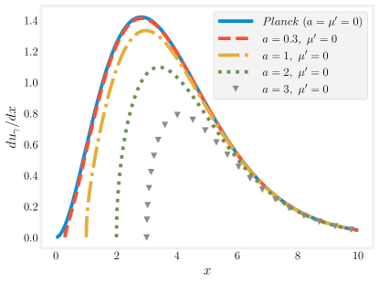
FIG. 1: Photon energy density in the units of $T^{4}/\pi^{2}\hbar^{3}c^{3}$ versus normalized frequency $x=\hbar\omega/T$ for different values of parameter $a$ and $\mu^{\prime}=0$ . Blackbody Planck density corresponding to $a=\mu^{\prime}=0$ is also shown for comparison.

Figure 1 shows spectral energy density $du_{\gamma}/dx$ in the units of $T^{4}/\pi^{2}\hbar^{3}c^{3}$ as a function of normalized frequency $x=\hbar\omega/T$ for several values of parameter $a=\hbar\omega_{p}/T$ and zero chemical potential. We see the truncation of the spectrum for frequencies below the plasma frequency as well as an overall decrease of the radiation density with growth of $a$. We also see that for $a\gtrsim 1$ the radiation density starts to significantly deviate from the Planck distribution, which corresponds to $a=\mu^{\prime}=0$.

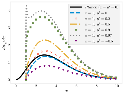
FIG. 2: Photon energy density in the units of $T^{4}/\pi^{2}\hbar^{3}c^{3}$ versus normalized frequency $x=\hbar\omega/T$ for different values of chemical potential $\mu^{\prime}$ and $a=1$. Blackbody Planck density corresponding to $a=\mu^{\prime}=0$ is also shown for comparison.

Figure 2 shows spectral energy density $du_{\gamma}/dx$ in the units of $T^{4}/\pi^{2}\hbar^{3}c^{3}$ as a function of normalized frequency $x=\hbar\omega/T$ for fixed parameter $a=1$, but different chemical potentials. Despite the occasional claim that bosons can have only zero or negative chemical potential (for example, Refs. (Greiner et al., 1995; Chen and Lin, 2003)), in fact they can have positive chemical potential too; the only restriction is that the smallest energy level is larger than zero and the corresponding integrals converge. We see that the chemical potential can affect the distribution significantly. However, we do not address the question of whether a particular chemical potential can be realistically achieved in any physical system. Note also that Fig. 2 does not correspond to one system with given $a$ and different chemical potentials, but to several independent systems with different number of photons. For a given system with a fixed number of photons, one cannot vary the chemical potential independent of $T$ and $a$; see Ref. (Mati, 2019) for details.

Figure 2 also suggests that the radiation energy can exceed Planck’s radiation density. However, it does not contradict the often-made statement that thermal blackbody radiation establishes the upper limit on the maximum energy emitted for any body at the same temperature (for example, Refs. (Bohren and Huffman, 1983; Massoud, 2005)), because Fig. 2 shows the energy density inside the plasma and not the intensity that will be emitted by plasma. Moreover, objects for which the absorption cross section exceeds the geometrical cross section can actually emit more than blackbody, but this does not contradict standard physics and fits the generalized form of Kirchhoff’s law (Greffet et al., 2018).

II.2 Fluctuation-dissipation theorem

So far we have derived properties of equilibrium radiation from the point of view of photons obeying Bose-Einstein statistics. Since the radiation is in equilibrium with the matter, the same results should be obtained by considering oscillating electrons in plasma and calculating the density of the electromagnetic field generated by them using the fluctuation-dissipation theorem (Triger and Khomkin, 2010; Lifshitz and Pitaevskii, 1980).

Following Ref. (Lifshitz and Pitaevskii, 1980), the spectral energy density per $d\omega$ in a transparent medium with dielectric function $\varepsilon\left(\omega\right)$ is given by

$$u_{\gamma}=\int_{0}^{\infty}\frac{1}{8\pi}\left[2\left(E^{2}\right)_{\omega}\frac{\partial\left(\omega\varepsilon\right)}{\partial\omega}+2\left(H^{2}\right)_{\omega}\right]\frac{d\omega}{2\pi},$$ (13)

where the fluctuations $\left(E^{2}\right)_{\omega}$ and $\left(H^{2}\right)_{\omega}$ of the electric and magnetic fields are defined through

$$\left\langle\mathbf{E}^{2}\right\rangle=\int_{-\infty}^{\infty}\left(E^{2}\right)_{\omega}\frac{d\omega}{2\pi}=\int_{0}^{\infty}2\left(E^{2}\right)_{\omega}\frac{d\omega}{2\pi},$$ (14)

$$\left\langle\mathbf{H}^{2}\right\rangle=\int_{-\infty}^{\infty}\left(H^{2}\right)_{\omega}\frac{d\omega}{2\pi}=\int_{0}^{\infty}2\left(H^{2}\right)_{\omega}\frac{d\omega}{2\pi}.$$ (15)

According to Ref. (Lifshitz and Pitaevskii, 1980), the electromagnetic field fluctuations can be expressed as

$$\left(E^{2}\right)_{\omega}=\frac{1}{\varepsilon}\left(H^{2}\right)_{\omega}=\frac{2\omega^{2}\hbar\varepsilon^{\frac{1}{2}}}{c^{3}}\coth\frac{\hbar\omega}{2T}\\ =\frac{4\omega^{2}\hbar\varepsilon^{\frac{1}{2}}}{c^{3}}\left(\frac{1}{2}+\frac{1}{e^{\frac{\hbar\omega}{T}}-1}\right),$$ (16)

so we have

$$du_{\gamma}=\frac{\hbar\omega^{2}\varepsilon^{\frac{1}{2}}}{2\pi^{2}c^{3}}\left[\frac{\partial\left(\omega\varepsilon\right)}{\partial\omega}+\varepsilon\right]\left(\frac{1}{2}+\frac{1}{e^{\frac{\hbar\omega}{T}}-1}\right)d\omega.$$ (17)

Using $\varepsilon\left(\omega\right)=1-\omega_{p}^{2}/\omega^{2}$ for plasma and ignoring zero-field fluctuations ($1/2$ term), we get the same result for the spectral energy density of radiation in plasma as previously obtained: Eq. (9) with $\mu=0$ .

II.3 Equilibrium with blackbody walls

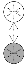
FIG. 3: Equilibrium between blackbody radiation and plasma, showing detailed balance among emission, absorption, and reflection.

Consider a lossless medium (plasma) surrounded by blackbody walls at temperature $T$ and being in equilibrium with them (see Fig. 3). Let us look at a ray of frequency $\omega_{0}$ and energy $u_{bb}\left(\omega_{0}\right)d\omega_{0}$, which is emitted by the blackbody walls, and then propagates through vacuum and impinges on the medium at angle $\theta_{0}$ to its normal. The wave will experience refraction, such that its frequency remains the same ($\omega=\omega_{0}$), while its wave vector changes. A change in the wave vector implies a change in aperture. Specifically, using Snell’s law $n=c/v_{ph}=\sin\theta_{0}/\sin\theta$, the solid angle $d\Omega=2\pi\sin\theta d\theta$ in plasma can be expressed through the original solid angle as:

$$d\Omega=\left(\frac{v_{ph}}{c}\right)^{2}\frac{\cos\theta_{0}}{\cos\theta}d\Omega_{0},$$ (18)

which is the well-known étendue conservation condition (Markvart, 2008).

In addition, the group velocity, which determines the energy transport, changes in the medium. Since in lossless medium the energy must be conserved, the pulse must be shortened or stretched depending, correspondingly, on whether the group velocity in the medium is smaller or larger than in vacuum.

Finally, only part of the energy of the wave will be transmitted into the medium, because part of the wave will be reflected. The reflection coefficient for unpolarized light is $R=\left(R_{s}+R_{p}\right)/2$, where $R_{s}$ and $R_{p}$ are the reflectances of $s$-polarized and $p$-polarized electromagnetic waves given by the Fresnel equations. The transmission coefficient is given by $1-R$.

Taking into account both the change in the aperture and the group velocity, we can write the energy conservation law:

$$\left(1-R\right)u_{bb}c\cos\theta_{0}d\omega_{0}d\Omega_{0}+Ru_{\omega}v_{gr}\cos\theta d\omega d\Omega\\ =u_{\omega}v_{gr}\cos\theta d\omega d\Omega.$$ (19)

Here the first term on the left-hand side is the transmitted energy, while the second term is the energy of the wave incident on the medium-vacuum interface at angle $\theta$ from within the medium and reflected back. Notice that the reflection coefficients coincide because the reflectance of the light incident from medium 1 on medium 2 at the angle $\theta_{i}$ and refracted into the angle $\theta_{t}$ is the same as the reflectance of the light incident from medium 2 on medium 1 at the angle $\theta_{t}$. Thus, using Eqs. (18) and (19), we get that the energy density inside the medium is independent of the reflection coefficient $R$ and is given by

$$u_{\omega}=\frac{c^{3}}{v_{gr}v_{ph}^{2}}u_{bb}.$$ (20)

For plasma $v_{gr}=\partial\omega/\partial k=c\sqrt{1-\omega_{p}^{2}/\omega^{2}}$ , $v_{ph}=\omega/k=c/\sqrt{1-\omega_{p}^{2}/\omega^{2}}$, and using the Planck energy density, we again get the same result for the electromagnetic radiation energy density inside plasma as before.

The above result can also be considered through the radiation transfer equation in the medium (Bekefi, 1966; Zheleznyakov, 1996):

$$n_{r}^{2}\frac{d}{dl}\left(\frac{I_{\omega}}{n_{r}^{2}}\right) = \frac{1}{v_{gr}}\frac{\partial I_{\omega}}{\partial t}+n_{r}^{2}\frac{\partial}{\partial l}\left(\frac{I_{\omega}}{n_{r}^{2}}\right)=\alpha_{\omega}-\mu_{\omega}I_{\omega},$$ (21)

where $I_{\omega}$ is the ray intensity per $d\omega$ and is related to the energy density through group velocity as $u_{\omega}=du/d\omega=I_{\omega}/v_{gr}$, $n_{r}$ is the ray refractive index, which is the usual refractive index for isotropic medium (see Ref. (Bekefi, 1966)), $\alpha_{\omega}$ is emissivity, and $\mu_{\omega}$ is the absorption coefficient (including scattering).

The condition of transparency of the medium, which corresponds to $\alpha_{\omega}=\mu_{\omega}=0$ and makes the right-hand side of the radiation transfer equation zero, results in $I_{\omega}/n^{2}=const$ along the ray. The condition $I_{\omega}/n^{2}=const$ gives $I_{\omega}=n^{2}I_{bb}=\left(1-\omega_{p}^{2}/\omega^{2}\right)I_{bb}$, i.e., the same radiation energy density inside plasma as before. The condition $I_{\omega}/n^{2}=const$ also means that $I_{\omega}$ is constant inside plasma as expected for transparent medium. However, another way to make the right-hand side zero is to have $\alpha_{\omega}/\mu_{\omega}=I_{\omega}$. In this case $I_{\omega}$ is constant inside the medium as well; not because the medium does not absorb and emit radiation at all, but because it does so in a very particular way. This is what actually happens in plasma, where equilibrium is reached through balance between emission and absorption (and scattering).

We emphasize that $u_{\omega}$ is the energy density inside the bulk of the plasma and does not determine the radiation emitted from the plasma. The radiation leaving the plasma experiences refraction and lengthening in accordance with the above formulas such that emission from equilibrium plasma above the plasma frequency is just that of a blackbody given by the Stefan-Boltzmann law, as expected in equilibrium. Below the plasma frequency, plasma is a perfect reflector. There must also be plasma waves along the surface of the boundary. However, the boundary effects at the plasma-vacuum interface are a separate and intricate topic beyond the scope of the considerations here.

III Measuring plasma spectrum by stationary and moving observers

Let us consider the experimental detection of radiation inside plasma (or, in general, any kind of dispersive medium). Imagine we have two observers: one is in a plasma-filled universe in thermodynamic equilibrium at temperature $T$ and the other is immersed in blackbody radiation of the same temperature $T$ in vacuum. Imagine both have identical devices manufactured and calibrated in vacuum that allow them measure electromagnetic radiation spectrum. What would the observers actually measure and how should these results be interpreted? Will they be able to see the difference?

First, we should say that it is intensity and not energy density that is being measured. In vacuum they are related through the speed of light, but in the medium they are related through the group velocity, which depends on unknown properties of the medium. Second, in vacuum the wavelength and frequency are related through the speed of light ($\omega=2\pi c/\lambda$), so any physical quantity expressed in terms of frequency can be immediately expressed in terms of wavelength; for example, if we know intensity per frequency $I_{\omega}$, then we immediately know intensity per wavelength $I_{\lambda}$. In the medium frequency and wavelength are related through $\omega=2\pi c/\lambda n\left(\omega\right)$, i.e., the conversion depends on unknown properties of the medium. Thus, we should be specific whether the observer in plasma measures at the same wavelength or at the same frequency as in vacuum.

We can imagine that the observer with a measuring instrument is in a small vacuum bubble inside the plasma or the measuring instrument is in direct contact with plasma. In any case, since the light ray traveling through two different mediums keeps its frequency but changes its wavelength, all the observable quantities should be expressed in terms of frequency, i.e., the observer will measure intensity per frequency $I_{\omega}$. If the bubble is in equilibrium with plasma, then, from the analysis of the previous section, it is apparent that the radiation inside the bubble would be that of blackbody and the device in equilibrium with plasma universe would register just blackbody radiation spectrum. Thus, the bubble should not be in equilibrium and, ideally, the measuring instruments should not radiate. This can be achieved by keeping the temperature of the measuring instruments close to absolute zero as is done, for example, on Planck’s telescope where the active refrigeration system keeps the HFI detector temperature at $0.1\>\textrm{K}$ (Tauber et al., 2010). Another effect that should be taken into account when interpreting the experimental results is that the telescope has inevitable reflections. They can be accounted for in vacuum, but, in the plasma universe, the reflection coefficient will be different and generally speaking unknown. Thus, the observer will measure $\left[1-R\left(\omega\right)\right]I_{\omega}$, where the reflection coefficient $R\left(\omega\right)$ is not known.

Finally, we address how the spectrum changes for a moving observer. Since the Doppler shift depends on properties of the medium, the transformation of the spectrum in the moving reference frame would be different than that in vacuum. As shown in Ref. (Bičák and Hadrava, 1975) for the emitted and observed intensities, the following relationship holds true:

$$\frac{I_{\omega}}{\omega^{3}n^{2}}=const.$$ (22)

In vacuum, the frequency experiences Doppler shift $\omega=\gamma\left(\omega^{\prime}+\mathbf{k}^{\prime}\mathbf{v}\right)=\gamma\omega^{\prime}\left(1+\beta\cos\theta^{\prime}\right)$ and the blackbody radiation for a moving observer becomes

$$I_{\omega\prime}^{\prime}=\frac{\omega^{\prime 3}}{\omega^{3}}I_{\omega}=\frac{\omega^{\prime 3}}{\omega^{3}}I_{bb}=\frac{\hbar}{\pi^{2}c^{2}}\frac{\omega^{\prime 3}}{e^{\frac{\hbar\omega\prime}{T^{\prime}}}-1},$$ (23)

i.e., for the moving observer the radiation spectrum appears as blackbody but with new effective directional temperature $T^{\prime}=T/\gamma\left(1+\beta\cos\theta^{\prime}\right)$.

For a moving observer in the plasma universe:

$$I_{\omega\prime}^{\prime}=\frac{\omega^{\prime 3}n^{\prime 2}}{\omega^{3}n^{2}}I_{\omega}=\frac{\omega^{\prime 3}}{\omega^{3}}n^{\prime 2}I_{bb}=\frac{\hbar}{\pi^{2}c}\frac{\omega^{\prime 3}n^{\prime 2}}{e^{\frac{\hbar\omega}{T}}-1}.$$ (24)

Using the Lorentz transformation we can express $n^{\prime}$ and $\omega$ in terms of $\omega^{\prime}$ and $\theta^{\prime}$ to get the expression for $I_{\omega\prime}^{\prime}$ in the moving frame. We cannot find the analytical expression for a general medium, but, luckily, for plasma, the dispersion relation is Lorentz invariant:

$$\omega^{\prime 2}-k^{\prime 2}c^{2}=\omega^{2}-k^{2}c^{2}=\omega_{p}^{2},$$ (25)

so that the refractive index for a moving observer has the same functional dependance as for the stationary observer: $n^{\prime}=ck^{\prime}/\omega^{\prime}=1-\omega_{p}^{2}/\omega^{\prime 2}$. Thus, the intensity measured by the moving observer in plasma is

$$I_{\omega\prime}^{\prime}=\frac{\hbar}{\pi^{2}c}\frac{\omega^{\prime}\left(\omega^{\prime 2}-\omega_{p}^{2}\right)}{e^{\frac{\hbar\omega^{\prime}}{T^{\prime}}}-1},$$ (26)

i.e., for the moving observer the radiation spectrum appears as that of equilibrium radiation in plasma but with new frequency-dependent effective directional temperature $T^{\prime}=T/\gamma\left(1+\beta\sqrt{1-\omega_{p}^{2}/\omega^{\prime 2}}\cos\theta^{\prime}\right)$.

In reality most of the plasmas are not in thermal equilibrium. If we are interested in radiation from the plasma, we should know specific emission mechanism in plasma and its optical depth. The most prominent example of the equilibrium radiation in nature is CMB. We are going to study plasma effects on it in the next section.

IV Early universe and plasma effects on CMB

According to accepted cosmology models, the radiation in the early universe and ionized matter (plasma) were tightly coupled and thermalized due to Thomson scattering, until, at cosmological redshift $z\approx 1100$, because of the recombination, the radiation became decoupled from now essentially neutral matter. This radiation from the early universe is known as CMB.

Experimental data show that CMB spectrum is consistent with Planck’s law to very high accuracy (Fixsen, 2009). In principle, however, since before the recombination the universe was in the plasma state for which waves with frequencies below the plasma frequency $\omega_{p}$ cannot propagate, the radiation inside it should have been different from the Planck spectrum. For this reason, in this section we discuss the influence of plasma effects on CMB and the possibility of the experimental observation of new effects.

IV.1 Direct detection of plasma spectrum

A comparison of the equilibrium radiation in plasma given by Eq. (9) with experimental data on CMB radiation was investigated in Ref. (Colafrancesco et al., 2015). Three methods of the detection of plasma dispersion effects were proposed. One is the direct observation of the plasma effects, specifically, the cutoff at plasma frequency, by comparing experimental data on CMB with the distribution given by Eq. (9). The second is the modification of the Sunyaev-Zel’dovich effect as the plasma modified CMB radiation travels through the electron gas of galaxy clusters. The third is the modification of the cosmological 21-cm background radiation. The conclusion reached in Ref. (Colafrancesco et al., 2015) can be summarized as that, even though the currently available experimental data cannot show any plasma effects, they might be detectable with the new generation of low-frequency experiments such as SKA-LOW. We argue that the conclusion reached in Ref. (Colafrancesco et al., 2015) is too optimistic for two reasons.

First, the values of parameter $a=(3.63,\>6.10,\>7.36)\times 10^{-3}$ used in Ref. (Colafrancesco et al., 2015) were estimated through a numerical fit to COBE-FIRAS data, to some other data in the range $\sim$$1.3\text{\textendash}50\>\textrm{GHz}$ (see Ref. (Colafrancesco et al., 2015)), and to three low-frequency data points from Refs. (Howell and Shakeshaft, 1967; Sironi et al., 1990, 1991). This procedure of obtaining $a$ is likely to significantly overestimate it, because the value of $a$ is mostly determined by the above mentioned three low-frequency data points, which, besides having high uncertainty, can give only the upper limit on $a$. Simply put, in this case the parameter $a$ is essentially approximated by the lowest experimental value available, but the absence of low-frequency data should not determine the plasma frequency, which actually can be much lower than the lowest experimental value. Indeed, the value of parameter $a$ estimated through the electron density ($n_{e}\approx 300\>\textrm{cm}^{-3}$ (Triger and Khomkin, 2010)) and the CMB temperature ($T/k_{B}\approx 3000\>\textrm{K}$) just before the recombination gives orders of magnitude lower value $a\approx 2\times 10^{-9}$. Plasma dispersion brings corrections on the order of $O\left(a^{2}/x^{2}\right)$ or $O\left(\omega_{p}^{2}/\omega^{2}\right)$, which is a small number. Indeed, the value of electron density just before the recombination is $n_{e}\approx 300\>\textrm{cm}^{-3}$ (Triger and Khomkin, 2010), with corresponding plasma frequency $\omega_{p}\approx 10^{6}\>\textrm{$\textrm{s}^{-1}$}$. The smallest frequency measurable by Planck’s spacecraft is $\nu_{min}=30\>\textrm{GHz}$ (Tauber et al., 2010), which corresponds to $\omega=2\pi\nu\left(1+z\right)\approx 2\times 10^{14}\>\textrm{$\textrm{s}^{-1}$}$ at $z\approx 1100$, giving $\omega_{p}^{2}/\omega^{2}\approx 2\times 10^{-17}$. For the proposed SKA-LOW experiment, the minimum frequency is $\nu_{min}=50\>\textrm{MHz}$ (Dewdney et al., 2013), which corresponds to $\omega=2\pi\nu\left(1+z\right)\approx 3\times 10^{11}\>\textrm{$\textrm{s}^{-1}$}$ at $z\approx 1100$, giving $\omega_{p}^{2}/\omega^{2}\approx 8\times 10^{-12}$.

Second, even if, before the recombination, the CMB spectrum were given by Eq. (9), it would have been modified significantly during the recombination. The after-recombination spectrum of CMB depends on how fast the recombination happened. If it were so slow that full thermal equilibrium was maintained at every step (this requires destruction and creation of photons), then, after the recombination, we would get the radiation spectrum (9) with the parameter $a$ equal to zero (for simplicity, we consider complete recombination into neutral state, in reality the electron density decreases by about a factor of $10^{3}-10^{4}$ (Sunyaev and Chluba, 2009)), which is just the Planck distribution (maybe with nonzero $\mu$) and no plasma dispersion effects would be present. If, on the other hand, the recombination were so sudden that the number of photons is conserved, then the wave vector (and wavelength) of each radiation mode would remain constant, while the frequency would change: $k=k_{0}$, $\omega=kc=\sqrt{\omega_{0}^{2}-\omega_{p}^{2}}$. The number of photons $dn_{\gamma}$ would not change, the total energy density of photons would decrease (part of the initial energy would be converted into heat), and the energy spectrum would become

$$u_{\gamma}=\frac{T^{4}}{\pi^{2}\hbar^{3}c^{3}}\int_{0}^{\infty}\frac{x^{3}}{e^{\sqrt{x^{2}+a^{2}}-\mu^{\prime}}-1}dx.$$ (27)

This is consistent with the adiabatic formula from Ref. (Dodin and Fisch, 2010a) that says that the energy density per frequency [$du_{\gamma}\left(x\right)/x$] remains constant as the density of plasma changes. Adiabatic here means slow in comparison with period of the wave $d\ln\omega_{p}/dt\ll\omega$ making the number of waves an adiabatic invariant, but not so slow that the full equilibrium is established. The amount of energy taken from CMB and converted to heat can be approximated for small values of $a$ as $\triangle u_{\gamma}/u_{\gamma}=5a^{2}/2\pi^{2}$. Notice, though, that part of this energy would be radiated back into CMB because excited recombined atoms would radiate photons as they fall back into the ground state. The detailed physics of this process is complicated; the thorough numerical calculations can be found in Ref. (Chluba and Ali-Haïmoud, 2016). According to standard cosmology, the active cosmological hydrogen recombination happened between $z\approx 1600$ and $z\approx 800$ and the electron density decreased from $1$ to about $10^{-4}-10^{-3}$ (Sunyaev and Chluba, 2009). Thus, the adiabatic scenario should have been realized.

Let us compare the spectral energy density given by Eq. (27) with the original spectral energy density in plasma given by Eq. (9). Figure 4 shows the spectral energy density versus the normalized frequency for $a=1.0$ before and after sudden recombination, as well as the blackbody spectrum for the same temperature. We see that the distribution after the sudden recombination resembles the blackbody spectrum with different temperature. Most importantly, it does not have cutoff at low frequencies. For small $a$, the difference between the spectral radiation after the sudden recombination and that of blackbody is especially hard to notice as demonstrated in Fig. 5 for $a=0.1$. We remind the reader that the estimate for parameter $a$ just before the recombination is $a\approx 2\times 10^{-9}\ll 1$. Since Eq. (27) with $\mu^{\prime}=0$ has $e^{\sqrt{x^{2}+a^{2}}}-1\approx e^{x+a^{2}/2x}-1$ in the denominator in contrast to $e^{x}-1$ for the blackbody spectrum, then, for $x\gg a$, plasma effects can appear as frequency-dependent chemical potential $\mu_{CMB}=a^{2}/2x$ (see definition of $\mu_{CMB}$ in the next subsection). However, this chemical potential is extremely small. Indeed, for $x=2.8$, which corresponds to the maximum of the blackbody spectrum, $\mu_{CMB}$ has a negligible value of about $7\times 10^{-19}$, for $x_{min}=5\times 10^{-1}$ corresponding to the smallest frequency measured by Planck’s spacecraft $\mu_{CMB}\approx 4\times 10^{-18}$, and for the SKA-LOW experiment $x_{min}=9\times 10^{-4}$ and $\mu_{CMB}\approx 2\times 10^{-15}$. For reference, $\mu$-distortion expected from different processes in $\Lambda$CDM cosmology is about $10^{-9}-10^{-8}$ (Chluba, 2016). This is itself a very small quantity and has not been experimentally detected yet, but still, it is about 6 to 10 orders of magnitude higher than the chemical potential from plasma effect described above.

The recombination was not complete but the electron density decreased in $10^{4}$ times, which gives parameter $a\approx 2\times 10^{-11}$ just after the recombination. It is obvious, though, that detection of the effects related to this, even smaller parameter $a$, is harder.

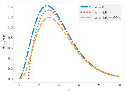
FIG. 4: Photon spectral energy density in the units of $T^{4}/\pi^{2}\hbar^{3}c^{3}$ versus normalized frequency $x=\hbar\omega/T$ for $a=1$, $\mu=0$ before and after sudden recombination, and for a blackbody of the same temperature with $a=0,\>\mu=0$.

FIG. 5: Photon spectral energy density in the units of $T^{4}/\pi^{2}\hbar^{3}c^{3}$ versus normalized frequency $x=\hbar\omega/T$ for $a=0.1$, $\mu=0$ before and after sudden recombination, and for a blackbody of the same temperature with $a=0,\>\mu=0$.

Thus, the detection of plasma dispersion effects on CMB, such as the existence of the lower-frequency cutoff, is much harder than suggested in Ref. (Colafrancesco et al., 2015). Even if the spectrum of CMB were indeed given by Eq. (9) before the recombination, after the recombination, the plasma dispersion effects could have been erased almost completely.

IV.2 Plasma modification of redshift

Another apparent plasma effect is change in redshift. The usual cosmological redshift is described by

$$\frac{\dot{\omega}}{\omega}=-\frac{\dot{a}_{sc}}{a_{sc}},$$ (28)

where $a_{sc}\left(t\right)=1/(1+z)$ is the cosmic scale factor and is not related to parameter $a=\hbar\omega_{p}/T$. In a dispersive medium Eq. (28) takes different form (Bičák and Hadrava, 1975):

$$\frac{\dot{\omega}}{\omega}=-\left(1+\frac{\omega}{n}\frac{\partial n}{\partial\omega}\right)^{-1}\left(\frac{\dot{a}_{sc}}{a_{sc}}+\frac{\dot{n}}{n}\right),$$ (29)

where the time derivative in $\dot{n}$ is not applied to $\omega$ in $n$. For plasma it gives a frequency-dependent redshift

$$\frac{\dot{\omega}}{\omega}=-\left(1+\frac{1}{2}\frac{\omega_{p}^{2}}{\omega^{2}}\right)\frac{\dot{a}_{sc}}{a_{sc}},$$ (30)

which is consistent with the expression obtained in Ref. (Dodin and Fisch, 2010b).

According to Eq. (28), frequency scales as $1+z$, and since temperature also scales as $1+z$, their ratio $x=\hbar\omega/T$ is scale invariant, so that the blackbody radiation spectrum remains blackbody-shaped as the universe expands. In contrast, according to Eq. (30), the frequency does not scale simply as $1+z$ anymore, suggesting that in plasma the shape of the spectrum does not remain the same as the universe expands. Intuitively, it is because light, which is inherently relativistic, in plasma acquires some properties of the matter, which is nonrelativistic. For ultrarelativistic plasma the plasma frequency is $\omega_{p}^{2}=4\pi ne^{2}c^{2}/3T$. In this case the frequency would grow in the same way as temperature.

It is believed that the universe was in full equilibrium at $z_{0}=2\times 10^{6}$, which defines the blackbody surface (Khatri and Sunyaev, 2012). In the absence of plasma and purely under the influence of cosmological redshift (no distortions) the blackbody spectrum at $z_{0}$ would be transformed into another blackbody spectrum at $z=1100$ with the new temperature $T=T_{0}\left(1+z\right)/\left(1+z_{0}\right)$. Now, with plasma, the full equilibrium spectrum at $z_{0}$ was given by Eq. (9) with zero chemical potential. From Eq. (30) we obtain $\left(\omega^{2}-\omega_{p}^{2}\right)/\left(\omega_{0}^{2}-\omega_{p0}^{2}\right)=\left(1+z\right)^{2}/\left(1+z_{0}\right)^{2}$ (Bičák and Hadrava, 1975) and, using $\omega_{p}^{2}\propto n_{e}\propto\left(1+z\right)^{3}$, we can calculate what the full equilibrium spectrum at $z_{0}=2\times 10^{6}$ would look like at $z=1100$ under plasma modified cosmological redshift (ignoring all other processes causing distortion):

$$du_{\gamma}=\frac{T^{4}}{\pi^{2}\hbar^{3}c^{3}}\frac{x\sqrt{x^{2}-a^{2}}\sqrt{x^{2}+\frac{z_{0}-z}{1+z}a^{2}}}{e^{\sqrt{x^{2}+\frac{z_{0}-z}{1+z}a^{2}}}-1}dx.$$ (31)

We see that while plasma redshift does not change the cutoff frequency it brings additional corrections on the order of $a^{2}\left(z_{0}-z\right)/\left(1+z\right)\approx a^{2}\left(z_{0}/z\right)\approx 4\times 10^{-15}$, i.e., these corrections are determined by parameter $a_{0}=a\left(1+z_{0}\right)^{1/2}/\left(1+z\right)^{1/2}\approx a\left(z_{0}/z\right)^{1/2}$ at $z_{0}=2\times 10^{6}$ rather than parameter $a$ at $z=1100$. In particular it can manifest itself as a frequency-dependent chemical potential $\mu_{CMB}\approx\left(z_{0}/z\right)a^{2}/2x$. This chemical potential is about $\left(z_{0}/z\right)\approx 10^{3}$ times larger than the one considered in the previous subsection but it is still beyond the values that can be experimentally detected. In addition, we note that for SKA-LOW at its lowest frequency $\nu_{min}=50\>\textrm{MHz}$, CMB foregrounds are going to further complicate measurements. Thus, the plasma correction to the redshift is extremely small and can hardly be detected by any past and near future CMB experiments.

Similar plasma redshift corrections would take place after the recombination for lower redshifts before (since the recombination is not complete) and after the reionization, but these corrections are smaller, since parameter $a$ at $z_{0}=2\times 10^{6}$ is higher.

V Modification of the Kompaneets equation

The standard way to describe the thermalization of the radiation and electrons through Thomson scattering and to quantify distortions of CMB from blackbody is to use the Kompaneets equation (Kompaneets, 1957) ($x_{e}=\hbar\omega/T_{e}$):

$$\frac{\partial n_{\gamma}}{\partial t}=\frac{n_{e}\sigma_{T}T_{e}}{m_{e}c}\frac{1}{x_{e}^{2}}\frac{\partial}{\partial x_{e}}\left[x_{e}^{4}\left(\frac{\partial n_{\gamma}}{\partial x_{e}}+n_{\gamma}+n_{\gamma}^{2}\right)\right],$$ (32)

where $\sigma_{T}$ is the Thomson cross section.

The equilibrium solution ($\partial n_{\gamma}/\partial t=0$) of this equation is given by the Bose-Einstein distribution with, in general, nonzero chemical potential $\mu$ (we note that it is customary to use a different sign convention for chemical potential in CMB science in comparison with the statistical mechanics literature: $\mu_{CMB}=-\mu^{\prime}=-\mu/T$). The chemical potential appears because Eq. (32) accounts only for scattering and, consequently, conserves the number of photons. This deviation from the Planck distribution is known as $\mu$-distortion. If it exists, $\mu$-distortion is very small: according to the COBE-FIRAS data the constraint on $\mu$ is $\left|\mu\right|/T<9\times 10^{-5}$ (Fixsen et al., 1996), while recent Planck data put even stronger constraint: $\left|\mu\right|/T<6.1\times 10^{-6}$ (Khatri and Sunyaev, 2015). In the limit of small optical depth for electron Compton scattering, Eq. (32) describes another type of distortion called Compton $y$-distortion, where $dy=n_{e}\sigma_{T}cdt\left(T_{e}-T_{\gamma}\right)/m_{e}c^{2}$ (this $y$ is not related to the normalized wave vector used before). The constraint on $y$-distortion is also very strong: $\left|y\right|<1.5\times 10^{-5}$ according to COBE-FIRAS (Fixsen et al., 1996). The intermediate regime between the two extremes is called $i$-distortion (Tashiro, 2014).

We want the modified version of Eq. (32) that includes the influence of plasma dispersion and has the equilibrium solution corresponding to the energy density given by Eq. (9). This generalization of Eq. (32) to plasma environment was derived in Ref. (Mendonça and Terças, 2017), where the possibility of Bose-Einstein condensation in scattering dominated plasma was investigated:

$$\frac{\partial n_{\gamma}}{\partial t}=\frac{n_{e}\sigma_{T}T_{e}}{m_{e}c}\frac{1}{y_{e}^{2}}\frac{\partial}{\partial y_{e}}\left[y_{e}^{4}\left(\frac{\sqrt{y_{e}^{2}+a_{e}^{2}}}{y_{e}}\frac{\partial n_{\gamma}}{\partial y_{e}}+n_{\gamma}+n_{\gamma}^{2}\right)\right],$$ (33)

where $y_{e}=\hbar kc/T_{e}=\sqrt{x_{e}^{2}-a_{e}^{2}}$ and $a_{e}=\hbar\omega_{p}/T_{e}$.

An interesting feature of Eqs. (33) and (32) is that if the temperature of the photons is initially higher than the electron temperature ($T_{\gamma}>T_{e}$), then the Thomson scattering leads to the formation of a peak near $k=0$ or $\omega=\omega_{p}$ [$\omega=0$ for Eq. (32)]. This pile-up of photons near low frequencies is reminiscent of Bose-Einstein condensation (Zel’dovich and Levich, 1969; Zel’dovich, 1975; Mendonça and Terças, 2017; Mati, 2019). In the absence of energy injection, the situation with $T_{\gamma}>T_{e}$ is realized for CMB: as the universe expands the temperature of the radiation scales inversely with the scale factor: $T_{\gamma}\propto\left(1+z\right)$, while the temperature of the matter scales as $T_{e}\propto\left(1+z\right)^{2}$. It is then usually argued that the Bose-Einstein condensation does not actually take place in reality, because at low frequencies absorption mechanisms, such as Bremsstrahlung and double Compton scattering, become important. Thus, Thomson scattering redistributes the excess energy among photons creating large number of low energy photons, which are then absorbed at low frequency. This leads to a negative (if $\mu$ is defined in terms of CMB community convention) adiabatic cooling $\mu$-distortion (Khatri et al., 2012; Chluba, 2016), which partly cancels positive $\mu$-distortion due to energy injection. In plasma, Bremsstrahlung and double Compton scattering are reduced around plasma frequency, so some other photon absorption mechanisms should take place. Since Thomson scattering creates an excess of photons at low frequencies, the electromagnetic wave energy can significantly exceed the thermal level, making unique plasma mechanisms of radiation absorption effective at getting rid of the excess photons at low frequency. For example, different types of parametric instabilities, such as the two-plasmon decay, when the electromagnetic wave with frequency around $2\omega_{p}$ decays into two plasmons. In addition, collisionless absorption due to Landau damping might be important.

Equation (33) allows one to study the evolution of the CMB spectrum and its deviation from blackbody radiation taking into account both Thomson scattering and change in the dispersion relation of photons in plasma. The resulting distortions, however, would be significantly different from the ones obtained through Eq. (32) only for low frequencies around $\omega\approx\omega_{p}$.

A further step in generalizing Eq. (32) can be made by including the influence of the collective plasma effects on Thomson scattering. It is known that for wavelengths larger than the Debye length $\lambda_{D}=v_{th}/\omega_{p}$, where the electron thermal speed is $v_{th}=T_{e}/m_{e}$, the electromagnetic waves see not the collection of individual independent electrons but rather correlated dressed particles, which leads to coherent rather than incoherent scattering and can reduce the effective scattering cross section (Bingham et al., 2003). Condition $\lambda=\lambda_{D}$ corresponds to frequency $\omega=\omega_{p}\sqrt{c^{2}/v_{th}^{2}-1}\approx\omega_{p}\left(c/v_{th}\right)$, which means frequencies $c/v_{th}$ times larger than the ones in Eq. (33) would be affected by this.

The generalization of Eq. (32) that takes into account the collective effects in Thomson scattering was suggested in Ref. (Bingham et al., 2003). According to Ref. (Bingham et al., 2003), the Kompaneets equation with the collective effects taken into account (wave time dispersion is ignored here) can be written as

$$\frac{\partial n_{\gamma}}{\partial y}=\frac{1}{x_{e}^{2}}\frac{\partial}{\partial x_{e}}\left[I_{e}\left(\delta_{e}\right)x_{e}^{4}\left(\frac{\partial n_{\gamma}}{\partial x_{e}}+n_{\gamma}+n_{\gamma}^{2}\right)\right].$$ (34)

Here the collective parameter $\delta_{e}$ is introduced:

$$\delta_{e}=\frac{\omega_{p}^{2}}{\omega^{2}-\omega_{p}^{2}}\frac{c^{2}}{2v_{th}^{2}},$$ (35)

and function of the collective parameter $I_{e}\left(\delta_{e}\right)$ is defined through the following integral:

$$I_{e}\left(\delta_{e}\right)=\frac{3}{4}\int_{-1}^{1}d\zeta\left(1+\zeta^{2}\right)\left(1-\zeta\right)^{3}\\ \times\frac{1}{\sqrt{\pi}}\int_{-\infty}^{\infty}\frac{\xi^{2}e^{-\xi^{2}}d\xi}{\left|1-\zeta+\delta_{e}W\left(\xi\right)\right|^{2}},$$ (36)

$$W\left(\xi\right)=1-2\xi e^{-\xi^{2}}\int_{0}^{\xi}e^{t^{2}}dt+i\sqrt{\pi}e^{-\xi^{2}}=1+Z\left(\xi\right),$$ (37)

where $Z\left(\xi\right)$ is plasma dispersion function for real arguments.

Figure 6 shows function $I_{e}\left(\delta_{e}\right)$ and negative of its logarithmic derivative $dI_{e}\left(\delta_{e}\right)/d\ln\delta_{e}$ as a function of the collective parameter $\delta_{e}$. We can see that the function $I_{e}\left(\delta_{e}\right)$ quickly decreases between $\delta_{e}=10^{-2}$ and $\delta_{e}=10$ dropping from $I_{e}\approx 0.98$ at $\delta_{e}=10^{-2}$ to $I_{e}\approx 0.04$ at $\delta_{e}=10$. This means that for $\delta_{e}\gg 1$ the collective effects would reduce the scattering by orders of magnitude. One should keep in mind, however, that for very large $\delta_{e}$ the ion contribution to scattering should be taken into account by adding the appropriate function $I_{i}\left(\delta_{e}\right)$, see Ref. (Bingham et al., 2003). Note also that the graph for function $I_{e}\left(\delta_{e}\right)$ and asymptotic formulas in Ref. (Bingham et al., 2003) appear to be erroneous.

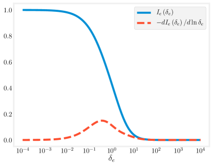
FIG. 6: Function $I_{e}\left(\delta_{e}\right)$ defined by Eq. (36) and negative of its logarithmic derivative $dI_{e}\left(\delta_{e}\right)/d\ln\delta_{e}$ versus the collective parameter $\delta_{e}$.

VI Plasma effects during and after the epoch of reionization

VI.1 Plasma corrections to $y$-distortion

After the epoch of recombination, the universe became ionized again during the epoch of reionization. The epoch of reionization took place approximately for the redshifts $z\sim 6-15$ (Zaroubi, 2013). As CMB light passes through newly ionized intergalactic medium (IGM) during the epoch of reionization and, later, postreionization, as it travels through electron plasma of IGM and through plasma of intracluster medium (ICM) of clusters of galaxies, the CMB spectrum experiences scattering on hot electrons ($T_{e}\gg T_{\gamma}$), which results in Compton $y$-distortion. Modern estimates suggest that sky-averaged nonrelativistic contributions to $y$-distortion from ICM, IGM, and reionization are given, respectively, by $\left\langle y\right\rangle_{ICM}=1.58\times 10^{-6}$, $\left\langle y\right\rangle_{IGM}=8.9\times 10^{-8}$, $\left\langle y\right\rangle_{reion}=9.8\times 10^{-8}$ (Hill et al., 2015), making it the largest expected CMB distortion within the $\Lambda$CDM cosmology (Chluba, 2016). Let us derive and estimate corrections from plasma dispersion described by Eq. (33) and from the collective effects described by Eq. (34) to $y$-type distortion. Note that our analysis below is different from the one in Ref. (Colafrancesco et al., 2015) where it was assumed that plasma modified spectrum given by Eq. (9) enters galaxy cluster, and here we assume that blackbody spectrum enters galaxy cluster and experiences change in dispersion relation or change in scattering due to the collective effects while inside it, which leads to the modification of Compton $y$-distortion.

We rewrite Eq. (33) in terms of the normalized frequency $x=\hbar\omega/T_{\gamma}=\left(T_{e}/T_{\gamma}\right)x_{e}$ and using smallness of $T_{\gamma}/T_{e}\ll 1$ and $y\approx n_{e}\sigma_{T}tc\left(T_{e}/m_{e}c^{2}\right)\ll 1$ we keep only $\partial n_{\gamma}/\partial x$ term in the brackets:

$$\frac{\partial n_{\gamma}}{\partial y}=\frac{1}{x\sqrt{x^{2}-a^{2}}}\\ \times\frac{\partial}{\partial x}\left\{\left(x^{2}-a^{2}\right)^{2}\left[\frac{\partial n_{\gamma}}{\partial x}+\frac{T_{\gamma}}{T_{e}}\left(n_{\gamma}+n_{\gamma}^{2}\right)\right]\right\}\\ \approx\frac{1}{x\sqrt{x^{2}-a^{2}}}\frac{\partial}{\partial x}\left[\left(x^{2}-a^{2}\right)^{2}\frac{\partial n_{\gamma}}{\partial x}\right].$$ (38)

Substituting the equilibrium blackbody solution into the right-hand side, we obtain the estimate for the change in photon distribution:

$$\frac{\Delta n_{\gamma}}{y}=\frac{\sqrt{x^{2}-a^{2}}e^{x}}{\left(e^{x}-1\right)^{2}}\left(\frac{x^{2}-a^{2}}{x}\frac{e^{x}+1}{e^{x}-1}-4\right).$$ (39)

For $a=0$, the above equation gives the usual $y$-type distortion with the corresponding change in intensity $\Delta I_{\omega}\left(x\right)=x^{3}\Delta n_{\gamma}\left(x\right)I_{0}$, where $I_{0}=(\hbar/2\pi^{2}c^{2})\left(T^{3}/\hbar^{3}\right)$. For $a\ll x$, it gives:

$$\frac{\Delta n_{\gamma}}{y}=\frac{xe^{x}}{\left(e^{x}-1\right)^{2}}\left(x\frac{e^{x}+1}{e^{x}-1}-4\right)\\ -\frac{a^{2}}{x^{2}}\frac{xe^{x}}{\left(e^{x}-1\right)^{2}}\left(\frac{3}{2}x\frac{e^{x}+1}{e^{x}-1}-2\right),$$ (40)

where the first term is the usual nonrelativistic $y$-distortion and the second term is $O\left(a^{2}/x^{2}\right)$ order plasma correction to it. For completeness we note that, in addition, the same order $O\left(\omega_{p}^{2}/\omega^{2}\right)$ corrections would also be present due to reflection at the cluster boundary. Equations (39) and (40) together with $\Delta I_{\omega}\left(x\right)=x^{3}\Delta n_{\gamma}\left(x\right)I_{0}$ give the shape and value of the plasma modified $y$-distortion.

Similarly, from Eq. (34) we obtain:

$$\frac{\Delta n_{\gamma}}{y}=\frac{xe^{x}}{\left(e^{x}-1\right)^{2}}\left[I_{e}\left(\delta_{e}\right)\left(x\frac{e^{x}+1}{e^{x}-1}-4\right)\right.\\ \left.+2\frac{x^{2}}{x^{2}-a^{2}}\frac{dI_{e}\left(\delta_{e}\right)}{d\ln\delta_{e}}\right].$$ (41)

Based on Fig. 6 we can see that the effect of Eq. (41) is the overall reduction of the effective value of parameter $y$ for such $x$ that $\delta_{e}\gg 1$. This reduction and the effects from plasma dispersion are negligible for relevant parameters, however. Indeed, the ICM of clusters of galaxies have electron plasma with temperature about $T_{e}\approx 10^{7}\>\textrm{K}$ and density $n_{e}\approx 10^{-4}-10^{-2}\>\textrm{c$\textrm{m}^{-3}$}$ (Sarazin, 1992). We would take $n_{e}\approx 10^{-2}\>\textrm{c$\textrm{m}^{-2}$}$ for estimates, which gives $\omega_{p}\approx 6\times 10^{3}\>\textrm{$\textrm{s}^{-1}$}$. For Planck’s spacecraft $\nu_{min}=30\>\textrm{GHz}$ and $\omega_{p}^{2}/\omega^{2}\approx 10^{-15}$, for SKA-LOW $\nu_{min}=50\>\textrm{MHz}$ and $\omega_{p}^{2}/\omega^{2}\approx 4\times 10^{-10}$. As for the collective plasma correction to $y$-distortion, for Planck’s spacecraft we have $\delta_{e}=8\times 10^{-16}$ and the correction estimated as $\left|1-I_{e}\left(\delta_{e}\right)\right|+0.5\left|dI_{e}\left(\delta_{e}\right)/d\ln\delta_{e}\right|$ is approximately $2\times 10^{-15}$, for SKA-LOW $\delta_{e}=3\times 10^{-10}$ and the correction is about $9\times 10^{-10}$. The collective plasma corrections to $y$-distortion in IGM should be somewhat higher because of the lower temperature, but lower temperature in turn makes the total distortion smaller (parameter $y$), making it harder to detect.

Thus, plasma effects would cause extremely small change, at the order of less than $10^{-10}$, to the already quite small and not yet detected $y$-distortion ($y\approx 10^{-6}$), which makes us conclude that plasma effects on $y$-type distortion during and after the epoch of reionization can hardly be detected in the near future.

A smaller Compton $y$-distortion with $y\approx 10^{-10}-10^{-8}$ also took place for redshift between $z=10^{5}$ and $z=10^{3}$ (Khatri and Sunyaev, 2012) and the same procedure can be applied to those conditions. It is obvious, though, that one would get similarly minuscule corrections.

VI.2 Heating and magnetic field generation

Unlike cosmological recombination, which is mostly a volumetric uniform process, cosmological reionization is a patchy nonuniform process. The universe became reionized because of ultraviolet (UV) light coming from first stars and galaxies (and maybe x-rays coming from quasars) (McQuinn, 2016). This UV light first ionized overdense regions and then ionization fronts were moving ionizing the rest of IGM (Loeb, 2011).

In Refs. (Jiang, 1973; Wilks et al., 1988; Qu et al., 2018) it was shown that, when a plane electromagnetic wave of frequency $\omega_{0}$ experiences sudden ionization, it is transformed into three modes: forward and backward propagating frequency upshifted ($\omega=\sqrt{\omega_{p}^{2}+\omega_{0}^{2}}$) waves, and a static magnetic field mode. It is easy to see that, in case of unpolarized light, there will be no static magnetic field mode since the magnetic fields generated for each equally possible configurations will cancel each other, resulting in heat.

Due to Thomson scattering CMB radiation is linearly polarized at the level of 10% (Buzzelli et al., 2016; Hu and White, 1997). The linear polarization was first detected by the Degree Angular Scale Interferometer (DASI) in 2002 (Kovac et al., 2002). The polarization could be formed at the epoch of recombination (Buzzelli et al., 2016; Kaiser, 1983), i.e., way before the epoch of reionization, so that CMB was likely already polarized just before the ionization. Thus, part of the energy of this linearly polarized component could have been transformed into the energy of static magnetic field. Let us estimate the magnitude of this field.

According to Refs. (Wilks et al., 1988; Qu et al., 2018), the amount of the initial wave energy converted into the magnetic field due to instantaneous ionization is given by

$$\frac{1}{2}\frac{\omega_{p}^{2}}{\omega_{p}^{2}+\omega_{0}^{2}}=\frac{1}{2}\frac{a^{2}}{a^{2}+x^{2}}\approx\frac{1}{2}\frac{a^{2}}{x^{2}},$$ (42)

so that the amount of CMB energy density converted into the magnetic field energy density can be estimated as

$$\frac{B^{2}}{8\pi}\approx 0.1\frac{T^{4}}{\pi^{2}\hbar^{3}c^{3}}\int_{0}^{\infty}\frac{a^{2}}{2x^{2}}\frac{x^{3}}{e^{x}-1}dx=\frac{a^{2}}{8\pi^{2}}\frac{4}{c}\sigma_{SB}\left(\frac{T}{k_{B}}\right)^{4}.$$ (43)

The CMB temperature for $z\sim 6-15$ was approximately $T/k_{B}\sim 19-44\>{\textstyle\textrm{K}}$. Taking $T/k_{B}\approx 20\>\textrm{K}$ and the parameter $a\approx 2\times 10^{-10}$ for this temperature and $n_{e}\approx 10^{-4}\>\textrm{c$\textrm{m}^{-3}$}$ (Inoue, 2004), we get that, even though a very small fraction $a^{2}/8\pi^{2}\approx 5\times 10^{-22}$ of the original CMB energy density goes into the magnetic field energy, we still get cosmologically very large estimates: the magnetic field energy density is at the order of $10^{-30}\>\textrm{erg$\cdot$c$\textrm{m}^{-3}$}$ and the corresponding magnetic field is about $B\approx 10^{-15}\>\textrm{G}$. For comparison, in Ref. (Gnedin et al., 2000) the magnetic field produced during reionization by the Biermann battery effect was estimated to be $B\approx 10^{-19}\>\textrm{G}$. Thus, it seems that the presented mechanism could have been a reason for the origin of the still unexplained initial magnetic field seed (Widrow, 2002; Munirov and Fisch, 2017). However, when we take into account the finite time of ionization $\tau_{ion}$, we find that the ionization happens in the adiabatic regime ($\omega\gg\tau_{ion}^{-1}$), so most of this energy is converted into heat instead of magnetic field. The physical picture is that, in case of sudden ionization, electrons start oscillating approximately at the same phase resulting in the directed motion, electric current, and magnetic field, while for adiabatic ionization electrons have random phases resulting in random motion and heat. The decrease of the magnetic energy with the growth of the ionization time and its conversion into the heat is confirmed by numerical simulations (Wilks et al., 1988).

The ionization time depends on the thickness of the ionization front and can be estimated as $\tau_{ion}=d/v_{front}$, where $d$ is the ionization front thickness and $v_{front}$ is the ionization front speed. According to Ref. (Deparis et al., 2019), the front speed is about $v_{front}\sim\left(0.05-0.1\right)c$. The width of the ionization front can be estimated to be several mean free paths of UV photons (Cantalupo and Porciani, 2011; Lee et al., 2016). The mean free path is around $\lambda_{mfp}\sim 1$ physical kpc. The amount of energy going into the magnetic field exponentially decreases with the growth of the ionization time $\tau_{ion}$ as $\propto e^{-\tau_{ion}\omega}.$ Then, even for low frequencies around plasma frequency $\omega_{p}\approx 5\times 10^{2}\>\textrm{$\textrm{s}^{-1}$}$, $\tau_{ion}\omega_{p}\gg 1$ and the attenuation factor is practically zero $e^{-\tau_{ion}\omega_{p}}\approx 0$, the magnetic field is practically zero, too, with all the energy going into heat. The total amount going into heat is higher by about one order of magnitude if we account for the unpolarized part of CMB light and is roughly $a^{2}/\pi^{2}\approx 10^{-21}$, which gives a tiny temperature increase of about $\triangle T/k_{B}\approx 10^{-20}\>{\textstyle\textrm{K}}$.

The possibility of the generation of seed magnetic field should not be completely ruled out, however. For example, regions with higher than average density and, consequently, higher parameter $a$ can be present or sharper ionization fronts can be potentially produced.

VII Summary and conclusions

We derived, using three different approaches, the equilibrium radiation spectrum inside plasma. We demonstrated that, because of dispersion, it is different from the blackbody Planck spectrum. We considered what stationary and moving observers sent into the plasma-filled universe would measure and how these results should be interpreted.

We then considered how plasma can affect the spectrum of CMB radiation. Namely, we pointed out the change in the cosmological redshift that can appear as an effective frequency-dependent chemical potential; we discussed the possibility of the direct detection of plasma equilibrium spectrum from CMB data, emphasized its sensitivity to how fast the cosmological recombination happened and reached more pessimistic conclusion about its experimental detection than before (Colafrancesco et al., 2015); we gave expressions for the modified Kompaneets equation due to plasma dispersion and collective effects; we calculated how Compton $y$-distortion during and after the epoch of reionization is changed because of plasma; and we proposed, estimated, and deemed likely unrealistic a novel mechanism of magnetic field generation during the epoch of reionization due to conversion of some of the energy of CMB into magnetic field energy.

We concluded that plasma effects are extremely small, on the order of $O\left(\omega_{p}^{2}/\omega^{2}\right)$ in most cases and hence cannot be realistically detected in the near future. However, if some of the assumptions employed here were violated, then there would be possibilities for larger effects. Thus, it is important to know how plasma affects the CMB spectrum in order to fully understand the cosmological evolution of our universe; for example, restrictions imposed by plasma effects might, in principle, be used to test alternative models of cosmology as they put boundaries on the baryon density at different epochs. Moreover, the analysis conducted in the paper could be relevant to other astrophysical and laboratory situations where radiation interacts with plasma.

References

- Tauber et al. (2010) J. A. Tauber, N. Mandolesi, J.-L. Puget, T. Banos, M. Bersanelli, F. R. Bouchet, R. C. Butler, J. Charra, G. Crone, J. Dodsworth, et al., A&A 520, A1 (2010).
- Dewdney et al. (2013) P. Dewdney, W. Turner, R. Millenaar, R. McCool, J. Lazio, and T. Cornwell, Document number SKA-TEL-SKO-DD-001 Revision 1 (2013).
- Huang (1987) K. Huang, Statistical Mechanics, 2nd Edition (Wiley, New York, 1987).
- Greiner et al. (1995) W. Greiner, L. Neise, and H. Stöcker, Thermodynamics and statistical mechanics, Classical theoretical physics (Springer-Verlag, New York, 1995).
- Wurfel (1982) P. Wurfel, Journal of Physics C: Solid State Physics 15, 3967 (1982).
- Herrmann and Würfel (2005) F. Herrmann and P. Würfel, American Journal of Physics 73, 717 (2005).
- Ries and McEvoy (1991) H. Ries and A. McEvoy, Journal of Photochemistry and Photobiology A: Chemistry 59, 11 (1991).
- Markvart (2008) T. Markvart, Journal of Optics A: Pure and Applied Optics 10, 015008 (2008).
- Zel’dovich and Levich (1969) Y. B. Zel’dovich and E. Levich, Sov. Phys. JETP 28, 1287 (1969).
- Klaers et al. (2010) J. Klaers, F. Vewinger, and M. Weitz, Nature Physics 6, 512 EP (2010).
- Klaers (2014) J. Klaers, Journal of Physics B: Atomic, Molecular and Optical Physics 47, 243001 (2014).
- Hafezi et al. (2015) M. Hafezi, P. Adhikari, and J. M. Taylor, Phys. Rev. B 92, 174305 (2015).
- Wang et al. (2018) C.-H. Wang, M. J. Gullans, J. V. Porto, W. D. Phillips, and J. M. Taylor, Phys. Rev. A 98, 013834 (2018).
- Meyer and Markvart (2009) T. J. J. Meyer and T. Markvart, Journal of Applied Physics 105, 063110 (2009).
- Reiser and Schächter (2013) A. Reiser and L. Schächter, Phys. Rev. A 87, 033801 (2013).
- Sokolsky and Gorlach (2014) A. A. Sokolsky and M. A. Gorlach, Phys. Rev. A 89, 013847 (2014).
- McGregor (1978) W. McGregor, Journal of Quantitative Spectroscopy and Radiative Transfer 19, 659 (1978).
- Bannur (2006) V. M. Bannur, Phys. Rev. E 73, 067401 (2006).
- Trigger (2007) S. Trigger, Physics Letters A 370, 365 (2007).
- Triger and Khomkin (2010) S. A. Triger and A. L. Khomkin, Plasma Physics Reports 36, 1095 (2010).
- Medvedev (1999) M. V. Medvedev, Phys. Rev. E 59, R4766 (1999).
- Tsintsadze et al. (1996) L. N. Tsintsadze, D. K. Callebaut, and N. L. Tsintsadze, Journal of Plasma Physics 55, 407 (1996).
- Mati (2019) P. Mati, arXiv e-prints , arXiv:1902.07998 (2019), arXiv:1902.07998 [cond-mat.stat-mech] .
- Chen and Lin (2003) J. Chen and B. Lin, Journal of Physics A: Mathematical and General 36, 11385 (2003).
- Bohren and Huffman (1983) C. F. Bohren and D. R. Huffman, Absorption and scattering of light by small particles (Wiley, New York, 1983).
- Massoud (2005) M. Massoud, Engineering thermofluids, Vol. 2005 (Springer, Berlin, Heidelberg, 2005).
- Greffet et al. (2018) J.-J. Greffet, P. Bouchon, G. Brucoli, and F. Marquier, Phys. Rev. X 8, 021008 (2018).
- Lifshitz and Pitaevskii (1980) E. Lifshitz and L. Pitaevskii, Course of Theoretical Physics: Statistical Physics, Part 2 (Pergamon Press, 1980).
- Bekefi (1966) G. Bekefi, Radiation Processes in Plasmas (Wiley, 1966).
- Zheleznyakov (1996) V. V. Zheleznyakov, Radiation in Astrophysical Plasmas (Kluwer Academic, 1996).
- Bičák and Hadrava (1975) J. Bičák and P. Hadrava, Astronomy and Astrophysics 44, 389 (1975).
- Fixsen (2009) D. J. Fixsen, The Astrophysical Journal 707, 916 (2009).
- Colafrancesco et al. (2015) S. Colafrancesco, M. S. Emritte, and P. Marchegiani, Journal of Cosmology and Astroparticle Physics 2015 (05), 006.
- Howell and Shakeshaft (1967) T. F. Howell and J. R. Shakeshaft, Nature 216, 753 EP (1967).
- Sironi et al. (1990) G. Sironi, M. Limon, G. Marcellino, G. Bonelli, M. Bersanelli, G. Conti, and K. Reif, Astrophys. J. 357, 301 (1990).
- Sironi et al. (1991) G. Sironi, G. Bonelli, and M. Limon, Astrophys. J. 378, 550 (1991).
- Sunyaev and Chluba (2009) R. Sunyaev and J. Chluba, Reviews in Modern Astronomy 21, 1 (2009).
- Dodin and Fisch (2010a) I. Y. Dodin and N. J. Fisch, Physics of Plasmas 17, 112113 (2010a).
- Chluba and Ali-Haïmoud (2016) J. Chluba and Y. Ali-Haïmoud, Monthly Notices of the Royal Astronomical Society 456, 3494 (2016).
- Chluba (2016) J. Chluba, Monthly Notices of the Royal Astronomical Society 460, 227 (2016).
- Dodin and Fisch (2010b) I. Y. Dodin and N. J. Fisch, Phys. Rev. D 82, 044044 (2010b).
- Khatri and Sunyaev (2012) R. Khatri and R. A. Sunyaev, Journal of Cosmology and Astroparticle Physics 2012 (06), 038.
- Kompaneets (1957) A. Kompaneets, Sov. Phys. JETP 4, 730 (1957).
- Fixsen et al. (1996) D. J. Fixsen, E. S. Cheng, J. M. Gales, J. C. Mather, R. A. ShaFer, and E. L. Wright, The Astrophysical Journal 473, 576 (1996).
- Khatri and Sunyaev (2015) R. Khatri and R. Sunyaev, Journal of Cosmology and Astroparticle Physics 2015 (09), 026.
- Tashiro (2014) H. Tashiro, Progress of Theoretical and Experimental Physics 2014, 06B107 (2014).
- Mendonça and Terças (2017) J. T. Mendonça and H. Terças, Phys. Rev. A 95, 063611 (2017).
- Zel’dovich (1975) Y. B. Zel’dovich, Phys. Usp. 18, 79 (1975).
- Khatri et al. (2012) R. Khatri, R. A. Sunyaev, and J. Chluba, Astronomy and Astrophysics 540, A124 (2012).
- Bingham et al. (2003) R. Bingham, V. N. Tsytovich, U. de Angelis, A. Forlani, and J. T. Mendonça, Physics of Plasmas 10, 3297 (2003).
- Zaroubi (2013) S. Zaroubi, The epoch of reionization, in The First Galaxies: Theoretical Predictions and Observational Clues, edited by T. Wiklind, B. Mobasher, and V. Bromm (Springer Berlin Heidelberg, Berlin, Heidelberg, 2013) pp. 45–101.
- Hill et al. (2015) J. C. Hill, N. Battaglia, J. Chluba, S. Ferraro, E. Schaan, and D. N. Spergel, Phys. Rev. Lett. 115, 261301 (2015).
- Sarazin (1992) C. L. Sarazin, The intracluster medium, in Clusters and Superclusters of Galaxies, edited by A. C. Fabian (Springer Netherlands, Dordrecht, 1992) pp. 131–150.
- McQuinn (2016) M. McQuinn, Annual Review of Astronomy and Astrophysics 54, 313 (2016).
- Loeb (2011) A. Loeb, The reionization of cosmic hydrogen by the first galaxies, in Adventures in Cosmology (WORLD SCIENTIFIC, 2011) pp. 41–88.
- Jiang (1973) C.-L. Jiang, Electromagnetic wave propagation and radiation in a suddenly created plasma, Ph.D. thesis, California Institute of Technology (1973).
- Wilks et al. (1988) S. C. Wilks, J. M. Dawson, and W. B. Mori, Phys. Rev. Lett. 61, 337 (1988).
- Qu et al. (2018) K. Qu, Q. Jia, M. R. Edwards, and N. J. Fisch, Phys. Rev. E 98, 023202 (2018).
- Buzzelli et al. (2016) A. Buzzelli, P. Cabella, G. de Gasperis, and N. Vittorio, Journal of Physics: Conference Series 689, 012003 (2016).
- Hu and White (1997) W. Hu and M. White, New Astronomy 2, 323 (1997).
- Kovac et al. (2002) J. M. Kovac, E. M. Leitch, C. Pryke, J. E. Carlstrom, N. W. Halverson, and W. L. Holzapfel, Nature 420, 772 EP (2002).
- Kaiser (1983) N. Kaiser, Monthly Notices of the Royal Astronomical Society 202, 1169 (1983).
- Inoue (2004) S. Inoue, Monthly Notices of the Royal Astronomical Society 348, 999 (2004).
- Gnedin et al. (2000) N. Y. Gnedin, A. Ferrara, and E. G. Zweibel, The Astrophysical Journal 539, 505 (2000).
- Widrow (2002) L. M. Widrow, Rev. Mod. Phys. 74, 775 (2002).
- Munirov and Fisch (2017) V. R. Munirov and N. J. Fisch, Phys. Rev. E 95, 013205 (2017).
- Deparis et al. (2019) N. Deparis, D. Aubert, P. Ocvirk, J. Chardin, and J. Lewis, A&A 622, A142 (2019).
- Cantalupo and Porciani (2011) S. Cantalupo and C. Porciani, Monthly Notices of the Royal Astronomical Society 411, 1678 (2011).
- Lee et al. (2016) K.-Y. Lee, G. Mellema, and P. Lundqvist, Monthly Notices of the Royal Astronomical Society 455, 4406 (2016).