Harmonic Stability of Standing Water Waves

Abstract.

A numerical method is developed to study the stability of standing water waves and other time-periodic solutions of the free-surface Euler equations using Floquet theory. A Fourier truncation of the monodromy operator is computed by solving the linearized Euler equations about the standing wave with initial conditions ranging over all Fourier modes up to a given wave number. The eigenvalues of the truncated monodromy operator are computed and ordered by the mean wave number of the corresponding eigenfunctions, which we introduce as a method of retaining only accurately computed Floquet multipliers. The mean wave number matches up with analytical results for the zero-amplitude standing wave and is helpful in identifying which Floquet multipliers collide and leave the unit circle to form unstable eigenmodes or rejoin the unit circle to regain stability. For standing waves in deep water, most waves with crest acceleration below $A_{c}=0.889$ are found to be linearly stable to harmonic perturbations; however, we find several bubbles of instability at lower values of $A_{c}$ that have not been reported previously in the literature. We also study the stability of several new or recently discovered time-periodic gravity-capillary or gravity waves in deep or shallow water, finding several examples of large-amplitude waves that are stable to harmonic perturbations and others that are not. A new method of matching the Floquet multipliers of two nearby standing waves by solving a linear assignment problem is also proposed to track individual eigenvalues via homotopy from the zero-amplitude state to large-amplitude standing waves.

1. Introduction

Standing water waves have played a central role in the study of fluid mechanics throughout history. Already in 1831, Faraday observed patterns of ink at the surface of milk driven by a tuning fork [33]. He noticed that the waves oscillate at half the forcing frequency, which was later explained by Rayleigh [73]. Benjamin and Ursell performed a linear stability analysis in [9], which was later extended to viscous fluids by Kumar and Tuckerman [48]. Additional theoretical, numerical and experimental studies of Faraday waves include [99, 78, 90, 98, 18, 60, 63, 69, 36, 44, 13].

Standing waves at the surface of an inviscid fluid with no external driving force have also been studied extensively. Building on the asymptotic techniques developed by Stokes for traveling waves [80], Rayleigh showed how to incorporate time-evolution in the analysis and computed standing waves to third order [72]. Penney and Price extended Rayleigh’s expansion to 5th order and conjectured the existence of an extreme standing wave that forms a 90 degree corner each time the wave comes to rest [68]. Taylor confirmed experimentally that large-amplitude standing waves nearly form 90 degree corners [83] but was skeptical of Penney and Price’s mathematical argument. Tadjbakhsh and Keller [82] and Concus [20] incorporated finite-depth and surface tension effects in the asymptotic expansions. Concus later realized there were small-divisor issues that called into question the validity of the asymptotic techniques that had been developed to study standing waves up to that point [21]. It took 40 years for these issues to be sorted out using Nash-Moser theory [70, 42, 1]. Along the way, asymptotic expansions to arbitrary order were computed for standing waves in deep water by Schwartz and Whitney [77] and a semi-analytic theory of standing waves was proposed by Amick and Toland [2]. On the computational side, Mercer and Roberts [56, 57], Tsai and Jeng [85], Bryant and Stiassnie [12], Schultz et al. [75], Okamura [65, 66], Wilkening [93], Wilkening and Yu [97], and many others have developed numerical algorithms for computing standing water waves. Due to the difficulty of maintaining accuracy in nearly singular free-surface flow calculations, different conclusions were reached by these authors regarding the form of the largest-amplitude standing wave. The question was finally settled in [93, 97], where it was shown that the Penney-Price conjecture is false due to a breakdown in self-similarity at the crests of very large-amplitude standing waves.

While much is known about the stability of traveling water waves [8, 7, 50, 51, 27, 54, 43, 61, 29, 84], relatively little work has been done on the stability of standing waves. The most comprehensive study to date is by Mercer and Roberts [56], who found that standing waves on deep water are linearly stable to harmonic perturbations for crest acceleration in the range $0\leq A_{c}\leq 0.889$. (Crest acceleration is the downward acceleration of a fluid particle at the wave crest at maximum height when the fluid comes to rest, relative to the gravitational acceleration.) They also studied subharmonic perturbations with wavelength equal to 8 times the fundamental wavelength of the standing wave, finding sideband instabilities in which the base wave (mode $m=8$) interacts with modes $m\pm l$, with $l$ an integer. Bryant and Stiassnie [12] found that sideband instabilities lead to cyclic recurrence over hundreds of periods of the basic standing wave when evolved numerically on a domain containing 9 replicas of the standing wave. Bridges and Laine-Pearson [11] have shown that the modulational instability of standing waves is closely linked to that of the component counter-propagating traveling waves at the weakly nonlinear level for a wide range of Hamiltonian PDEs, including water waves. In the present work we focus on harmonic stability, which is natural in the context of standing waves in a container with vertical walls. Subharmonic stability of more general “traveling-standing” waves will be considered elsewhere [96].

To determine the stability of standing waves and other time-periodic solutions of the free-surface Euler equations to harmonic perturbations, we compute Floquet multipliers of the monodromy operator to determine if they lie on the unit circle. The main difference between our approach and that of Mercer and Roberts [56] is that we employ a Fourier basis rather than discrete delta functions. This has a computational advantage in that only the leading columns of the monodromy operator need be computed; thus, the mesh can be refined independently of the size of the (truncated) operator so that all the matrix entries are accurate. We also order the eigenvalues according to the “mean wave number” of the corresponding eigenfunctions, which turns out to be closely correlated with the residual error of the eigenpair. By parallelizing the computation of the operator using a GPU, we are able to increase the number of Floquet multipliers that can be computed by 2 orders of magnitude over previous studies. Doing this reveals additional bubbles of instability [54] in the range $0\leq A_{c}\leq 0.889$, previously thought to contain only stable solutions.

In addition to studying the stability of standing waves in deep water, we consider for the first time finite depth and capillary effects on stability. In infinite depth, standing waves involve large-scale motion of the bulk fluid. However, in shallow water, they are better described as counter-propagating solitary waves that repeatedly collide with one another. We consider a particular family of standing waves with wavelength $2\pi$ and fluid depth $h=0.05$. We find examples of waves well outside of the weakly nonlinear regime that are stable to harmonic perturbations, and another that is unstable. We also study the stability of gravity-capillary waves. These can take the form of counter-propagating depression waves, for which we give an example of a large-amplitude wave that is stable to harmonic perturbations. We also search for a new type of time-periodic water wave consisting of counter-propagating gravity-capillary solitary waves [52, 88, 58] that collide repeatedly with each other. We present two such waves, one that is stable to harmonic perturbations and one that is unstable.

A technical challenge that arises in studying the stability of standing waves is that the Floquet multipliers are complex numbers whose phase is only known modulo $2\pi$; thus, while they mostly lie on the unit circle, they are scrambled together. By contrast, for traveling waves, the eigenvalues mostly lie on the imaginary axis and are naturally ordered by their imaginary part. We introduce a “mean wave number” to measure how oscillatory the corresponding eigenfunctions are, and use this to order the eigenvalues. This aids in discarding inaccurate eigenvalues and also proves useful in identifying which eigenvalues collide and leave the unit circle to form unstable eigenmodes or rejoin the unit circle to regain stability. In order to track individual eigenvalues via a homotopy method, we propose an algorithm to match the Floquet multipliers of nearby standing waves by solving a linear assignment problem. The mean wave number also plays a role in the cost matrix of this assignment problem.

This paper is organized as follows. In Section 2 we discuss the free-surface Euler equations, non-uniform meshes, symmetry, and our overdetermined shooting method for computing time-periodic solutions. In Section 3, we discuss linearization about time-periodic solutions, Hamiltonian time reversal, and a Fourier basis for computing the monodromy operator efficiently. We also analyze the stability of the zero-amplitude solution and present our numerical algorithm for computing Floquet multipliers. In Section 4.1 we study the stability of standing waves in deep water with crest acceleration in the range $0\leq A_{c}\leq 0.9639$. Like Mercer and Roberts [56], we find that there is a critical bifurcation at $A_{c}=0.889$ beyond which all standing waves are unstable. However, we also find new bubbles of instability below this critical threshold and investigate one of them in detail. In Section 4.2 we discuss the numerical splitting of the $\lambda=1$ eigenvalue due to Jordan chains associated with translation in time and space. In Section 4.3, we study the stability of counter-propagating solitary waves in shallow water, including large-amplitude time-periodic waves that temporarily form a jet that is taller than the fluid depth. In Section 4.4, we study the stability of two types of gravity-capillary waves in deep water. The first type consists of counter-propagating depression waves that bifurcate from the flat rest state as predicted by Concus [20]. The second is a new type of time-periodic wave constructed from two counter-propagating solitary waves [52, 88, 58] with initial conditions tuned to achieve time-periodicity. The appendices describe (A) the boundary integral formulation; (B) a method of computing traveling waves using the overdetermined shooting method; (C) computation of the Jacobian and the state transition matrix; and (D) a linear assignment problem for matching eigenvalues at adjacent values of $A_{c}$ to track eigenvalues via homotopy from the zero-amplitude state to large-amplitude standing waves.

2. Preliminaries: computation of standing water waves

In this section, we describe an overdetermined shooting algorithm for computing time-periodic solutions of the free-surface Euler equations with spectral accuracy. We build on this method in Section 3 to compute the monodromy operator and its eigenvalues, which determine whether the underlying solution is linearly stable to harmonic perturbations. We also use the method in Section 4.4 to compute new families of time-periodic gravity-capillary waves and investigate their stability. The overdetermined shooting algorithm is explained in more detail in Wilkening and Yu [97], and builds on previous shooting methods [56, 57, 75, 79]. Other successful approaches for computing standing waves include Fourier collocation in space and time [86, 85, 65, 67, 66] and semi-analytic series expansions [77, 2].

2.1. Equations of motion

The equations of motion of a free surface $\eta(x,t)$ evolving over an ideal fluid with velocity potential $\phi(x,y,t)$ may be written [91, 45, 25, 26]

$$\eta_{t} =\phi_{y}-\eta_{x}\phi_{x},$$ (2.1)

$$\varphi_{t} =P\left[\phi_{y}\eta_{t}-\frac{1}{2}\phi_{x}^{2}-\frac{1}{2}\phi_{y}^{2}-g\eta+\frac{\sigma}{\rho}\partial_{x}\left(\frac{\eta_{x}}{\sqrt{1+\eta_{x}^{2}}}\right)\right],$$

where subscripts denote partial derivatives, $\varphi(x,t)=\phi(x,\eta(x,t),t)$ is the restriction of $\phi$ to the free surface, $g$ is the acceleration of gravity, $\rho$ is the fluid density, $\sigma\geq 0$ is the surface tension (possibly zero), and $P$ is the $L^{2}$-projection to zero mean that annihilates constant functions,

$$P=\operatorname{id}-P_{0},\qquad P_{0}f=\frac{1}{2\pi}\int_{0}^{2\pi}f(x)\,dx.$$ (2.2)

Here we have non-dimensionalized the equations so that the wavelength of the standing wave is $2\pi$. In physical variables, (2.1) still describes the dynamics if we put tildes over $\eta$, $\phi$, $\varphi$, $x$, $y$, $t$, $g$, $\sigma$ and $\rho$ and modify $P_{0}$ to compute the mean over $[0,2\pi L]$, where

$$\tilde{\eta}(\tilde{x},\tilde{t})=L\eta\left(\frac{\tilde{x}}{L},\frac{\tilde{t}}{\tau}\right),\quad\tilde{\phi}(\tilde{x},\tilde{y},\tilde{t})=\frac{L^{2}}{\tau}\phi\left(\frac{\tilde{x}}{L},\frac{\tilde{y}}{L},\frac{\tilde{t}}{\tau}\right),\quad\tilde{g}=\frac{L}{\tau^{2}}g,\quad\frac{\tilde{\sigma}}{\tilde{\rho}}=\frac{L^{3}}{\tau^{2}}\frac{\sigma}{\rho}.$$ (2.3)

Here $L$ and $\tau$ are the physical length and time corresponding to one unit of dimensionless length and time, respectively. The projection $P$ yields a convenient convention for selecting the arbitrary additive constant in the potential, and has no effect (barring roundoff errors and discretization errors) if the fluid has infinite depth and the mean surface height is zero. The velocity components $u=\phi_{x}$ and $v=\phi_{y}$ at the free surface can be computed from $\varphi$ via

$$\begin{pmatrix}\phi_{x}\\ \phi_{y}\end{pmatrix}=\frac{1}{1+\eta^{\prime}(x)^{2}}\begin{pmatrix}1&-\eta^{\prime}(x)\\ \eta^{\prime}(x)&1\end{pmatrix}\begin{pmatrix}\varphi^{\prime}(x)\\ \mathcal{G}\varphi(x)\end{pmatrix},$$ (2.4)

where a prime denotes a derivative and $\mathcal{G}$ is the Dirichlet-Neumann operator [24]

$$\mathcal{G}\varphi(x)=\sqrt{1+\eta^{\prime}(x)^{2}}\,\,\frac{\partial\phi}{\partial n}(x+i\eta(x))$$ (2.5)

for the Laplace equation, with periodic boundary conditions in $x$, $\phi=\varphi$ on the upper boundary, and $\phi_{y}=0$ at $y=-\infty$ or at $y=-h$ in the finite depth case. We have suppressed $t$ in the notation as time is frozen when solving the Laplace equation. We compute $\mathcal{G}\varphi$ using a boundary integral collocation method; see Appendix A.

This method is flexible enough to allow for non-uniform meshes in space and time. We adopt a simple approach in which time is divided into $\nu$ segments of relative size $\theta_{l}$, where $\theta_{1}+\theta_{2}+\cdots+\theta_{\nu}=1$. We take $N_{l}$ uniformly spaced timesteps on segment $l$. The spatial grid on this time segment is fixed, with two parameters $\kappa_{l}\in\mathbb{Z}$ and $\rho_{l}\in(0,1]$ controlling the relative grid spacing near $x=0$ and $x=\pi$. The spatial grid on segment $l$ is $x_{i}=\xi_{l}(\alpha_{i})$, where $\alpha_{i}=2\pi i/M_{l}$ for $0\leq i<M_{l}$ and

$$\xi_{l}(\alpha)=\int_{0}^{\alpha}E_{l}(\beta)\,d\beta,\qquad\quad E_{l}(\alpha)=\left\{\begin{array}[]{rl}\!\!1-A_{l}\big{[}\sin^{2\kappa_{l}}(\alpha/2)-\mu_{l}\big{]},&\kappa_{l}>0,\!\!\\[2.0pt] \!\!1,&\kappa_{l}=0,\!\!\\ \!\!1-A_{l}\big{[}\cos^{2|\kappa_{l}|}(\alpha/2)-\mu_{l}\big{]},&\kappa_{l}<0.\!\!\end{array}\right.$$ (2.6)

Here  $\displaystyle\mu_{l}=\frac{(2|\kappa_{l}|-1)!!}{(2|\kappa_{l}|)!!}=\frac{\Gamma(|\kappa_{l}|+\frac{1}{2})}{\sqrt{\pi}\,\,\Gamma(|\kappa_{l}|+1)}$ and  $\displaystyle A_{l}=\frac{1-\rho_{l}}{1-\mu_{l}(1-\rho_{l})}$  are chosen so that

$$\xi_{l}(2\pi)=2\pi,\qquad\quad\frac{\min\{E_{l}(0),E_{l}(\pi)\}}{\max\{E_{l}(0),E_{l}(\pi)\}}=\rho_{l}.$$ (2.7)

Mesh refinement near $x=0$ or $x=\pi$ causes the grid to sparsen near $x=\pi$ or $x=0$ by a factor of $\displaystyle\max\{E_{l}(0),E_{l}(\pi)\}=1+A_{l}\mu_{l}=1/[1-\mu_{l}(1-\rho_{l})]$ relative to a uniform grid. Note that $\kappa_{l}=0$ is a separate case in (2.6) and corresponds to uniform spacing. For nonzero $\kappa_{l}$, the mesh is uniform when $\rho_{l}=1$ and becomes increasingly concentrated near the center ($\kappa_{l}>0$) or endpoints ($\kappa_{l}<0$) as $\rho_{l}$ decreases toward 0. Larger values of $|\kappa_{l}|$ lead to more localized regions of mesh refinement. In the present paper, we use either $\kappa_{l}=0$ (uniform spacing), $\kappa_{l}=2$ (mesh refinement near $x=\pi$), or $\kappa_{l}=-2$ (mesh refinement near $x=0,2\pi$). Re-spacing the grid from segment $l$ to $l+1$ amounts to interpolating the values of $\eta$ and $\varphi$ from the old mesh to the new mesh. We do this by solving e.g. $\eta\circ\xi_{l+1}(\alpha_{j})=\eta\circ\xi_{l}(\xi_{l}^{-1}\circ\xi_{l+1}(\alpha_{j}))$ by Newton’s method.

For time-stepping (2.1), we use a 5th or 8th order Runge-Kutta scheme [35] in double-precision and a 15th order spectral deferred correction method [31, 41, 49, 71] in quadruple-precision (SDC15). We also make use of the 36th order filter popularized by Hou, Lowengrub and Shelley [38, 39, 40, 37]. This filter consists of multiplying the $k$th Fourier mode by

$$\exp\left[-36\big{(}|k|/k_{\text{max}}\big{)}^{36}\right],\qquad k_{\text{max}}=M/2,$$ (2.8)

which strikes a balance between suppressing aliasing errors and resolving high-frequency modes. Here $M=M_{l}$ is the number of grid points used on the $l^{\text{th}}$ spatial grid.

2.2. Symmetry

To compute symmetric standing waves [68, 82, 20], we exploit a symmetry that reduces the computation time by a factor of four [56, 97]. In order for the solution to return to its initial state at time $T$, it suffices to reach a rest state in which

$$\varphi(x,T/4)=0,\qquad 0\leq x\leq 2\pi,$$ (2.9)

provided $\eta(x,0)$ and $\varphi(x,0)$ are spatially periodic even functions satisfying

$$\eta(x+\pi,0)=\eta(x,0),\quad\varphi(x+\pi,0)=-\varphi(x,0).$$ (2.10)

Indeed, reversing time about $t=T/4$ merely changes the sign of $\varphi$, due to (2.9). Thus, $\eta(x,T/2)=\eta(x,0)$ and $\varphi(x,T/2)=-\varphi(x,0)$, i.e. the wave profile at $T/2$ is identical to its initial configuration, while the velocity potential changes sign. By (2.10), the evolution from $T/2$ to $T$ will be the same as that from $0$ to $T/2$ with a spatial translation by $\pi$. Using (2.10) again shows that $\eta(x,T)=\eta(x,0)$ and $\varphi(x,T)=\varphi(x,0)$, i.e. the solution is time-periodic.

Once the initial conditions and period are found using symmetry to accelerate the search for standing waves, we double-check that the numerical solution evolved from $0$ to $T$ is indeed time-periodic. Our Floquet analysis of the stability of these solutions is also performed over the entire interval, $[0,T]$.

2.3. Trust-region minimization

Following Wilkening and Yu [97], we compute time-periodic solutions in a shooting framework by posing the problem as an overdetermined nonlinear system of equations. The system is overdetermined because we only solve for the leading Fourier modes of the initial conditions, zero-padding the rest, but still impose time-periodicity on all the Fourier modes. This improves robustness over more traditional shooting methods and enables us to compute sensitivities by discretizing linearized equations rather than linearizing the discrete nonlinear equations. This allows us to share the data structure for the Dirichlet-Neumann operator across all columns of the Jacobian calculation, leading to a very efficient parallel code framework.

Let $\hat{\eta}_{k}(t)$ and $\hat{\varphi}_{k}(t)$ denote the Fourier modes of the solution. For symmetric standing waves, we assume the initial conditions have the form

$$\hat{\eta}_{k}(0) =c_{|k|},\qquad(k=\pm 2,\pm 4,\pm 6,\dots\;;\;|k|\leq n),$$ (2.11)

$$\hat{\varphi}_{k}(0) =c_{|k|},\qquad(k=\pm 1,\pm 3,\pm 5,\dots\;;\;|k|\leq n),$$

where $c_{1},\dots,c_{n}$ are real numbers, and all other Fourier modes are zero. If the fluid depth is finite, we also set $\hat{\eta}_{0}=h$, where $h$ is the mean fluid depth. The integer $n$ controls the cutoff beyond which the Fourier modes are zero-padded. We normally choose $n$ in the range $M/6\leq n\leq M/3$, where $M$ is the number of grid points. We also set

$$c_{0}=T,$$ (2.12)

the unknown period. We then define the objective function

$$f(c) =\frac{1}{2}r(c)^{T}r(c)\approx\frac{1}{4\pi}\int_{0}^{2\pi}\varphi(x,T/4)^{2}\,dx,$$ (2.13)

$$r_{j} =\varphi(\alpha_{j},T/4)/\sqrt{M},\qquad\alpha_{j}=2\pi j/M,\qquad 0\leq j<M.$$

As explained in Section 2.2 above, driving $f$ to zero will yield time-periodic solutions with the symmetry properties expected of standing waves. Note that the number of equations, $m=M$, is generally larger than the number of unknowns, $n$, due to zero-padding of the initial conditions. When computing extreme standing waves using $f$ of the form (2.13), we often refine the mesh as $t$ approaches $T/4$, which further increases $m$ relative to $n$. See Wilkening and Yu [97] for details.

We compute families of time-periodic solutions by specifying the mean fluid depth $h$ (possibly infinite) and one of the parameters $c_{k}$ (with $k=k_{0}$, say) in a continuation algorithm. The other $c_{k}$ with $k\neq k_{0}$ are chosen to minimize the objective function $f$ using a variant of the Levenberg-Marquardt method [97]. The Levenberg-Marquardt method requires a Jacobian matrix $J_{jk}=\partial r_{j}/\partial c_{k}$, which we compute by solving the variational equations, namely (3.5) below, repeatedly, in parallel, with different initial conditions; see Appendix C. If $f$ reaches a local minimum that is higher than a specified threshold (normally $10^{-26}$ in double-precision and $10^{-52}$ in quadruple precision), we try again with a larger $n$, a larger $M$, a value of $c_{k_{0}}$ closer to the last successful attempt, or a different index $k_{0}$. Switching the index is often useful when tracking a fold in the bifurcation curve. In some cases (see sections 4.3 and 4.4 below), rather than freeze the period or a Fourier mode, we specify the value of $\eta(a,0)$ at $a=0$, $a=\pi/2$ or $a=\pi$. This is done by adding a component to $r$, namely

$$r_{m}=\left[\hat{\eta}_{0}+\left(\textstyle\sum_{k=1}^{M/2}\hat{\eta}_{k}(0)\big{[}2\cos(ka)\big{]}\right)-\eta(a,0)\right]w_{m},$$ (2.14)

where $\hat{\eta}_{0}$ and $\eta(a,0)$ are given, $w_{m}$ is a weight (typically $10^{-2}$ or $1$), and $\hat{\eta}_{k}(0)$ is either 0 or one of the $c_{j}$ (hence real). In this approach, none of the $c_{k}$ are frozen and $r(c)$ is a nonlinear function from $\mathbb{R}^{n+1}$ to $\mathbb{R}^{m+1}$.

3. Stability

Once a time-periodic solution is found, we can check its stability using Floquet theory [19]. We restrict attention to harmonic stability here, which is physically reasonable for symmetric standing waves in a tank with vertical walls. Subharmonic stability will be treated in a follow-up paper in the more general context of traveling-standing water waves [96], which include traveling waves and standing waves as special cases.

Let $q(x,t)=\big{(}\eta(x,t);\varphi(x,t)\big{)}$ be a time-periodic solution of the nonlinear system (2.1) with period $T$. Here a semicolon separates the components of a column vector. When convenient, we drop the $x$-dependence in the notation and regard $q(\cdot,t)$ (or simply $q(t)$) as evolving in an abstract Hilbert space such as $L^{2}(\mathbb{T})\times H^{1}(\mathbb{T})$, where $\mathbb{T}=\mathbb{R}\big{/}2\pi\mathbb{Z}$. We write (2.1) abstractly as

$$\partial_{t}q=F(q).$$ (3.1)

The linearized system

$$\partial_{t}\dot{q}=DF(q(t))\dot{q}$$ (3.2)

generates a family of state-transition operators, $E$, such that

$$\dot{q}(t)=E(t,t_{0})\dot{q}_{0}$$ (3.3)

is the solution of (3.2) satisfying $\dot{q}(t_{0})=\dot{q}_{0}$. Note that a dot represents a variational derivative, not a time derivative; see (C.1) in Appendix C. We denote the monodromy operator by

$$E_{T}=E(T,0).$$ (3.4)

It gives the change at time $T$ due to a perturbation at time 0. For $m\in\mathbb{Z}$ we have $E((m+1)T,mT)=E_{T}$ since $DF(q(t))$ is periodic. Formulas for the linearized system (3.2) are given by

$$\dot{\eta}_{t} =\left(\dot{\phi}_{y}-\eta_{x}\dot{\phi}_{x}\right)-\left(\dot{\eta}\phi_{x}\right)^{\prime},$$ (3.5)

$$\dot{\varphi}_{t} =P\left[-\left(\dot{\eta}\phi_{x}\phi_{y}\right)^{\prime}-\phi_{x}\dot{\phi}^{\prime}+\phi_{y}\left(\dot{\phi}_{y}-\eta_{x}\dot{\phi}_{x}\right)-g\dot{\eta}+\frac{\sigma}{\rho}\partial_{x}\left(\frac{\dot{\eta}_{x}}{(1+\eta_{x}^{2})^{3/2}}\right)\right],$$

where the right-hand side is evaluated at the free surface, subscripts are partial derivatives taken before restricting to the boundary, primes denote differentiation with respect to $x$ after restricting to the boundary, e.g.

$$(\dot{\eta}\phi_{x})^{\prime}=\frac{\partial}{\partial x}\big{[}\dot{\eta}(x,t)\phi_{x}(x,\eta(x,t),t)\big{]}=\dot{\eta}_{x}\phi_{x}+\dot{\eta}\phi_{xx}+\dot{\eta}\phi_{xy}\eta_{x},$$

and $\dot{\phi}(x,y,t)=\frac{\partial}{\partial\varepsilon}\big{|}_{\varepsilon=0}\phi(x,y,t;\varepsilon)$, with $\varepsilon$ as in (C.1) below. As a result, $\dot{\phi}$ satisfies the Laplace equation with periodic boundary conditions in $x$, $\dot{\phi}=\dot{\varphi}-\phi_{y}\dot{\eta}$ at the free surface, and $\partial_{y}\dot{\phi}=0$ on the bottom boundary. Note that $\dot{\varphi}$ is not the restriction of $\dot{\phi}$ to the free surface due to the $\phi_{y}\dot{\eta}$ term. The linearized equations (3.2) or (3.5) are also solved when computing the Jacobian in the Levenberg-Marquardt method; see [97] for a detailed derivation of (3.5) from (2.1) in this context.

The long-time behavior of solutions of (3.2) is governed by the behavior of powers of $E_{T}$ due to the decomposition

$$\dot{q}(t)=E(\tau,0)E_{T}^{m}\dot{q}_{0},\qquad t=mT+\tau,$$ (3.6)

where $m\in\mathbb{Z}$ and $0\leq\tau<T$. In finite dimensions, $E_{T}$ can be reduced to Jordan form, and its eigenvalues are called Floquet multipliers. In that case, all solutions of (3.2) remain bounded iff (1) all the Floquet multipliers satisfy $|\lambda_{j}|\leq 1$, and (2) only simple Jordan blocks are associated with multipliers satisfying $|\lambda_{j}|=1$. Moreover, $E(t,0)=P(t)e^{Rt}$, where $P(t)$ is periodic and $R=\frac{1}{T}\log E_{T}$. In infinite dimensions, a non-self-adjoint operator need not have any eigenvalues at all. Nevertheless, the growth of $E_{T}^{l}$ is connected to the spectral radius via $\rho(E_{T})=\lim_{m\rightarrow\infty}\|E_{T}^{m}\|^{1/m}$. Moreover, if the point spectrum is non-empty and lies partly outside the unit circle, or if a Jordan chain of length greater than 1 exists for an eigenvalue on the unit circle, we can construct unbounded solutions of (3.2) directly.

3.1. Symmetry

Since $E_{T}$ maps real-valued functions to real-valued functions, its eigenvalues come in complex-conjugate pairs. They also come in inverse pairs when the time-periodic solution $q(t)$ has the symmetry discussed in Section 2.2. To show this, we denote the translation and Hamiltonian time-reversal operators by

$$S\left(\begin{array}[]{c}\eta(x,t)\\ \varphi(x,t)\end{array}\right)=\left(\begin{array}[]{c}\eta(x-\pi,t)\\ \varphi(x-\pi,t)\end{array}\right),\qquad R\left(\begin{array}[]{c}\eta(x,t)\\ \varphi(x,t)\end{array}\right)=\left(\begin{array}[]{c}\eta(x,-t)\\ -\varphi(x,-t)\end{array}\right).$$ (3.7)

These operators commute with the evolution equations (3.1) and (3.2) in the sense that if $q$ and $\dot{q}$ are solutions, then

$$\partial_{t}(Sq) =F(Sq), \qquad\partial_{t}(S\dot{q}) =DF(Sq(t))S\dot{q},$$

$$\partial_{t}(Rq) =F(Rq), \qquad\partial_{t}(R\dot{q}) =DF(Rq(t))R\dot{q}.$$

If $q=(\eta;\varphi)$ has initial conditions satisfying (2.10), then $Sq=Rq$ and $q=SRq$. It follows that $SR\dot{q}$ satisfies (3.2) provided that $\dot{q}$ does. Thus, if $\dot{q}(0)$ is an eigenfunction of $E_{T}$, i.e.

$$\dot{q}(T)=\lambda\dot{q}(0),$$ (3.8)

then $\dot{q}(-T)=\lambda^{-1}\dot{q}(0)$ and $SR\dot{q}(0)$ is an eigenfunction with eigenvalue $\lambda^{-1}$:

$$E_{T}[SR\dot{q}(0)]=\left(\begin{array}[]{c}\dot{\eta}(x-\pi,-T)\\ -\dot{\varphi}(x-\pi,-T)\end{array}\right)=\lambda^{-1}\left(\begin{array}[]{c}\dot{\eta}(x-\pi,0)\\ -\dot{\varphi}(x-\pi,0)\end{array}\right)=\lambda^{-1}SR\dot{q}(0).$$ (3.9)

When a Floquet multiplier $\lambda$ is on the unit circle, $\lambda^{-1}=\overline{\lambda}$. Thus, if the eigenspace of $\lambda$ is one-dimensional, that of $\overline{\lambda}$ will also be one-dimensional and $\overline{\dot{q}(0)}$ will be a complex multiple of $SR\dot{q}(0)$. Floquet multipliers not on the unit circle come in inverse pairs of real numbers, or in groups of four complex numbers: $\lambda$, $\lambda^{-1}$, $\overline{\lambda}$, $\overline{\lambda^{-1}}$.

So far we have only made use of property (2.10). An additional symmetry can be exploited to untangle even eigenfunctions from odd ones. Inspecting (3.5), we see that if $\eta_{0}$ and $\varphi_{0}$ are both even functions while $\dot{\eta}_{0}$ and $\dot{\varphi}_{0}$ are both even or both odd, then $\dot{\eta}$ and $\dot{\varphi}$ will remain even or odd for all time. As a result, $E_{T}$ leaves invariant the subspace of pairs $(\dot{\eta}_{0};\dot{\varphi}_{0})$ that are both even or both odd functions. Thus, we can search for even and odd eigenfunctions of $E_{T}$ separately, rather than all at once. This leads to a more canonical set of eigenfunctions as well as a fourfold computational savings, as it is less expensive to diagonalize two matrices of half the size.

3.2. A Fourier basis

One way to approximate $E_{T}$ is to evolve (3.5) with $\dot{\eta}_{0}$ and $\dot{\varphi}_{0}$ ranging over all discrete $\delta$-functions defined on the mesh. This is the approach taken by Mercer and Roberts [56]. The discrete $\delta$-functions can be thought of as “trigonometric Lagrange polynomials,” so as long as $E_{T}$ acts on interpolated values of a smooth function, the method can be quite accurate. Nevertheless, we find that it is more efficient and robust to express $E_{T}$ in a Fourier basis before computing eigenvalues. To keep the matrix entries real and avoid storing negative index Fourier modes, we use the r2c basis of FFTW, with basis functions

$$1\;,\;2\cos x\;,\;-2\sin x\;,\;\dots\;,\;2\cos kx\;,\;-2\sin kx\;,\;\dots.$$ (3.10)

Since the $k=0$ modes of $\dot{\eta}(x,t)$ and $\dot{\varphi}(x,t)$ remain constant in time in (3.5) and the right-hand side of (3.5) is unchanged by adding constants to $\dot{\eta}$ and $\dot{\varphi}$, $E_{T}=E_{T}^{0}\oplus E_{T}^{\#}$, where $E_{T}^{0}$ is the identity map on the two-dimensional space of constant functions $(\dot{\eta}_{\text{const}};\dot{\varphi}_{\text{const}})$, and $E_{T}^{\#}$ is the restriction of $E_{T}$ to functions $(\dot{\eta}(x)$;$\dot{\varphi}(x))$ in which both components have zero mean. Next we define $\hat{E}_{T}=QE_{T}^{\#}Q^{-1}$, where

$$[Q^{-1}z](x)=2\sum_{k=1}^{\infty}\left(\begin{array}[]{c}z_{4k-3}\cos kx-z_{4k-2}\sin kx\\[2.0pt] z_{4k-1}\cos kx-z_{4k}\sin kx\end{array}\right),\quad\begin{array}[]{rl}\longleftarrow&\dot{\eta}(x)\\ \longleftarrow&\dot{\varphi}(x)\end{array}$$ (3.11)

$$[Q\dot{q}]_{4j+j^{\prime}}=\left\{\begin{array}[]{cl}\frac{1}{2}\big{[}{\dot{\eta}}^{\scriptscriptstyle\bm{\wedge}}_{j}+{\dot{\eta}}^{\scriptscriptstyle\bm{\wedge}}_{-j}\big{]},&j^{\prime}=-3\\[3.0pt] \frac{1}{2i}\big{[}{\dot{\eta}}^{\scriptscriptstyle\bm{\wedge}}_{j}-{\dot{\eta}}^{\scriptscriptstyle\bm{\wedge}}_{-j}\big{]},&j^{\prime}=-2\\[3.0pt] \frac{1}{2}\big{[}{\dot{\varphi}}^{\scriptscriptstyle\bm{\wedge}}_{j}+{\dot{\varphi}}^{\scriptscriptstyle\bm{\wedge}}_{-j}\big{]},&j^{\prime}=-1\\[3.0pt] \frac{1}{2i}\big{[}{\dot{\varphi}}^{\scriptscriptstyle\bm{\wedge}}_{j}-{\dot{\varphi}}^{\scriptscriptstyle\bm{\wedge}}_{-j}\big{]},&j^{\prime}=0\\[3.0pt] \end{array}\right\},\qquad(j\geq 1).$$

When applied to a real-valued pair of functions $(\dot{\eta};\dot{\varphi})$, considered as functions of $x$ only, $Q$ simply extracts the real and imaginary parts of their Fourier modes and interlaces them. To compute column $4k+k^{\prime}$ of $\hat{E}_{T}$, we evolve (3.5) with initial conditions

$$\dot{q}_{0}=\left\{\begin{array}[]{rl}\big{(}2\cos kx;0\big{)},&k^{\prime}=-3\\[2.0pt] \big{(}\text{$-2$}\sin kx;0\big{)},&k^{\prime}=-2\\[2.0pt] \big{(}0;2\cos kx\big{)},&k^{\prime}=-1\\[2.0pt] \big{(}0;-2\sin kx\big{)},&k^{\prime}=0\end{array}\right\}$$ (3.12)

to time $T$ and extract real and imaginary parts of ${\dot{\eta}}^{\scriptscriptstyle\bm{\wedge}}_{j}(T)$, ${\dot{\varphi}}^{\scriptscriptstyle\bm{\wedge}}_{j}(T)$ to obtain rows $4j-3,\dots,4j$. Note that $Q$, $E_{T}^{\#}$ and $\hat{E}_{T}$ act on the real and imaginary parts of complex data separately. It was important to avoid complex conjugates in (3.11) to ensure that $Q$ is complex linear.

3.3. Stability of the zero-amplitude solution

When linearizing about the flat rest state, we can compute $\hat{E}_{T}$ explicitly. The linearized equations are

$$\partial_{t}\dot{\eta}=\mathcal{G}\dot{\varphi},\qquad\partial_{t}\dot{\varphi}=P[-g\dot{\eta}],$$ (3.13)

where the Dirichlet-Neumann operator is given by

$$\mathcal{G}\big{[}e^{ikx}\big{]}=\big{[}k\tanh kh\big{]}e^{ikx}.$$ (3.14)

The four initial conditions listed in (3.12) lead to the solutions

$$\dot{\eta}(x,t)=\cos(\omega_{k}t-\theta_{k^{\prime}})\left[\gamma_{kk^{\prime}}e^{ikx}+\bar{\gamma}_{kk^{\prime}}e^{-ikx}\right],$$

$$\dot{\varphi}(x,t)=-(g/\omega_{k})\sin(\omega_{k}t-\theta_{k^{\prime}})\left[\gamma_{kk^{\prime}}e^{ikx}+\bar{\gamma}_{kk^{\prime}}e^{-ikx}\right],$$

where $\omega_{k}=\sqrt{kg\tanh kh}$ and $\gamma_{kk^{\prime}}$, $\theta_{k^{\prime}}$ are given by

$$\begin{array}[]{c||c|c|c|c}k^{\prime}&\;-3&\;-2&-1&0\\ \hline\cr\gamma_{kk^{\prime}}&1&i&\;\omega_{k}/g&\;i\omega_{k}/g\\ \theta_{k^{\prime}}&0&0&\pi/2&\pi/2.\end{array}$$ (3.15)

It follows that $\hat{E}_{T}$ is block-diagonal with $4\times 4$ blocks given by

$$F_{k}=\left(\begin{array}[]{c@{}c@{}c@{}c}\cos\omega_{k}T&0&\frac{\omega_{k}}{g}\sin\omega_{k}T&0\\ 0&\cos\omega_{k}T&0&\frac{\omega_{k}}{g}\sin\omega_{k}T\\ -\frac{g}{\omega_{k}}\sin\omega_{k}T&0&\cos\omega_{k}T&0\\ 0&-\frac{g}{\omega_{k}}\sin\omega_{k}T&0&\cos\omega_{k}T\end{array}\right),\qquad(k\geq 1).$$

A natural choice of period is $T=2\pi/\omega_{1}$, which amounts to linearizing about an infinitesimally small standing wave of wavelength $2\pi$. The $k$th block of $\hat{E}_{T}$ has two double-eigenvalues (or one quadruple-eigenvalue) $\lambda_{j}=e^{\pm i\omega_{k}T}$, where $j\in\{4k-3,\dots,4k\}$ enumerates the eigenvalues (counting multiplicity). Indeed, $F_{k}=U_{k}\Lambda_{k}U_{k}^{-1}$ with

$$U_{k}=\begin{pmatrix}i&-i&0&0\\ 0&0&i&-i\\ \beta_{k}&\beta_{k}&0&0\\ 0&0&\beta_{k}&\beta_{k}\end{pmatrix},\qquad\Lambda_{k}=\operatorname{diag}\begin{pmatrix}c_{k}-is_{k}\\ c_{k}+is_{k}\\ c_{k}-is_{k}\\ c_{k}+is_{k}\end{pmatrix},$$

where $c_{k}=\cos\omega_{k}T$, $s_{k}=\sin\omega_{k}T$, and $\beta_{k}=g/\omega_{k}$. The infinite matrix $U$ containing $4\times 4$ diagonal blocks $U_{k}$ is invertible as an operator from $l^{2}(\mathbb{N})$ to $l^{2}(\mathbb{N},\mu)$, with measure $\mu$ chosen to obtain the weighted norm

$$\|z\|_{\mu}^{2}=\sum_{k=1}^{\infty}\bigg{[}\Big{(}|z_{4k-3}|^{2}+|z_{4k-2}|^{2}\Big{)}+(\omega_{k}/g)^{2}\Big{(}|z_{4k-1}|^{2}+|z_{4k}|^{2}\Big{)}\bigg{]}.$$ (3.16)

We note that $Q$ is an isomorphism from $L^{2}_{\#}(\mathbb{T})\times H^{1}_{\#}(\mathbb{T})$ to $l^{2}(\mathbb{N},\mu)$, where $L^{2}_{\#}(\mathbb{T})$ is the space of square-integrable functions with zero mean, and $H^{1}_{\#}(\mathbb{T})$ is the Sobolev space of $2\pi$-periodic functions with zero mean and a square-integrable weak derivative. Thus, when linearizing about the zero-amplitude solution, $E_{T}^{\#}$ is an isomorphism on $L^{2}_{\#}(\mathbb{T})\times H^{1}_{\#}(\mathbb{T})$. Since all the eigenvalues lie on the unit circle, the zero-amplitude solution is linearly stable to harmonic perturbations both forward and backward in time.

3.4. Numerical procedure for computing Floquet multipliers

To determine the stability of finite-amplitude solutions, the Floquet multipliers must be computed numerically. This is more difficult for standing waves than for traveling waves because the eigenvalues of the monodromy operator $E_{T}$ are complex numbers of the form

$$\lambda_{j}=|\lambda_{j}|e^{i\sigma_{j}},$$ (3.17)

but the eigenfrequencies $\sigma_{j}$ are only known modulo $2\pi$. By contrast, for traveling waves, these eigenfrequencies can be computed directly, giving a convenient ordering of the eigenvalues and a means of extracting the “leading” eigenvalues in finite dimensional approximations of the eigenvalue problem. Our solution is to define a mean wave number of the corresponding eigenfunction that replaces the eigenfrequency in ordering the eigenvalues. Optionally, as a second step, we re-order the eigenvalues by performing a numerical continuation back to the zero-amplitude solution of Section 3.3 above. This involves developing an algorithm to match eigenvalues of monodromy operators of nearby time-periodic solutions. Before attempting this matching, we need to ensure that most of the eigenvalues we have computed are well resolved. We find that working in Fourier space is less expensive than the discrete $\delta$-function approach [56], and provides a natural means of discarding spurious eigenvalues.

Algorithm 3.1.

(Floquet multipliers)

• Goal: compute the leading $n^{*}$ eigenvalues of $E_{T}$, ordered by mean wave number (3.19) or by homotopy to the flat rest state.

• Choose an initial $M$ and $n$. Here $M$ is the number of grid points, $n=4k_{\text{max}}$ is the number of different initial conditions $\dot{q}_{0}$ in (3.12) that will be evolved, and $k_{\text{max}}$ is a Fourier cutoff. (Typically $n\approx 2n^{*}$, $M\approx 3n/2$.)

• Compute the leading $(2M-4)\times n$ sub-block $J$ of $\hat{E}_{T}$ by numerically solving (3.5) with initial conditions (3.12). Here $2M-4$ is the number of degrees of freedom in $\dot{q}=(\dot{\eta},\dot{\varphi})$, excluding the constant and Nyquist modes. As explained in Section 3.2, the matrix entries of $\hat{E}_{T}$, and hence $J$, are real.

• Compute the eigenvalues and eigenvectors of $J_{1:n,1:n}$. We modified the Template Numerical Toolkit eigenvalue solver to work in quadruple-precision, though most of the computations of this paper are done in double-precision using LAPACK.

• Sort the eigenvalues $\lambda_{j}$ and eigenfunctions $z^{(j)}$ by mean wave number (3.19). Also compute the residual error

  $$err_{j}=\big{\|}Jz^{(j)}-\lambda_{j}[z^{(j)};0]\big{\|},$$ (3.18)

  where $[z^{(j)};0]$ extends $z^{(j)}$ from $\mathbb{C}^{n}$ to $\mathbb{C}^{2M-4}$ by zero-padding.

• If necessary, repeat steps (1)–(4) on a finer mesh (increasing $M$ and $n$) until the first $n^{*}$ errors are smaller than a user specified error tolerance.

• (optional) If a family of monodromy operators and their Floquet multipliers have been computed, use the matching algorithm described in Appendix D to track individual eigenvalues as the parameter changes. This involves some re-ordering of eigenvalues, and can cause a few exchanges across the boundary between leading and discarded eigenvalues.

The new algorithm is summarized in Algorithm 3.1. In step (1), the computational savings over the $\delta$-function approach comes from choosing $n/(2M)\approx 1/3$ rather than $n=2M$. In other words, we evolve only those initial conditions that are smooth enough (relative to the mesh spacing) to yield accurate answers. It is also useful to compute $J$ from step (1) in batches of columns by solving (3.5) in parallel with multiple right-hand sides, as explained in Appendix C. In step (3), we sort the eigenvalues of $\hat{E}_{T}$ by mean wave number, $\langle k\rangle$, which measures how oscillatory the corresponding eigenfunctions are. More specifically, if $z=z^{(j)}$ is an eigenvector of $\hat{E}_{T}$ corresponding to the eigenfunction $\dot{q}=(\dot{\eta};\dot{\varphi})=Q^{-1}z^{(j)}$ of $E_{T}$, we define $\langle k\rangle=\langle k\rangle_{j}$ by

$$\langle k\rangle =\frac{\sum_{k=1}^{\infty}k\left[\left|{\dot{\eta}}^{\scriptscriptstyle\bm{\wedge}}_{k}\right|^{2}+\left|{\dot{\eta}}^{\scriptscriptstyle\bm{\wedge}}_{-k}\right|^{2}+\frac{\omega_{k}^{2}}{g^{2}}\left(\left|{\dot{\varphi}}^{\scriptscriptstyle\bm{\wedge}}_{k}\right|^{2}+\left|{\dot{\varphi}}^{\scriptscriptstyle\bm{\wedge}}_{-k}\right|^{2}\right)\right]}{\sum_{k=1}^{\infty}\left[\left|{\dot{\eta}}^{\scriptscriptstyle\bm{\wedge}}_{k}\right|^{2}+\left|{\dot{\eta}}^{\scriptscriptstyle\bm{\wedge}}_{-k}\right|^{2}+\frac{\omega_{k}^{2}}{g^{2}}\left(\left|{\dot{\varphi}}^{\scriptscriptstyle\bm{\wedge}}_{k}\right|^{2}+\left|{\dot{\varphi}}^{\scriptscriptstyle\bm{\wedge}}_{-k}\right|^{2}\right)\right]}$$

$$=\frac{1}{\|z\|_{\mu}^{2}}\sum_{k=1}^{\infty}k\bigg{[}\Big{(}|z_{4k-3}|^{2}+|z_{4k-2}|^{2}\Big{)}+(\omega_{k}/g)^{2}\Big{(}|z_{4k-1}|^{2}+|z_{4k}|^{2}\Big{)}\bigg{]},$$ (3.19)

where $\|z\|_{\mu}$ was defined in (3.16). This gives an unambiguous order to the eigenvalues, where $\lambda_{j}$ precedes $\lambda_{l}$ if $\langle k\rangle_{j}<\langle k\rangle_{l}$, that roughly coincides with how difficult they are to compute — more oscillatory eigenfunctions require additional resolution. Ties do occur, but generally in clusters of two or four that should be grouped together anyway to form a single invariant subspace as they correspond to complex conjugate pairs and time-reversed dynamics. For example, in the zero-amplitude case discussed above, $\langle k\rangle=k_{0}$ for all four eigenvectors associated with block $F_{k_{0}}$. The same result would be obtained by ordering the eigenvalues $\lambda_{j}=e^{\pm i\omega_{k_{0}}T}$, $j\in\{4k_{0}-3,\dots,4k_{0}\}$, by eigenfrequency $\omega_{k_{0}}$; however, these are only known modulo $2\pi$ in the numerical method without also looking at the eigenvectors.

We will see below that the residual errors grow as the eigenfunctions become more oscillatory and shrink as $n$ and $M$ are increased. Thus, by ordering the eigenvectors by mean wave number, the more accurately computed eigenvalues will appear at the front of the list. The residual error of a fixed number of them, $n^{*}$, can be made smaller than a specified tolerance by increasing $n$ and $M$ sufficiently.

4. Results

4.1. Stability of standing waves on deep water

In this section we present a Floquet analysis of standing waves in deep water over the range $0\leq A_{c}\leq 0.9639$, where $A_{c}$ is the (downward) acceleration of a fluid particle at the wave crest when it reaches maximum height, normalized so that the acceleration of gravity is $g=1$. A bifurcation curve showing wave height $h_{\text{wave}}$ versus crest acceleration for these standing waves is given in Fig. 1. The wave height, defined here as half the vertical crest-to-trough distance, reaches a local maximum of $0.62017$ at solution A, where $A_{c}=0.92631$. The other solutions were selected arbitrarily to represent typical solutions along the bifurcation curve, and are labeled cyclically to match high-resolution plots of solutions A and B in previous work [93]. Beyond solution B, for values of crest acceleration in the range $0.98<A_{c}<1$, the bifurcation curve breaks up into several disjoint branches and ceases to be in 1-1 correspondence with crest acceleration [93]. Rather than sharpen to a corner or cusp as conjectured by Penney and Price [68, 34, 64], the solution develops fine-scale oscillatory structure near the crest tip and throughout the domain [93, 97].

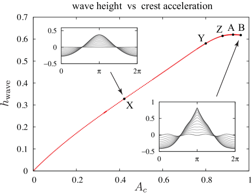
Figure 1. Wave height $h_{\text{wave}}$ versus crest acceleration $A_{c}$ over the range $0\leq A_{c}\leq 0.9639$, along with snapshots of $\eta(x,t)$ for solutions X and B over a quarter-period. For small values of $A_{c}$, the solution is nearly sinusoidal ($\eta\approx-A_{c}\cos x\sin t$, $\varphi\approx-A_{c}\cos x\cos t$, $h_{\text{wave}}\approx A_{c}$). As $A_{c}$ increases, the wave crest sharpens and the surface dynamics become more complicated.

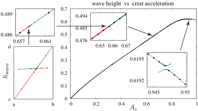
Figure 2. Two “resonant disconnections” in the bifurcation diagram over the range $0<A_{c}<0.9639$ were found in [97]. The first one, with $A_{c}$ between $a=0.658\,621\,068\,280$ and $b=0.658\,621\,070\,350$ and $h_{\text{wave}}$ between $c=0.487\,198\,766\,380$ and $d=0.487\,198\,767\,760$, was only visible when the bifurcation curve was computed in quadruple-precision. The black markers denote points where Floquet multipliers are computed in the present study, while the red, green and gray markers denote the solutions computed in [97] with no stability calculations performed.

Our interest here is in the stability of the solutions at lower amplitude, where the bifurcation curve is either smooth or contains resonant disconnections that are too weak to be observed in numerical simulations to date. In a careful search for such disconnections in quadruple precision, Wilkening and Yu [97] were only able to find two in the range $0\leq A_{c}\leq 0.9639$, namely at $A_{c}=0.658621$ and $A_{c}=0.947$. We note that to see the resonant disconnection at $A_{c}=0.658621$ in Figure 2, we had to zoom in to a window $[a,b]\times[c,d]$ with $\frac{b}{a}-1\approx 3.1\times 10^{-9}$ and $\frac{d}{c}-1\approx 2.8\times 10^{-9}$. Thus, as noted in [97], it is extremely unlikely that this resonance could be computed in double-precision without knowing where to look. Since the effect of such resonances is highly localized and our continuation path jumps over the two disconnections we know about without refining the step length to resolve them, we do not observe any unusual behavior in the dependence of the multipliers on crest acceleration at $A_{c}=0.658621$ or at $A_{c}=0.947$ in Figs. 3–5 below. It is beyond the scope of the present work to quantify the effect of these disconnections on the Floquet multipliers. We emphasize that the stability question is separate from the question of whether solutions occur in smooth families [70, 42]. Given a time-periodic solution, steps (1)–(4) of Algorithm 3.1 will compute its leading Floquet multipliers. Only in the optional step (5) do we assume that nearby parameter values should lead to small changes in the eigenvalues.

Table 1. Parameters used to compute Floquet multipliers of standing water waves.

$$\begin{array}[]{c|c|c|c|c|c|c}\text{$A_{c}$ range}&M&N&n&n^{*}&\text{scheme}&\text{\#}\\ \hline\cr\text{0--0.8871}&768&1440&600&300&5d&297\\ \text{0.8878--0.9295}&1024&1920&600&300&5d&41\\ \text{0.9301--0.9639}&1536&2880&900&300&5d&42\\ 0.8776355\,(Z)&1024&384&800&400&15q&1\\ 0.9263124\,(A)&1536&1200&1000&500&15q&1\\ 0.9620239\,(B)&3840&1152&1500&800&8d&1\end{array}$$

The parameters used to generate the matrices $\hat{E}_{T}$ for this stability study are given in Table 1. The schemes $5d$ and $8d$ in the table correspond to Dormand and Prince’s 5th and 8th order Runge-Kutta methods [35], respectively. (The $d$ stands for double-precision). $15q$ is a 15th order spectral-deferred correction method [49, 71], with computations performed in quadruple-precision. The column labeled ‘#’ gives the number of solutions that were computed in the given range of crest acceleration values. The points are uniformly distributed in each range, except near $A_{c}=0.333$, where additional points were used to resolve a bubble of instability that we observed there. The last 3 entries in the table are re-computations of solutions Z, A, and B on a finer grid to check that the Floquet multipliers do not change when the mesh is refined. For solutions Z and A, these re-computations were done in quadruple precision.

Figures 3–5 show the first 300 Floquet multipliers $\lambda_{j}=|\lambda_{j}|e^{i\sigma_{j}}$ for each of the 380 solutions in the first 3 rows of Table 1. We actually used $n^{*}=360$ for steps (1)–(4) of Algorithm 3.1, which gives 360 eigenvalues sorted by mean wave number. We then re-ordered these using the matching algorithm described in Appendix D to obtain continuous curves depending on the parameter $A_{c}$. Once matched, we kept the first 300, which is sometimes a slightly different set than the 300 eigenvalues of smallest mean wave number. Multipliers not on the unit circle correspond to unstable modes either forward or backward in time. They are plotted with black markers in these figures. Solutions X, Y, Z, A and B are plotted with green markers.

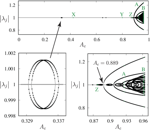
Figure 3. Magnitudes of the first 300 Floquet multipliers of the 380 solutions listed in rows 1–3 of Table 1. We found several bubbles of instability below the first major unstable branch observed by Mercer and Roberts [56] at $A_{c}\approx 0.889$.

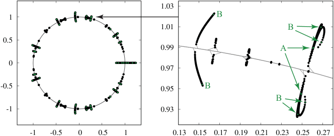
Figure 4. Position in the complex plane of the Floquet multipliers of Fig. 3. Black markers denote multipliers whose distance to the unit circle exceeds $10^{-5}$. All values of $A_{c}$ are plotted simultaneously.

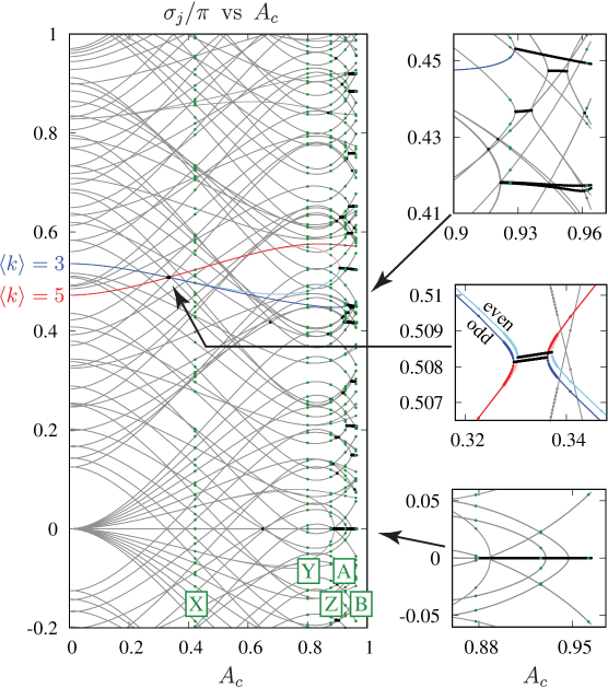
Figure 5. Dependence of the first 300 eigenfrequencies on crest acceleration. Since Floquet multipliers come in conjugate pairs, it was not necessary to plot the entire interval $-1\leq\sigma/\pi\leq 1$. Unstable modes are generated when two eigenfrequencies coalesce and the corresponding multipliers leave the unit circle (see Figs. 3 and 4). These pairs often re-gain stability by joining the unit circle elsewhere, which allows the eigenfrequencies to split apart again.

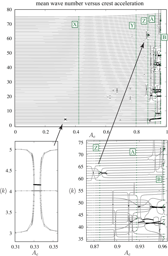
Figure 6. Mean wave number versus crest acceleration for the first 300 Floquet multipliers. The matching algorithm of Appendix D was used to connect the eigenvalues of adjacent problems into continuous curves. Bubbles of instability form when eigenvalues collide and leave the unit circle. Taken together, plots of mean wave number, eigenfrequency (Fig. 5), and magnitude (Fig. 3) give a complete picture of these nucleation events.

Figure 3 shows the magnitude of the Floquet multipliers as a function of $A_{c}$. Mercer and Roberts [56] found that standing waves with crest acceleration below $A_{c}=0.889$ are stable to harmonic perturbation. Our results agree with theirs in that we observe a dominant branch of unstable modes nucleating at $A_{c}=0.889$. However, we also find several smaller bubbles of instability at lower values of $A_{c}$. The first one we observe occurs near $A_{c}=0.333$, which is shown magnified in Figs. 3 and 5. Together with Fig. 6, these figures show that this instability is generated by two nucleation events in which the $\langle k\rangle=3$ and $\langle k\rangle=5$ eigenfrequencies collide, causing two pairs of Floquet multipliers to leave the unit circle. In more detail, at $A_{c}=0$, there are four eigenfunctions of $E_{T}$ with $\langle k\rangle=3$ and four with $\langle k\rangle=5$. The relevant eigenvalues are

$$\lambda_{9}=\overline{\lambda_{10}}=\lambda_{11}=\overline{\lambda_{12}}=e^{-i\pi(2\sqrt{3}-4)}=e^{i\pi(0.535898)},$$

$$\lambda_{17}=\overline{\lambda_{18}}=\lambda_{19}=\overline{\lambda_{20}}=e^{i\pi(2\sqrt{5}-4)}=e^{i\pi(0.472136)}.$$

We choose labels so the corresponding eigenfunctions $\dot{q}_{j}$ are odd for $j\in\{9,10,17,18\}$ and even for $j\in\{11,12,19,20\}$. As $A_{c}$ increases over the range $0\leq A_{c}\leq 0.31$, we see in Figs. 3, 5 and 6 that the eigenfrequencies $\sigma_{9}$ and $\sigma_{11}$ decrease, $\sigma_{17}$ and $\sigma_{19}$ increase, $\langle k\rangle_{9}$ and $\langle k\rangle_{11}$ remain nearly equal to 3, and $\langle k\rangle_{17}$ and $\langle k\rangle_{19}$ remain nearly equal to 5. Conjugate symmetry implies that $\sigma_{10}=-\sigma_{9}$, $\langle k\rangle_{10}=\langle k\rangle_{9}$, etc., but the other pairs that are equal at $A_{c}=0$ (e.g. $\sigma_{9}=\sigma_{11}$ and $\langle k\rangle_{9}=\langle k\rangle_{11}$) split apart slightly once $A_{c}>0$. When $A_{c}$ reaches $0.3295$, $\sigma_{9}$ collides with $\sigma_{17}$ (at $0.50813\pi$), and $\langle k\rangle_{9}$ collides with $\langle k\rangle_{17}$ (at 4.1645). This causes the first pair of Floquet multipliers (with odd eigenfunctions) to leave the unit circle. Shortly after this, at $A_{c}=0.3303$, $\sigma_{11}$ collides with $\sigma_{19}$ (at $0.50826\pi$), and $\langle k\rangle_{11}$ collides with $\langle k\rangle_{19}$ (at 4.1645). This causes the second pair of Floquet multipliers (with even eigenfunctions) to leave the unit circle. The first pair of multipliers rejoins the unit circle at $A_{c}=0.3362$, $\sigma_{9}=\sigma_{17}=0.50826\pi$, $\langle k\rangle_{9}=\langle k\rangle_{17}=4.1569$, and the second pair rejoins at $A_{c}=0.3372$, $\sigma_{11}=\sigma_{19}=0.50841\pi$, $\langle k\rangle_{11}=\langle k\rangle_{19}=4.1568$, restoring stability to the standing waves. The mean wave numbers return to approximately 3 and 5 once $A_{c}$ increases past 0.35 (see Fig. 6).

The above scenario repeats itself for a number of different eigenfrequency collisions between $0<A_{c}<0.889$. However, the widths of the intervals of $A_{c}$ over which the solutions are unstable are quite small, so most standing waves in the range $0<A_{c}<0.889$ appear to be stable. (Mercer and Roberts [56] did not happen to land on any of these windows of instability.) In this parameter regime, the mean wave number of each branch of Floquet multipliers remains close to its initial integer value, except in regions of instability, where the mean wave numbers of two branches briefly coalesce while their eigenvalues lie outside the unit circle (see Fig. 6).

For larger values of crest acceleration ($A_{c}>0.889$), the situation changes. A number of nucleation events occur in which a Floquet multiplier and its complex conjugate collide at $\lambda=1$ and split off along the real axis. This leads to two new eigenvalues outside the unit circle ($\{\lambda,\lambda^{-1}\}\subset\mathbb{R}$). By contrast, for smaller values of $A_{c}$, four eigenvalues leave the unit circle together ($\{\lambda,\overline{\lambda},\lambda^{-1},\overline{\lambda^{-1}}\}\subset\mathbb{C}$). Rather than quickly returning to the unit circle to regain stability, the magnitudes of many of the unstable eigenvalues that nucleate with $A_{c}>0.889$ continue to grow as crest acceleration increases (see Fig 3). In addition, many more bubbles of instability appear and disappear, with multiple nucleation events occurring in rapid succession. In summary, all standing waves with $A_{c}>0.889$ appear to be unstable, with both the number of unstable modes and the magnitude of the largest multiplier growing as $A_{c}$ increases.

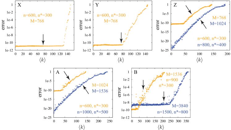
Figure 7. Plots of the residual error of an eigenvector versus its mean wave number for five standing wave solutions in deep water. Arrows point to mode $n^{*}$, the last one used in the Floquet analysis of Section 3. A second calculation was done on a finer grid for solutions Z, A, B to confirm accuracy. These were done in quadruple precision for Z and A, which is why the blue curves do not flatten out due to roundoff errors for small $\langle k\rangle$ in these two cases.

Next we check the accuracy of these Floquet multipliers. Fig. 7 shows the residual error, defined in (3.18), versus the mean wave number $\langle k\rangle$, for solutions X, Y, Z, A, B above. This residual error is made up of two parts: roundoff error, which prevents $J_{1:n,1:n}z=\lambda z$ from holding exactly, and truncation error, which arises when eigenvectors of $J_{1:n,1:n}$ fail to belong to $\ker(J_{n+1:\infty,1:n})$ exactly. Roundoff error is further broken up into errors that occur while solving the PDE to compute the matrix entries of $\hat{E}_{T}$, and errors that occur in the numerical linear algebra routines while diagonalizing $\hat{E}_{T}$. By posing the problem as an overdetermined shooting method and monitoring the decay of Fourier modes [97], we can ensure that $\Delta t$ and $\Delta x$ are small enough that truncation error in time-stepping is smaller than roundoff errors.

The orange markers in Fig. 7 were computed with the same parameters as the other solutions in Figs. 3–5, given in the first three rows of Table 1. The blue markers were computed with the parameters in the remaining three rows of Table 1. For small values of $\langle k\rangle$, roundoff error dominates truncation error in these computations, leading to a flat region at the beginning of each error plot. The two exceptions are the recomputation of solutions Z and A in quadruple precision, where the time-periodic solution was computed to roundoff-error accuracy [97], but $M$ and $n$ were not quite large enough to reach roundoff error in the stability study. We also see in these plots that increasing $M$ and $n$ causes the truncation part of the residual error to shift downward, but can increase the effect of roundoff error as more floating point operations are involved.

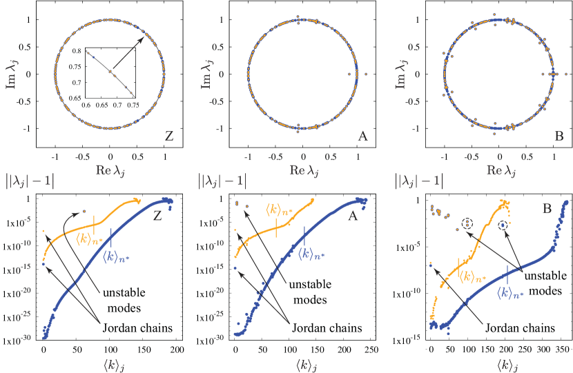
Figure 8. Plots of the first $n^{*}$ Floquet multipliers in the complex plane for solutions Z, A and B (top row) along with deviation of the first $n$ Floquet multipliers from the unit circle (bottom row). This data is the same as in Fig. 7, with blue markers corresponding to the second calculation on a finer grid. The dashed circles contain unstable eigenvalues that were missed on the coarse grid.

In the top row of Fig. 8, we compare the first $n^{*}$ Floquet multipliers of solutions Z, A, B on the original mesh (orange markers, $n^{*}=300$) to the refined mesh (blue markers, $n^{*}=400$, $500$, $800$). Each of the blue markers whose deviation from the unit circle is visible at this resolution has an orange marker directly on top of it, indicating that the original computations are accurate enough to capture the most unstable modes. In the bottom row of Fig. 8, we plot the deviation of all $n$ computed eigenvalues from the unit circle versus the mean wave number of the eigenvalue. For the 6 solutions shown (Z coarse, Z, fine, A coarse, A fine, B coarse, B fine), we have $n=600,800,600,1000,900,1500$, respectively; see Table 1 above. A vertical line is drawn on each curve at the cutoff $\langle k\rangle_{j}$ with $j=n^{*}$, which separates the leading eigenvalues from the discarded eigenvalues. For solution B, we see there are two additional clusters of unstable modes (inside the dashed circles) that were not among the first 300 Floquet multipliers. The first cluster was computed accurately on the coarse mesh but was discarded due to $n^{*}$ being too small, and the second cluster was not resolved on the coarse mesh but emerged on the finer mesh. These modes are stable enough that their deviation from the unit circle in the upper right plot in Fig. 8 is not visible. They can be seen in the bottom right plot due to the logarithmic scale.

The markers labeled “Jordan chains” correspond to the eigenvalue $\lambda=1$, which has algebraic multiplicity 4 but geometric multiplicity 2 in the generic case. As explained in Section 4.2 below, there are two linearly independent Jordan chains associated with $\lambda=1$, each of length 2. This causes errors of order $O(\epsilon^{1/2})$ when $\lambda=1$ splits into two pairs of nearly reciprocal eigenvalues in floating-point arithmetic, where $\epsilon=2.2\times 10^{-16}$ in double precision and $\epsilon=4.8\times 10^{-32}$ in quadruple precision [92]. Each reciprocal pair of eigenvalues can split along the real axis or onto the unit circle as a conjugate pair. If either pair splits along the real axis, the error appears as a spurious unstable mode that deviates from the unit circle by roughly $10^{-7}$ in double-precision or $10^{-14}$ in quadruple-precision. We note that clusters of two or four Floquet multipliers of the form $\{\lambda,\lambda^{-1}\}$ or $\{\lambda,\lambda^{-1},\bar{\lambda},\bar{\lambda}^{-1}\}$ appear as a single point in the bottom plots of Fig. 8 since conjugation does not affect the distance to the unit circle, and if $|\lambda|=1-\delta$ with $\delta$ small, then $|\lambda^{-1}|=1+\delta+O(\delta^{2})$; thus, $\big{|}|\lambda|-1\big{|}=|\delta|\approx\big{|}|\lambda^{-1}|-1\big{|}$.

4.2. Jordan chains associated with $\lambda=1$

The monodromy operator $E_{T}$ possesses at least two Floquet multipliers equal to 1 since the water wave equations are invariant under translation in time and space. Indeed, if $q=(\eta,\varphi)$ is a time-periodic solution of $\partial_{t}q=F(q)$, then

$$p_{0}(x,t)=\partial_{t}q(x,t)\qquad\text{and}\qquad p_{1}(x,t)=\partial_{x}q(x,t)$$ (4.1)

satisfy the linearized equation $\partial_{t}p=DF(q(t))p$ as well as $p(x,T)=p(x,0)$. Thus,

$$E_{T}[p_{j}(\cdot,0)]=\lambda p_{j}(\cdot,0),\qquad\lambda=1,\;\;j=0,1.$$ (4.2)

For symmetric standing waves, $\eta$ and $\varphi$ are even functions of $x$ for all $t$, so $p_{0}(x,0)$ is even while $p_{1}(x,0)$ is odd.

There are three ways to compute the eigenfunctions $p_{0}(x,0)$ and $p_{1}(x,0)$. We can differentiate the nonlinear solution $q$ with respect to $t$ and $x$, respectively, as in (4.1). We can compute all the eigenvalues and eigenfunctions of a numerical approximation of $E_{T}$, splitting them into even and odd eigenfunctions, as was done in Figures 3–8 above. Extracting the $\lambda=1$ eigenfunctions leads to two copies of $p_{0}(x,0)$ and two copies of $p_{1}(x,0)$, up to constant factors. (Jordan chains are responsible for the duplicate eigenvectors, which cause the eigenvector matrix to be singular.) Or we can compute the kernel of $E_{T}-I$. This last approach has the advantage that with minor modification, we can obtain Jordan chain information as well. Using the algorithm of Wilkening [92], we have found that $p_{0}(x,0)$ and $p_{1}(x,0)$ generally have an associated vector $p_{j}^{(1)}(x,0)$ such that

$$E_{T}[p_{j}^{(1)}(\cdot,0)]=p_{j}(\cdot,0)+\lambda p_{j}^{(1)}(\cdot,0),\qquad\lambda=1.$$ (4.3)

These associated vectors have a natural physical interpretation. For example, if we think of the period as a bifurcation parameter controlling $q(x,t;T)$, then time-periodicity gives $q(x,T;T)=q(x,0;T)$. Thus, $\partial_{t}q(x,T;T)+\partial_{T}q(x,T;T)=\partial_{T}q(x,0;T)$. It follows that

$$p_{0}^{(1)}(x,t)=-\partial_{T}q(x,t;T)$$ (4.4)

is a solution of the linearized equation and satisfies

$$E_{T}[p_{0}^{(1)}(\cdot,0)]=p_{0}^{(1)}(\cdot,T)=p_{0}(\cdot,0)+p_{0}^{(1)}(\cdot,0),$$ (4.5)

as required. Iterating this equation gives

$$E_{T}^{m}[p_{0}^{(1)}(\cdot,0)]=mp_{0}(\cdot,0)+p_{0}^{(1)}(\cdot,0),\qquad(m\in\mathbb{Z}),$$ (4.6)

which can be interpreted as expressing

$$q(x,mT;T-\varepsilon) \approx q(x,m(T-\varepsilon);T-\varepsilon)+\varepsilon mq_{t}(x,m(T-\varepsilon);T-\varepsilon)$$ (4.7)

$$=q(x,0;T-\varepsilon)+\varepsilon mq_{t}(x,0;T-\varepsilon)$$

$$\approx q(x,0;T)+\varepsilon[mq_{t}(x,0;T)-q_{T}(x,0;T)],\qquad(m\in\mathbb{Z}).$$

The idea here is that if the initial condition is perturbed in the direction of another standing wave with a slightly shorter period, then each time $t$ advances by the period $T$ of the original solution, it will travel slightly further in the $q_{t}(\cdot,0)$ direction. We note that these Jordan chains lead to “secular instabilities” in the solution that grow linearly in time. We will still consider a solution to be stable if these are the only instabilities.

This argument that Jordan chains of the form (4.4) should exist assumes that standing waves occur in smooth families. Even if this is not the case, e.g. if there are infinitely many disconnections of the type shown in Figure 2 on scales too small to be observed in quadruple-precision arithmetic, the monodromy operator may still have Jordan chains. In our numerical experiments, these Jordan chains are always present, except at turning points, where they become genuine eigenvectors. For example, $T$ reaches a relative maximum of $T=6.543\,698$ at $A_{c}=0.889\,283$. Near such a turning point, it is better to use a different coefficient $c_{k}$ in (2.11) than $c_{0}=T$ as the bifurcation parameter; we used $c_{5}$. From $q(x,T;c_{k})=q(x,0;c_{k})$ we have

$$\frac{\partial T}{\partial c_{k}}\frac{\partial q}{\partial t}(x,T;c_{k})+\frac{\partial q}{\partial c_{k}}(x,T;c_{k})=\frac{\partial q}{\partial c_{k}}(x,0;c_{k}).$$ (4.8)

Thus, rescaling the associated vector via $p_{0}^{(1)}(x,t)=-(\partial q/\partial c_{k})(x,t;c_{k})$, the first term on the right-hand side of (4.3) acquires a factor of $\partial T/\partial c_{k}$ that vanishes at a turning point. As a result, $p_{0}^{(1)}(x,t)$ becomes an independent eigenvector rather than blowing up like $\partial q/\partial T$ does. Similarly, using $c_{1}$ to parametrize the bifurcation from the zero-amplitude wave, we have $\partial T/\partial{c_{1}}=0$, which explains why Jordan chains did not arise in Section 3.3.

We expected to find the associated vector $p_{0}^{(1)}(\cdot,0)$ when we computed Jordan chains at $\lambda=1$ using the numerical algorithm of [92], but we did not anticipate finding the second associated vector $p_{1}^{(1)}(\cdot,0)$. Just as perturbation in the direction of $p_{0}^{(1)}(\cdot,0)$ leads to linear drift in time over multiple cycles due to a slight change in period, perturbation in the $p_{1}^{(1)}(\cdot,0)$ direction should lead to linear drift in space. This suggests the existence of traveling-standing waves bifurcating from the pure standing wave solutions. We have investigated this, and have successfully computed a two-parameter family of traveling-standing waves, which will be reported on elsewhere [96].

4.3. Counter-propagating solitary waves in shallow water

Wilkening and Yu [97] found that varying the fluid depth of standing water waves leads to nucleation or vanishing of loop structures in the bifurcation curves that meet or nearly meet at perfect or imperfect bifurcations. Closed loops can even nucleate in isolation and later join with pre-existing families of solutions. Disconnections and bifurcations tend to disappear as the fluid depth increases, though some persist in the infinte depth limit, as seen above in Fig. 2. These disconnections and gaps in the bifurcation curves can be interpreted [97] as numerical manifestations of the Cantor-like structures that arise in analytical studies of standing water waves due to small divisors [70, 42]. In shallow water, resonances abound, and the bifurcation curves are highly fragmented even in double-precision. This is illustrated in the left panel of Fig. 9, which shows wave height versus period for symmetric standing waves of wavelength $2\pi$ in a fluid of depth $h=0.05$. Here wave height is defined as the crest to trough height at $t=T/4$, when the fluid comes to rest. This differs by a factor of two from the convention used in Section 4.1 above. These solutions were first computed in [97], where a different set of bifurcation curves are given that show how $\hat{\varphi}_{k}(0)$ varies with $T$ for $k=1$, 17 and 36. The periods of these waves are much longer than their infinite depth counterparts. For example, in the linear regime, $T=2\pi/\sqrt{gK\tanh Kh}=28.1$ when $h=0.05$ and $T=6.28$ when $h=\infty$. In both cases, $g=1$ and $K=1$.

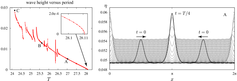
Figure 9. Wave height versus period for a family of standing waves in shallow water ($h=0.05$) and time-elapsed snapshots of solution A over a period. (left) Many more disconnections are visible at this depth than were observed in the infinite-depth case above. (right) The arrows show the initial direction of motion at $t=0$. The waves return to this initial position at $t=T/2$, but moving in the opposite direction. Small vertical oscillations are visible in the wave troughs and crest trajectories as the waves travel back and forth between collisions.

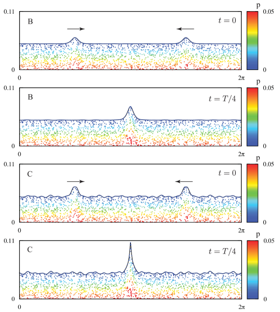
Figure 10. Solutions B and C from Figure 9 at times $t=0$ and $t=T/4$. Solution B remains calm between collisions while solution C is choppy. These images are taken from movies in which passively advected particles have been added to the fluid for visualization, color coded by pressure.

Beyond the linear regime, standing waves in shallow water take the form of counter-propagating solitary waves that repeatedly collide with one another. These waves are special in the sense that low-amplitude, high-frequency oscillatory modes are present initially and have been tuned so that no new radiation is generated each time the solitary waves collide. The right panel of Fig. 9 shows time-elapsed snapshots of solution A in the bifurcation diagram in the left panel, and Fig. 10 shows solutions B and C at $t=0$ and $t=T/4$. Figure 10 also shows the pressure beneath the waves and marker particles for visualizing the flow in movies of these simulations. Aside from the solitary waves, solution B remains calm throughout its evolution. By contrast, the solitary waves of solution C travel over a choppy and erratic background of higher-frequency waves that are clearly visible in static images.

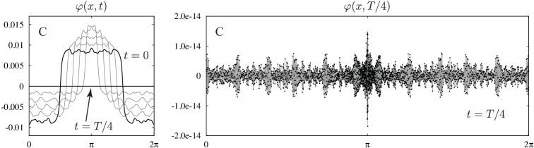
Figure 11. Evolution of the velocity potential of solution C over a quarter period. (left) The velocity potential jumps rapidly at the location of the solitary waves, where fluid velocity $\mathbf{u}=\nabla\phi$ is highest. (right) At $t=T/4$, the velocity potential has been driven to zero (up to roundoff error), yielding a minimum value of $f=3.3\times 10^{-30}$ for the objective function in (2.13). For mesh refinement, we set $\nu=2$, $\theta_{1}=0.85$, $\theta_{2}=0.15$, $\kappa_{1}=0$, $\kappa_{2}=2$, $\rho_{2}=0.15$, $M_{1}=2048$, $N_{1}=204$, $M_{2}=3072$ and $N_{2}=108$. The computation took 43 minutes using an NVIDIA Tesla M2050 GPU, with 32 minutes devoted to computing the Jacobian.

The height of the solitary waves relative to the fluid depth is remarkable for both of these solutions. For solution C, when the solitary waves collide and the fluid comes to rest, the wave crest reaches a height of $0.10636$ (measured from the bottom), which is more than twice the fluid depth $h=0.05$. It is surprising that such a jet could form and then return back along its path to form a time-periodic solution. Figure 11 shows snapshots of $\varphi(x,t)$ for solution C and a plot of the residual error at $t=T/4$, confirming that the wave actually comes to rest at this time. Because the wave amplitudes of these solutions are so large, it is not appropriate to consider $\eta(x,t)$ as a small perturbation of a flat wave profile, to ignore vertical components of velocity, nor to assume hydrostatic pressure forces. Thus, most of the assumptions one makes in deriving model equations such as Serre’s equations, the Boussinesq system, or the Korteweg de-Vries equation, break down [89]. These wave interactions are fully (as opposed to weakly) nonlinear. Nevertheless, solutions such as B have many properties in common with the perfectly elastic collisions of solitons that occur in integrable equations.

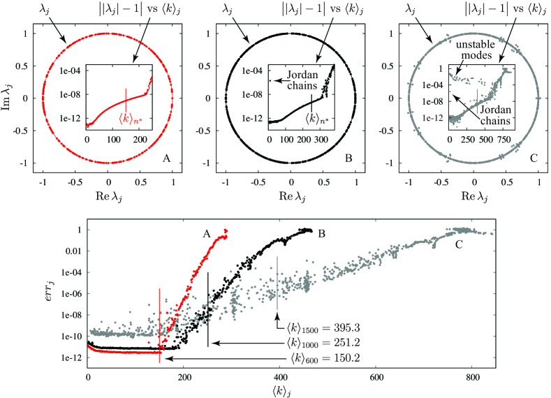
Figure 12. Floquet stability analysis of solutions A–C in Figures 9–11. (top row) The first $n^{*}=600$, $1000$ and $1500$ Floquet multipliers $\lambda_{j}$ are plotted in the complex plane. The inset graphs show that the more reliable eigenvalues (of lower mean wave number) satisfy $|\lambda_{j}|=1$ with high accuracy, except for the unstable modes of solution C and the eigenvalue $\lambda=1$, which has Jordan chains that cause it to split. (bottom) Residual error versus mean wave number. The vertical lines give the cutoff $\langle k\rangle_{n^{*}}$ beyond which the eigenvalues were discarded.

Next we consider the stability of these solutions with respect to harmonic perturbations. The results are summarized in Figure 12. For solutions A and B, we used uniform spatial grids with $M^{(A)}=1536$ and $M^{(B)}=2048$ gridpoints. For solution C, we used mesh refinement near $(x,t)=(\pi,T/4)$ and $(x,t)=(0,3T/4)$. More specifically, in the notation of Section 2.1, we set $\nu=5$, $\kappa_{l}=\{0,2,0,-2,0\}$, $\theta_{l}=\{0.21,0.08,0.42,0.08,0.21\}$, and $M^{(C)}_{l}=\{3888$, $5184$, $3888$, $5184$, $3888\}$. For solutions $\{A,B,C\}$, we computed $n=\{1200$, $2000$, $4000\}$ Floquet multipliers, kept the first $n^{*}=\{600,1000,1500\}$ ordered by mean wave number, and discarded the rest. All the multipliers of solutions A and B lie on the unit circle, with $\big{|}|\lambda_{j}|-1\big{|}$ ranging from $10^{-13}$ for low values of $\langle k\rangle$ to $10^{-9}$ for large values of $\langle k\rangle$, up to the cutoff point $\langle k\rangle_{n^{*}}$. As in the infinite depth case, a pair of Jordan chains of length 2 is associated with the two-dimensional eigenspace at $\lambda=1$. Numerically, this degenerate eigenvalue splits into a cluster of four simple eigenvalues with errors on the order of $\sqrt{\epsilon}$, where $\epsilon$ is machine precision [30]. These four eigenvalues consist of two pairs of nearly reciprocal eigenvalues, i.e. the product of the eigenvalues in each pair differs from 1 by $O(\epsilon)$. For solution A, the degenerate eigenvalue happens to split into two complex conjugate pairs that lie on the unit circle (since $\lambda^{-1}=\bar{\lambda}+O(\epsilon)$); thus, they do not appear anomalous in the plot of $\big{|}|\lambda_{j}|-1\big{|}$. For solution B, the degenerate eigenvalue split into two pairs of real eigenvalues; and for solution C, the degenerate eigenvalue split into one pair of real eigenvalues and one pair of complex conjugate eigenvalues. Regardless of how they split, which is unpredictable due to roundoff errors, these Jordan chains correspond to nearby families of time-periodic solutions and traveling-standing waves. Thus, solutions A and B appear to be linearly stable to harmonic perturbation (aside from the secular instabilities of the Jordan chains). In numerical experiments that will be reported elsewhere [95], we find that nearby initial conditions evolved under the nonlinear equations of motion remain close to these stable time-periodic solutions over thousands of cycles.

By contrast, solution C has many eigenvalues $\lambda_{j}$ outside the unit circle. Perturbation of the time-periodic solution in these directions will lead to exponential growth. The growth is actually quite slow, with the largest multiplier being $\rho=|\lambda_{\text{max}}|=1.062$. This is the amplification factor over a cycle (consisting of two collisions of the solitary waves), not the growth rate per unit time. Thus, if roundoff error contributes an error of $10^{-13}$ per cycle, the accumulated error after $p$ cycles is expected to be around $10^{-13}\rho(\rho^{p}-1)/(\rho-1)$. This is roughly what happens in a long-time simulation, except there is a large startup phase of about 100 cycles where the solution remains time-periodic to 13 digits. The next 380 cycles look time-periodic to the eye, but exhibit exponential growth when $\|\eta(\cdot,T)-\eta(\cdot,0)\|$ is computed. Over the next 90 cycles, the solitary waves fall out of phase with each other and the background radiation grows in amplitude. Finally, after evolving solution C through 571 cycles, the numerical solution blows up, with GMRES failing to converge when solving for the dipole density $\mu$.

4.4. Gravity-capillary solitary wave interactions in deep water

We now investigate the effect of surface tension on the dynamics and stability of time-periodic water waves. For simplicity, we consider only the infinite depth case. Concus [20] and Vanden-Broeck [87] computed the leading terms in a perturbation expansion for standing water waves with surface tension, building on the work of Penney and Price [68] and Tadjbakhsh and Keller [82]. Concus predicted that the quadratic correction to the period in the infinte depth case is

$$T=\frac{2\pi}{\sqrt{1+\gamma}}\left(1+\frac{8-27\delta-36\delta^{2}-81\delta^{3}}{32(1-9\delta^{2})}\epsilon^{2}+O(\epsilon^{4})\right),\qquad\epsilon=c_{1}=\hat{\varphi}_{1}(0),$$ (4.9)

where $\gamma=\frac{\sigma k^{2}}{\rho g}$ is a dimensionless surface tension parameter, $\delta=\frac{\gamma}{1+\gamma}$ is the relative capillarity, and $c_{1}$ refers to the notation of Equation (2.11). Wilkening and Yu [97] computed a family of standing waves of this type using the overdetermined shooting method described in Section 2 and confirmed (4.9) in the special case of $\gamma=1$ and $\delta=1/2$. It was also found in [97] that beyond the linear regime, larger-amplitude standing waves of this type take the form of counter-propagating solitary depression waves that repeatedly collide and reverse direction. We computed the leading Floquet multipliers of a moderate-amplitude wave in this family, namely solution B of Section 4.6 of [97], and found that it is stable to harmonic perturbations. The results are summarized in Figure 13.

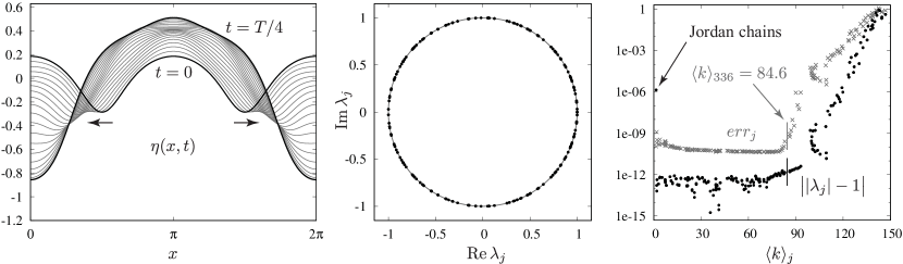
Figure 13. Stability calculation of a moderate-amplitude standing gravity-capillary water wave with crest-to-trough height of 1.3693. (left) At this amplitude, the wave consists of counter-propagating depression waves that repeatedly collide and change direction. (center) The leading $n^{*}=336$ Floquet multipliers lie on the unit circle. (right) Plots of $err_{j}$ and $\big{|}|\lambda_{j}|-1\big{|}$ versus mean wave number. We computed $n=600$ eigenvalues of the monodromy operator on a grid with $M=1024$ gridpoints and $N=28800$ timesteps over a full period. The underlying wave only needs $M=256$ gridpoints and 720 timesteps over a quarter period to drive the objective function $f$ in (2.13) down to $3.7\times 10^{-28}$, but additional timesteps are needed to resolve the dynamics of high-frequency perturbations. Surface tension increases the stiffness of the water wave equations, and requires more timesteps than the $\sigma=0$ case with an explicit method. We did not employ the small scale decomposition strategy of Hou, Lowengrub and Shelley [38].

Next we search for a new type of time-periodic gravity-capillary water wave built from counter-propagating solitary waves of the type discovered by Longuet-Higgins [52] and studied by Vanden Broeck [88] and Milewski et. al. [58]. Our idea is to collide two identical traveling waves of this type (moving in opposite directions) together, see how they interact, and optimize the initial conditions of the combined wave to obtain a time-periodic solution.

The first step is to compute traveling waves. While several methods have been developed previously for this purpose [74, 76, 88, 58, 84], we modified the trust-region code we wrote to compute standing water waves so that it can also compute traveling waves. Details are given in Appendix B. Instead of computing entire families of traveling gravity-capillary waves, we will focus on two solutions, with amplitudes close to the ones plotted in Figure 4 of [58]. Following the conventions of that paper, we temporarily assume $\sigma/\rho=1$ and $g=1$ in (2.1) and try starting guesses of the form

$$\text{Solution A:}\qquad\eta_{0}(x)=-0.15\frac{\cos x-a}{1-a}\operatorname{sech}(x/6.4),\qquad\varphi_{0}=cH\eta_{0},\qquad\left\{\begin{aligned} a&=\operatorname{sech}(3.2\pi),\\ c&=1.408,\end{aligned}\right.$$ (4.10)

$$\text{Solution B:}\qquad\eta_{0}(x)=-0.32\frac{\cos x-a}{1-a}\operatorname{sech}(x/2.4),\qquad\varphi_{0}=cH\eta_{0},\qquad\left\{\begin{aligned} a&=\operatorname{sech}(1.2\pi),\\ c&=1.385.\end{aligned}\right.$$

These functions $\eta_{0}$ have roughly the right oscillation frequencies and decay rates (within 20 percent) as the graphs given in [58]. We have estimated $\varphi$ from the linearized equations (3.13), which imply for a wave traveling at speed $c$ that $-c\eta_{x}=\mathcal{G}\varphi$, or $\varphi=cH\eta$, where $H$ is the Hilbert transform. While linear theory is not an accurate model in this regime, it works well enough as a starting point for the trust region shooting method to converge to a traveling solution of the nonlinear equations. The values of wave speed, $c$, were estimated from the graph in Figure 1 of [58], and the parameter $a$ was chosen so that $\eta_{0}(x)$ has zero mean. The actual values of $c$ for waves of amplitude $-0.15$ and $-0.32$ turned out to be $1.40995$ and $1.38558$, respectively.

In our code, we assume the domain is $[0,2\pi]$; however, the convention that $\sigma/\rho=1$ leads to traveling waves that extend well outside of this range. So instead of choosing $L=(\tilde{\sigma}/\tilde{\rho}\tilde{g})^{1/2}$ and $\tau=(\tilde{\sigma}/\tilde{\rho}\tilde{g}^{3})^{1/4}$ as characteristic length and time scales, with notation as in (2.3), we use $L=40(\tilde{\sigma}/\tilde{\rho}\tilde{g})^{1/2}$ and $\tau=\sqrt{40}(\tilde{\sigma}/\tilde{\rho}\tilde{g}^{3})^{1/4}$. For real water (assuming $\tilde{\sigma}=72\text{ dyne}/\text{cm}$), this is $L=10.8$ cm and $\tau=0.105$ s. In the dimensionless equation (2.1), this causes $\sigma/\rho$ to change from 1 to $0.000625$ and $g$ to remain 1. The starting guesses (4.10) are modified by replacing $x$ by $40x$ on the right-hand-side in the formulas for $\eta_{0}(x)$, dividing $0.15$ and $0.32$ by 40, and dividing $1.408$ and $1.385$ by $\sqrt{40}$. The numerical values of wave height and velocity potential will then decrease by factors of $40^{-1}$ and $40^{-3/2}$, respectively. With starting guess A for the traveling wave, the trust region shooting method reduced $f$ to $3.8\times 10^{-24}$ in only 12 function evaluations and 2 Jacobian calculations (using $M=2048$ gridpoints and $n=901$ unknowns). With starting guess B, 10 function evaluations and 1 Jacobian calculation were sufficient to minimize $f$ to $4.5\times 10^{-26}$, using $M=3072$ gridpoints and $n=1801$ unknowns. The former calculation took 34 seconds while the latter took 111 seconds. In both cases, the amplitude, $\eta(0,0)$, was fixed via (2.14) to be $-0.15/40$ for solution A and $-0.32/40$ for solution B.

Once a traveling wave is found, we obtain a starting guess for counter-propagating time-periodic solutions by defining the initial conditions

$$\eta_{0}(x) =\eta_{0}^{(\text{trav})}(x-\pi/2)+\eta_{0}^{(\text{trav})}(x-3\pi/2),$$ (4.11)

$$\varphi_{0}(x) =\varphi_{0}^{(\text{trav})}(x-\pi/2)-\varphi_{0}^{(\text{trav})}(x-3\pi/2).$$

The sign change in velocity potential causes the second wave to travel left. The Fourier modes of the initial conditions take the form (B.2) for traveling waves and (2.11) for counter-propagating waves. They are related via

$$\hat{\eta}_{k}(0)=2\cos(k\pi/2)\,\hat{\eta}^{(\text{trav})}_{k}(0),\qquad\hat{\varphi}_{k}(0)=-2i\sin(k\pi/2)\,\hat{\eta}^{(\text{trav})}_{k}(0),\qquad(k\in\mathbb{Z}).$$ (4.12)

From this starting guess, we minimized the objective function (2.13) assuming initial conditions of the form (2.11). We specified $\eta(\pi/2,0)$ to be $-0.00375$ for solution A and $-0.008$ for solution B by appending equation (2.14) to the residual vector $r$.

The results are summarized in Figures 14 and 15. In both cases, the wave packets approach each other without changing shape until they start to overlap. As they collide, they produce a localized standing wave that grows in amplitude to the point that $\varphi$ becomes exactly 0 (at time $T/4$). The standing wave then decreases in amplitude and the two traveling waves emerge and depart from one another. As in Section 4.3 above, the background radiation is synchronized with the collision so as not to grow in amplitude. The background radiation is invisible to the eye in solution A, and takes the form of small-amplitude, non-localized, counter-propagating waves in solution B when viewed as a movie at closer range than shown in Figure 15. A Floquet stability analysis summarized in Figures 14 and 15 shows that solution A is linearly stable to harmonic perturbations while solution B is unstable.

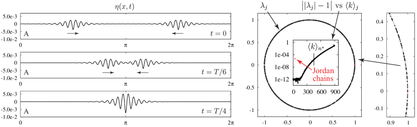
Figure 14. Counter-propagating gravity-capillary waves with $\sigma/\rho=0.000625$ and initial amplitude $\eta(\pi/2,0)=\eta(3\pi/2,0)=-0.00375$. At time $t=T/4$, the velocity potential is zero and the fluid comes to rest. The period is $T=28.206$. We used $M=2048$ grid points and $n=620$ initial unknown Fourier modes to minimize $f$ to $2.41\times 10^{-30}$ with only 8 function evaluations and 3 Jacobian calculations. (right) The first $n^{*}=1800$ Floquet multipliers all lie on the unit circle, indicating that this solution is linearly stable to harmonic perturbations. We computed $n=3600$ columns of $\hat{E}_{T}$ with $M=3600$ gridpoints and $N=2700$ timesteps. The calculation took 5 days. As in Section 4.3, the eigenvalue $\lambda=1$ has two linearly independent Jordan chains of length two that cause the eigenvalue to split in the numerical calculation of Floquet multipliers.

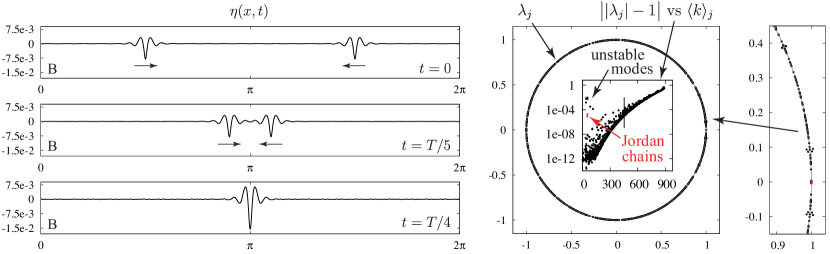
Figure 15. Counter-propagating gravity-capillary waves with $\sigma/\rho=0.000625$ and initial amplitude $\eta(\pi/2,0)=\eta(3\pi/2,0)=-0.008$. We used $M=3072$ gridpoints and $n=900$ unknown Fourier modes of the initial condition to obtain $f=3.9\times 10^{-28}$. The period of this solution is $T=28.711$. (right) Some of the first 1800 Floquet multipliers lie outside the unit circle, indicating that this solution is linearly unstable.

5. Conclusion

We have developed an efficient algorithm for computing the stability spectra of standing water waves in finite and infinite depth, with and without surface tension. The method involves two levels of truncation. First, a truncated version of the monodromy operator is computed in Fourier space by considering perturbations of the initial condition up to a given wave number. This decouples the size of the truncated operator from the size of the mesh, allowing all the matrix entries to be computed accurately. Otherwise our method is similar to that of Mercer and Roberts [56], who also solve the linearized Euler equations about the time-periodic solution with multiple initial conditions in order to study stability. We then introduce a “mean wave number” to order the eigenvalues of the truncated operator. This ordering has the effect of moving accurately computed eigenvalues to the front, as seen in plots of the residual error (3.18) obtained by substituting an eigenpair of the truncated operator into the full state transition matrix after zero-padding the eigenvector. We retain a specified number of Floquet multipliers (ordered in this way) and discard the rest, which is the second truncation step. Finally, we define a linear assignment problem to match eigenvalues of nearby standing waves in order to track individual eigenvalues from the zero-amplitude wave to large-amplitude waves via homotopy. This reveals, for example, which modes are involved when bubbles of instability nucleate.

In addition to studying the stability of classical standing waves in deep water, we explore the stability of new or recently discovered families of time-periodic water waves that involve counter-propagating solitary wave collisions, e.g. of gravity waves in shallow water and capillary-gravity waves in deep water. The examples in Figures 12AB, 13 and 14 show that large-amplitude water waves of various types can be stable to harmonic perturbations both forward and backward in time. Computing these waves in the first place is a significant challenge. One novelty of the gravity-capillary waves computed in Figures 14 and 15 is that we searched directly for large-amplitude time-periodic solutions without using numerical continuation to get there. This suggests an abundance of different types of time-periodic water waves and also speaks to the robustness of the shooting method to solve two-point boundary value problems with fairly inaccurate starting guesses. False positives are avoided by resolving the solutions with spectral accuracy and formulating the problem as an overdetermined minimization problem. In previous work [94], the author has faced similar challenges in computing relative-periodic elastic collisions of co-propagating solitary water waves that resemble cnoidal solutions of KdV.

Many of the numerical results of Section 4 call for future work. For example, what is the physical mechanism responsible for the bubbles of instability we discovered with crest acceleration far below the stability threshold $A_{c}=0.889$? In a follow-up paper [95], we will show that perturbing the solution of the nonlinear equations near one of these bubbles of instability leads to a cyclic pattern in which the perturbation grows for thousands of cycles and then, surprisingly, decays for thousands of cycles to return close to the standing wave in a nearly time-reversed fashion to its initial excursion. This sequence repeats with some variation in how close the wave returns to the standing wave before latching onto another growing mode. Bryant and Stiassnie [12] observed similar recurrent behavior from sideband instabilities on a domain containing 9 replicas of the standing wave, so this type of recurrent pattern may be a common mechanism associated with a single pair of unstable Floquet multipliers $\lambda$ and $\bar{\lambda}$.

Another natural question is the extent to which linear stability predicts the long-time dynamics of perturbations of the nonlinear equations. It has been observed in the literature [15, 55, 81, 22, 23, 58] that although solitary water wave collisions are inelastic, the residual radiation of such a collision can be remarkably small. In [95], we will show that if two identical counter-propagating traveling water waves (i.e. Stokes waves) of a certain amplitude are combined at $t=0$ via (4.11), the solution remains close to solution B of Figures 9–12 for all 5000 cycles we computed. The first several collisions of the Stokes waves produce radiation that becomes visible in the wave troughs after a few cycles; however, it quickly saturates and does not grow beyond the size of the background oscillations present in Solution B, which we found to be linearly stable to harmonic perturbations. The amplitude of the component traveling waves of the initial condition (4.11) was chosen to eliminate temporal drift relative to solution B. This drift is caused by the secular instability of one of the Jordan chains of length two associated with $\lambda=1$. The secular instability of the other Jordan chain was eliminated by even symmetry of the initial condition.

We were initially puzzled by this second Jordan chain. As explained in Section 4.2, one of these chains corresponds to the change in period when the amplitude of the standing wave is increased. Equation (4.7) shows that a perturbation in this direction will cause the wave to drift forward or backward in time relative to the underlying standing wave. We eventually realized that the other Jordan chain corresponds to a perturbation direction in which the wave drifts left or right in space as it evolves through successive cycles. This suggests a bifurcation direction in which the standing wave begins to travel as it oscillates. The only reference to such waves we have seen in the literature is a parenthetical comment by Iooss, Plotnikov and Toland [42]: “it is possible to imagine more general solutions, for example, ‘travelling-standing-wave’ solutions, of the free boundary problem.” Using the Jordan chains as a guide, we have successfully computed a two-parameter family of traveling-standing waves that return to a spatial translation of themselves at periodic time-intervals. Pure traveling waves and standing waves are special cases that occur at certain values of the second bifurcation parameter. These will be reported on elsewhere [96].

We have focused on harmonic stability in this paper, which is natural for standing waves evolving in a rigid container. In future work [96], we will generalize the method to investigate stability with respect to subharmonic perturbations in the more general context of traveling-standing waves. Mercer and Roberts [56] considered subharmonic perturbations by replicating the underlying standing wave and looking at harmonic stability over a larger spatial period. Instead, we will consider quasi-periodic perturbations of the linearized equations, similar to what has been done recently for traveling waves [8, 7, 50, 51, 27, 54, 43, 61, 29, 84]. There are many technical challenges for the traveling-standing problem that do not arise in the pure traveling case.

Subharmonic stability involves solving the linearized Euler equations with quasi-periodic perturbations. A natural next step is to seek fully nonlinear quasi-periodic solutions of the free-surface Euler equations (2.1). The relative-periodic solutions computed in [94] and the traveling-standing waves computed in [96] are examples of waves with two quasi-periods. A recent paper of Berti and Montalto [10] proves existence of gravity-capillary water waves with more than two quasi-periods using Nash-Moser theory. We hope to extend the overdetermined shooting method to compute such waves with or without surface tension and study their properties. Spatially quasi-periodic traveling waves and other generalizations also appear to be within reach with the tools we are developing.

Appendix A Boundary integral formulation

In this section, we briefly describe how we compute the Dirichlet-Neumann operator in (2.5). Further details (with derivations) may be found in Wilkening and Yu [97]. The signs in (A.4) below correct a typo in [97], where $K_{1}+K_{2}$ and $G_{1}+G_{2}$ were written in several equations without changing the sign in the formulas for $K_{2}$ and $G_{2}$. The derivations in [97] are otherwise correct.

To compute $\mathcal{G}\varphi$, we solve the integral equation

$$\frac{1}{2}\mu(\alpha)+\frac{1}{2\pi}\int_{0}^{2\pi}K(\alpha,\beta)\mu(\beta)\,d\beta=\varphi(\xi(\alpha))$$ (A.1)

for the dipole density $\mu(\alpha)$, and then compute

$$\mathcal{G}\varphi(\xi(\alpha))=\frac{1}{|\xi^{\prime}(\alpha)|}\left[\frac{1}{2}H\gamma(\alpha)+\frac{1}{2\pi}\int_{0}^{2\pi}G(\alpha,\beta)\gamma(\beta)\,d\beta\right],$$ (A.2)

where $\gamma(\alpha)=\mu^{\prime}(\alpha)$ is the vortex sheet strength, $H$ is the Hilbert transform (with symbol $\hat{H}_{k}=-i\operatorname{sgn}(k)$), and

$$x=\xi(\alpha)$$ (A.3)

is a monotonic parametrization of the interval $[0,2\pi]$. Normally $\xi(\alpha)=\alpha$, but other choices are useful for refining the mesh in regions of high curvature [97]. In these formulas,

$$K(\alpha,\beta) =K_{1}(\alpha,\beta)-K_{2}(\alpha,\beta),$$ (A.4)

$$G(\alpha,\beta) =G_{1}(\alpha,\beta)-G_{2}(\alpha,\beta),$$

where

$$K_{1} =\operatorname{Im}\left\{\frac{\zeta^{\prime}(\beta)}{2}\cot\frac{\zeta(\alpha)-\zeta(\beta)}{2}-\frac{1}{2}\cot\frac{\alpha-\beta}{2}\right\}, \quad K_{2} =\operatorname{Im}\left\{\frac{\bar{\zeta}^{\prime}(\beta)}{2}\cot\frac{\zeta(\alpha)-\bar{\zeta}(\beta)}{2}\right\},$$

$$G_{1} =\operatorname{Re}\left\{\frac{\zeta^{\prime}(\alpha)}{2}\cot\frac{\zeta(\alpha)-\zeta(\beta)}{2}-\frac{1}{2}\cot\frac{\alpha-\beta}{2}\right\}, \quad G_{2} =\operatorname{Re}\left\{\frac{\zeta^{\prime}(\alpha)}{2}\cot\frac{\zeta(\alpha)-\bar{\zeta}(\beta)}{2}\right\}.$$

Here $\mathbb{R}^{2}$ has been identified with $\mathbb{C}$ and the free surface is parametrized by

$$\zeta(\alpha)=\xi(\alpha)+i\eta(\xi(\alpha)).$$ (A.5)

When the fluid depth is infinite, $K_{2}$ and $G_{2}$ are dropped; otherwise, the bottom boundary is assumed to be at $y=0$ so that $\bar{\zeta}$ is the mirror image of the free surface. When $\beta=\alpha$, we set

$$K_{1}(\alpha,\alpha) =-\operatorname{Im}\{\zeta^{\prime\prime}(\alpha)/[2\zeta^{\prime}(\alpha)]\},$$ (A.6)

$$G_{1}(\alpha,\alpha) =\phantom{-}\operatorname{Re}\{\zeta^{\prime\prime}(\alpha)/[2\zeta^{\prime}(\alpha)]\},$$ (A.7)

which makes them continuous functions.

The integrals in (A.1) and (A.2) are approximated with spectral accuracy via the trapezoidal rule with uniformly spaced collocation points $\alpha_{j}=2\pi j/M$, $0\leq j<M$. The matrix entries $K_{ij}=K(\alpha_{i},\alpha_{j})$ and $G_{ij}=G(\alpha_{i},\alpha_{j})$ are computed in parallel on a GPU, which involves $O(M)$ communication costs for $O(M^{2})$ work. This makes evaluation of $\phi_{x}$ and $\phi_{y}$ in (2.1) and (2.4) comparable in speed to a conformal mapping approach [32, 3, 58], which involves only differentiation and the Hilbert transform on the right-hand side of the evolution equations. Conformal mapping methods are not suitable for computing extreme standing waves as the mesh points spread out in sharply crested regions where mesh refinement is needed. Our formulation assumes the wave profile remains single-valued; however, it is straightforward to generalize to overturning waves [53, 5, 47, 56, 38, 57, 79, 14, 40, 6, 4].

Appendix B Computation of Traveling Water Waves

To search for the new type of time-periodic gravity-capillary water waves presented in Section 4.4, we used initial guesses for the shooting method consisting of two traveling waves moving in opposite directions, superposed linearly at $t=0$, as in (4.11). Our trust-region shooting method is easily adapted to compute such traveling waves. It is not as efficient as replacing $\eta_{t}$ and $\varphi_{t}$ in (2.1) by $-c\eta_{x}$ and $-c\varphi_{x}$ and solving the equations directly by a variant of Newton’s method [74, 76, 58, 84], but it is quite robust and does not require writing a separate code.

To find traveling waves, we minimize the objective function

$$f=\frac{1}{2}r^{T}r,\quad r_{2j}=\frac{\eta\left(x_{j},\frac{T}{M}\right)-\eta\left(x_{j-1},0\right)}{\sqrt{2M}},\qquad r_{2j+1}=\frac{\varphi\left(x_{j},\frac{T}{M}\right)-\varphi\left(x_{j-1},0\right)}{\sqrt{2M}},$$ (B.1)

where $M$ is the number of gridpoints, $j$ runs from 0 to $M-1$, $x_{j}=2\pi j/M$, and $x_{-1}=x_{M-1}$. We assume $\eta(x,0)$ is even and $\varphi(x,0)$ is odd, replacing the initial condition (2.11) with

$$\hat{\eta}_{k}=c_{2|k|-1},\qquad\hat{\varphi}_{k}=\pm ic_{2|k|},\qquad(k=\pm 1,\pm 2,\dots\;;\;|k|\leq n/2),$$ (B.2)

where $n$ is an even integer. As before $c_{1},\dots,c_{n}$ are real and all other Fourier modes are zero, except for $\hat{\eta}_{0}$ in the finite depth case. In the formula for $\hat{\varphi}_{k}$, the minus sign is taken if $k<0$ so that $\hat{\varphi}_{-k}=\overline{\hat{\varphi}_{k}}$. We again define $T=c_{0}$ so that $c\in\mathbb{R}^{n+1}$, and we can add an extra equation of the form (2.14) with $m=2M$ to impose that $\eta(a,0)$ have a given value at $a=0$ or $a=\pi$.

Note that $f$ measures the difference between the solution at time $T/M$ and a spatial shift of the initial condition by one grid point, where $M$ is the number of grid points — we assume $\xi(\alpha)=\alpha$ in (A.5) when computing traveling waves. This objective function will be zero if $(\eta,\varphi)$ is a traveling wave and $T$ is the time required to travel from $x=0$ to $x=2\pi$. Because the waves only travel to the right by one grid point, a small number of time-steps (usually one or two) are typically required to evolve the solution; thus, the method is fast. A more conventional approach for computing traveling waves is to substitute $\eta(x-ct)$, $\varphi(x-ct)$ into (2.1) and solve the resulting stationary problem (or an equivalent integral equation) by Newton’s method [74, 17, 76, 16, 58, 84].

Appendix C Computation of the Jacobian and the state transition matrix

To compute time-periodic solutions of (2.1), we minimize $f=\frac{1}{2}r^{T}r$ in (2.13) using a variant [97] of the Levenberg-Marquardt method for nonlinear least squares problems [62]. This approach requires computing the Jacobian, $J=\nabla_{c}r$. As shown below, this can be done efficiently by solving the variational equation (3.5) with multiple right-hand sides. We compute the Fourier representation $\hat{E}_{T}$ of the state transition matrix in (3.4) using the same technique.

As above, we suppress $x$-dependence in the notation when convenient. Let $q(t)=(\eta(t);\varphi(t))$ represent the solution of (2.1) and $\dot{q}(t)=(\dot{\eta}(t);\dot{\varphi}(t))$ represent a derivative with respect to the initial condition (not time). In more detail, we define

$$\dot{q}(t)=\frac{\partial}{\partial\varepsilon}\bigg{|}_{\varepsilon=0}q(t;\varepsilon),\qquad\begin{aligned} q_{t}(t;\varepsilon)&=F(q(t;\varepsilon)),\\ q(0;\varepsilon)&=q_{0}+\varepsilon\dot{q}_{0},\end{aligned}$$ (C.1)

where $F(q)$ denotes the right-hand side of (2.1). Each column of the Jacobian is computed by solving the variational equation (3.5) for $\dot{q}$ alongside (2.1) for $q$:

$$\frac{\partial}{\partial t}\begin{pmatrix}q\\ \dot{q}\end{pmatrix}=\begin{pmatrix}F(q)\\ DF(q)\dot{q}\end{pmatrix},\quad\begin{aligned} q(0)&=q_{0}=(\eta_{0},\varphi_{0}),\\ \dot{q}(0)&=\dot{q}_{0}=\partial q_{0}/\partial c_{k}.\end{aligned}$$ (C.2)

From the formula $r$ in (2.13), we have

$$J_{jk}=\frac{\partial r_{j}}{\partial c_{k}}=\begin{cases}(1/4)\varphi_{t}(\alpha_{j},T/4)/\sqrt{M},&k=0,\\ \dot{\varphi}(\alpha_{j},T/4)/\sqrt{M},&k\geq 1.\end{cases}$$ (C.3)

In practice, $\dot{q}$ is replaced by the matrix $\dot{Q}=[\dot{q}_{(k=1)},\dots,\dot{q}_{(k=n)}]$ to compute all the columns of $J$ (besides $k=0$) at once. This allows re-use of the matrices $K$ and $G$ in the Dirichlet-Neumann operator across all the columns of the Jacobian, and streamlines the linear algebra to run at level 3 BLAS speed.

To compute $\hat{E}_{T}$, the initial condition (C.2) for column $k$ of $J$ is replaced by (3.12) for column $4k+k^{\prime}$ of $\hat{E}_{T}$; the linearized solutions are evolved from $t=0$ to $t=T$ (instead of $T/4$); and, instead of (C.3), the real and imaginary parts of $\dot{\eta}_{j}^{\wedge}(T)$, $\dot{\varphi}_{j}^{\wedge}(T)$ are extracted to obtain rows $4j-3,\dots,4j$ of $\hat{E}_{T}$. We evolve all the columns (or large batches of columns) in parallel, which dramatically decreases the time required to compute all the entries of $\hat{E}_{T}$.

Appendix D A matching problem for plotting eigenvalues smoothly

The optional “step (5)” of Algorithm 3.1 involves matching the eigenvalues at adjacent values of $A_{c}$ to track individual eigenvalues via homotopy from the zero-amplitude state to large-amplitude standing waves. This turns out to be surprisingly challenging. Our solution is to formulate the problem of extracting the smoothest possible “eigenvalue curves” as a sequence of linear assignment problems [59].

The data for this section is the output of steps (1)–(4) of Algorithm 3.1, which we implemented in C++, for the $380$ standing waves listed in the first 3 rows of Table 1. As noted in the table, we set $n=600$ or $n=900$ for the leading submatrix $J_{1:n,1:n}$ of $\hat{E}_{T}$ in step (2) of the algorithm. For each of these standing waves, a file is created with the leading $n^{*}$ computed eigenvalues $\lambda_{j}=|\lambda_{j}|e^{i\sigma_{j}}$, sorted by mean wave number. The file contains $|\lambda_{j}|$, $\sigma_{j}$, $\langle k\rangle_{j}$, and the parity $p_{j}$ for each eigenvalue. The numbers $p_{j}$ are set to 1 for odd eigenfunctions and 0 for even ones. We use $n^{*}=360$ in steps (1)–(4), match them in step (5) as explained below, and then discard down to $300$, the reported value of $n^{*}$ in Table 1. This allows us to track the same set of 300 eigenvalues via homotopy from $A_{c}=0$ to $A_{c}=0.9539$ even though they may not all remain among the 300 eigenvalues of smallest mean wave number. Figure 6 of Section 4.1 shows that the mean wave numbers at the boundary between the retained and discarded eigenvalues vary smoothly and increase slowly, in lockstep, over most of the range $0\leq A_{c}\leq 0.9539$. Thus, the same result would have been obtained over most of this range using $n^{*}=300$ for steps (1)–(4). However, there are two instability bubbles at the far right of the plot in Figure 6 that lead to spikes with $\langle k\rangle$ exceeding 80. Here other eigenvalues exist with smaller mean wave number, but we discard them as they are not connected via homotopy to the curves of smallest mean wave number when $A_{c}$ is small.

There are several matlab codes for the linear assignment problem available in the public domain. We found the implementation described in [28] to work well, which is based on the algorithm of Jonker and Volgenant [46]. We combine the data from the stability calculations into one large file and load it into matlab to generate $n^{*}\times\ell$ matrices mag, arg, kk and parity, where $n^{*}=360$ and $\ell=380$. The columns of these matrices correspond to standing waves with different values of crest acceleration $A_{c}$, sorted smallest to largest. In particular, the first column of each of these matrices contains the data for the $A_{c}=0$ wave. Our goal is to generate an $n^{*}\times\ell$ matrix perm, defined so that i1=perm(i,s) means entry (i1,s) of the original matrices mag, arg, kk and parity should be moved to position (i,s). After re-ordering each column, holding i fixed as s runs from 1 to $\ell$ will track a single eigenvalue through the family of standing waves. The first column of perm is set to $[1:n^{*}]^{\prime}$ so that the eigenvalues at $A_{c}=0$, which we know analytically, remain ordered by mean wave number. Now suppose columns 1 through $s$ of perm have been computed and the entries of these columns in mag, arg, etc. have been permuted to their correct positions. The linear assignment problem we propose is to find a permutation $P=$perm(:,s+1) of the integers $[1:n^{*}]$ to minimize the cost function

$$\sum_{i=1}^{n^{*}}C_{i,P(i)}^{(s+1)}.$$ (D.1)

Through trial and error, we find the following cost matrix to be effective:

$$\begin{split}C_{ij}^{(s+1)}&=10\left|\sigma_{i}^{(s)}+m_{i}^{(s)}\Big{(}A_{c}^{(s+1)}-A_{c}^{(s)}\Big{)}-\sigma_{j}^{(s+1)}\right|^{1/2}\\ &\qquad\quad+\left|\big{|}\lambda_{i}^{(s)}\big{|}-\big{|}\lambda_{j}^{(s+1)}\big{|}\right|^{1/2}+\left|\langle k\rangle^{(s)}_{i}-\langle k\rangle^{(s+1)}_{j}\right|^{1/2}+100\left|p_{i}^{(s)}-p_{j}^{(s+1)}\right|.\end{split}$$ (D.2)

The slope $m_{i}^{(s)}$ used for linear extrapolation in (D.2) is set to 0 if $\big{|}\lambda_{i}^{(s)}\big{|}$, $\big{|}\lambda_{i}^{(s-1)}\big{|}$ or $\big{|}\lambda_{j}^{(s+1)}\big{|}$ differs from 1 by more than $10^{-6}$, or if $s=1$. Otherwise we define

$$m_{i}^{(s)}=f\left(\frac{\sigma_{i}^{(s)}-\sigma_{i}^{(s-1)}}{A_{c}^{(s)}-A_{c}^{(s-1)}}\right),\quad f(x)=\begin{cases}5&x>5,\\ -5&x<-5,\\ x&\text{o.w.}\end{cases}$$ (D.3)

The $1/2$ powers in (D.2) favor matching most eigenvalues accurately and allowing a few to change significantly. This is appropriate as eigenvalue collisions associated with bubbles of instability cause the $|\lambda_{j}|$, $\sigma_{j}$ and $\langle k\rangle_{j}$ involved in the collision to change rapidly with $A_{c}$ while the other eigenvalues change slowly. The top row of Figure 16 shows the matching errors that appear if the 1/2 powers are replaced by 1, and if the factor of 10 in front of the first term in (D.2) is replaced by 2. The bottom row shows the correct results obtained via the cost matrix in (D.2). Most of the curves turn out the same for the two choices of cost matrices, but there are a handful of clear mistakes in the top row, labeled E, F, G, H, I. The errors at E and F occur because short-circuiting the $\langle k\rangle_{j}$ curves at E and F (rather than having them cross) in the top middle panel reduces the cost in the modified version of (D.2) more than the cost increase introduced by crossing the $\sigma_{j}$ curves at E and F in the top left panel. The errors at G, H, I are due to large jumps in $\langle k\rangle_{j}$ associated with bubbles of instability being too expensive in the modified cost function. Introducing the 1/2 powers prevents the algorithm from breaking up these large jumps into smaller jumps in $\langle k\rangle_{j}$ at the expense of introducing erroneous crossings in the $\sigma_{j}$ curves. With the cost function (D.2), we did not find a single connection error anywhere in the data.

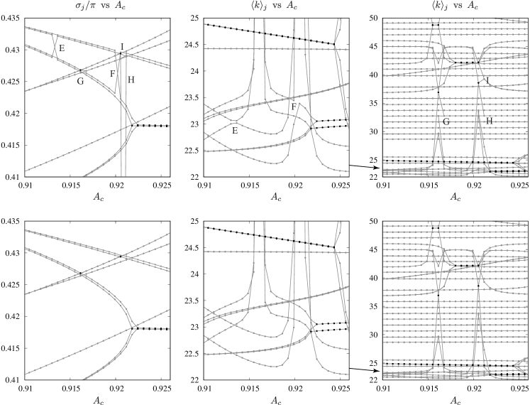
Figure 16. If the cost matrix (D.2) is modified by dropping the 1/2 powers and replacing the factor of 10 by a factor of 2, errors arise in the matching algorithm (top row) that disappear when the cost function in (D.2) is used (bottom row). Labels E, F, G, H, I show where the cost was reduced in $\langle k\rangle_{j}$ (top center and top right) at the expense of creating a criss-cross in $\sigma_{j}$ (top left).

In our initial experiments trying different formulas for $C_{ij}^{(s+1)}$ in (D.2), there were often a few criss-crossed curves such as in the top panels of Figure 16. These are easily fixed by hand (outside of matlab). We write the matrix perm to a file and create a second text file containing 3 integers per line, s,i1,i2. We wrote a short perl script to read the permutation data into memory and swap rows i1 and i2 in columns s through $\ell$ of perm. This is done repeatedly, once for each line in the second file. Finally, the perl script reads the original eigenvalue file (the file loaded by matlab to create mag, arg, kk and parity), re-orders the data according to the corrected values in perm, and writes a file with all the eigenvalues ordered properly. Finding the triples s,i1,i2 required to correct errors such as at E, F, G, H or I in the top row of Figure 16 boils down to figuring out the indices i1 and i2 associated with the two curves that cross incorrectly, and the standing wave index s where the crossing occurs. This is easily done by hand via a bisection algorithm. For each curve that incorrectly crosses to another branch of eigenvalues, we use gnuplot to plot ranges of indices in a different color, noting whether the curve in question changes color or not. Repeatedly cutting the number of curves plotted in half allows us to quickly identify the index of the desired curve. As mentioned above, the parameters in (D.2) yield correct matchings with no need for further corrections to be performed by hand.

References

- [1] T. Alazard and P. Baldi. Gravity capillary standing water waves. Arch. Rational Mech. Anal., 217:741–830, 2015.
- [2] C. J. Amick and J. F. Toland. The semi-analytic theory of standing waves. Proc. Roy. Soc. Lond. A, 411:123–138, 1987.
- [3] W. Artiles and A. Nachbin. Nonlinear evolution of surface gravity waves over highly variable depth. Phys. Rev. Lett., 93:234501, 2004.
- [4] C. H. Aurther, R. Granero-Belinchón, S. Shkoller, and J. Wilkening. Rigorous asymptotic models of water waves. Water Waves, 1(1):71–130, 2019.
- [5] G. R. Baker, D. I. Meiron, and S. A. Orszag. Generalized vortex methods for free-surface flow problems. J. Fluid Mech., 123:477–501, 1982.
- [6] G. R. Baker and C. Xie. Singularities in the complex physical plane for deep water waves. J. Fluid Mech., 685:83–116, 2011.
- [7] T. B. Benjamin and J. E. Feir. The disintegration of wave trains on deep water. part i. theory. J. Fluid Mech., 27:417–430, 1967.
- [8] T. B. Benjamin and K. Hasselmann. Instability of periodic wavetrains in nonlinear dispersive systems. Proc. R. Soc. Lond. A, 299(1456):59–76, 1967.
- [9] T. B. Benjamin and F. Ursell. The stability of the plane free surface of a liquid in vertical periodic motion. Proc. R. Soc. Lond., Ser. A, 225:505–515, 1954.
- [10] M. Berti and R. Montalto. Quasi-periodic water waves. J. Fixed Point Theory Appl., 19(1):129–156, 2017.
- [11] T. J. Bridges and F. E. Laine-Pearson. Nonlinear counterpropagating waves, multisymplectic geometry, and the instability of standing waves. SIAM J. Appl. Math., 64(6):2096–2120, 2004.
- [12] P J Bryant and M Stiassnie. Different forms for nonlinear standing waves in deep water. J. Fluid Mech., 272:135–156, 1994.
- [13] J. W. M. Bush. Pilot-wave hydrodynamics. Annu. Rev. Fluid Mech., 47:269–292, 2015.
- [14] H. D. Ceniceros and T. Y. Hou. Dynamic generation of capillary waves. Phys. Fluids, 11(5):1042–1050, 1999.
- [15] R. K.-C. Chan and R. Street. A computer study of finite amplitude water waves. J. Comput. Phys., 6:68–94, 1970.
- [16] G. A. Chandler and I. G. Graham. The computation of water waves modelled by Nekrasov’s equation. SIAM J. Numer. Anal., 30(4):1041–1065, 1993.
- [17] B. Chen and P. G. Saffman. Numerical evidence for the existence of new types of gravity waves of permanent form on deep water. Stud. Appl. Math., 62:1–21, 1980.
- [18] P. Chen. Nonlinear wave dynamics in Faraday instabilities. Phys. Rev. E, 65:036308, 2002.
- [19] Earl A. Coddington and Norman Levinson. Theory of Ordinary Differential Equations. Krieger Publishing Company, Malabar, Florida, 1984.
- [20] P. Concus. Standing capillary-gravity waves of finite amplitude. J. Fluid Mech., 14:568–576, 1962.
- [21] P. Concus. Standing capillary-gravity waves of finite amplitude: Corrigendum. J. Fluid Mech., 19:264–266, 1964.
- [22] M. J. Cooker, P. D. Weidman, and D. S. Bale. Reflection of a high-amplitude solitary wave at a vertical wall. J. Fluid Mech., 342:141–158, 1997.
- [23] W. Craig, P. Guyenne, J. Hammack, D. Henderson, and C. Sulem. Solitary water wave interactions. Phys. Fluids, 18:057106, 2006.
- [24] W. Craig and C. Sulem. Numerical simulation of gravity waves. J. Comput. Phys., 108:73–83, 1993.
- [25] A. D. D. Craik. The origins of water wave theory. Ann. Rev. Fluid Mech., 36:1–28, 2004.
- [26] A. D. D. Craik. George gabriel stokes on water wave theory. Ann. Rev. Fluid Mech., 37:23–42, 2005.
- [27] D. R. Crawford, B. M. Lake, P. G. Saffman, and H. C. Yuen. Stability of weakly nonlinear deep-water waves in two and three dimensions. J. Fluid Mech., 105:177–191, 1981.
- [28] D. F. Crouse. On implementing 2D rectangular assignment algorithms. IEEE Trans. Aerosp. Electron. Syst., 52(4):1679–1696, 2016.
- [29] B. Deconinck and K. Oliveras. The instability of periodic surface gravity waves. J. Fluid Mech., 675:141–167, 2011.
- [30] James W. Demmel. Applied Numerical Linear Algebra. SIAM, Philadelphia, 1997.
- [31] A. Dutt, L. Greengard, and V. Rokhlin. Spectral deferred correction methods for ordinary differential equations. BIT, 40(2):241–266, 2000.
- [32] A. L. Dyachenko, V. E. Zakharov, and E. A. Kuznetsov. Nonlinear dynamics on the free surface of an ideal fluid. Plasma Phys. Rep., 22:916–928, 1996.
- [33] M. Faraday. On a peculiar class of acoustical figures; and on certain forms assumed by a group of particles upon vibrating elastic surfaces. Phil. Trans. Royal Society (London), 121:299–318, 1831.
- [34] M. A. Grant. Standing Stokes waves of maximum height. J. Fluid Mech., 60:593–604, 1973.
- [35] E. Hairer, S. P. Norsett, and G. Wanner. Solving Ordinary Differential Equations I: Nonstiff Problems, 2nd Edition. Springer, Berlin, 2000.
- [36] D. M. Henderson and J. W. Miles. Faraday waves in 2:1 internal resonance. J. Fluid Mech., 222:449–470, 1991.
- [37] T. Y. Hou and R. Li. Computing nearly singular solutions using pseudo-spectral methods. J. Comput. Phys., 226:379–397, 2007.
- [38] T. Y. Hou, J. S. Lowengrub, and M. J. Shelley. Removing the stiffness from interfacial flows with surface tension. J. Comput. Phys., 114:312–338, 1994.
- [39] T. Y. Hou, J. S. Lowengrub, and M. J. Shelley. The long-time motion of vortex sheets with surface tension. Phys. Fluids, 9:1933–1954, 1997.
- [40] T. Y. Hou, J. S. Lowengrub, and M. J. Shelley. Boundary integral methods for multicomponent fluids and multiphase materials. J. Comput. Phys., 169:302–362, 2001.
- [41] J. Huang, J. Jia, and M. Minion. Accelerating the convergence of spectral deferred correction methods. J. Comput. Phys., 214:633–656, 2006.
- [42] G. Iooss, P. I. Plotnikov, and J. F. Toland. Standing waves on an infinitely deep perfect fluid under gravity. Arch. Rat. Mech. Anal., 177:367–478, 2005.
- [43] M. Ioualalen and C. Kharif. Stability of three-dimensional progressive gravity waves on deep water to superharmonic disturbances. Eur. J. Mech. B, 12:401–414, 1993.
- [44] L. Jiang, C. Ting, M. Perlin, and W. W. Schultz. Moderate and steep Faraday waves: instabilities, modulation and temporal asymmetries. J. Fluid Mech., 329:275–307, 1996.
- [45] R. S. Johnson. A modern introduction to the mathematical theory of water waves. Cambridge University Press, Cambridge, UK, 1997.
- [46] R. Jonker and A. Volgenant. A shortest augmenting path algorithm for dense and sparse linear assignment problems. Computing, 38:325–340, 1987.
- [47] R. Krasny. Desingularization of periodic vortex sheet roll-up. J. Comput. Phys., 65:292–313, 1986.
- [48] K. Kumar and L. S. Tuckerman. Parametric instability of the interface between two fluids. J. Fluid Mech., 279:49–68, 1994.
- [49] A. T. Layton and M. L. Minion. Implications of the choice of quadrature nodes for Picard integral deferred corrections methods for ordinary differential equations. BIT Numerical Mathematics, 45:341–373, 2005.
- [50] M. S. Longuet-Higgins. The instabilities of gravity waves of finite amplitude in deep water. I. superharmonics. PRoc. R. Soc. London Ser. A, 360:471–488, 1978.
- [51] M. S. Longuet-Higgins. The instabilities of gravity waves of finite amplitude in deep water. II. subharmonics. PRoc. R. Soc. London Ser. A, 360:489–505, 1978.
- [52] M. S. Longuet-Higgins. Capillary-gravity waves of solitary type on deep water. J. Fluid Mech., 200:451–478, 1989.
- [53] M. S. Longuet-Higgins and E. D. Cokelet. The deformation of steep surface waves on water. I. a numerical method of computation. Proc. Royal Soc. A, 350:1–26, 1976.
- [54] R. S. MacKay and P. G. Saffman. Stability of water waves. Proc. R. Soc. Lond. A, 406:115–125, 1986.
- [55] T. Maxworthy. Experiments on collisions between solitary waves. J. Fluid Mech., 76:177–185, 1976.
- [56] G N Mercer and A J Roberts. Standing waves in deep water: Their stability and extreme form. Phys. Fluids A, 4(2):259–269, 1992.
- [57] G N Mercer and A J Roberts. The form of standing waves on finite depth water. Wave Motion, 19:233–244, 1994.
- [58] P. A. Milewski, J.-M. Vanden-Broeck, and Z. Wang. Dynamics of steep two-dimensional gravity–capillary solitary waves. J. Fluid Mech., 664:466–477, 2010.
- [59] J. Munkres. Algorithms for the assignment and transportation problems. J. Soc. Ind. Appl. Math., 5(1):32–38, 1957.
- [60] Y. Murakami and K. Chikano. Two-dimensional direct numerical simulation of parametrically excited surface waves in viscous fluid. Phys. Fluids, 13:65–74, 2001.
- [61] D.P. Nicholls. Spectral data for travelling water waves: singularities and stability. J. Fluid Mech., 624:339–360, 2009.
- [62] J. Nocedal and S. J. Wright. Numerical Optimization. Springer, New York, 1999.
- [63] N. L. O’Connor. The complex spatiotemporal dynamics of a shallow fluid layer. Master’s thesis, Virginia Polytechnic Institute and State University, Blacksburg, VA, 2008.
- [64] M. Okamura. On the enclosed crest angle of the limiting profile of standing waves. Wave Motion, 28:79–87, 1998.
- [65] M Okamura. Standing gravity waves of large amplitude on deep water. Wave Motion, 37:173–182, 2003.
- [66] M. Okamura. Almost limiting short-crested gravity waves in deep water. J. Fluid Mech., 646:481–503, 2010.
- [67] M. Okamura, M. Ioualalen, and C. Kharif. Standing waves on water of uniform depth: on their resonances and matching with short-crested waves. J. Fluid Mech., 495:145–156, 2003.
- [68] W G Penney and A T Price. Finite periodic stationary gravity waves in a perfect liquid, part II. Phil. Trans. R. Soc. London A, 244:254–284, 1952.
- [69] N. Perinet, D. Juric, and L. S. Tuckerman. Numerical simulation of Faraday waves. J. Fluid Mech., 635:1–26, 2009.
- [70] P. Plotnikov and J. Toland. Nash-moser theory for standing water waves. Arch. Rat. Mech. Anal., 159:1–83, 2001.
- [71] S. Qadeer and J. Wilkening. Computing three-dimensional Faraday waves in a cylinder. 2019. (in preparation).
- [72] J. W. S. Rayleigh. Deep water waves, progressive or stationary, to the third order approximation. Proc. R. Soc. A, 91:345–353, 1915.
- [73] Lord Rayleigh. On the crispations of fluid resting upon a vibrating support. Phil. Mag., 16:50–58, 1883. (Reprinted in Scientific Papers, vol. 2, 1900, pp. 212–219. Cambridge).
- [74] M. M. Rienecker and J. D. Fenton. A Fourier approximation method for steady water waves. J. Fluid Mech., 104:119–137, 1981.
- [75] W W Schultz, J M Vanden-Broeck, L Jiang, and M Perlin. Highly nonlinear standing water waves with small capillary effect. J. Fluid Mech., 369:253–272, 1998.
- [76] L. W. Schwartz and J. D. Fenton. Strongly nonlinear waves. Ann. Rev. Fluid Mech., 14:39–60, 1982.
- [77] L. W. Schwartz and A. K. Whitney. A semi-analytic solution for nonlinear standing waves in deep water. J. Fluid Mech., 107:147–171, 1981.
- [78] A. C. Skeldon and G. Guidoboni. Pattern selection for Faraday waves in an incompressible viscous fluid. SIAM J. Appl. Math., 67:1064–1100, 2007.
- [79] D. H. Smith and A. J. Roberts. Branching behavior of standing waves — the signatures of resonance. Phys. Fluids, 11:1051–1064, 1999.
- [80] G. G. Stokes. Considerations relative to the greatest height of oscillatory irrotational waves which can be propagated without change of form. In Mathematical and physical papers, volume 1, pages 225–228. Cambridge University Press, 1880.
- [81] C. H. Su and R. M. Mirie. On head-on collisions between two solitary waves. J. Fluid Mech., 98:509–525, 1980.
- [82] I Tadjbakhsh and J B Keller. Standing surface waves of finite amplitude. J. Fluid Mech., 8:442–451, 1960.
- [83] G I Taylor. An experimental study of standing waves. Proc. Roy. Soc. A, 218:44–59, 1953.
- [84] O. Trichtchenko, B. Deconinck, and J. Wilkening. The instability of wilton ripples. Wave Motion, 66:147–155, 2016.
- [85] C P Tsai and D S Jeng. Numerical Fourier solutions of standing waves in finite water depth. Appl. Ocean Res., 16:185–193, 1994.
- [86] J.-M. Vanden-Broeck. Numerical calculation of standing waves in water of arbitrary uniform depth. Phys. Fluids, 24(5):812–815, 1981.
- [87] J.-M. Vanden-Broeck. Nonlinear gravity-capillary standing waves in water of arbitrary uniform depth. J. Fluid Mech., 139:97–104, 1984.
- [88] J.-M. Vanden-Broeck and F. Dias. Gravity-capillary solitary waves in water of infinite depth and related free-surface flows. J. Fluid Mech., 240:549–557, 1992.
- [89] Jean-Marc Vanden-Broeck. Gravity–Capillary Free–Surface Flows. Cambridge University Press, Cambridge, 2010.
- [90] J. M. Vega, E. Knobloch, and C. Martel. Nearly inviscid Faraday waves in annular containers of moderately large aspect ratio. Physica D, 154:313–336, 2001.
- [91] G. B. Whitham. Linear and Nonlinear Waves. Wiley, New York, 1974.
- [92] J. Wilkening. An algorithm for computing Jordan chains and inverting analytic matrix functions. Linear Algebra Appl., 427:6–25, 2007.
- [93] J. Wilkening. Breakdown of self-similarity at the crests of large amplitude standing water waves. Phys. Rev. Lett, 107:184501, 2011.
- [94] J. Wilkening. Relative-periodic elastic collisions of water waves. Contemp. Math., 635:109–129, 2015.
- [95] J. Wilkening. Long-time dynamics of water waves near stable and unstable standing waves. 2019. (in preparation).
- [96] J. Wilkening. Traveling-standing water waves and their stability. 2019. (in preparation).
- [97] J. Wilkening and J. Yu. Overdetermined shooting methods for computing standing water waves with spectral accuracy. Comput. Sci. Disc., 5:014017:1–38, 2012.
- [98] J. Wright, S. Yon, and C. Pozrikidis. Numerical studies of two-dimensional Faraday oscillations of inviscid fluids. J. Fluid Mech., 400:1–32, 2000.
- [99] W. Zhang and J. Viñals. Pattern formation in weakly damped parametric surface waves. J. Fluid Mech., 336:301–330, 1997.