The transiting multi-planet system HD 15337: two nearly equal-mass planets straddling the radius gap

Abstract

We report the discovery of a super-Earth and a sub-Neptune transiting the star HD 15337 (TOI-402, TIC 120896927), a bright ($V$ = 9) K1 dwarf observed by the Transiting Exoplanet Survey Satellite (TESS) in Sectors 3 and 4. We combine the TESS photometry with archival HARPS spectra to confirm the planetary nature of the transit signals and derive the masses of the two transiting planets. With an orbital period of 4.8 days, a mass of $7.51_{-1.01}^{+1.09}$ $M_{\oplus}$, and a radius of $1.64\pm 0.06$ $R_{\oplus}$, HD 15337 b joins the growing group of short-period super-Earths known to have a rocky terrestrial composition. The sub-Neptune HD 15337 c has an orbital period of 17.2 days, a mass of $8.11_{-1.69}^{+1.82}$ $M_{\oplus}$, and a radius of $2.39\pm 0.12$ $R_{\oplus}$, suggesting that the planet might be surrounded by a thick atmospheric envelope. The two planets have similar masses and lie on opposite sides of the radius gap, and are thus an excellent testbed for planet formation and evolution theories. Assuming that HD 15337 c hosts a hydrogen-dominated envelope, we employ a recently developed planet atmospheric evolution algorithm in a Bayesian framework to estimate the history of the high-energy (extreme ultraviolet and X-ray) emission of the host star. We find that at an age of 150 Myr, the star possessed on average between 3.7 and 127 times the high-energy luminosity of the current Sun.

1 Introduction

Successfully launched in April 2018, NASA’s Transiting Exoplanet Survey Satellite (TESS) is making a significant step forward in understanding the diversity of exoplanets, and especially of super-Earths ($R_{\mathrm{p}}$ = 1–2 R_⊕) and sub-Neptunes ($R_{\mathrm{p}}$ = 2–4 R_⊕). TESS is performing an all-sky photometric search for planets transiting bright stars ($6<V<11$), so that detailed characterizations of the planets and their atmospheres can be performed (Ricker et al., 2015). The survey is broken up into 26 sectors – each sector being observed for $\sim$28 days and consisting of four cameras with a combined field of view of $24^{\circ}$$\times$$96^{\circ}$. Candidate alerts and full-frame images are released every month. As of March 2019, TESS has already announced the discovery of about a dozen transiting planets (see, e.g., Esposito et al., 2019; Gandolfi et al., 2018; Huang et al., 2018; Jones et al., 2018; Nielsen et al., 2019; Quinn et al., 2019; Trifonov et al., 2019).

TESS has already led to the detection of “golden” systems amenable to in-depth characterization of planetary atmospheres, such as $\pi$ Men, which is a bright ($V$ = 5.65) star hosting a transiting super-Earth with a bulk density that is consistent with either a primary, hydrogen-dominated atmosphere, or a secondary, probably CO₂/H₂O-dominated, atmosphere (Gandolfi et al., 2018; Huang et al., 2018). The discovery of such systems is central for studying planetary atmospheres via multi-wavelength transmission spectroscopy, and for constraining the evolution models of planetary atmospheres.

TESS also enables the discovery of multi-planet systems for which both mass and radius can be precisely measured. Because such planets orbit the same star, differences in mean density and atmospheric structure among planets belonging to the same system can be ascribed mainly to differences in planetary mass and orbital separation (see, e.g., Guenther et al., 2017; Prieto-Arranz et al., 2018). This greatly simplifies modeling of their past evolution history, thus constraining how these planets formed (Alibert et al., 2005; Alibert & Benz, 2017). In this respect, even more significant are multi-planet systems in which two or more planets have similar masses, as differences in radii would most likely be due to the different orbital separations.

In this Letter we report the discovery of two small planets transiting the bright ($V$ = 9) star HD 15337 (Table 1), a K1 dwarf observed by TESS in Sectors 3 and 4. We combined the TESS photometry with archival HARPS radial velocities (RVs) to confirm the planetary nature of the transit signals and derive the masses of the two planets. This Letter is organized as follows. In Sect. 2, we describe the TESS photometry and the detection of the transit signals. In Sect. 3, we present the archival HARPS spectra. The properties of the host star are reported in Sect. 4. We present the frequency analysis of the HARPS RVs in Sect. 5 and the data modeling in Sect. 6. Results, discussions, and a summary are given in Sect. 7.

Table 1: Main identifiers, coordinates, proper motion, parallax, distance, and optical and infrared magnitudes of HD 15337.

Parameter	Value	Source
Main Identifiers
HD	15337
HIP	11433	Hipparcos
TIC	120896927	TICa
TOI	402	TESS Alerts
Gaia DR2	5068777809824976256	Gaia DR2b
Equatorial Coordinates
R.A. (J2000.0)	$02^{\mathrm{h}}\,27^{\mathrm{m}}\,28.3781^{\mathrm{s}}$	Gaia DR2b
Decl. (J2000.0)	$-$27∘ 38′ 06.7417${\arcsec}$	Gaia DR2b
Proper Motion, Parallax, and Distance
$\mu_{\alpha}\cos\delta$ (mas  yr-1)	$-73.590\pm 0.057$	Gaia DR2b
$\mu_{\delta}$ (mas  yr-1)	$-211.614\pm 0.082$	Gaia DR2b
Parallax (mas)	$22.285\pm 0.035$	Gaia DR2b
Distance (pc)	$44.874\pm 0.070$	Gaia DR2b
Magnitudes
$B_{\mathrm{T}}$	$10.170\pm 0.027$	Tycho-2c
$V_{\mathrm{T}}$	$9.184\pm 0.018$	Tycho-2c
$B$	$10.009\pm 0.090$	APASSd
$V$	$9.096\pm 0.017$	APASSd
$g$	$9.852\pm 0.493$	APASSd
$r$	$8.847\pm 0.016$	APASSd
$i$	$8.655\pm 0.054$	APASSd
$u$	$11.756\pm 0.075$	Strömgrene
$v$	$10.526\pm 0.046$	Strömgrene
$b$	$9.598\pm 0.032$	Strömgrene
$y$	$9.088\pm 0.030$	Strömgrene
$G$	$8.8560\pm 0.0002$	Gaia DR2b
$G_{\mathrm{BP}}$	$9.3194\pm 0.0011$	Gaia DR2b
$G_{\mathrm{RP}}$	$8.2708\pm 0.0016$	Gaia DR2b
$J$	$7.553\pm 0.019$	2MASSf
$H$	$7.215\pm 0.034$	2MASSf
$K_{s}$	$7.044\pm 0.018$	2MASSf
$W1$(3.35 $\mu$m)	$6.918\pm 0.054$	ALLWISEg
$W2$(4.6 $\mu$m)	$7.048\pm 0.020$	ALLWISEg
$W3$(11.6 $\mu$m)	$7.015\pm 0.017$	ALLWISEg
$W4$(22.1 $\mu$m)	$6.916\pm 0.072$	ALLWISEg

2 TESS photometry

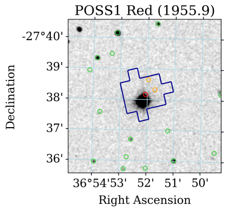
Figure 1: 5 ′ $\times$ 5 ′ 103aE emulsion image taken in 1955 from the First Palomar Sky Survey (POSS1-E), with the Sector 4 SPOC photometric aperture overplotted in blue (TESS  pixel size is 21″), and the positions of Gaia DR2 sources (J2015.5) within 2′ of HD 15337 indicated by circles. HD 15337 is in red, nearby sources contributing more than 1% of their flux to the aperture are in orange, and other sources are in green; the Sector 3 aperture is slightly bigger but yields similarly low levels of photometric dilution

(see Sect. 2). Due to the proper motion of HD 15337, there is a $\sim$14″ offset between its Gaia position and its position in the image.

HD 15337 (TIC 120896927) was observed by TESS Camera #2 in Sectors 3 and 4 (charge-coupled devices #3 and #4, respectively) from 20 September 2018 to 15 November 2018, and will not be observed further during the nominal two-year TESS mission. Photometry was interrupted when the satellite was re-pointed for data downlink, from BJD${}_{\mathrm{TDB}}=2458395.4$ to BJD${}_{\mathrm{TDB}}=2458396.6$ in Sector 3, and from BJD${}_{\mathrm{TDB}}=2458423.5$ to BJD${}_{\mathrm{TDB}}=2458424.6$ in Sector 4. There is an additional data gap in Sector 4 from BJD${}_{\mathrm{TDB}}=2458418.5$ to BJD${}_{\mathrm{TDB}}=2458421.2$, which was caused by an interruption in communications between the instrument and spacecraft.

TESS objects of interest (TOIs) are announced publicly via the TESS data alerts web portal at the Massachusetts Institute of Technology. TOIs 402.01 (HD 15337 b) and 402.02 (HD 15337 c) were announced on 16 January 2019 and 31 January 2019, respectively, in association with the HD 15337 photometry. The TESS pixel data and light curves produced by the Science Processing Operations Center (SPOC; Jenkins et al., 2016) at NASA Ames Research Center were subsequently made publicly available via the Mikulski Archive for Space Telescopes (MAST). We iteratively searched the SPOC light curves for transit signals using the Box-least-squares algorithm (BLS; Kovács et al., 2002), after fitting and removing stellar variability using a cubic spline with knots every 1.0 day. We recovered two signals corresponding to the TOIs, but no other significant signals were detected. We also tried removing variability using the wavelet-based filter routines VARLET and PHALET, but it did not change the BLS results; we are thus confident that the two signals are robustly detected and are not the result of data artifacts resulting from the choice of variability model or residual instrumental systematic signals.

The SPOC light curves are produced using automatically selected optimal photometric apertures. We also produced light curves from the TESS pixel data using a series of apertures (Gandolfi et al., 2018; Esposito et al., 2019), and found that apertures larger than the SPOC aperture shown in Fig. 1 minimized the 6.5 hr combined differential photometric precision (CDPP) noise metric (Christiansen et al., 2012). However, the transit signals recovered from these light curves were slightly less significant, which we attributed to the improvement in light curve quality afforded by the Presearch Data Conditioning (Smith et al., 2012; Stumpe et al., 2012) pipeline used by the SPOC, which corrects for common-mode systematic noise; for this reason, we opted to analyze the SPOC light curves for the remainder of the analysis in this Letter.

To investigate the possibility of diluting flux from stars other than HD 15337, we visually inspected archival images and compared Gaia DR2 (Gaia Collaboration et al., 2018) source positions with the SPOC photometric apertures. We used the coordinates of HD 15337 from the TESS Input Catalog (Stassun et al., 2018b) to retrieve Gaia DR2 sources using a search radius of 3′. In an archival image taken in 1955 from the Firs Palomar Sky Survey (POSSI-E), HD 15337 is offset from its current position by $\sim$14″ due to proper motion, but this is not sufficient to completely rule out chance alignment with a background source; however, such an alignment with a bright source is highly unlikely. Assuming the TESS point spread function (PSF) can be approximated by a two-dimensional Gaussian profile with a full-width at half maximum (FWHM) of $\sim$25″, we found that 98.9% (98.5%) of the flux from HD 15337 is within the Sector 3 (Sector 4) SPOC aperture. Approximating the TESS bandpass with the Gaia $G_{\mathrm{RP}}$ bandpass, the transit signals from HD 15337 should be diluted by less than 0.01% in both apertures; HD 15337 is the only star bright enough to be the source of the transit signals. Two other Gaia DR2 sources (5068777809825770112 and 5068777745400963584) also contribute flux, but they are too faint to yield significant dilution ($G_{\mathrm{RP}}\approx 19$ mag). Fig. 1 shows the archival image, along with Gaia  DR2 source positions and the Sector 4 SPOC photometric aperture.

3 HARPS spectroscopic observations

HD 15337 was observed between 15 December 2003 and 06 September 2017 UT with the High Accuracy Radial velocity Planet Searcher (HARPS) spectrograph (R $\approx$ 115 000, Mayor et al., 2003) mounted at the ESO-3.6 m telescope, as part of the observing programs 072.C-0488, 183.C-0972, 192.C-0852, 196.C-1006, and 198.C-0836. We retrieved the publicly available reduced spectra from the ESO archive, along with the cross-correlation function (CCF) and its bisector, computed from the dedicated HARPS pipeline using a K5 numerical mask (Baranne et al., 1996). On June 2015, the HARPS fiber bundle was upgraded and a new set of octagonal fibers, with improved mode-scrambling capabilities, were installed (Lo Curto et al., 2015). To account for the RV offset caused by the instrument refurbishment, we treated the HARPS RVs taken before/after June 2015 as two different data sets. Tables 3 and 4 list the HARPS RVs taken with the old and new fiber bundle, along with the RV uncertainties, the full-width at half maximum (FWHM) and bisector span (BIS) of the CCF, the exposure times, and the signal-to-noise ratio (S/N) per pixel at 5500 Å. Time stamps are given in barycentric Julian Date in the barycentric dynamical time (BJD _TDB). We rejected two data points – marked with asterisks in Tables 3 and 4 – because of poor S/N ratio (BJD_TDB = 2455246.519846) or systematics (BJD_TDB = 2457641.794439).

4 Stellar fundamental parameters

4.1 Spectroscopic parameters

We co-added the HARPS spectra obtained with the old and new fiber bundle separately to get two combined spectra with S/N per pixel at 5500 Å of 590 (old fiber) and 490 (new fiber). We derived the spectroscopic parameters of HD 15337 from the co-added HARPS spectra using Spectroscopy Made Easy (SME), a spectral analysis tool that calculates synthetic spectra and fits them to high-resolution observed spectra using a $\chi^{2}$ minimizing procedure. The analysis was performed with the non-local thermodynamic equilibrium (non-LTE) SME version 5.2.2, along with MARCS model atmospheres (Gustafsson et al., 2008).

We estimated a microturbulent velocity of $v_{\rm mic}$=$0.80\pm 0.10$ $\mathrm{km\,s^{-1}}$ from the empirical calibration equations for Sun-like stars from Bruntt et al. (2010). The effective temperature $T_{\rm eff}$ was measured fitting the wings of the H_α and H_β lines, as well as the Na i doublet at 5890 and 5896 Å (Fuhrmann et al., 1993; Axer et al., 1994; Fuhrmann et al., 1994, 1997b, 1997a). The surface gravity log g_⋆ was determined from the wings of the Ca i $\lambda$ 6102, $\lambda$ 6122, $\lambda$ 6162 Å triplet, and the Ca i $\lambda$ 6439 Å line, as well as from the Mg i $\lambda$ 5167, $\lambda$ 5173, $\lambda$ 5184 Å triplet. We measured the iron abundance [Fe/H], the macroturbulent velocity $v_{\rm mac}$, and the projected rotational velocity $v$ sin $i_{\star}$ by simultaneously fitting the unblended iron lines in the spectral region 5880–6600 Å.

Our analyses applied to the two stacked HARPS spectra provided consistent results, well within the uncertainties. The final adopted values are listed in Table 2. We derived an effective temperature of $T_{\rm eff}$=5125$\pm$50 K, surface gravity log g_⋆=$4.40\pm 0.10$ (cgs), and an iron abundance relative to solar of [Fe/H]=$0.15\pm 0.08$ dex. We also measured a calcium abundance of [Ca/H]=$0.16\pm 0.05$ dex and a sodium abundance of [Na/H]=$0.27\pm 0.09$ dex. We found a macroturbulent velocity of $v_{\rm mac}$=$3.0\pm 1.0$ km/s in agreement with the value predicted from the empirical equations of Doyle et al. (2014). The projected rotational velocity was found to be $v$ sin $i_{\star}$=$1.0\pm 1.0$ $\mathrm{km\,s^{-1}}$.

4.2 Stellar mass, radius, age and interstellar extinction

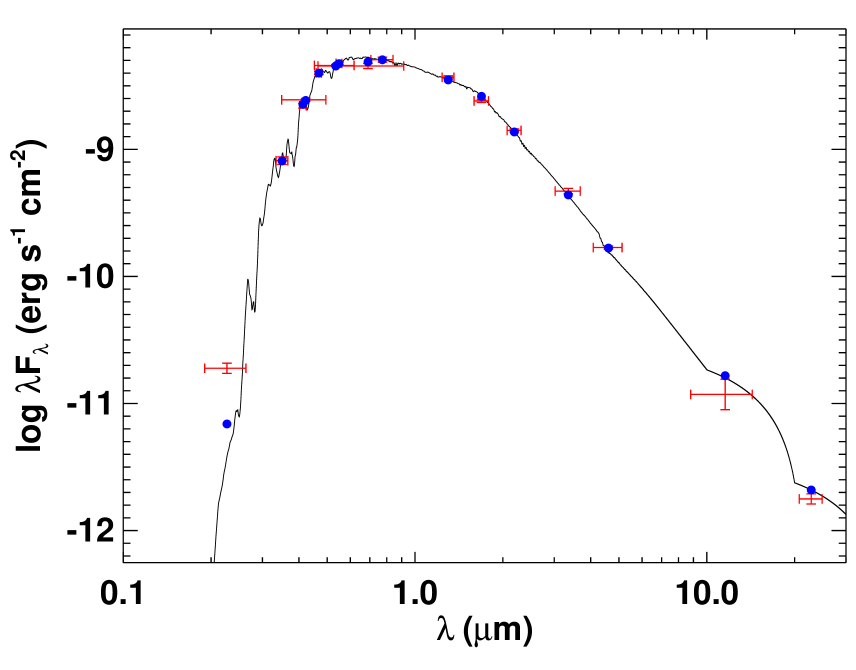
Figure 2: Spectral energy distribution (SED) of HD 15337. Red symbols represent the observed photometric measurements, where the horizontal bars represent the effective width of the passband. Blue symbols are the model fluxes from the best-fit Kurucz atmosphere model (black).

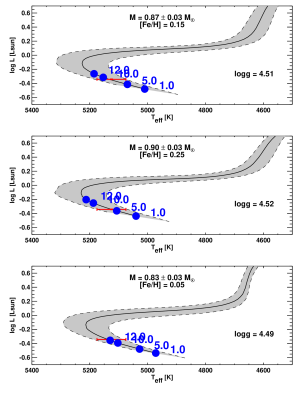
Figure 3: Hertzsprung–Russell Diagram for HD 15337 based on the observed effective temperature and bolometric luminosity, the latter computed directly from $F_{\rm bol}$ and the Gaia parallax-based distance. Each panel compares the observed properties of the star to evolutionary tracks from the Yonsei–Yale models (Yi et al., 2001; Spada et al., 2013) for different permitted combinations of stellar mass and metallicity. Blue points with labels represent the model ages in Gyr. The central panel represents the case most compatible with all of the available data, including the stellar age of $\approx$5.1 Gyr as determined from the observed chromospheric activity and stellar rotation period (see the text).

We performed an analysis of the broadband spectral energy distribution (SED) together with the Gaia Data Release 2 (DR2; Gaia Collaboration et al., 2018) parallax in order to determine an empirical measurement of the stellar radius, following the procedures described in Stassun & Torres (2016), Stassun et al. (2017), and Stassun et al. (2018a). We retrieved the $B_{\mathrm{T}}$ and $V_{\mathrm{T}}$ magnitudes from Tycho-2 catalog (Høg et al., 2000), the Strömgren $ubvy$ magnitudes from Paunzen (2015), the $BVgri$ magnitudes from APASS (Henden et al., 2015), the $JHK_{S}$ magnitudes from 2MASS (Cutri et al., 2003), the $W1$–$W4$ magnitudes from ALLWISE (Cutri, 2013), and the $G$ magnitude from Gaia DR2 (Gaia Collaboration et al., 2018). Together, the available photometry spans the full stellar SED over the wavelength range 0.35–22 $\mu$m (Table 1 and Fig. 2). In addition, we retrieved the near-ultraviolet (NUV) flux from the Galaxy Evolution Explorer (GALEX) survey (Bianchi et al., 2011) in order to assess the level of chromospheric activity, if any.

We performed a fit using Kurucz stellar atmosphere models (Castelli & Kurucz, 2003), with the fitted parameters being the effective temperature $T_{\rm eff}$ and iron abundance [Fe/H], as well as the interstellar extinction $A_{\mathrm{v}}$, which we restricted to the maximum line-of-sight value from the dust maps of Schlegel et al. (1998). The broadband SED is largely insensitive to the surface gravity (log g_⋆), thus we simply adopted the value from the initial spectroscopic analysis presented in the previous subsection. The resulting fit (Fig. 2) gives a reduced $\chi^{2}$ of 2.3 (excluding the GALEX NUV flux, which is consistent with a modest level of chromospheric activity). The best-fitting effective temperature and iron content are $T_{\rm eff}$ = 5130 $\pm$ 50 K and [Fe/H] = $0.1_{-0.1}^{+0.2}$ dex, respectively, in excellent agreement with the spectroscopic values (Sect. 4.1 and Table 2). We found that the reddening of HD 15337 is consistent with zero ($A_{\mathrm{v}}$ = 0.02 $\pm$ 0.02 mag), as expected given the relatively short distance to the star ($\sim$45 pc). Integrating the unreddened model SED gives a bolometric flux at Earth of $F_{\rm bol}=7.29\pm 0.08\times 10^{-9}$ erg s cm^-2. Taking the $F_{\rm bol}$ and $T_{\rm eff}$ together with the Gaia DR2 parallax, adjusted by $+0.08$ mas to account for the systematic offset reported by Stassun & Torres (2018), gives the stellar radius as $R_{\star}$ = 0.856 $\pm$ 0.017 $R_{\odot}$. Finally, estimating the stellar mass from the empirical relations of Torres et al. (2010) and a 6% error from the empirical relation itself gives a stellar mass of $M_{\star}$ = 0.91 $\pm$ 0.06 $M_{\odot}$.

We can refine the stellar mass estimate by taking advantage of the observed chromospheric activity, which can constrain the age of the star via empirical relations. For example, taking the chromospheric activity indicator, $\log R^{\prime}_{\mathrm{HK}}$ = $-4.916$ $\pm$0.038 from Gomes da Silva et al. (2014) and applying the empirical relations of Mamajek & Hillenbrand (2008), gives a predicted age of 5.1 $\pm$ 0.8 Gyr. As shown in Fig. 3, according to the Yonsei–Yale stellar evolutionary models (Yi et al., 2001; Spada et al., 2013), this age is most compatible with a stellar mass of $M_{\star}$ = 0.90 $\pm$ 0.03 $M_{\odot}$ and [Fe/H] = 0.25 dex, which with the empirically determined stellar radius implies a stellar log g_⋆ = 4.53 $\pm$ 0.02 (cgs) – in good agreement with the spectroscopic value of log g_⋆ = 4.40 $\pm$ 0.10 (cgs).

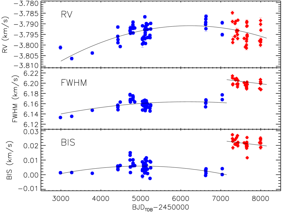
Figure 4: Offset-corrected HARPS RVs of HD 15337 (upper panel), and FWHM and BIS of the cross-correlation function (middle and lower panels). The blue circles and red diamonds mark the measurements acquired with the old and new fiber bundle, respectively. The thick lines mark the best-fitting parabolic curves to the data (see the text).

Other combinations of stellar mass and metallicity are compatible with the observed effective temperature and radius (Fig. 3); however they require ages that are incompatible with that predicted by the chromospheric $R^{\prime}_{\mathrm{HK}}$ emission. Finally, we can further corroborate the activity-based age estimate by also using empirical relations to predict the stellar rotation period from the activity. For example, the empirical relation between $R^{\prime}_{\mathrm{HK}}$ and rotation period from Mamajek & Hillenbrand (2008) predicts a rotation period for this star of $\approx$42 days, which is compatible with the observed rotation period derived from the HARPS RVs and activity indicators ($P_{\mathrm{rot}}$ = 36.5 days; see the following section).

5 Frequency analysis of the HARPS measurements

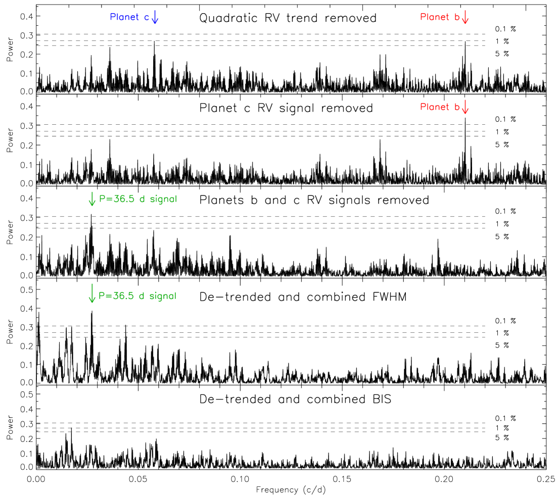
Figure 5: Generalized Lomb–Scargle periodograms of (1) the combined HARPS RV measurements, following the subtraction of the quadratic trend (first panel); (2) the RV residuals after subtracting the signal of HD 15337 c (second panel); (3) the RV residuals after subtracting the signal of HD 15337 b and c (third panel); (4) the FWHM of the cross-correlation function (fourth panel); (5) the bisector span (BIS) of the cross-correlation function (fifth panel). The dashed horizontal lines mark the FAP at 0.1%, 1% and 5 %. The frequencies of the two transiting planets, as well as of the signal at 36.5 days are marked with vertical arrows.

We performed a frequency analysis of the HARPS time-series to search for the Doppler reflex motion induced by the two transiting planets discovered by TESS. We accounted for the RV offset between the two different set-ups of the instrument (old and new fiber bundle) using the value of 19.7 $\mathrm{m\,s^{-1}}$ derived from the joint analysis presented in Sect. 6, which is in good agreement with the expected offset for a slowly rotating K1 V star such as HD 15337 (Lo Curto et al., 2015).

The offset-corrected HARPS RVs are displayed in Fig. 4 (upper panel), along with the time-series of the full-width at half maximum (FWHM; middle panel) and bisector span (BIS; lower panel). The generalized Lomb–Scargle (GLS) periodogram (Zechmeister & Kürster, 2009) of the combined RV data shows significant power at frequencies lower than the inverse of the temporal baseline of the HARPS observations, which is visible as a quadratic trend in the upper panel of Fig. 4. A similar trend is observed in the FWHM obtained with the old fiber bundle (middle panel, blue circles), suggesting that the RV trend might be due to long-term stellar variability (e.g., magnetic cycles). Alternatively, the RV trend might be induced by a long period orbiting companion, while the long-term variation of the FWHM might be ascribable to the steady instrument de-focusing observed between 2004 and 2015 (Lo Curto et al., 2015).

The upper panel of Fig. 5 shows the GLS periodogram of the combined HARPS RVs, following the subtraction of the best-fitting quadratic trend (cfr. Fig. 4). The peaks with the highest power are found at the orbital frequencies of the two transiting planets ($f_{c}$ = 0.058 c/d and $f_{b}$ = 0.210 c/d), with false-alarm probabilities (FAPs) of $\approx$ 1% and RV semi-amplitude of about 2.0-2.5 $\mathrm{m\,s^{-1}}$. The periodogram of the RV residuals after subtracting the signal of the outer planet (Fig. 5, second panel), shows a significant peak (FAP $<$ 0.1 %) at the frequency of the inner planet. The two peaks have no counterparts in the periodograms of the activity indicators (FWHM and BIS; Fig. 5, fourth and fifth panels), suggesting that the signals are induced by two orbiting planets with periods of 4.8 and 17.2 days. Finally, the GLS periodogram of the RV residuals after subtracting the quadratic trend and the signals of the two planets (Fig. 5, third panel) displays a peak with a FAP $<$ 0.1 % at $\sim$36.5 days, which is also significantly detected in the periodogram of the FWHM (fourth panel). We interpreted the 36.5 days signal as the rotation period of the star, which agrees with the value expected from the $R^{\prime}_{\mathrm{HK}}$ activity indicator (Sect. 4.2).

6 Joint analysis

We performed a joint analysis of the TESS light curve (Sect. 2) and RV measurements (Sect. 3) using the software suite pyaneti, which allows for parameter estimation from posterior distributions calculated using Markov chain Monte Carlo (MCMC) methods.

We removed stellar variability from the TESS light curves using a cubic spline with knots spaced every 1.5 days. We then extracted $\sim$8 hours of TESS photometry centered on each of the nine (HD 15337 b) and three (HD 15337 c) transits observed by TESS during Sectors 3 and 4. As described in Sect. 3, we rejected two HARPS RVs and used the remaining 85 Doppler measurements, while accounting for an RV offset between the two different HARPS set-ups.

The RV model includes a linear and a quadratic term, to account for the long-term variation described in Sect. 5, as well as two Keplerians, to account for the Doppler reflex motion induced by HD 15337 b and HD 15337 c. The RV stellar signal at the star’s rotation period was modeled as an additional coherent sine-like curve whose period was constrained with a uniform prior centered at $P_{\mathrm{rot}}$ = 36.5 days and having a width of 0.2 day, as derived from the FWHM of the peak detected in the periodogram of the HARPS FWHMs. For the phase and amplitude of the activity signal we adopted uniform priors. While this simple model might not fully reproduce the periodic and quasi-periodic variations induced by evolving active regions carried around by stellar rotation, it has proven to be effective in accounting for the stellar signal of active and moderately active stars (e.g., Pepe et al., 2013; Gandolfi et al., 2017; Barragán et al., 2018; Prieto-Arranz et al., 2018). Any variation not properly modeled by the coherent sine-curve, and/or any instrumental noise not included in the nominal RV uncertainties, were accounted for by fitting two RV jitter terms for the two HARPS set-ups.

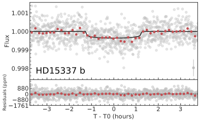
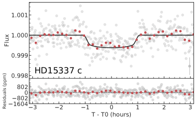
Figure 6: Folded transit light curves of HD 15337 b (left panel) and HD 15337 c (middle panel), based on nice and three single transits observed by TESS. The best-fitting transit models are overplotted with thick black lines. The TESS data points are shown with gray circles, whereas the 10 minutes binned data are displayed with red circles.

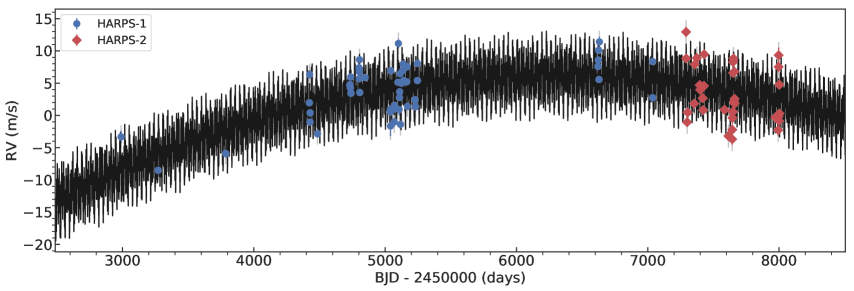
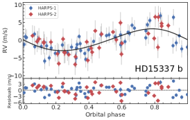
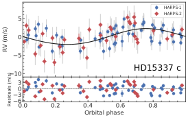
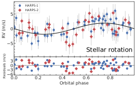
Figure 7: Upper panel: HARPS RV measurements vs. time, following the subtraction of the systemic velocities derived for the old (blue circles) and new (red diamonds) instrument set-up. Lower panels: phase-folded RV curves of HD 15337 b (left), HD 15337 c (middle) and stellar signal at 36.5 days (right). The best-fitting Keplerian and sine models are overplotted with thick black lines. The vertical gray lines mark the error bars including the RV jitter.

We modeled the TESS transit light curves using the limb-darkened quadratic model of Mandel & Agol (2002). For the limb-darkening coefficients, we set Gaussian priors using the values derived by Claret (2017) for the TESS passband. We imposed conservative error bars of 0.1 on both the linear and quadratic limb-darkening terms. For the eccentricity and argument of periastron we adopted the parametrization proposed by Anderson et al. (2011). A preliminary analysis showed that the transit light curve poorly constrains the scaled semi-major axis ($a/R_{\star}$). We therefore set a Gaussian prior on $a/R_{\star}$ using Kepler’s third law, the orbital period, and the derived stellar mass and radius (Sect. 4.2). We imposed uniform priors for the remaining fitted parameters. Details of the fitted parameters and prior ranges are given in Table 2. We used 500 independent Markov chains initialized randomly inside the prior ranges. Once all chains converged, we used the last 5000 iterations and saved the chain states every 10 iterations. This approach generates a posterior distribution of 250,000 points for each fitted parameter. Table 2 lists the inferred planetary parameters. They are defined as the median and 68% region of the credible interval of the posterior distributions for each fitted parameter. The transit and RV curves are shown in Fig. 6 and Fig. 7, along with the best-fitting models.

We also experimented with Gaussian Processes (GPs) to model the correlated RV noise associated with stellar activity. GPs model stochastic processes with a parametric description of the covariance matrix. GP regression has proven to be successful in modeling the effect of stellar activity for several other exoplanetary systems (see, e.g., Haywood et al., 2014; Grunblatt et al., 2015; López-Morales et al., 2016; Barragán et al., 2018). To this aim, we modified the code pyaneti in order to include a GP algorithm coupled to the MCMC method. We implemented the GP approach proposed by Rajpaul et al. (2015). Briefly, this framework assumes that the star-induced RV variations and activity indicators can be modeled by the same underlying GP and its derivative. This allows the GP to disentangle the RV activity component from the planetary signals.

We assumed that the stellar activity can be modeled by the quasi-periodic kernel described by Rajpaul et al. (2015). We modeled together the HARPS RV, BIS, and FWHM time-series and we treated RV and BIS as being described by the GP and its first derivative, while for FWHM we assumed that it is only described by the GP. The fitted hyper-parameters are then $V_{c}$, $V_{r}$, $B_{c}$, $B_{r}$, $L_{c}$, as defined by Rajpaul et al. (2015), to account for the GP amplitudes of the RV, BIS, and FWHM signals, the period of the activity signal $P_{\rm GP}$, the inverse of the harmonic complexity $\lambda_{\rm p}$, and the long term evolution timescale $\lambda_{\rm e}$. We coupled this GP approach with the joint modeling described in the previous paragraphs of the present section (omitting the extra coherent signal).

As for the planetary signals, we imposed the same priors listed in Table 2. For the hyper-parameters, we used uniform priors, except for $P_{\rm GP}$, for which we imposed a Gaussian prior with mean 36.5 days and standard deviation of 0.2 day. We used 250 chains to explore the parameter space. We created the posterior distributions with 500 iterations of converged chains, which generated a posterior distribution with 250,000 points for each parameters.

For planets b and c we derived an RV semi-amplitude of $2.71_{-0.51}^{+0.54}$ $\mathrm{m\,s^{-1}}$and $2.06_{-0.58}^{+0.64}$ $\mathrm{m\,s^{-1}}$, respectively, which are in very good agreement with the values reported in Table 2. The other planetary and orbital parameters are also consistent with the values presented in Table 2. For the GP hyper-parameters, we found $V_{c}=0.55\pm 0.23$ $\mathrm{m\,s^{-1}}$, $V_{r}=70_{-21}^{+27}$ $\mathrm{m\,s^{-1}}$, $B_{c}=9.4_{-2.9}^{+3.4}$ $\mathrm{m\,s^{-1}}$, $B_{r}=64_{-25}^{+20}$ $\mathrm{m\,s^{-1}}$, $L_{c}=5.4\pm 2.2$ $\mathrm{m\,s^{-1}}$  $P_{\rm GP}=36.5\pm 0.2$ d, $\lambda_{\rm e}=4217_{-685}^{+624}$ d, and $\lambda_{\rm p}=1086_{-394}^{+501}$. The relatively large values of the scale parameters in the GP, i.e. $\lambda_{\rm e}$ and $\lambda_{\rm p}$, indicate that the stellar activity behaves like a sinusoidal signal (with slight corrections).

7 Discussion and conclusions

The innermost transiting planet HD 15337 b ($P_{\mathrm{orb,b}}=4.8$ days) has a mass of $M_{\mathrm{b}}$=$7.51_{-1.01}^{+1.09}$ $M_{\oplus}$ and a radius of $R_{\mathrm{b}}$=$1.64\pm 0.06$ $R_{\oplus}$, yielding a mean density of $\rho_{\mathrm{b}}$=$9.30_{-1.58}^{+1.81}$ ${\rm g\,cm^{-3}}$. Figure 8 displays the position of HD 15337 b on the mass-radius diagram compared to the sub-sample of small transiting planets ($R_{\mathrm{p}}\leq 3$ $R_{\oplus}$) whose masses and radii have been derived with a precision better than 25%. Theoretical models from Zeng et al. (2016) are overplotted using different lines and colors. Given the precision of our mass determination ($\sim$14%), we conclude that HD 15337 b is a rocky terrestrial planet with a composition consisting of $\sim$50 % silicate and $\sim$50% iron.

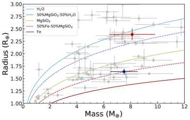
Figure 8: Mass–radius diagram for low-mass ($M_{\rm p}$ $<$ 12 $M_{\oplus}$), small ($R_{\rm p}$ $<$ 3 $R_{\oplus}$) planets with mass-radius measurements better than 25% (from http://www.astro.keele.ac.uk/jkt/tepcat/; Southworth, 2011). Composition models from Zeng et al. (2016) are displayed with different lines and colors. The solid blue and red circles mark the position of HD 15337 b and HD 15337 c, respectively.

For HD 15337 c ($P_{\mathrm{orb,c}}$=17.2 days), we obtained a mass of $M_{\mathrm{c}}$=$8.11_{-1.69}^{+1.82}$ $M_{\oplus}$ and a radius of $R_{\mathrm{c}}$=$2.39\pm 0.12$ $R_{\oplus}$, yielding a mean density of $\rho_{\mathrm{c}}$=$3.23_{-0.72}^{+0.90}$ ${\rm g\,cm^{-3}}$. Therefore, HD 15337 b and c have similar masses, but the radius of HD 15337 c is $\sim$1.5 times larger than the radius of HD 15337 b. The lower bulk density of HD 15337 c suggests that the planet is likely composed by a rocky core surrounded either by a considerable amount of water, or by a light, hydrogen-dominated envelope. In the case of a water-rich planet, the amount of water and high planetary equilibrium temperature would imply the presence of a steam atmosphere, which would be strongly hydrogen dominated in its upper layer, as a consequence of water dissociation and the low mass of hydrogen. It is therefore plausible to assume that HD 15337 c hosts a hydrogen-dominated atmosphere, at least in its upper part.

As in other systems hosting two close-in sub-Neptune-mass planets (e.g., HD 3167 Gandolfi et al., 2017), the radii of HD 15337 b and c lie on opposite sides of the radius gap (Fulton et al., 2017; Van Eylen et al., 2018), with the closer-in planet having a higher bulk density, similar to other close-in systems with measured planetary masses (e.g., HD 3167, K2-109, GJ 9827; Gandolfi et al., 2017; Guenther et al., 2017; Prieto-Arranz et al., 2018). This gap is believed to be caused by atmospheric escape (Owen & Wu, 2017; Jin & Mordasini, 2018), which is stronger for closer-in planets. Within this picture, HD 15337 b would probably have lost its primary, hydrogen-dominated atmosphere and now hosts a secondary atmosphere possibly resulting from out-gassing of a solidifying magma ocean, while HD 15337 c is likely to still partly retain the primordial hydrogen-dominated envelope. This is consistent with Van Eylen et al. (2018), who measured the location and slope of the radius gap as a function of orbital period and matched it to models suggesting a homogeneous terrestrial core composition.

To first order, the radii of HD 15337 b and c depend on the present-day properties of their atmospheres, which are intimately related to the amount of high-energy (X-ray and extreme ultraviolet; $\lambda<91.2$ nm) stellar radiation received since the dispersal of the protoplanetary nebula, and thus also to the stellar rotation history. The evolution of the stellar rotation rate does not follow a unique path because stars of the same mass and metallicity can have significantly different rotation rates up to about 1 Gyr (e.g., Mamajek & Hillenbrand, 2008; Johnstone et al., 2015; Tu et al., 2015). For older stars, it is therefore not possible to infer their past high-energy emission from their measured stellar properties. Starting from the assumption that HD 15337 c hosted a hydrogen-dominated atmosphere with solar metallicity throughout its entire evolution, we derived the history of the stellar rotation and high-energy emission by modeling the atmospheric evolution of HD 15337 c. To this end, we employed the atmospheric evolution algorithm described by Kubyshkina et al. (2018) and further developed by Kubyshkina et al. (2019, ApJ, in press), which is based on a Bayesian approach, fitting the currently observed planetary radius and combining the planetary evolution model with the MCMC open-source algorithm of Cubillos et al. (2017). The planetary atmospheric evolution model, system parameters (i.e., planetary mass, planetary radius, orbital separation, current stellar rotation period, stellar age, stellar mass; Table 2) were then used to compute the posterior distribution for the stellar rotation rate at any given age via MCMC. We assumed Gaussian priors determined by the measured system parameters and their uncertainties.

Figure 9 shows the obtained posterior distribution for the rotation period HD 15337 at an age of 150 Myr in comparison with the distribution derived from measurements of open cluster stars of the same age (Johnstone et al., 2015). Our results indicate that HD 15337, when it was young, was likely to be a moderate rotator, with a high-energy emission at 150 Myr ranging between 3.7 and 127 times the current solar emission, further excluding that the star was a very fast/slow rotator. We further employed the result shown in Fig. 9 to estimate the past atmospheric evolution of a possible hydrogen-dominated atmosphere of HD 15337 b. Accounting for all uncertainties on the system parameters and on the derived history of the stellar rotation period, we obtained that HD 15337 b has completely lost its primary atmosphere, assuming it held one, within 300 Myr, in agreement with the currently observed mean density.

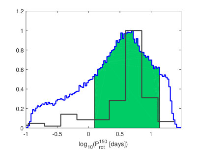
Figure 9: MCMC posterior distributions for the stellar rotation period at an age of 150 Myr obtained from the modeling of HD 15337 c. The shaded areas correspond to the 68% region of the credible interval of the posterior distribution. The black histogram shows the distribution of stellar rotation periods measured for open cluster stars with an age of 150 Myr (from Johnstone et al., 2015).

The position of HD 15337 c in the mass-radius diagram (Fig. 8) indicates that the planet may be hosting a massive hydrogen-dominated envelope or a smaller secondary atmosphere. As primary atmospheres are easily subject to escape, knowing the current composition of the envelope of HD 15337 c would provide a strong constraint on atmospheric evolution models. In this respect, this planet is similar to $\pi$ Men c (Gandolfi et al., 2018; Huang et al., 2018); furthermore, as for $\pi$ Men, the close distance to the system and brightness of the host star would enable high-quality transmission spectroscopy spanning from far-ultraviolet to infrared wavelengths. Of particular interest would be probes of an extended, escaping atmosphere. Spectral lines sensitive to various levels of extended atmospheres include H i, C ii, and O i resonance lines in the ultraviolet, H_α in the optical, and He I in the near-infrared. This suite of lines would provide a comprehensive picture of the upper atmosphere of the planet, thus constraining atmospheric escape and evolution models.

Table 2: HD 15337 System Parameters.

Parameter	Prior(a)	Derived Value
Stellar Parameters
Star mass $M_{\star}$ ($M_{\odot}$)	$\cdots$	$0.90\pm 0.03$
Star radius $R_{\star}$ ($R_{\odot}$)	$\cdots$	$0.856\pm 0.017$
Effective temperature $\mathrm{T_{eff}}$ (K)	$\cdots$	$5125\pm 50$
Surface gravity(b) log g⋆ (cgs)	$\cdots$	4.53 $\pm$ 0.02
Surface gravity(c) log g⋆ (cgs)	$\cdots$	4.40 $\pm$ 0.10
Iron abundance [Fe/H] (dex)	$\cdots$	0.15 $\pm$ 0.10
Sodium abundance [Na/H] (dex)	$\cdots$	0.27 $\pm$ 0.09
Calcium abundance [Ca/H] (dex)	$\cdots$	0.16 $\pm$ 0.05
Projected rotational velocity $v$ sin $i_{\star}$ ($\mathrm{km\,s^{-1}}$)	$\cdots$	1.0 $\pm$ 1.0
Age (Gyr)	$\cdots$	5.1 $\pm$ 0.8
Interstellar extinction $A_{\mathrm{v}}$	$\cdots$	0.02 $\pm$ 0.02
Model Parameters of HD 15337 b
Orbital period $P_{\mathrm{orb,\,b}}$ (days)	$\mathcal{U}[4.7552,4.7572]$	$4.75615\pm 0.00017$
Transit epoch $T_{\mathrm{0,\,b}}$ (BJD${}_{\mathrm{TDB}}-$2 450 000)	$\mathcal{U}[8411.4526,8411.4706]$	$8411.46156_{-0.00119}^{+0.00094}$
Scaled semi-major axis $a_{\mathrm{b}}/R_{\star}$	$\mathcal{N}[13.11,0.17]$	$13.11_{-0.15}^{+0.16}$
Planet-to-star radius ratio $R_{\mathrm{b}}/R_{\star}$	$\mathcal{U}[0,0.1]$	$0.01761_{-0.00058}^{+0.00055}$
Impact parameter $b_{\mathrm{b}}$	$\mathcal{U}[0,1]$	$0.33_{-0.14}^{+0.09}$
$\sqrt{e_{\mathrm{b}}}\sin\omega_{\mathrm{\star,\,b}}$	$\mathcal{U}[-1,1]$	$0.22_{-0.11}^{+0.09}$
$\sqrt{e_{\mathrm{b}}}\cos\omega_{\mathrm{\star,\,b}}$	$\mathcal{U}[-1,1]$	$0.12_{-0.18}^{+0.14}$
RV semi-amplitude variation $K_{\mathrm{b}}$ ($\mathrm{m\,s^{-1}}$)	$\mathcal{U}[0,10]$	$3.08_{-0.41}^{+0.44}$
Model Parameters of HD 15337 c
Orbital period $P_{\mathrm{orb,\,c}}$ (days)	$\mathcal{U}[17.1676,17.1876]$	$17.1784\pm 0.0016$
Transit epoch $T_{\mathrm{0,\,c}}$ (BJD${}_{\mathrm{TDB}}-$2 450 000)	$\mathcal{U}[8414.5416,8414.5616]$	$8414.5501\pm 0.0015$
Scaled semi-major axis $a_{\mathrm{c}}/R_{\star}$	$\mathcal{N}[31.68,0.70]$	$31.87\pm 0.70$
Planet-to-star radius ratio $R_{\mathrm{c}}/R_{\star}$	$\mathcal{U}[0,0.1]$	$0.0256\pm 0.0011$
Impact parameter $b_{\mathrm{c}}$	$\mathcal{U}[0,1]$	$0.87_{-0.02}^{+0.01}$
$\sqrt{e_{\mathrm{c}}}\sin\omega_{\mathrm{\star,\,c}}$	$\mathcal{U}[-1,1]$	$-0.08_{-0.15}^{+0.16}$
$\sqrt{e_{\mathrm{c}}}\cos\omega_{\mathrm{\star,\,c}}$	$\mathcal{U}[-1,1]$	$0.12_{-0.17}^{+0.15}$
RV semi-amplitude variation $K_{\mathrm{c}}$ ($\mathrm{m\,s^{-1}}$)	$\mathcal{U}[0,10]$	$2.16_{-0.45}^{+0.48}$
Additional Model Parameters
Parameterized limb-darkening coefficient $q_{1}$	$\mathcal{N}[0.43,0.1]$	$0.37\pm 0.08$
Parameterized limb-darkening coefficient $q_{2}$	$\mathcal{N}[0.19,0.1]$	$0.25\pm 0.11$
Systemic velocity $\gamma_{\mathrm{HS1}}$ (km s-1)	$\mathcal{U}[$-$4.0,$-$3.6]$	$-3.8174\pm 0.0027$
Systemic velocity $\gamma_{\mathrm{HS2}}$ (km s-1)	$\mathcal{U}[$-$4.0,$-$3.6]$	$-3.7977\pm 0.0012$
RV jitter term $\sigma_{\mathrm{HS1}}$ ($\mathrm{m\,s^{-1}}$)	$\mathcal{U}[0,100]$	$2.19_{-0.30}^{+0.36}$
RV jitter term $\sigma_{\mathrm{HS2}}$ ($\mathrm{m\,s^{-1}}$)	$\mathcal{U}[0,100]$	$2.89_{-0.43}^{+0.58}$
Stellar rotation period ($P_{\mathrm{rot}}$) days	$\mathcal{U}[36.4,36.6]$	$36.528\pm 0.022$
Linear RV term ${\rm m\,s^{-1}\,d^{-1}}$	$\mathcal{U}[-0.1,0.1]$	$-0.0057\times 0.0017$
Quadratic RV term ${\rm m\,s^{-1}\,d^{-1}}$	$\mathcal{U}[-0.1,0.1]$	$-13.3\pm 2.6\times 10^{-7}$
Derived Parameters of HD 15337 b
Planet mass $M_{\mathrm{b}}$ ($M_{\oplus}$)	$\cdots$	$7.51_{-1.01}^{+1.09}$
Planet radius $R_{\mathrm{b}}$ ($R_{\oplus}$)	$\cdots$	$1.64\pm 0.06$
Planet mean density $\rho_{\mathrm{b}}$ ($\mathrm{g\,cm^{-3}}$)	$\cdots$	$9.30_{-1.58}^{+1.81}$
Semi-major axis of the planetary orbit $a_{\mathrm{b}}$ (au)	$\cdots$	$0.0522\pm 0.0012$
Orbit eccentricity $e_{\mathrm{b}}$	$\cdots$	$0.09\pm 0.05$
Argument of periastron of stellar orbit $\omega_{\mathrm{\star,\,b}}$ (deg)	$\cdots$	$62_{-32}^{+42}$
Orbit inclination $i_{\mathrm{b}}$ (deg)	$\cdots$	$88.5_{-0.4}^{+0.6}$
Equilibrium temperature(d) $T_{\mathrm{eq,\,b}}$ (K)	$\cdots$	$1001\pm 11.5$
Transit duration $\tau_{\mathrm{14,\,b}}$ (hr)	$\cdots$	$2.49\pm 0.06$
Derived Parameters of HD 15337 c
Planet mass $M_{\mathrm{c}}$ ($M_{\oplus}$)	$\cdots$	$8.11_{-1.69}^{+1.82}$
Planet radius $R_{\mathrm{c}}$ ($R_{\oplus}$)	$\cdots$	$2.39\pm 0.12$
Planet mean density $\rho_{\mathrm{c}}$ ($\mathrm{g\,cm^{-3}}$)	$\cdots$	$3.23_{-0.72}^{+0.90}$
Semi-major axis of the planetary orbit $a_{\mathrm{c}}$ (au)	$\cdots$	$0.1268\pm 0.0038$
Orbit eccentricity $e_{\mathrm{c}}$	$\cdots$	$0.05_{-0.04}^{+0.06}$
Argument of periastron of stellar orbit $\omega_{\mathrm{\star,\,c}}$ (deg)	$\cdots$	$329_{-64}^{+69}$
Orbit inclination $i_{\mathrm{c}}$ (deg)	$\cdots$	$88.5_{-0.1}^{+0.2}$
Equilibrium temperature(d) $T_{\mathrm{eq,\,c}}$ (K)	$\cdots$	$642\pm 10$
Transit duration $\tau_{\mathrm{14,\,c}}$ (hr)	$\cdots$	$2.25_{-0.11}^{+0.20}$

Table 3: HARPS RV measurements of HD 15337 acquired with the old fiber bundle.

$\rm BJD_{TDB}^{a}$	RV	$\pm\sigma$	BIS	FWHM	Texp	S/N b
-2450000	($\mathrm{km\,s^{-1}}$)	($\mathrm{km\,s^{-1}}$)	($\mathrm{km\,s^{-1}}$)	($\mathrm{km\,s^{-1}}$)	(s)
2988.663700	-3.8208	0.0010	0.0013	6.1330	900	70.8
3270.822311	-3.8260	0.0008	0.0015	6.1353	900	93.7
3785.541537	-3.8234	0.0007	0.0010	6.1471	900	101.7
4422.673842	-3.8155	0.0006	0.0059	6.1571	900	108.1
4424.646720	-3.8111	0.0007	0.0037	6.1531	900	97.7
4427.703292	-3.8185	0.0006	0.0049	6.1547	900	101.4
4428.644416	-3.8170	0.0005	0.0034	6.1481	900	125.8
4484.550086	-3.8203	0.0006	0.0063	6.1631	900	102.6
4730.822010	-3.8128	0.0006	0.0100	6.1779	900	108.1
4731.764597	-3.8127	0.0007	0.0133	6.1767	900	98.8
4734.786220	-3.8132	0.0010	0.0150	6.1661	900	68.4
4737.774983	-3.8115	0.0011	0.0053	6.1684	900	62.2
4739.782074	-3.8140	0.0008	0.0015	6.1633	1200	79.4
4801.645505	-3.8101	0.0006	0.0061	6.1753	900	112.5
4802.681221	-3.8117	0.0007	0.0065	6.1745	900	100.7
4803.585301	-3.8107	0.0006	0.0078	6.1681	900	117.0
4804.621351	-3.8088	0.0008	0.0102	6.1717	900	85.6
4806.641716	-3.8139	0.0006	0.0078	6.1734	900	103.1
4847.567925	-3.8116	0.0006	0.0062	6.1635	900	113.6
5038.928157	-3.8169	0.0006	0.0088	6.1583	900	113.4
5039.878459	-3.8165	0.0009	0.0028	6.1577	900	78.1
5040.884957	-3.8191	0.0016	-0.0011	6.1644	900	47.0
5042.901725	-3.8105	0.0005	0.0036	6.1476	900	120.8
5067.879903	-3.8164	0.0007	0.0068	6.1558	900	93.6
5068.916098	-3.8185	0.0008	0.0056	6.1655	800	85.2
5070.833766	-3.8159	0.0008	0.0071	6.1630	900	84.5
5097.828049	-3.8123	0.0008	0.0012	6.1615	900	79.2
5100.771149	-3.8063	0.0007	0.0049	6.1668	900	91.2
5106.752698	-3.8165	0.0009	0.0080	6.1621	900	76.6
5108.758136	-3.8147	0.0009	0.0105	6.1507	900	73.4
5110.725697	-3.8138	0.0007	0.0023	6.1464	900	89.9
5113.727962	-3.8110	0.0006	0.0041	6.1508	900	116.6
5116.732322	-3.8188	0.0008	0.0028	6.1553	900	85.7
5124.719074	-3.8125	0.0005	0.0052	6.1507	900	126.2
5134.807289	-3.8104	0.0007	0.0066	6.1632	900	94.7
5137.624046	-3.8095	0.0006	0.0115	6.1656	900	102.7
5141.642265	-3.8120	0.0006	0.0095	6.1629	900	111.4
5164.557710	-3.8122	0.0006	0.0038	6.1587	900	104.4
5166.557368	-3.8099	0.0006	0.0008	6.1533	900	104.2
5169.552068	-3.8161	0.0005	0.0008	6.1593	900	120.8
5227.530636	-3.8150	0.0007	0.0091	6.1510	900	98.7
5230.529883	-3.8161	0.0007	-0.0025	6.1456	900	94.4
5245.518763	-3.8120	0.0007	0.0087	6.1559	900	97.8
∗5246.519846∗	-3.8169	0.0360	0.1136	6.3367	5	3.8
5246.526257	-3.8094	0.0007	0.0047	6.1576	900	94.9
6620.642369	-3.8098	0.0007	-0.0005	6.1539	1200	92.8
6623.580646	-3.8089	0.0010	0.0033	6.1612	900	69.8
6625.634172	-3.8073	0.0008	0.0024	6.1609	900	92.2
6628.589169	-3.8119	0.0013	0.0010	6.1674	900	58.4
6631.568567	-3.8060	0.0008	0.0040	6.1663	900	90.9
7036.603445	-3.8091	0.0009	0.0001	6.1772	900	83.9
7037.560130	-3.8147	0.0008	0.0041	6.1679	900	88.9

Table 4: HARPS RV measurements of HD 15337 acquired with the new fiber bundle.

$\rm BJD_{TDB}^{a}$	RV	$\pm\sigma$	BIS	FWHM	Texp	S/N b
-2450000	($\mathrm{km\,s^{-1}}$)	($\mathrm{km\,s^{-1}}$)	($\mathrm{km\,s^{-1}}$)	($\mathrm{km\,s^{-1}}$)	(s)
7291.826359	-3.7848	0.0008	0.0273	6.2102	900	88.1
7292.799439	-3.7889	0.0007	0.0246	6.2141	900	95.6
7299.843584	-3.7988	0.0007	0.0229	6.1968	900	106.2
7303.879389	-3.7973	0.0013	0.0184	6.1985	900	60.3
7353.698805	-3.7959	0.0008	0.0209	6.2081	900	97.6
7357.682828	-3.7898	0.0006	0.0239	6.2073	900	127.1
7373.685080	-3.7889	0.0007	0.0207	6.2064	900	99.5
7395.644348	-3.7931	0.0011	0.0253	6.2093	900	68.5
7399.617257	-3.7938	0.0008	0.0213	6.1981	900	90.1
7418.584180	-3.7951	0.0007	0.0267	6.1927	900	108.5
7422.589672	-3.7969	0.0008	0.0211	6.1964	900	103.2
7427.538475	-3.7932	0.0008	0.0197	6.1990	900	94.5
7429.539077	-3.7883	0.0006	0.0222	6.2054	900	129.3
7584.927622	-3.7969	0.0007	0.0218	6.2010	900	97.2
7613.935104	-3.8009	0.0007	0.0214	6.1960	900	104.8
∗7641.794439∗	-1.6179	0.0009	0.0220	6.1919	900	81.4
7642.837840	-3.8015	0.0009	0.0196	6.1934	900	80.2
7643.808690	-3.8000	0.0008	0.0189	6.1928	900	89.1
7644.862657	-3.7982	0.0009	0.0202	6.1907	900	79.1
7647.923051	-3.7972	0.0007	0.0181	6.1888	900	110.7
7649.726575	-3.7895	0.0010	0.0205	6.1981	900	72.2
7650.752860	-3.7912	0.0006	0.0207	6.2017	900	115.2
7652.744706	-3.7889	0.0008	0.0222	6.1982	900	91.5
7656.751475	-3.7956	0.0008	0.0254	6.2022	900	87.1
7658.854305	-3.7910	0.0005	0.0196	6.1970	900	142.1
7660.797461	-3.7952	0.0008	0.0195	6.1985	900	85.9
7661.831637	-3.7959	0.0007	0.0116	6.2990	900	107.0
7971.834240	-3.7981	0.0009	0.0219	6.1895	900	79.6
7993.916286	-3.8000	0.0009	0.0246	6.2071	900	84.7
7994.887034	-3.7979	0.0011	0.0250	6.2032	900	70.0
7996.829372	-3.7884	0.0012	0.0185	6.2004	900	64.2
7996.923718	-3.7902	0.0009	0.0238	6.1989	1500	89.6
7998.866747	-3.7986	0.0010	0.0216	6.2004	900	72.2
8001.872927	-3.7930	0.0008	0.0188	6.1873	900	99.5
8002.895001	-3.7975	0.0009	0.0216	6.1880	900	82.8

References

- Alibert & Benz (2017) Alibert, Y., & Benz, W. 2017, A&A, 598, L5
- Alibert et al. (2005) Alibert, Y., Mousis, O., Mordasini, C., & Benz, W. 2005, ApJ, 626, L57
- Anderson et al. (2011) Anderson, D. R., Collier Cameron, A., Hellier, C., et al. 2011, ApJ, 726, L19
- Axer et al. (1994) Axer, M., Fuhrmann, K., & Gehren, T. 1994, A&A, 291, 895
- Baranne et al. (1996) Baranne, A., Queloz, D., Mayor, M., et al. 1996, A&AS, 119, 373
- Barragán et al. (2019) Barragán, O., Gandolfi, D., & Antoniciello, G. 2019, MNRAS, 482, 1017
- Barragán et al. (2018) Barragán, O., Gandolfi, D., Dai, F., et al. 2018, A&A, 612, A95
- Bianchi et al. (2011) Bianchi, L., Herald, J., Efremova, B., et al. 2011, Ap&SS, 335, 161
- Bruntt et al. (2010) Bruntt, H., Bedding, T. R., Quirion, P.-O., et al. 2010, MNRAS, 405, 1907
- Castelli & Kurucz (2003) Castelli, F., & Kurucz, R. L. 2003, in IAU Symposium, Vol. 210, Modelling of Stellar Atmospheres, ed. N. Piskunov, W. W. Weiss, & D. F. Gray, A20
- Christiansen et al. (2012) Christiansen, J. L., Jenkins, J. M., Caldwell, D. A., et al. 2012, PASP, 124, 1279
- Claret (2017) Claret, A. 2017, A&A, 600, A30
- Cubillos et al. (2017) Cubillos, P., Harrington, J., Loredo, T. J., et al. 2017, AJ, 153, 3
- Cutri et al. (2003) Cutri, R. M., Skrutskie, M. F., van Dyk, S., et al. 2003, 2MASS All Sky Catalog of point sources.
- Cutri (2013) Cutri, R. M. e. 2013, VizieR Online Data Catalog, 2328
- Doyle et al. (2014) Doyle, A. P., Davies, G. R., Smalley, B., Chaplin, W. J., & Elsworth, Y. 2014, MNRAS, 444, 3592
- Esposito et al. (2019) Esposito, M., Armstrong, D. J., Gandolfi, D., et al. 2019, A&A, 623, A165
- Fuhrmann et al. (1993) Fuhrmann, K., Axer, M., & Gehren, T. 1993, A&A, 271, 451
- Fuhrmann et al. (1994) —. 1994, A&A, 285, 585
- Fuhrmann et al. (1997a) Fuhrmann, K., Pfeiffer, M., Frank, C., Reetz, J., & Gehren, T. 1997a, A&A, 323, 909
- Fuhrmann et al. (1997b) Fuhrmann, K., Pfeiffer, M. J., & Bernkopf, J. 1997b, A&A, 326, 1081
- Fulton et al. (2017) Fulton, B. J., Petigura, E. A., Howard, A. W., et al. 2017, AJ, 154, 109
- Gaia Collaboration et al. (2018) Gaia Collaboration, Brown, A. G. A., Vallenari, A., et al. 2018, A&A, 616, A1
- Gandolfi et al. (2017) Gandolfi, D., Barragán, O., Hatzes, A. P., et al. 2017, AJ, 154, 123
- Gandolfi et al. (2018) Gandolfi, D., Barragán, O., Livingston, J. H., et al. 2018, A&A, 619, L10
- Gomes da Silva et al. (2014) Gomes da Silva, J., Santos, N. C., Boisse, I., Dumusque, X., & Lovis, C. 2014, A&A, 566, A66
- Grunblatt et al. (2015) Grunblatt, S. K., Howard, A. W., & Haywood, R. D. 2015, ApJ, 808, 127
- Grziwa & Pätzold (2016) Grziwa, S., & Pätzold, M. 2016, ArXiv e-prints, arXiv:1607.08417
- Guenther et al. (2017) Guenther, E. W., Barragán, O., Dai, F., et al. 2017, A&A, 608, A93
- Gustafsson et al. (2008) Gustafsson, B., Edvardsson, B., Eriksson, K., et al. 2008, A&A, 486, 951
- Haywood et al. (2014) Haywood, R. D., Collier Cameron, A., Queloz, D., et al. 2014, MNRAS, 443, 2517
- Henden et al. (2015) Henden, A. A., Levine, S., Terrell, D., & Welch, D. L. 2015, in American Astronomical Society Meeting Abstracts, Vol. 225, American Astronomical Society Meeting Abstracts #225, 336.16
- Høg et al. (2000) Høg, E., Fabricius, C., Makarov, V. V., et al. 2000, A&A, 355, L27
- Huang et al. (2018) Huang, C. X., Burt, J., Vanderburg, A., et al. 2018, ApJ, 868, L39
- Jenkins et al. (2016) Jenkins, J. M., Twicken, J. D., McCauliff, S., et al. 2016, in Proc. SPIE, Vol. 9913, Software and Cyberinfrastructure for Astronomy IV, 99133E
- Jin & Mordasini (2018) Jin, S., & Mordasini, C. 2018, ApJ, 853, 163
- Johnstone et al. (2015) Johnstone, C. P., Güdel, M., Brott, I., & Lüftinger, T. 2015, A&A, 577, A28
- Jones et al. (2018) Jones, M. I., Brahm, R., Espinoza, N., et al. 2018, arXiv e-prints, arXiv:1811.05518
- Kovács et al. (2002) Kovács, G., Zucker, S., & Mazeh, T. 2002, A&A, 391, 369
- Kubyshkina et al. (2018) Kubyshkina, D., Fossati, L., Erkaev, N. V., et al. 2018, A&A, 619, A151
- Kuerster et al. (1997) Kuerster, M., Schmitt, J. H. M. M., Cutispoto, G., & Dennerl, K. 1997, A&A, 320, 831
- Lo Curto et al. (2015) Lo Curto, G., Pepe, F., Avila, G., et al. 2015, The Messenger, 162, 9
- López-Morales et al. (2016) López-Morales, M., Haywood, R. D., Coughlin, J. L., et al. 2016, AJ, 152, 204
- Mamajek & Hillenbrand (2008) Mamajek, E. E., & Hillenbrand, L. A. 2008, ApJ, 687, 1264
- Mandel & Agol (2002) Mandel, K., & Agol, E. 2002, ApJ, 580, L171
- Mayor et al. (2003) Mayor, M., Pepe, F., Queloz, D., et al. 2003, The Messenger, 114, 20
- Nielsen et al. (2019) Nielsen, L. D., Bouchy, F., Turner, O., et al. 2019, A&A, 623, A100
- Owen & Wu (2017) Owen, J. E., & Wu, Y. 2017, ApJ, 847, 29
- Paunzen (2015) Paunzen, E. 2015, A&A, 580, A23
- Pepe et al. (2013) Pepe, F., Cameron, A. C., Latham, D. W., et al. 2013, Nature, 503, 377
- Piskunov & Valenti (2017) Piskunov, N., & Valenti, J. A. 2017, A&A, 597, A16
- Prieto-Arranz et al. (2018) Prieto-Arranz, J., Palle, E., Gandolfi, D., et al. 2018, A&A, 618, A116
- Quinn et al. (2019) Quinn, S. N., Becker, J. C., Rodriguez, J. E., et al. 2019, arXiv e-prints, arXiv:1901.09092
- Rajpaul et al. (2015) Rajpaul, V., Aigrain, S., Osborne, M. A., Reece, S., & Roberts, S. 2015, MNRAS, 452, 2269
- Ricker et al. (2015) Ricker, G. R., Winn, J. N., Vanderspek, R., et al. 2015, Journal of Astronomical Telescopes, Instruments, and Systems, 1, 014003
- Schlegel et al. (1998) Schlegel, D. J., Finkbeiner, D. P., & Davis, M. 1998, ApJ, 500, 525
- Smith et al. (2012) Smith, J. C., Stumpe, M. C., Van Cleve, J. E., et al. 2012, Publications of the Astronomical Society of the Pacific, 124, 1000
- Southworth (2011) Southworth, J. 2011, MNRAS, 417, 2166
- Spada et al. (2013) Spada, F., Demarque, P., Kim, Y.-C., & Sills, A. 2013, ApJ, 776, 87
- Stassun et al. (2017) Stassun, K. G., Collins, K. A., & Gaudi, B. S. 2017, AJ, 153, 136
- Stassun et al. (2018a) Stassun, K. G., Corsaro, E., Pepper, J. A., & Gaudi, B. S. 2018a, AJ, 155, 22
- Stassun & Torres (2016) Stassun, K. G., & Torres, G. 2016, AJ, 152, 180
- Stassun & Torres (2018) —. 2018, ApJ, 862, 61
- Stassun et al. (2018b) Stassun, K. G., Oelkers, R. J., Pepper, J., et al. 2018b, AJ, 156, 102
- Stumpe et al. (2012) Stumpe, M. C., Smith, J. C., Van Cleve, J. E., et al. 2012, Publications of the Astronomical Society of the Pacific, 124, 985
- Torres et al. (2010) Torres, G., Andersen, J., & Giménez, A. 2010, A&A Rev., 18, 67
- Trifonov et al. (2019) Trifonov, T., Rybizki, J., & Kürster, M. 2019, A&A, 622, L7
- Tu et al. (2015) Tu, L., Johnstone, C. P., Güdel, M., & Lammer, H. 2015, A&A, 577, L3
- Valenti & Fischer (2005) Valenti, J. A., & Fischer, D. A. 2005, ApJS, 159, 141
- Valenti & Piskunov (1996) Valenti, J. A., & Piskunov, N. 1996, A&AS, 118, 595
- Van Eylen et al. (2018) Van Eylen, V., Agentoft, C., Lundkvist, M. S., et al. 2018, MNRAS, 479, 4786
- Yi et al. (2001) Yi, S., Demarque, P., Kim, Y.-C., et al. 2001, ApJS, 136, 417
- Zechmeister & Kürster (2009) Zechmeister, M., & Kürster, M. 2009, A&A, 496, 577
- Zeng et al. (2016) Zeng, L., Sasselov, D. D., & Jacobsen, S. B. 2016, ApJ, 819, 127