12 660 spotted stars toward the OGLE Galactic bulge fields

Abstract

We present the discovery and statistical analysis of $12\;660$ spotted variable stars toward and inside the Galactic bulge from over two-decade-long Optical Gravitational Lensing Experiment (OGLE) data. We devise a new method of dereddening of individual stars toward the Galactic bulge where strong and highly nonuniform extinction is present. In effect, $11\;812$ stars were classified as giants and $848$ as dwarfs. Well defined correlations between the luminosity, variability amplitude and rotation period were found for the giants. Rapidly rotating dwarfs with periods $P\leq 2$ d show I-band amplitudes lower than 0.2 mag which is substantially less than the amplitudes of up to 0.8 mag observed in giants and slowly rotating dwarfs. We also notice that amplitudes of stars brighter than $I_{0}\approx 16$ mag do not exceed 0.3-0.4 mag. We divide the stars into three groups characterized by correlation between light and color variations. The positive correlation is characteristic for stars that are cooler when fainter, which results from the variable coverage of the stellar surface with spots similar to the sunspots. The variability of stars that are cooler when brighter (negative correlation) can be characterized by chemical spots with overabundance of heavy elements inside and variable line-blanketing effect, which is observed in chemically peculiar stars. The null correlation may results from very high level of the magnetic activity with rapidly variable magnetic fields. This division is readily visible on the color–magnitude diagram (CMD), which suggests that it may depend on the radius of the stars. We detect 79 flaring objects and discuss briefly their properties. Among others, we find that relative brightening during flares is correlated with brightness amplitude.

1. Introduction

Studies of starspots started hundreds years ago with the observations of the Sun with naked eye. The first thorough examination of the Sun’s spots migrations was done by Schwabe (1844, 1845) who found out that heliographic latitudes of spots vary with an 11-year cycle. Nowadays Schwabe’s discovery is known as the solar activity cycle. Direct observations of spots on other stars are not possible, however the influence of active regions on observational stellar parameters (e.g. brightness variability, colors, spectral features etc.) has been observed for decades. Unfortunately, changes in stellar parameters caused by spots were not properly explained for many years. As an illustration, Hoffmeister (1915) was the first who observed light variations on the RS CVn binary, while Ross (1926) discovered the first BY Dra-type variable – HH And. The first person who began to consider light curves distortions as caused by spots was Kron (1947, 1950). As another example in a good tone is to mention the work done by Maury and Pickering (1897), who classified star $\alpha^{2}$ CVn as A0p, where “p” marked some peculiarity in spectral lines. Less than two decades later, Guthnick and Prager (1914), using a photoelectric photometer, discovered that this star is variable with a period of $5.54$ d, and with the brightness amplitude of $0.05$ mag. The variability is explained as a result of nonuniform distribution of elements on the stellar surface (chemical spots), associated with the magnetic field. This object became a prototype of stars with a peculiar chemical composition, called Ap, or more generally CP (Chemically Peculiar). The variability of magnetic, chemically peculiar stars, based on 16 objects, was described by Stępień (1968), while classification of stars with this type of spots was systematized by Preston (1974).

The following years of research showed that cool spots are present in various types of stars. Many stars produce significantly bigger spots with longer lifetimes than their solar counterparts. Recent research shows that cool spots can possibly exist on hot stars (e.g. Balona et al. 2015; Balona 2017) although other explanations of their observations have also been offered. Thanks to the modern methods of analysis, availability of space telescopes and long time-series observations it has been possible to measure magnetic activity cycles in many stars (e.g. Oláh & Strassmeier 2002; Messina and Guinan 2002; Oláh et al. 2009, 2016; Reinhold et al. 2017; Montet et al. 2017). Nowadays many studies of stars’ magnetic fields are also based on the spectropolarimetric observations, Doppler Imaging and Zeeman-Doppler Imaging (e.g. Roettenbacher et al. 2016; Wade et al. 2016; Kochukhov et al. 2019; Kochukhov and Shulyak 2019; Strassmeier et al. 2019; Hubrig et al. 2019).

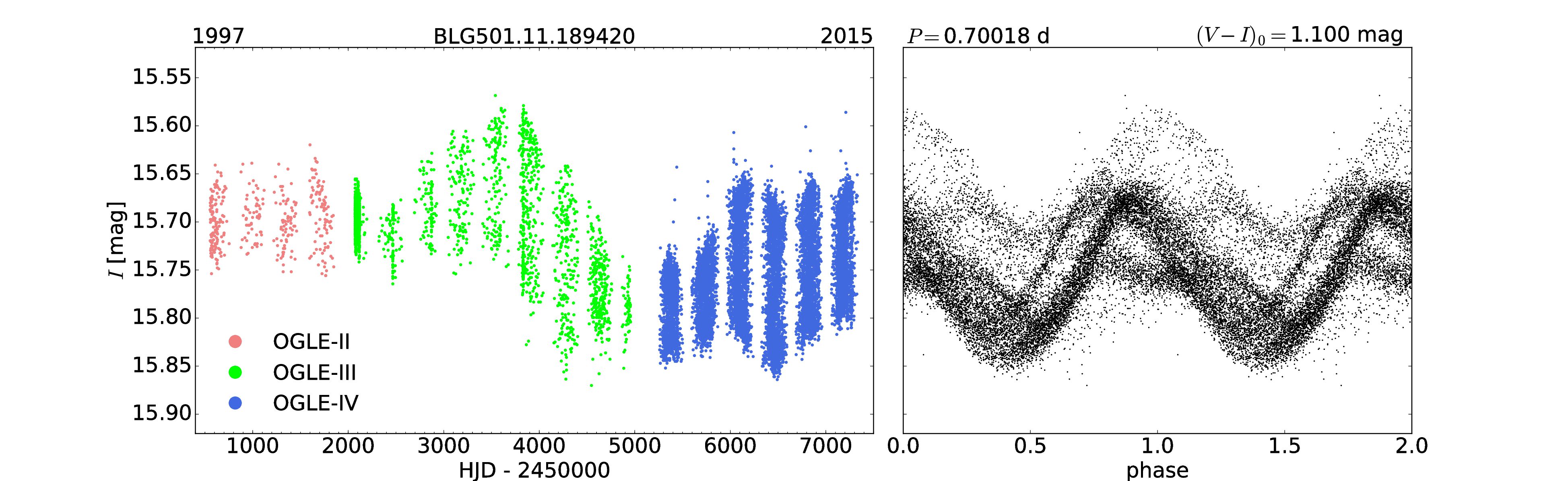
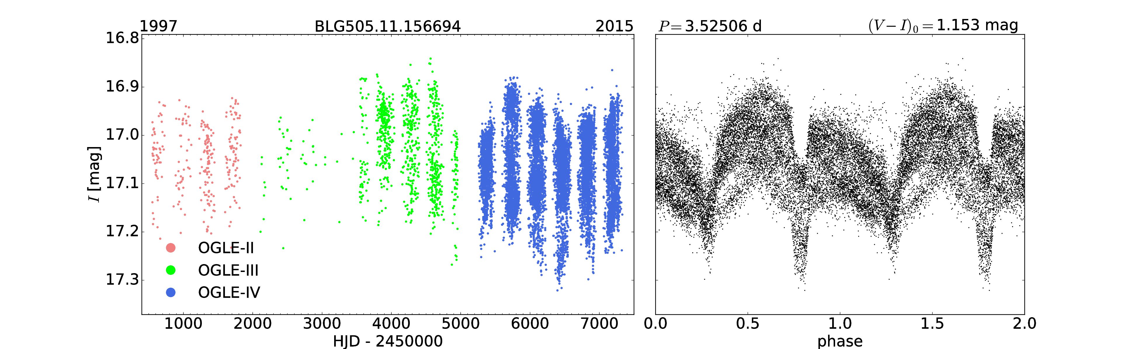
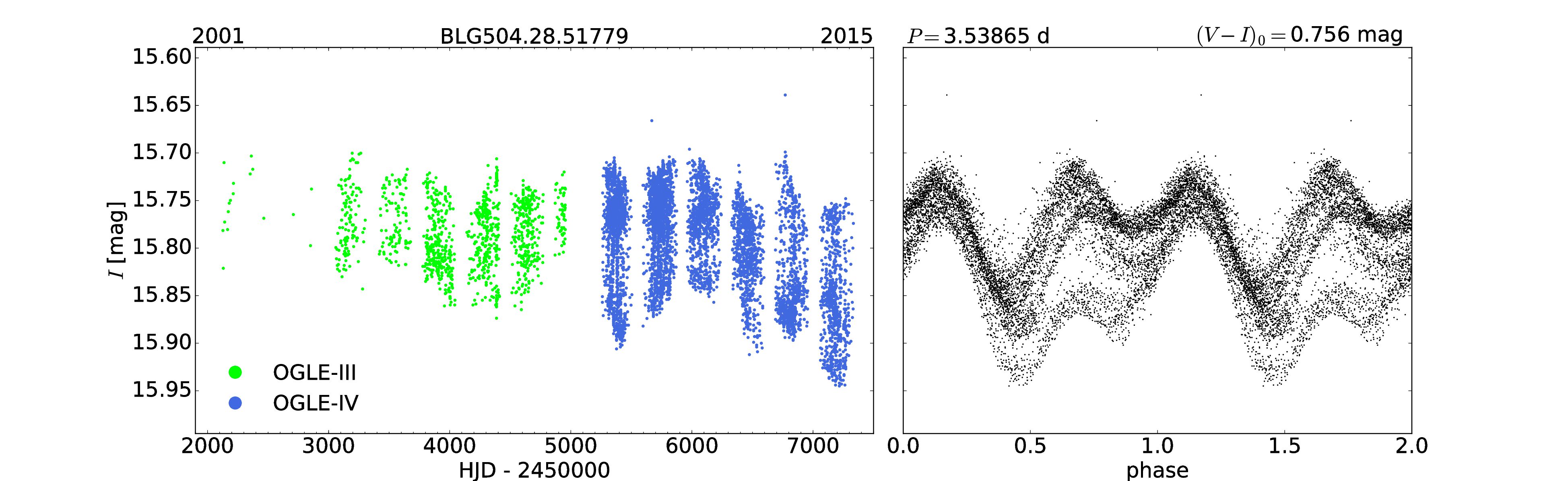
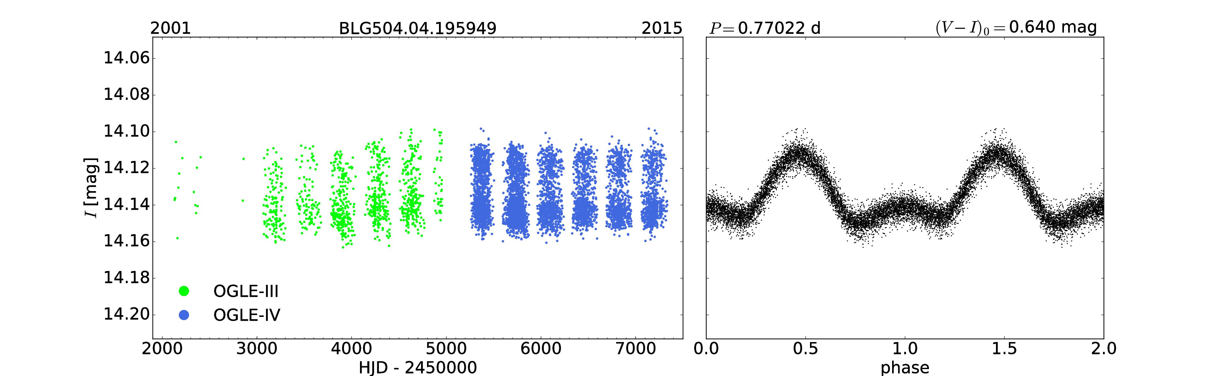
Figure 1.— Four examples of the spotted stars’ light curves from our collection. In the top row we can see a star with one dominant dark cool spot and no clear indication of binarity. In the second row, we can see a typical RS CVn-type eclipsing system. In the third row, we present a star with two dominant dark cool spots. The bottom row presents star with chemically peculiar spots. Left hand-side panels show unfolded light curves, while the right hand-side panels show phase-folded light curves with rotation periods $P$ (in the case of second plot we show the orbital period). The rotation period $P$ and color index $(V-I)_{0}$ corrected for the interstellar extinction are indicated above the plots. The dates at the top of the non-phased plot mark the year when the observations started, and the year of the last used observations. Individual phases of the OGLE project (OGLE-II, OGLE-III, and current OGLE-IV) are marked with different colors.

Examination of stellar spots and stellar activity is closely related to the study of mechanisms responsible for the generation of magnetic field in stars. The first model of magnetohydrodynamic dynamo was provided by Parker (1955). In this model, active regions of stars (including spots) arise as a result of ejecting a magnetic flux from deep layers of the convective zone onto the stars’ surface. Contemporary research has shown that rotation is a key in the generation of magnetic field of stars, and thus in the generation of phenomenon of stellar activity (Kraft, 1967; Skumanich, 1972; Durney and Latour, 1978). The examination of quasi-periodic brightness variations due to the magnetically active regions on stellar surfaces is closely related to the study of their rotation (e.g. Irwin et al. 2009). Stars with clear manifestations of the magnetic field activity are an excellent laboratory for testing dynamo models and a mine of knowledge about differential rotation (e.g. Guerrero et al. 2013, 2016a, 2016b, 2018). One of the largest samples of stellar rotation periods to date was published by McQuillan et al. (2014) from the Kepler space mission data and it consists of 34 030 records.

Another studies of the stellar activity showed a strong correlation between rotation periods and X-ray emission (Pallavicini et al., 1981), H$\alpha$ emission (Mekkaden, 1985), UV emission (Simon & Fekel, 1987), radio emission (Drake et al., 1989), and frequency of flares (Maehara et al., 2012).

The era of large-scale sky surveys initiated massive studies of stellar variability, including the variability caused by manifestation of the magnetic field. An extensive statistical analysis of spotted giants and subgiants, based on MACHO data (MAssive Compact Halo Objects, Alcock et al. 1995) was obtained by Drake (2006). Kiraga (2012) and Kiraga and Stępień (2013) analyzed over 2000 spotted stars based on the ASAS survey (Pojmański, 1997, 2002). Recently Lanzafame et al. (2018a, b) examined almost $150\;000$ late-type spotted dwarfs candidates found in the Gaia Data Release 2 (Gaia DR2; Gaia Collaboration 2016, 2018).

Here we present a detection and statistical analysis of $12\;660$ stars inside and toward the Galactic bulge found in the data collected by the OGLE project (Optical Gravitational Lensing Experiment; Udalski et al. 2015). As the Galactic bulge is one of the most challenging regions to explore in the Milky Way, because of the large and highly nonuniform interstellar extinction toward this direction, we propose here a new approach for the dereddening procedure. In the first part of this work, we try to verify correlations found by Drake (2006) and Lanzafame et al. (2018a, b). The second part of the paper is devoted to the two linear correlations between changes in brightness and changes in color that we discover for spotted stars. In the third part of this work, we conduct a basic analysis of stars with flares, which we find among all the spotted stars from our sample.

2. Observations

Long-term, high-cadence, multi-color, precise photometric observations play a key role in the analysis of stellar magnetic activity. For this reason, we use observations collected during three subsequent phases of the OGLE project: OGLE-II (1997–2000), OGLE-III (2001–2009), and OGLE-IV (2010–2015). Each phase marks the improvement in CCD camera size. The fourth phase of the OGLE project is still ongoing. However, for the purposes of this analysis, we use data collected by the end of the 2015. All data were obtained with the 1.3-meter Warsaw Telescope located at Las Campanas Observatory, Chile, which is operated by the Carnegie Institution for Science. During the OGLE-II phase about 30 million stars in the area of 11 square degrees in the central parts of the Milky Way were permanently monitored. In the next two phases, the sky coverage was extended, and now, during the OGLE-IV phase, we regularly observe more than 400 million stars in the area of 182 square degrees of the Galactic bulge.

During the ongoing OGLE-IV phase, a 32-detector mosaic CCD camera covering an area of about 1.4 square degrees in the sky is used. Observations are carried out in two standard I- and V-band filters of the Johnson-Cousins photometric system. Most of our observations are taken in the I-band with an exposure time of 100 s. The number of collected data points greatly varies between individual fields – for the most sampled fields we obtained over 13 000 data points and for the least sampled $\sim$100 data points. In the V-band, we have secured from several up to over 100 epochs per star with an integration time of 150 s.

All images collected by OGLE are reduced with the standard Difference Image Analysis (DIA) technique (Alard & Lupton, 1998; Woźniak, 2000). For more details about the OGLE instrumentation, data reductions, calibrations see Udalski et al. (2015). Details about the sky coverage and observing cadence can be also found on the OGLE website.

3. Selection and data sample

The majority of spotted stars in our collection have been found as a by-product of the massive search for eclipsing binary systems in the Galactic bulge (Soszyński et al., 2016), but many more have been found during searching for pulsating stars in the Milky Way (Udalski et al. 2018, Soszyński et al., in prep.). Periodic light curves with a characteristic long-term modulation of amplitudes and mean magnitudes were flagged as candidates for spotted variables. Typical long-term modulation of stellar brightness of spotted variables has time-scale of order of several years, and it is directly related to the magnetic activity cycles, similar to the Sun. In addition, strictly periodic stars (with no significant changes of the mean brightness) were also included (very likely candidates for CP stars). Each light curve in our sample has been visually inspected at least once, and usually a few times by more than one experienced astronomer. The light variability caused by stellar spots may be confused with semiregular variations due to radial and non-radial pulsations in red giant stars (long-period variables, e.g. Soszyński et al. 2013). However, in the most cases we were able to distinguish between both types of variable stars using their time-series photometry. As shown in Figure 1 of Soszyński et al. (2013), long-period variables change their amplitudes from cycle to cycle, while spotted variables exhibit much slower variability of the amplitudes. In most cases, the well-covered, long-term OGLE light curves allowed us to unambiguously separate spotted stars from pulsating variables. In total, we found over 20 000 candidates for spotted stars toward the Galactic bulge in the OGLE-IV database. From all of the spotted stars found in the OGLE-IV data, we have chosen 12 660 objects which were also observed during the OGLE-III phase because the interstellar extinction maps are available for these stars (Nataf et al., 2013). Stars observed only during the fourth phase of the OGLE project were not taken into account as the interstellar extinction is not yet available for them. The final sample contains stars with clear magnetic field manifestations, including classical dark spots, peculiar chemical spots or even flares. In Figure 1, we present examples of four light curves of spotted stars from our collection.

In Figure 2, we present a histogram of the apparent mean brightness of the spotted stars in the I- and V-band filters. It is important to note that beyond the maximum number of stars at $16.7$ mag in the I-band the number of objects decreases rapidly down to a limiting value of about $19.4$ mag, where no more stars with spots were detected. In the case of eclipsing binaries observed toward the Galactic bulge, the most common brightness value is about $18.4$ mag (Soszyński et al., 2016). Moreover, the OGLE photometry is complete and very accurate up to $18.7$-$19.5$ mag in the I passband (depending on the crowding; see Fig. 17 in Udalski et al. 2015). This may suggests that stars with strong magnetic activity are statistically brighter than stars that do not show such activity. However, we cannot rule out a possibility that this may be a selection effect as we did not calculate the detection efficiency neither for eclipsing nor for spotted stars. For the central regions of the Milky Way bulge the limit of brightness measurement of the Warsaw telescope is $I\approx 21$ mag (Udalski et al., 2015).

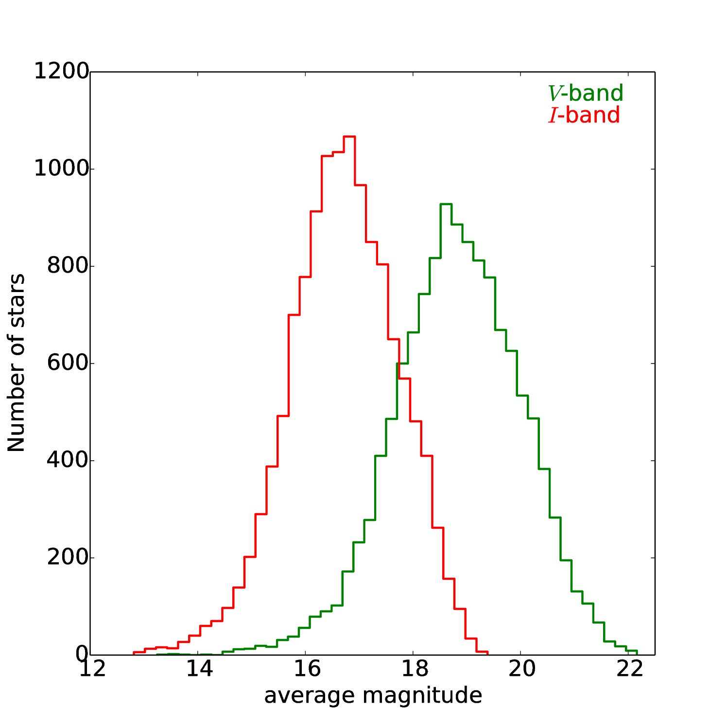
Figure 2.— Histogram of average brightness in I- and V-band for spotted stars.

4. Period searching

The methodology of looking for periodicity in time-series data is very complex and not trivial. There exists no fully automated method that would give periods at $100\%$ level of certainty. Therefore, our method of searching for periods is semi-automatic. This means, that we first calculate a periodogram for each star, from which we pick the most significant period based on the signal-to-noise ratio. In the second step, each light curve folded with that period has been carefully verified visually. If we decide that the found period is incorrect, it is corrected manually. This operation is repeated iteratively until a satisfying period is found. In the case when we are not able to find the reliable period, we exclude the star from further analysis.

In our analysis we use Fnpeaks code based on the standard Discrete Fourier Transform modified for unevenly spaced data (Kurtz, 1985). On the other hand, one of the most widely used period searching method in astronomy is Fourier-like least-squares spectral analysis proposed by Lomb (1976) and Scargle (1982). Recently, this method was discussed in great detail by VanderPlas (2018). Here we compare the results obtained from both methods.

Before computing the periodograms, we remove the long-term trends from the data using splines. Afterwards, for each star we compute high-resolution power spectra using both methods. We searched a frequency space from $0$ to $10$ d^-1, with a step of $0.000001$ d^-1. To compare the results from both methods we introduce three period symbols: $P_{\mathrm{FNN}}$ is the period obtained using Fnpeaks code, without visual inspection of light curves, $P_{\mathrm{FN}}$ is the period obtained using Fnpeaks code but adopted after visual verification and $P_{\mathrm{LS}}$ means period obtained with Lomb-Scargle algorithm.

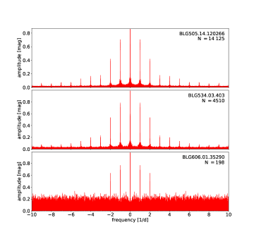
Figure 3.— Spectral window function for typical OGLE cadences: the most frequently observed field (top panel), the moderately covered field (middle panel) and the poorly covered field of our sample (bottom panel). By N we denote the number of observations for a given star.

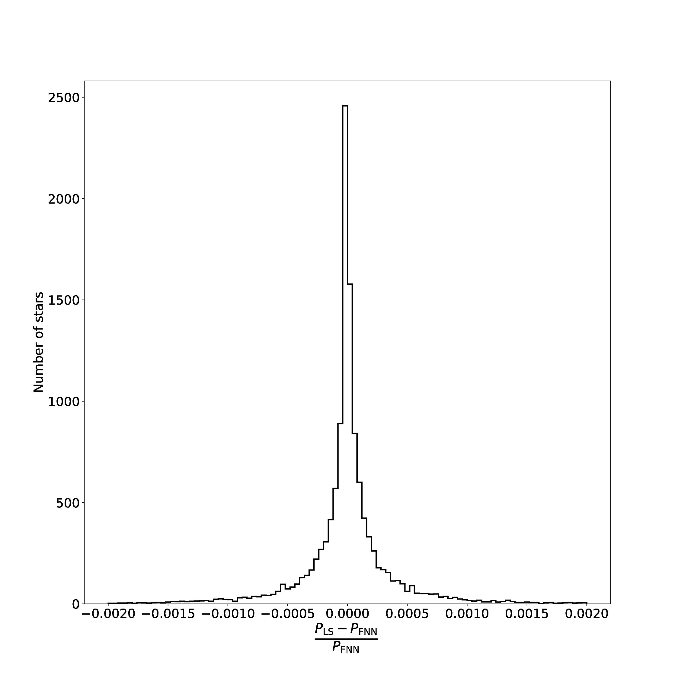
Figure 4.— Histogram of the relative differences between the periods obtained using different methods. $P_{\mathrm{LS}}$ means the period found using Lomb-Scargle algorithm, while $P_{\mathrm{FNN}}$ denotes the period found with Fnpeaks code without visual inspection.

Figure 5.— An example of a star, for which both period searching methods failed. The first panel presents the unfolded light curve. The next three panels show phase-folded light curves with the found rotation periods $P_{\mathrm{LS}}$ (second panel), $P_{\mathrm{FNN}}$ (third panel) and $P_{\mathrm{FN}}$ (fourth panel). The meaning of point colors and dates above the plot is the same as in Figure 1. Additionally, each phase-folded light curve is plotted with different colors related to different phases of the OGLE project. Above the fourth panel we also provide the color index $(V-I)_{0}$ corrected for the interstellar extinction.

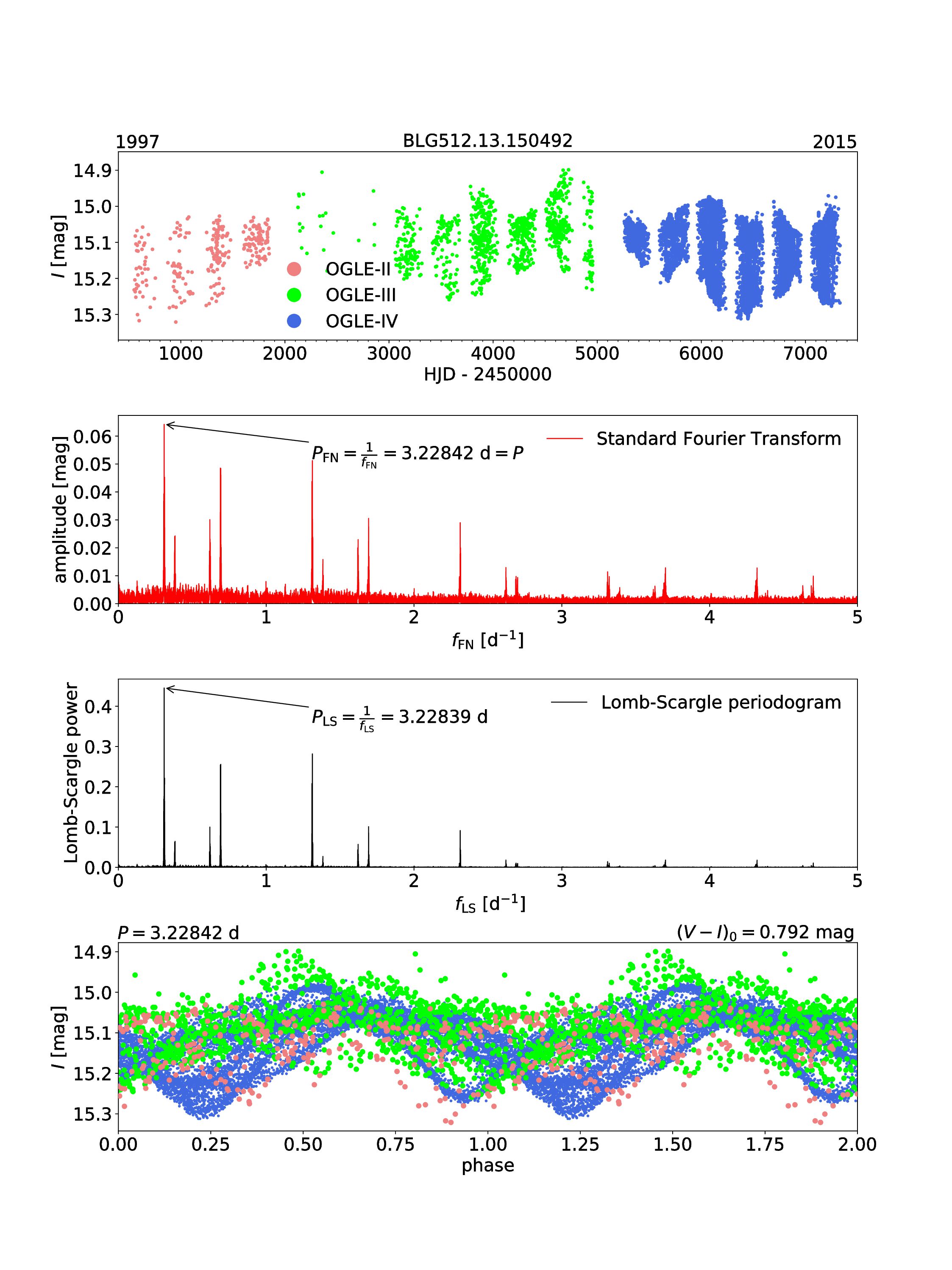
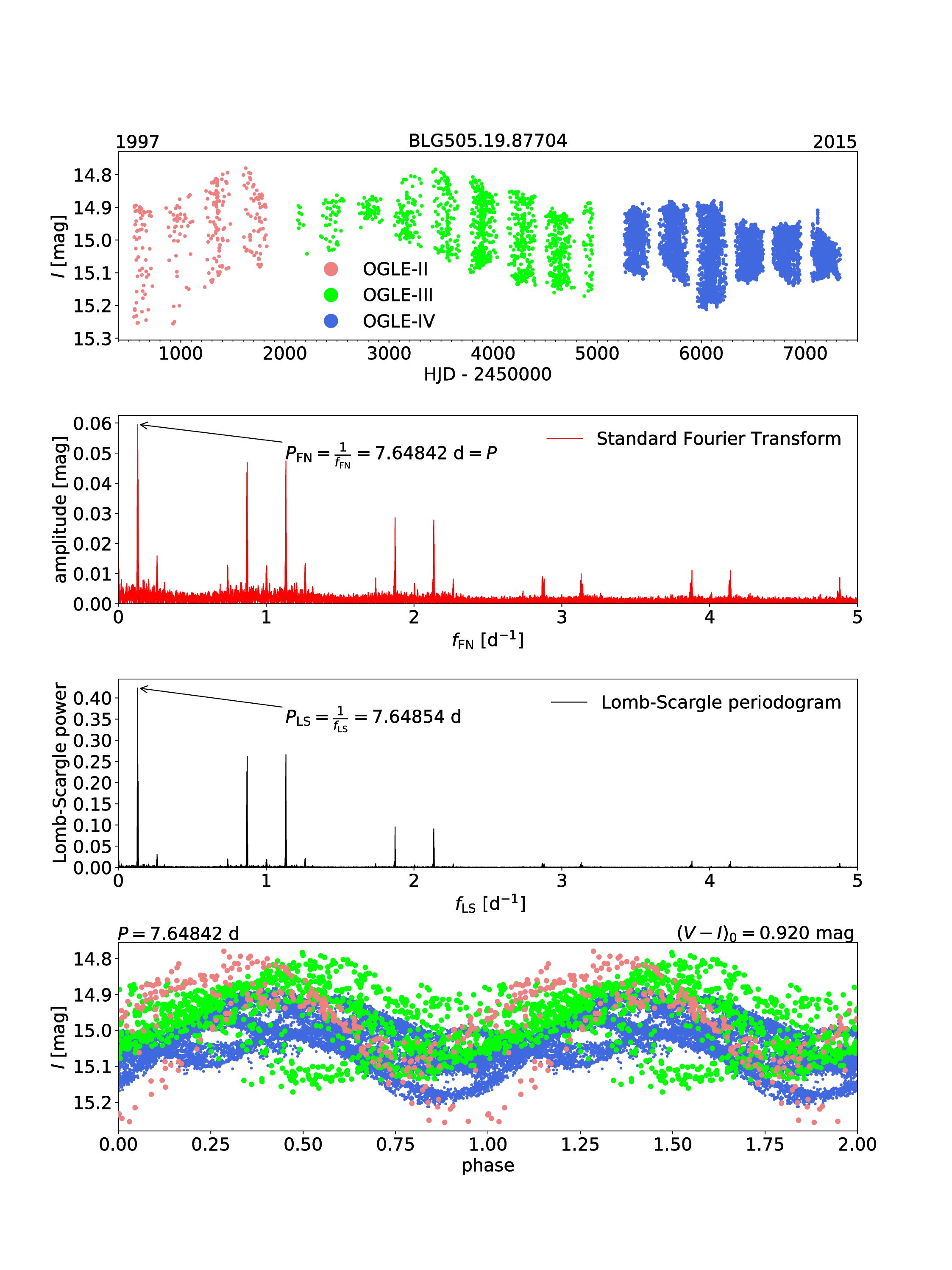
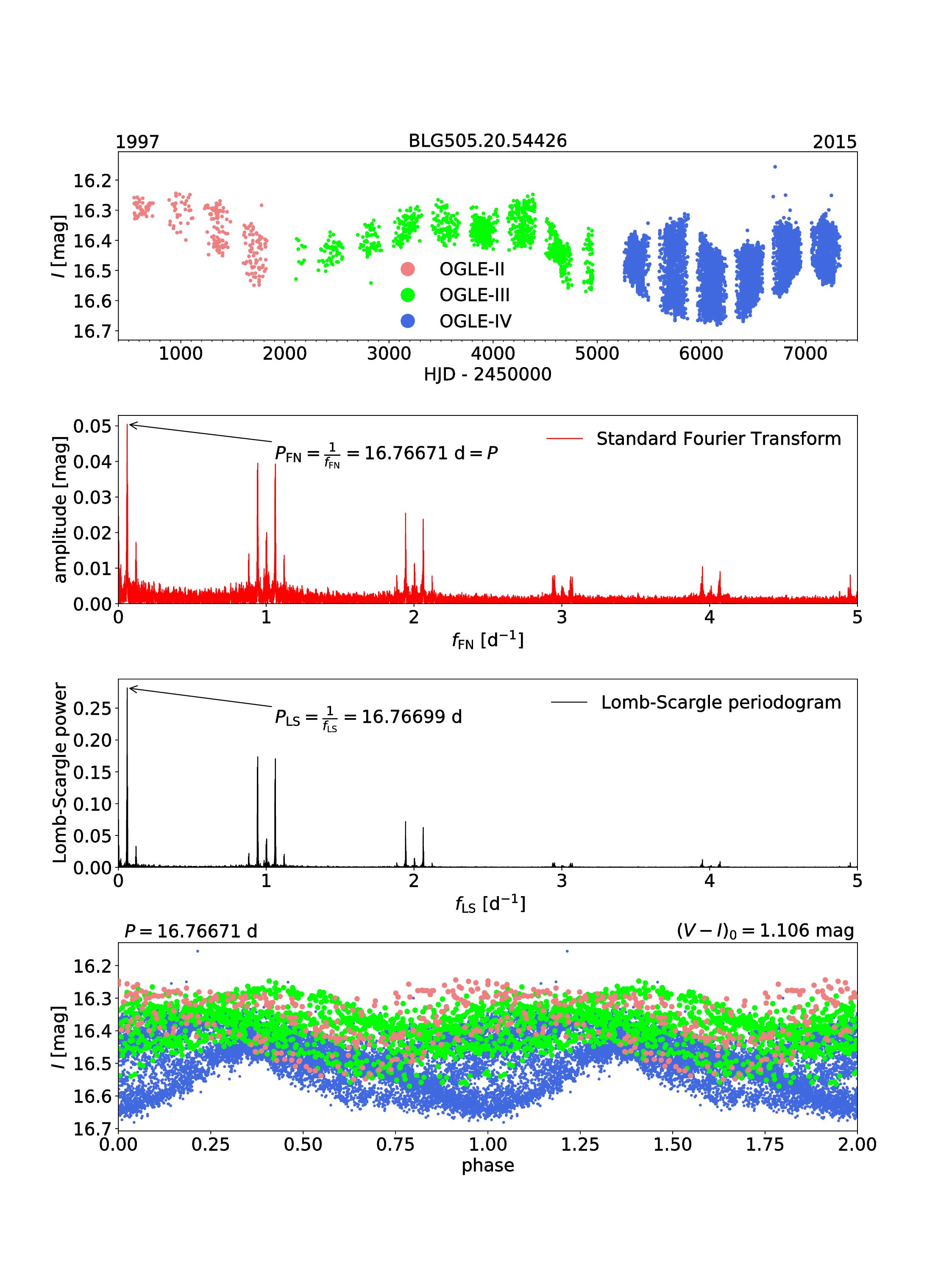
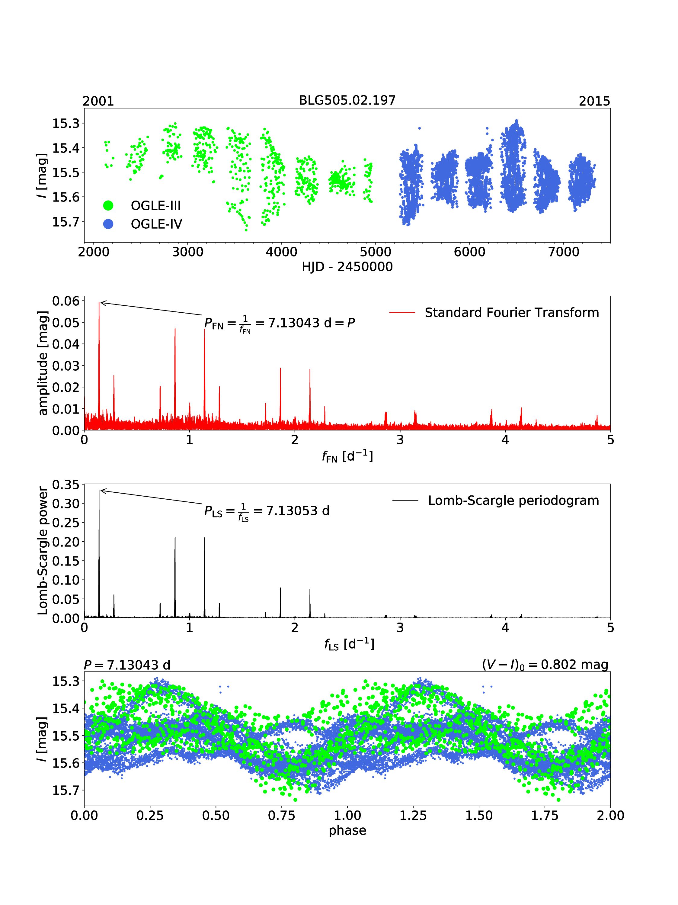
Figure 6.— Examples of four stars, which show a clearly visible, long-term (from months to years), quasi-periodic variability due to the evolution and migration of spots, and activity cycles. The first and last panels on each plot present time-domain and phase-folded light curves, respectively. The colors of points and dates above the panels have the same meaning as in Figure 1 and Figure 5. The second and third panels on each plot present typical periodogram patterns, which result from the stellar rotation combined with the more complex, quasi-periodic, long-term behavior. The periodograms on the second panels are obtained using Fnpeaks code, while the third panels show periodograms obtained using Lomb-Scargle algorithm. On each periodogram we marked the peak with the highest signal-to-noise ratio by an arrow, with appropriates period values following from the peak frequencies. Above the fourth panels we also provide color indices $(V-I)_{0}$ corrected for the interstellar extinction.

The OGLE Galactic bulge data (as other ground-based observations) are contaminated by two main aliases, $1$-day alias and $1$-year alias. In addition, the fields we observe have different cadences and coverages. The spectral window functions, and therefore typical aliasing structures arising from the OGLE cadences, are presented in Figure 3, separately for the most frequently observed field with the largest number of epochs (BLG505; top panel in Figure 3), moderately covered field (BLG534; middle panel in Figure 3, and poorly covered field (BLG606; bottom panel in Figure 3). It is clearly seen, that the choice of the period searching method may have a great importance for poorly covered light curves with a low cadence, because the noise level for them substantially increases. In such cases the Lomb-Scargle algorithm gains, because it reduces noise, as the noise is chi-square distributed under the null hypothesis (VanderPlas, 2018). However, it must be noted that our least covered light curves have less than $200$ epochs (only $6$ objects out of $12\;660$), while the vast majority of spotted stars have more than $500$ observations ($11\;790$ objects). More than a quarter of the objects have over $4000$ epochs, and nearly $2000$ of them have a light curve coverage at the level of more than $10\;000$ epochs.

In Figure 4, we present a comparison of periods calculated using both applied methods. We find that for $148$ stars the relative difference between found periods are higher than $1\%$. This difference is related to the fact that one of the methods reports $1/2$x or $2$x harmonics of real period, or one method reports the real period while the other reports a $1$-day alias. One example of this behavior can be seen in the light curves of the star BLG501.20.102890 presented in Figure 5. Please note, that in this case both methods give wrong periods. Thanks to the careful visual examination of the light curve, and manual correction ($P_{\mathrm{FNN}}$ period), it can be clearly seen that the star is a spotted eclipsing binary. On the other hand, in such binaries we expect to find at least two periods – one orbital, resulting from eclipses (if inclination is favorable), and the other, resulting from the rotation of the unevenly spotted primary component. We also expect that these two periods may be synchronized, or almost synchronized. Indeed, after substracting from the light curve the orbital period, it is possible to find a rotation period of the spotted primary star. This period was found by Lomb-Scargle algorithm and is presented in the second panel of Figure 5. Looking at the light curve in time-domain, one can see that a long-term modulation of the mean brightness and amplitude is visible due to activity cycle, which produces additional peaks in low frequencies. All these cases show that a visual inspection of the light curve is an indispensable method for examining in great detail the nature of a star, and all fully-automatic methods can fail for stars with such a complicated, fast-evolving variability.

For other stars from our sample the relative difference between the periods found from different methods is much smaller than $1\%$, with the average value at the level of accuracy of period searching methods. In general, there are $751$ object in our collection for which both methods give different periods by a factor of $1/2$ or $2$.

The amplitudes of brightness and the mean brightness of spotted stars vary rapidly in time due to the spots evolution and activity cycles. Typical time-scales of such changes are from months to several years. In Figure 6, we present four stars from our collection, with such a variability. Beside the light curves (in time-domain and phase-folded) we also show in Figure 6 typical power spectra resulting from stellar rotation combined with the more complex quasi-periodic, long-term brightness variations.

Both methods of period searching have advantages and disadvantages. However, thanks to the fact that our final method is not fully automated, there is a really small chance that some periods reported by us are not real. Of course, we cannot guarantee that each of the found period is perfectly correct. Nonetheless, we are convinced that the number of the misidentified periods is practically negligible and does not affect at all our statistical studies of spotted stars. In the further analysis we use periods found using Fnpeaks code $P_{\mathrm{FN}}$ and we name them $P$ throughout the paper.

In Figure 7, we present a histogram of rotation periods for the spotted variables from our collection. The shortest rotation period in our sample is 0.113 d and the longest one is 98.951 d. Such a large range of periods suggests that the presence of magnetic activity does not depend on the rotation velocity. However, the strength and form of the activity caused by the magnetic field may depend on how fast the star rotates.

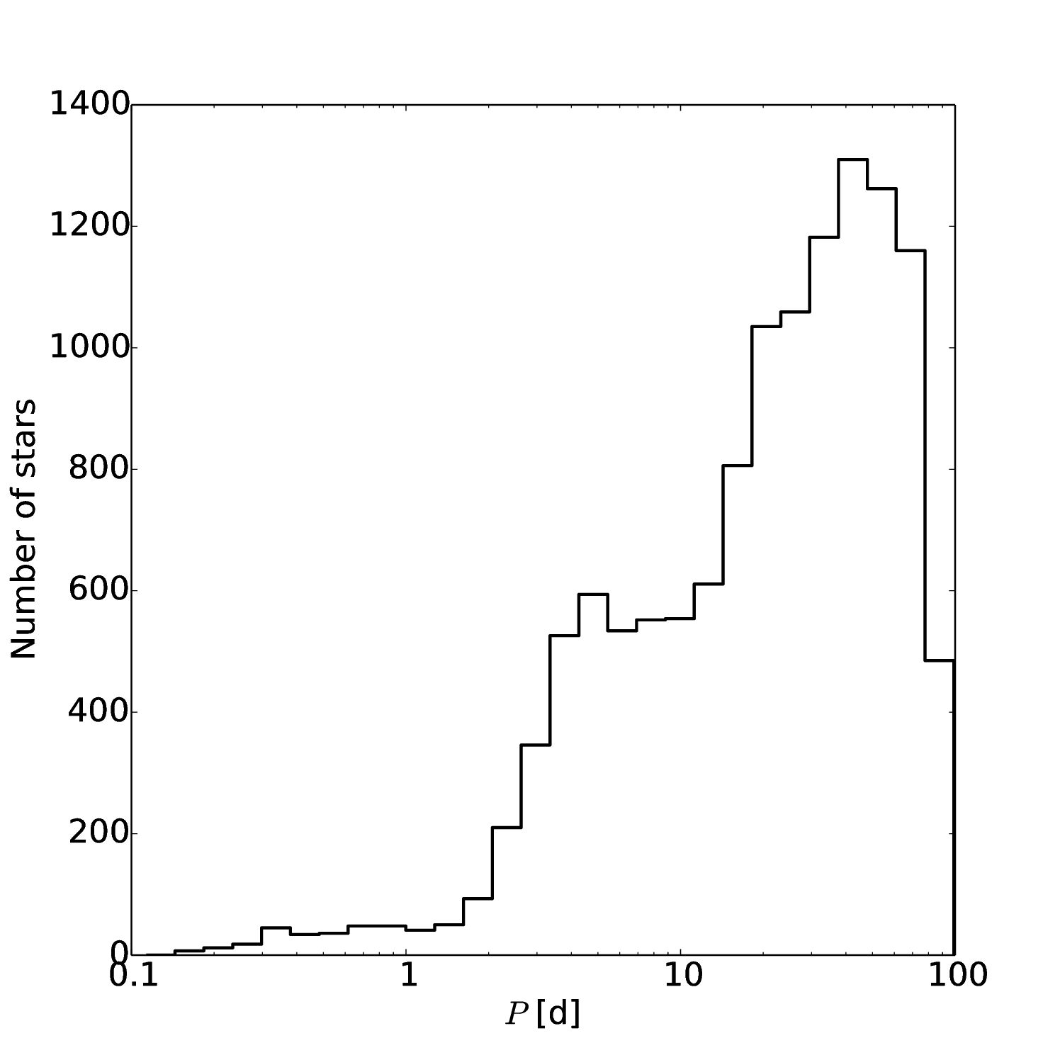
Figure 7.— Histogram of rotation periods of spotted stars.

5. Dereddening procedure for spotted stars

The Galactic bulge is one of the most challenging regions to explore in the Milky Way, as the light of stars observed in this direction is substantially and unevenly reddened due to irregular interstellar clouds of dust. Extinction and reddening can significantly change brightnesses and colors of stars on a small angular scale (see e.g. Udalski et al. 2002; Szymański et al. 2011). The OGLE observations are carried out mostly in the I-band. Observations in the V-band are much less frequent, but when we observe in the V-band, we usually obtain a corresponding I-band measurement just before or after frame in V bandpass. The majority of observations were made during the OGLE-IV phase, so for the color and mean brightness calculations we use the data just from this phase. The brightness of many spotted stars is rapidly changing, so we choose pairs of brightness measurements in both filters taken within 0.1 day and we calculate the observed color indices $(V-I)$. Typically, there are a few dozen of $(V-I)$ measurements per star, and this number corresponds to the number of measurements in the V-band. For every star, we calculate the median value of $(V-I)$ index and we reject all points deviating more than $\pm 3\sigma$ from the median. After removing outlying measurements we compute the $(V-I)$ median again.

For the majority of stars the extinction-free brightness $I_{0}$ and color index $(V-I)_{0}$ can be calculated with extinction $A_{I}$ and reddening $E(V-I)$ estimated from the colors of red clump stars by Nataf et al. (2013):

$$I_{0}=I-A_{I}\newline ,$$ (1)

$$(V-I)_{0}=(V-I)-E(V-I).$$ (2)

However, if we assume that the light from all stars experience total reddening and extinction observed toward the red clump stars in the bulge, we would certainly overestimate the dust influence on a fraction of the stars lying closer to us, in the Galactic disk. The results of dereddening using the interstellar extinction map made by Nataf et al. (2013), are presented in the left panel of Figure 8.

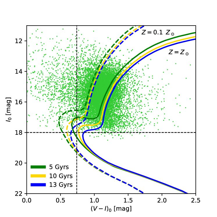
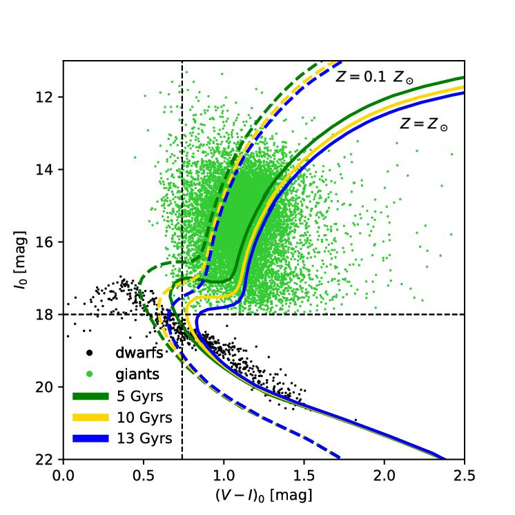
Figure 8.— Dereddened color–magnitude diagrams (CMD) for the analyzed spotted stars in our sample, marked with green dots. In both panels, we plot PARSEC isochrones (Bressan et al., 2012) for solar metallicity ($Z=Z_{\odot}=0.0196$; von Steiger & Zurbuchen 2016; marked with solid lines), and for $10\%$ of the solar metallicity (marked with dashed lines). With colors we marked three different ages of stars. Left panel: Dereddened CMD using $A_{I}$ and $E(V-I)$ calculated by Nataf et al. (2013). By dashed black lines we marked a region dominated by the foreground objects for which reddening is overestimated (top-left). The vertical dashed line is set at $(V-I)_{0}=0.74$ mag, what is the center of RGB region shifted by $2\sigma$ toward bluer colors (for RGB $(V-I)_{0}=1.10\pm 0.18$ mag). The horizontal dashed line presents the lowest brightness of giants located in the Galactic bugle, ${M_{I}}=3.5$ mag (distance modulus $\mu_{0}=14.5$ mag). Right panel: Dereddened CMD using our new method. Dashed vertical and horizontal lines have the same meaning as in the left panel. Green dots correspond to giants and black dots to dwarfs.

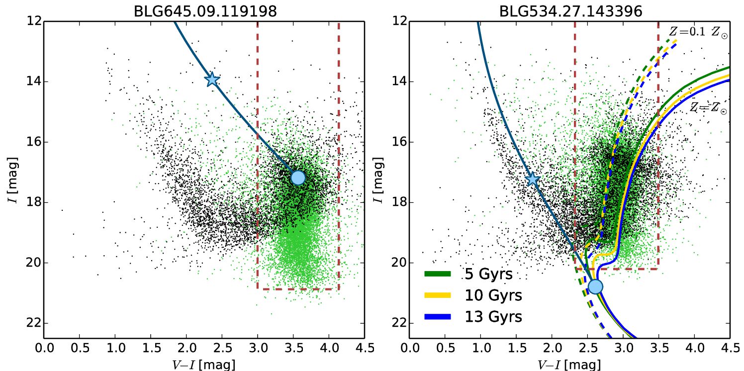
Figure 9.— Visualization of the dereddening procedure for two cases in the color–magnitude diagrams. Isochrones are plotted in the same manner as in Fig. 8. The blue star marks our analyzed spotted object. The solid blue line represents the reddening curve. The blue dot marks the star location after dereddening procedure. Green points show all the spotted stars from our sample. Black points mark a sample of stars from the neighborhood in the direction toward the analyzed object. Red dashed rectangle presents RGB region defined by $(V-I)_{0}=1.10\pm 2\sigma\pm\sigma E(V-I)$, $M_{I}<3.5$ mag. Left panel: A case when the spotted star is clearly a foreground giant. In this case we set the color index for this star at $(V-I)_{0}=1.10$ mag and the brightness $I_{0}$ as it appears from the reddening curve. Right panel: A case when the spotted star is a dwarf. In this case we estimate $(V-I)_{0}$ and $I_{0}$ from isochrones. It is worth mentioning, however, that both $I_{0}$ and $(V-I)_{0}$, adopted for dwarfs are very uncertain.

The majority of analyzed stars fall into the Red Giant Branch (RGB) region. We can describe this region in the color–magnitude diagram (CMD) by the average color index $(V-I)_{0}=1.10\pm 0.18$ mag and the absolute magnitude $M_{I}<3.5$ mag. We assume that stars lying within the RGB region are in fact giants from the Galactic bulge, and that their reddening is as resulting from the interstellar extinction map presented by Nataf et al. (2013). Stars that appear bluer might be foreground giants or dwarf stars, and the amount of reddening toward them should be smaller than calculated according to Nataf et al. (2013) for a given line of sight. We assume that all stars bluer than $2\sigma$ from the typical RGB color $(V-I)_{0}=1.10$ mag, i.e. bluer than $(V-I)_{0}=0.74$ mag (vertical dashed line in both panels of Fig. 8), are potential foreground objects (objects located in the top-left part of the CMDs in Fig. 8). In fields with large differential reddening we shift this boundary by $\sigma E(V-I)$ as calculated by Nataf et al. (2013).

We simulate extinction between the Sun and the analyzed spotted star assuming that the extinction is proportional to the dust density $\rho_{\mathrm{dust}}$, which can be modeled by a double exponential disk:

$$\rho_{\mathrm{dust}}\propto\exp\left(-\frac{R-R_{0}}{h_{R}}\right)\exp\left(-\frac{|z|}{h_{z}}\right),$$ (3)

where $R$ is distance from the Sun to the analyzed star, $R_{0}$ is distance from the Sun to the Galactic bulge and $z$ is vertical distance of the analyzed object from the Galactic plane. We use the length and height scales ($h_{R}$ and $h_{z}$, respectively) as calculated by Sharma et al. (2011) with values $h_{R}=4200$ pc and $h_{z}=88$ pc. These parameters were found by the authors using Schlegel et al. (1998) dust maps in the Milky Way. We normalize the dust density $\rho_{\mathrm{dust}}$ measured in the given direction to the total reddening as measured by Nataf et al. (2013).

Using the above extinction model, we are able to spread out the entire reddening $E(V-I)$ along the line of sight toward the star with unknown reddening. This allows us to move the star along the reddening curve and estimate what brightness and color it would have, if it were located in the bulge. With this procedure, we can assess if this is a foreground giant or rather a dwarf star.

To decide whether the star could be a foreground giant, we take the least luminous RGB star from the Galactic bulge and shifts this object along the reddening curve toward us. If the observed star is more luminous than the shifted RGB bulge star we assign to this star $(V-I)_{0}=\leavevmode\nobreak\ 1.10$ mag and brightness $I_{0}$ according to the reddening curve.

Otherwise, the analyzed star must be a foreground dwarf. We can estimate the dwarf color and brightness based on the isochrones limited to the Main Sequence (MS) stage, where dwarfs spend the majority of their lives. We use PARSEC isochrones (Bressan et al., 2012) for the solar metallicity $Z=Z_{\odot}=0.0196$; (von Steiger & Zurbuchen, 2016), but see Serenelli et al. (2016), $10\%$ of the solar metallicity and for three ages: 5 Gyrs, 10 Gyrs, and 13 Gyrs. We place these isochrones in the bulge, and we shift them along the reddening curve toward the observer until they cross the star’s position on the CMD. The coordinates of this intersection are our searched extinction-free brightness and color for the analyzed dwarf. However, it is worth mentioning that this approach is affected by large uncertainties and only allows us to state if the star is indeed a dwarf.

We crossmatched our list of the spotted stars with general catalog of all sources published by Gaia Collaboration (2016; 2018) in the Data Release 2 using angular radius equal to 0.4 arcsec. We found, that $11\;915$ out of $12\;660$ objects from our list have measurements in the Gaia database. Unfortunately, only $24$ stars have significant parallaxes with $\sigma_{\varpi}/{\varpi}<0.05$, $108$ sources have measured parallaxes with $\sigma_{\varpi}/{\varpi}<0.1$, and $1465$ objects have parallax measurements with $\sigma_{\varpi}/{\varpi}<0.33$. This means that some stars from our sample are certainly located closer than the Galactic bulge. A fair fraction of objects found in the Gaia catalog have no parallax measurements, or have negative parallaxes ($5296$ stars), and the remaining objects from our list have insignificant parallax entries in the Gaia database.

The right panel of Figure 8 shows CMD after applying our new dereddening method. This approach allows us to classify $676$ stars as dwarfs, and $11\;984$ objects as giants. Two cases of our dereddening approach discussed above are presented in Figure 9. It is noteworthy, however, that while this dereddening procedure is acceptable for statistical analysis of large sample of stars, it may overestimate brightness and color of individual objects. This can be especially important for stars observed toward directions where high inhomogeneities of the interstellar dust distribution occur.

6. General properties of spotted stars

Two largest, up-to-date, statistical analyzes of spotted stars were obtained by Drake (2006), who discussed the properties of $\leavevmode\nobreak\ 3000$ giants and subgiants toward the Galactic bulge and Lanzafame et al. (2018b), who analyzed $\leavevmode\nobreak\ 150\;000$ BY Dra candidates detected in the Gaia DR2 data. In the present paper, we conduct a similar analysis as Drake (2006) but based on more than four times larger sample. A significantly larger set of examined stars and the long-term OGLE photometry allow us to examine more precisely correlations presented by Drake (2006) and to find new, previously unknown dependencies.

Below we discuss statistical properties of spotted stars. In most of the diagrams presented in this work we bin stellar parameters along x-axis. Usually, we calculate the mean values in each bin along the x-axis, and the median values along the y-axis. Diagrams with rotation periods are presented in a logarithmic scale. For the binning along the rotation periods, we require at least 50 points in each bin and a bin width of at least $\log{(P)}\leavevmode\nobreak\ =\leavevmode\nobreak\ 0.1$ dex. For the binning along the amplitudes we also require at least 50 points, but the width of the bins was $0.02$ mag. We mark these averaged values by large purple dots with appropriate error bars. Typically, error bars are smaller than, or equal to the size of the used symbols.

6.1. Location of spotted stars in the sky

In Figure 10, we present the location of analyzed spotted stars in the sky. The black contours show the outline of combined OGLE-II, OGLE-III and OGLE-IV fields toward the Galactic bulge. The Galactic bulge area is dominated by giants, which fill almost the whole area observed by OGLE. The great majority of these stars is located in the bulge itself. However some of them are, very likely, foreground Galactic disk objects. The central region of the Galaxy is impossible to observe in the optical range due to huge interstellar extinction in this part of the Milky Way, hence there is a lack of detections near the plane.

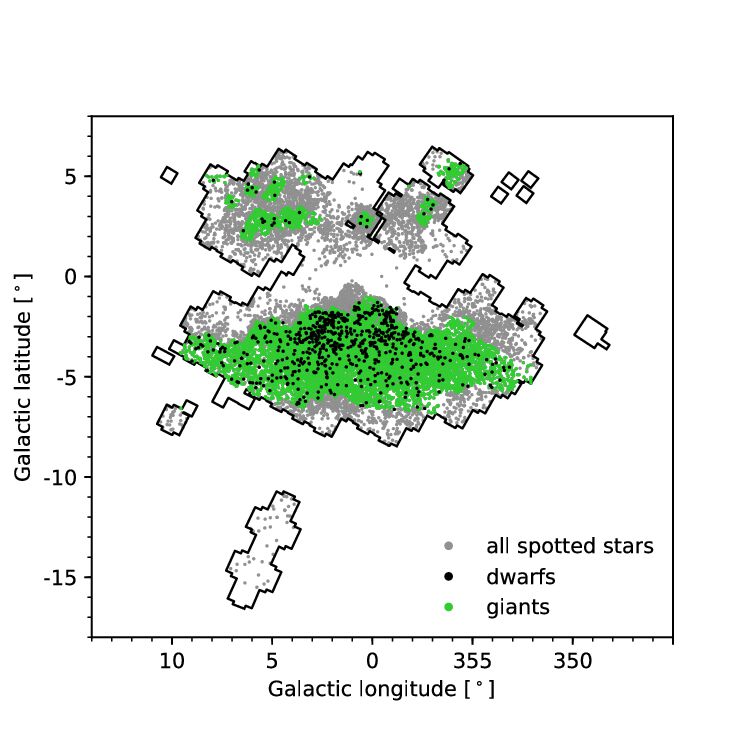
Figure 10.— Distribution of spotted stars in the sky toward the Galactic bulge. Black contours correspond to the OGLE footprint. Gray points denote all spotted stars discovered in the OGLE-IV data. Black and green points denote all stars analyzed in this paper coinciding with OGLE-III footprint. With green points we marked stars classified as giants, while black dots present objects classified as dwarfs.

6.2. I-band amplitude vs. rotation period – the final division into dwarfs and giants

The amplitudes of light curves of active stars vary significantly with time as a result of spots evolution. These variations are evident in the phased light curves presented in Figure 1. Therefore, before determining the average amplitudes over the time span of the OGLE project, we removed outlying measurements deviating more than $\pm 4\sigma$ from the mean brightness. A common approach to determination of the amplitude of brightness variations assumes fitting the Fourier series to the phased light curves. However, our tests show that this approach may produce spurious results for stars with a quickly changing average brightness. Using a second-order Fourier series, we find amplitudes of many light curves overestimated or underestimated. Similar results are obtained for higher or lower orders of the Fourier series. For this reason, we propose here another method of measuring amplitudes, which is free of the influence of average brightness variations.

We first transform each light curve into bins containing at least $200$ measurements and covering at least $5$ cycles of rotation. Mathur et al. (2014) found that the length of the bins equal to $5$ rotation cycles is optimal for active stars. In the next step we calculate for each bin the difference between $95$th percentile and the $5$th percentile of I-band magnitudes. This approach is similar to the activity proxy $R_{\mathrm{var}}$ defined by Basri et al. (2011, 2013) for Kepler stars. The final amplitude is defined as a median of all measurements divided by the distance between these two percentiles, i.e. $0.9$.

In Figure 11, we present amplitude-period plane for spotted stars from our sample. We notice that the investigated variables can be divided into two broad groups, depending on the rotation rate, and the amplitude of the brightness variations. The first one contains fast rotators ($P\leq 2$ d) with most of the amplitudes lower than $0.2$ mag and the second group contains slow rotators with periods up to $100$ d and amplitudes up to $0.8$ mag.

Our dereddening procedure revealed that $59\%$ stars (243 out of 415 objects) with rotation periods $P\leq 2$ d are very likely dwarfs. The remaining 172 stars from this group were flagged as probable giants, yet it is commonly known that giants cannot rotate so fast because they would be torn apart by the centrifugal force. We conclude that all stars with rotation periods shorter than 2 days, should be considered as dwarfs. This can be easily verified by calculating the critical rotation period $P_{\mathrm{crit}}$ for which a star would be torn apart by the centrifugal force. Using the Single Star Evolution code (SSE, Hurley et al. 2000) we calculate the evolutionary tracks for stars with masses on the Zero Age Main Sequence (ZAMS) in the range $1\leq M/M_{\odot}\leq 3$ with a step of $0.25$ $M_{\odot}$. We assume the solar metallicity ($Z=Z_{\odot}=0.0196$; von Steiger & Zurbuchen 2016) and the evolution time $T_{\mathrm{evolv}}=12$ Gyrs. We calculate the radius during the first third of the time spent by the star on the RGB, when the radius grows steadily, weighted by the time of evolution. In addition, we neglect any mass loss. Then we calculate the critical periods $P_{\mathrm{crit}}$ using equation 2 from Ceillier et al. (2017):

$$P_{\mathrm{crit}}=\sqrt{\frac{27\pi^{2}R_{\star}^{3}}{2GM_{\star}}},$$ (4)

where $R_{\star}$ and $M_{\star}$ are the radius and mass of the star and $G$ is the gravitational constant. After inserting solar units ($R_{\odot}$ and $M_{\odot}$) we obtain the following formula for the critical rotation period in days:

$$P_{\mathrm{crit}}=0.213\hskip 2.84544pt{\mathrm{d}}\hskip 2.84544pt\cdot\left(\frac{R_{\star}}{R_{\odot}}\right)^{\frac{3}{2}}\left(\frac{M_{\star}}{M_{\odot}}\right)^{-\frac{1}{2}}.$$ (5)

The resulting critical period for a one solar mass star is equal to $P_{\mathrm{crit}}=0.81$ d, for a two solar mass star it is equal to $P_{\mathrm{crit}}=2.97$ d, and for a three solar mass star it is equal to $P_{\mathrm{crit}}=8.92$ d. We see that the rotation periods around 2 days of the $172$ apparent giants are close to, or even shorter than their critical periods. This is why we assume that all the objects with periods $P\leq 2$ d, are dwarfs. Accordingly, the final number of dwarfs increased to $848$ objects, while the final number of giants is $11\;812$.

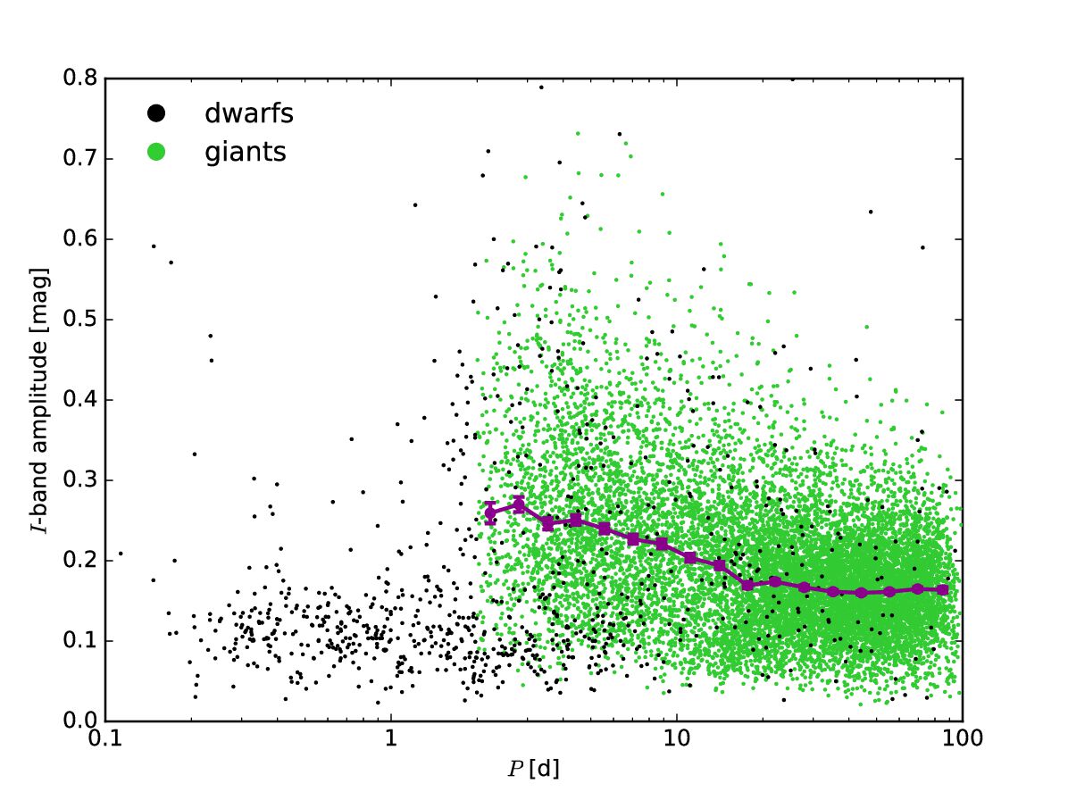
Figure 11.— I-band amplitude vs. rotation period $P$. The large purple points with error bars indicate the medians of I-band amplitude binned in $\log{(P)}$.

Summarizing Figure 11, the small-amplitude, fast-rotating group contains dwarfs, while the group with longer rotation periods having in many cases stars with amplitudes larger than $0.2$ mag contains dwarfs as well as giants with the vast majority of the latter.

Apart from fast-rotating, small-amplitude dwarfs, we also detect dwarfs with high amplitudes, but they are definitely slow rotators. We do not find any significant correlation between the amplitude and rotation period for dwarfs. However, for spotted giants we observe a clear correlation – the slower the giants rotate, the smaller amplitudes they have. It is noteworthy that, on average, slowly rotating stars exhibit larger secular brightness changes. This effect can be related to the mechanism responsible for generating stellar magnetic fields and thus starspots. It seems that slowly rotating stars have larger and slower evolving spots on their surfaces. However, it should be kept in mind that large amplitudes result from an asymmetry in the spotted area. Stars covered by spots evenly give a minimal, or just imperceptible change of luminosity. In the case of uniformly spotted stars, the amplitude in the optical band is insignificant, although the star can be very active. In such stars the activity level can be measured from the emission cores in the spectral lines CaII H and K (Baliunas et al., 1995) or X-ray flux (Pallavicini et al., 1981).

The extensive studies of spotted dwarfs from Kepler data showed that photometric variability is correlated with the rotation period. For instance, McQuillan et al. (2014) using variability index $R_{\mathrm{var}}$ defined by Basri et al. (2011, 2013) found, that higher amplitudes are observed in stars with shorter rotation periods. Similar picture for fast-rotating seismic solar analogs was obtained by Salabert et al. (2016) who used $S_{\mathrm{ph}}$ (Mathur et al., 2014) variability index. Recently, Lanzafame et al. (2018a, b) demonstrated the existence of bimodality in amplitude-period plane. The authors pointed out, that the fastest rotating dwarfs concentrate in two regimes of amplitudes – low and high, whereas the slowly rotating dwarfs show preferentially low photometric variability. Lanzafame et al. (2018a, b) concluded, that such a multimodality suggests the existence of different regimes of surface inhomogeneities in young, and middle-age stars. Our data partially confirm the above results for dwarfs. However, we do not see bimodality of amplitudes for fast rotators but it should be mentioned that amplitudes measured in our work are on average ten times larger. This is obviously related to the capabilities of the instrument – much lower amplitudes can be detected from the outer space compared to the ground-based instruments. Additionally, amplitudes may vary significantly depending on the filters in which an object is observed. On the other hand, amplitude measurements based only on the Gaia data may not be very accurate due to the low number of epochs. As we mentioned before, amplitudes of brightness of the spotted stars change rapidly. It is interesting, however, to see that our giants behave similarly to the slowly rotating dwarfs on the amplitude-period diagram, i. e. their amplitude decreases with the increasing period. Separation for both groups of stars, dwarfs and giants, is also visible around the rotation period $P\approx 2$ d.

6.3. Spatial distribution of the rotation periods

In Figure 12, we present a relationship between absolute values of Galactic latitudes and rotation periods of spotted stars from our sample. The most central region of the Milky Way is inaccessible for the OGLE observations, because the clouds of dust toward this region absorb the bulk of the light in the visual domain. Thus, there are no points with $|b|<1^{\circ}$ in Figure 12.

Drake (2006) noted that chromospherically active giants located close to the Galactic plane, have on average longer rotation periods. This correlation is indeed visible in Fig. 12 where the slow rotating giants are on average closer to the Galactic plane, but it is absent for dwarfs. We think, however, that the existence of this correlation for giants, and its lack for dwarfs is caused by the selection effect against shorter-period red stars with typically fainter V-band magnitudes which are missing in the sample close to the Galactic plane where the extinction is higher. In addition, stars with no detection in the V-band are missing by definition in our sample.

As mentioned before, the dereddened luminosities and colors for dwarfs are burdened with large uncertainties so we are left with rotation periods, variability amplitudes and Galactic coordinates as the only certain parameters for these stars. This is why we drop dwarfs from further analysis.

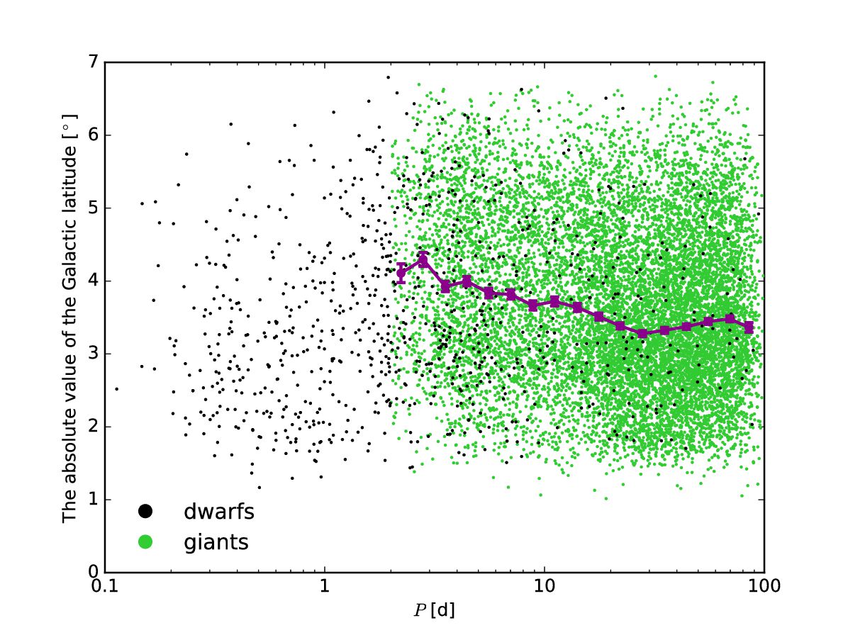
Figure 12.— Absolute values of the Galactic latitude $|b|$ vs. rotation period $P$ for the spotted variables. Large purple points with error bars indicate the median $|b|$ values binned in $\log{(P)}$.

6.4. $(V-I)_{0}$ vs. the rotation period

Drake (2006) found that the rotation period increases with color for stars with periods $P\lesssim 30$ d. In Figure 13, we present the dereddened color index $(V-I)_{0}$ as a function of the rotation period $P$ for stars from our sample. In the inset of Figure 13, we show a similar color range to that presented by Drake (2006). In both plots solid black lines are plotted at the median of $(V-I)_{0}$.

We cannot unambiguously confirm that this correlation exists by looking at a four times larger data set which covers substantially wider range of colors than the range presented by Drake (2006, see Fig. 14 therein). However, using a similar range as in Drake (2006) with the linear binning, this correlation can be marginally detected.

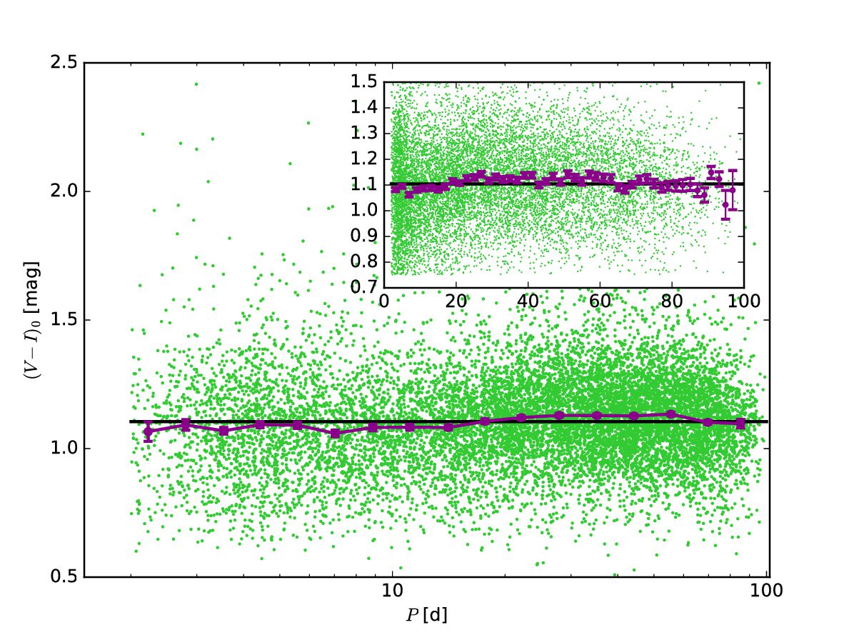
Figure 13.— Dereddened color index $(V-I)_{0}$ vs. rotation period $P$. Large purple points with error bars indicate the median $(V-I)_{0}$ values binned in $\log{(P)}$. Inset ranges correspond to Fig. 14 of Drake (2006). Here large purple points with error bars denote the median $(V-I)_{0}$ values binned in linear scale. Black solid lines represent the median values of the $(V-I)_{0}$. over the whole range of $P$.

6.5. $I_{0}$ vs. the rotation period

Previous studies of spotted, magnetically active stars have excluded the existence of a dependence between the brightness of the stars and the rotation period (Drake, 2006). In Figure 14, we present a plot of the extinction-corrected magnitude $I_{0}$ versus the rotation period $P$ for our giants.

We see a clear correlation between the brightness and period, such that the spotted giants are brighter when they rotate slower. The correlation is visible for stars with rotation periods of up to $50$ days and flatten for $P>50$ d. A range of rotation periods $50<P<100$ d contains $2630$ stars, while a range $2<P\leq 50$ d contains $9081$ stars. Perhaps the future detections of very slowly rotating giants will reveal the extension of this correlation.

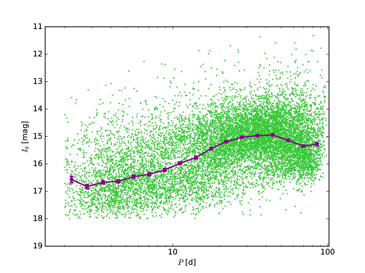
Figure 14.— Mean extinction-corrected I-band magnitude ($I_{0}$) vs. rotation period $P$. Large purple points with error bars indicate the median $I_{0}$ binned in $\log{(P)}$.

6.6. $I_{0}$ vs. the I-band amplitude

Drake’s (2006) study of chromospherically active stars showed the existence of a weak correlation between stellar brightness and variability amplitude. The author pointed out that faint stars exhibit larger brightness variations. In Figure 15, we present the relationship between the extinction corrected I-band magnitude $I_{0}$ and the I-band amplitude. The amplitudes are calculated in the same way as in Section 6.2.

In Figure 15, the correlation discussed in Drake (2006) can be clearly seen – the fainter stars have a stronger manifestation of the magnetic activity (i.e. larger spot coverage) and thus have larger amplitudes. Unfortunately, in our opinion an accurate examination of this correlation is almost impossible due to a selection effect – faint stars with small amplitudes are less likely to be detected and properly classified as spotted variables, so we do not expect to have many faint, low-amplitude objects in our collection. However, we found an interesting property of bright stars with $I_{0}\leavevmode\nobreak\ \lesssim 16$ mag. Save for a few exceptions, they do not exhibit amplitudes higher than $0.4$ mag. There is no any obvious selection effect which could produce this feature, so we believe that this finding is related to the nature of spotted stars. More detailed studies are needed for clarification of this phenomenon.

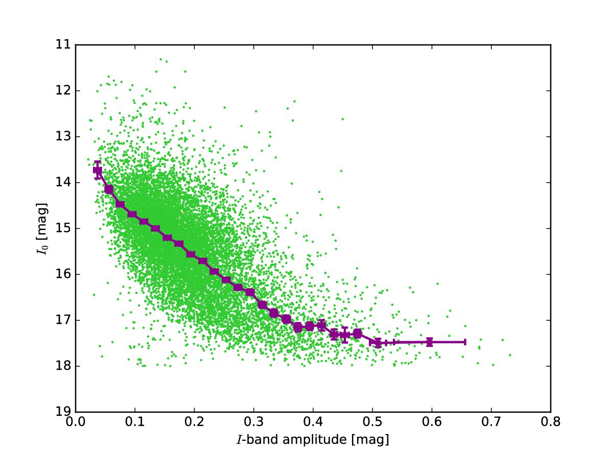
Figure 15.— Mean extinction-corrected I-band magnitude ($I_{0}$) vs. I-band amplitude. Large purple points with error bars indicate the median $I_{0}$ binned in I-band amplitude.

7. Two types of spots

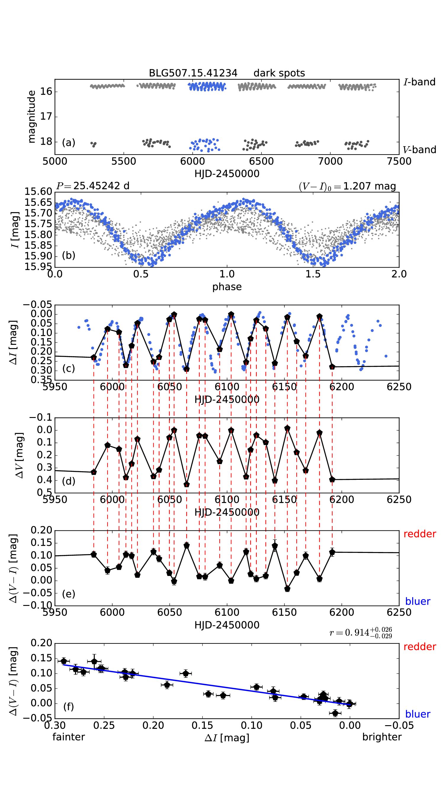
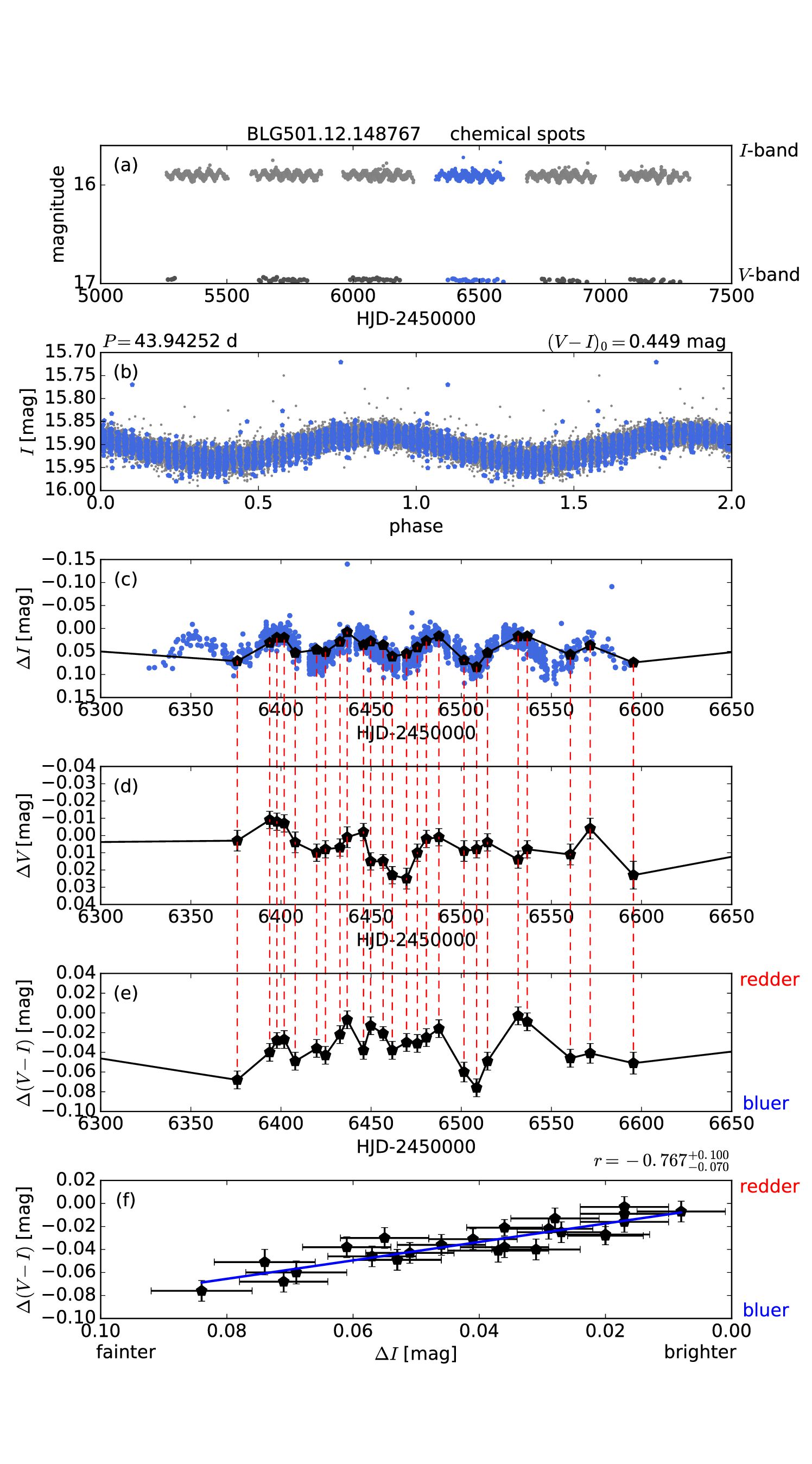
Figure 16.— Examples of different types of spots in two stars. The left panel shows an example of a star with dark spots (BLG507.15.41234), while the right panel shows an example of a star with chemical spots (BLG501.12.148767). (a) Whole light curves in both I- and V-band. Blue points denote observations analyzed on further plots. (b) Phase folded light curves with rotation periods given above each plot. Above the plot we also give dereddened color index $(V-I)_{0}$. (c) Changes in the I band for the time-span marked with the blue points in the top plots. Black points show measurements for which we have simultaneous I- and V-band observations. (d) Changes in the V band. (e) Color changes. (f) Correlations between color variations and brightness variations. The correlation coefficient calculated within the considered time range is given above the plot. For better visibility of these correlations we fitted straight lines to the data. All black points are plotted with the appropriate measurement uncertainties in both coordinates.

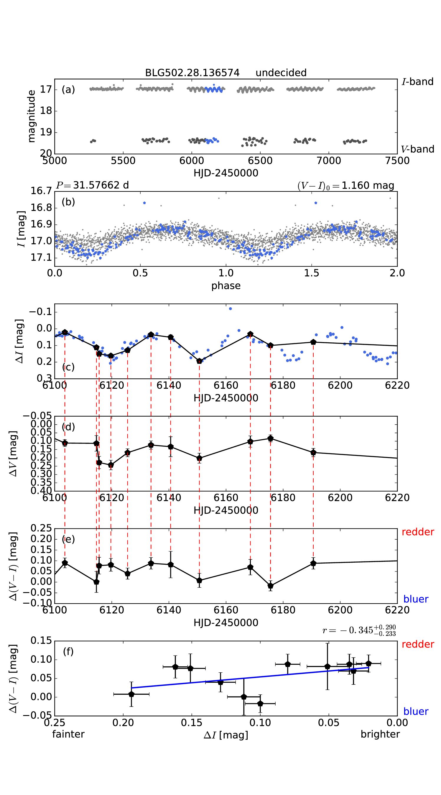
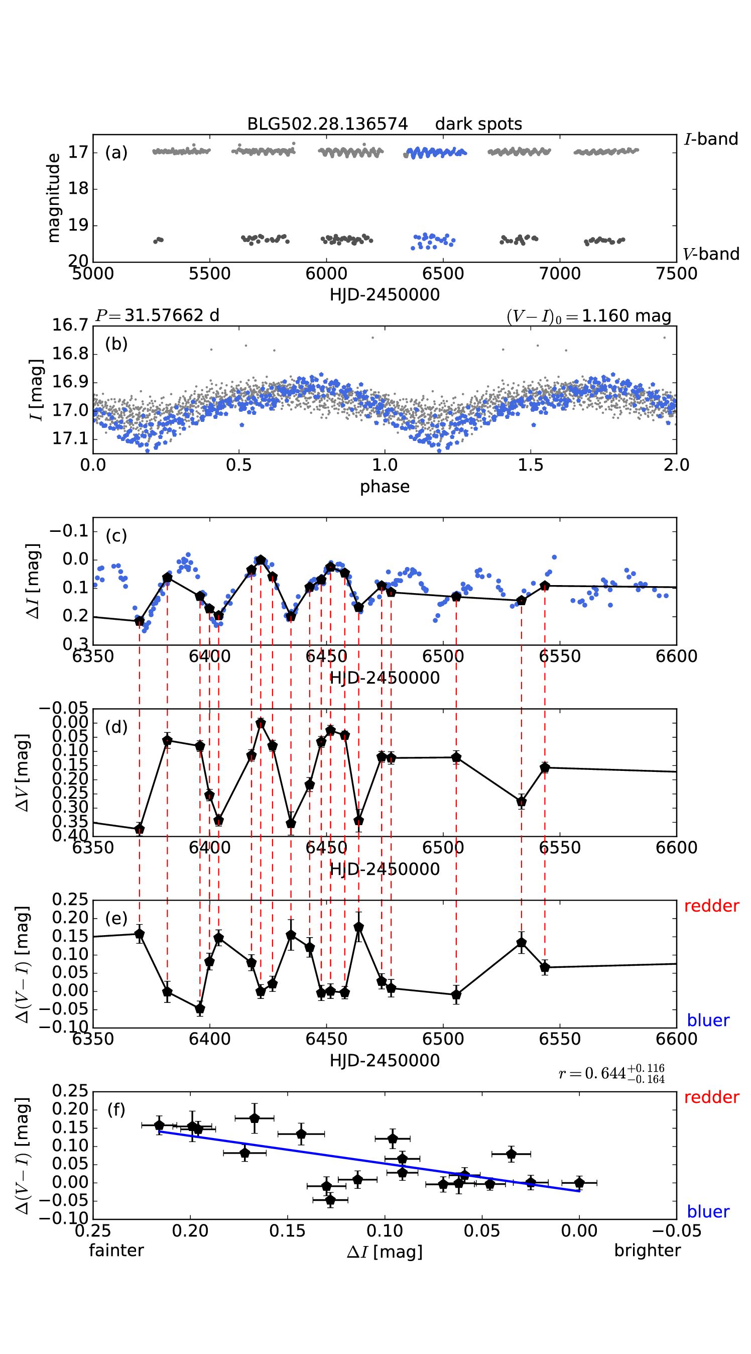
Figure 17.— Example of the evolution of starspots. Both panels show the same star (BLG502.28.136574) in two different intervals of time. This is the star for which the correlation coefficient is around zero ($r=0.163_{-0.117}^{+0.112}$) over the entire time-span of observations. In the time range HJD$-2450000\in[6100,6220]$ there is no, or only the slight negative correlation, which would suggests the apparent existence of chemical spots on the stellar surface, or very small impact of dark spots on the brightness and color of the star. On the other hand, in the time range HJD$-2450000\in[6350,6600]$ the correlation is significant and indicates the existence of dark spots. (a) All observations in both I- and V-bands. Blue points denote the observations analyzed in the further plots. (b) Phase folded light curves with the rotation period given above the plot together with the dereddened color index $(V-I)_{0}$. (c) The I-band variations for the time-span marked in the top plot. Black points show measurements for which we have simultaneous I- and V-band observations. (d) The V-band variations. (e) Color variations. (f) Correlations between color variations and brightness variations. The correlation coefficient calculated in the considered time range is printed above the plot. For better visibility of these correlations we fitted a straight line to the data. All black points are plotted with the appropriate measurement uncertainties in both coordinates.

Thanks to the long-term, well-sampled, two-band OGLE light curves, we are able to study the relation between brightness variability and the color index $(V-I)$ variability. For all stars from our collection, we choose brightness measurements in both filters from the same night, with the time difference between the frames in both colors not exceeding 0.1 day. In the next step, we calculate the $(V-I)$ indices for each pair of brightness measurements. Then we remove all outlying $(V-I)$ measurements, deviating more than $\pm 3\sigma$ from the median. As a result of these calculations we are left with several, up to several dozen brightness measurements in both filters and the color indices $(V-I)$. Subsequently, we take the maximum measured brightness in the I-band ($I_{max}$) for each object, the corresponding V-band ($V_{max}$) magnitude and the color index ($(V-I)_{max}$). Then we calculate $\Delta I$, $\Delta V$ and $\Delta(V-I)$ as follows:

$$\Delta I=I-I_{max},$$ (6)

$$\Delta V=V-V_{max},$$ (7)

$$\Delta(V-I)=(V-I)-(V-I)_{max}.$$ (8)

For the uncertainty of brightness changes we use appropriate values as reported in the light curves. We calculate the uncertainty for changes in color as:

$$\varepsilon(V-I)=\sqrt{dV^{2}+dI^{2},}$$ (9)

where $dV$ and $dI$ are brightness uncertainties as reported in the light curves.

We expect that the brightness of a star with cool, dark spots should decrease when highly spotted area is on the visible side of a star and the color should change to a redder one. Indeed, we detect such a correlation for some of the stars in our sample. An example of such a behavior is shown in Figure 16 (left panel). However, we also detect a number of objects with the opposite dependence between the luminosity and color changes – the stars are more luminous, when the color is redder (Figure 16, right panel).

For all the stars from our sample we calculate the relations between the luminosities and colors. We use bootstrapping method to estimate the correlation coefficient with appropriate uncertainties. For each star we randomly draw with returning brightness in I-band and color $(V-I)$ along the measurement uncertainties. We made 1000 draws, during which we calculate the correlation coefficient. In the next step, we calculate 16th, 50th and 84th percentiles of the correlation coefficient distribution. We assume that we will use the 50th percentile (the median of the correlation coefficient) for further analysis with uncertainties calculated as follows:

$$\sigma_{+}=50\mathrm{th}-16\mathrm{th},$$ (10)

$$\sigma_{-}=84\mathrm{th}-50\mathrm{th},$$ (11)

$$\sigma_{\pm}=\frac{\sigma_{+}+\sigma_{-}}{2}.$$ (12)

In addition, we remove from our sample the stars with $\sigma_{\pm}>0.3$ because of a statistically insignificant correlation due to e.g. a too low number of points. These calculations leave $11\,412$ (out of $12\,660$) stars with statistically significant correlation between brightness and color variations.

From $11\,412$ stars that show statistically significant correlation we find 5199 objects with the positive correlation coefficient ($r-\sigma_{-}\geq 0.2$; left panel in Figure 16) and 465 stars with the negative correlation coefficient ($r+\sigma_{+}\leq-0.2$, right panel in Figure 16). Positive correlation coefficient means that a star is redder (and cooler) when it is less luminous, which is a clear confirmation of the existence of cool, dark spots on the surface. For this reason, we successively name this group as “dark spots”. On the other hand, a negative correlation coefficient means a lot more puzzling behavior – a star is redder when it is more luminous. It is worth mentioning, however, that both types of correlations are related to rotation periods, which is a strong evidence of the existence of spots on the stellar surfaces. Additionally, both spots’ behaviors result from differences in brightness amplitudes measured in the I- and V-band. It is seen from Figure 16 that the positive correlation coefficient means that the amplitude in the V-band is larger than in I-band. It is opposite for stars showing the negative correlation coefficient; here the amplitude in the V-band is smaller than in I-band. One scenario that can explain a lower amplitude in the V-band, and cyclic reddening of the star is connected with chemical spots on the stellar surface. The overabundance of heavy elements inside a spot related to the surface magnetic field can cause a phenomenon called line-blanketing which depresses the short-wavelength part of the electromagnetic spectrum (Milne, 1928). The line-blanketing depends on the wavelength, because the number and the strength of spectral lines of the overabundant elements increases with decreasing wavelength. The energy absorbed at short wavelengths is re-emitted at long wavelengths due to the backwarming effect. This causes a star to become fainter at shorter wavelengths and brighter at longer wavelengths hence redder (e.g. Gray and Corbally 2009). This effect is very well known for Ap stars (e.g. Molnar 1973; Stępień and Czechowski 1993). Recently, Sikora et al. (2019) analyzed all known chemically peculiar stars located closer than 100 pc from the Sun and showed that they all have spectral types earlier than late F. Assuming F8 as the limiting spectral type we obtain the corresponding color index $(V-I)_{0}=0.5$ mag. In addition, the observations of many field Ap stars over several decades indicate that their average brightnesses and amplitudes of their light curves are remarkably stable. So only stars from our sample hotter than the above limit (allowing, of course, for uncertainty of the derived extinction-free indices) and showing the same properties can be considered as candidate Ap (or, alternatively, CP) stars. Definite confirmation of their classification should come from spectroscopic observations.

In another scenario that can explain the observed changes with the negative correlation we can consider a system of two stars with a cool, tidally distorted component and a hotter companion. Many such systems are known as RS CVn-type binaries. Let us assume that the orbit inclination is too low for eclipses to occur but large enough to see light variability due to ellipticity of the cool component. At the maximum light we see both stars from the side. The increased contribution from the red star results in reddening of the system. At the minimum light we see the red star almost end-on and its contribution is diminished. The color index becomes bluer. Additionally, the spots evolution on the cool component surface can also contribute to the total light variations of the system. Note that there is no a priori limit on $(V-I)_{0}$ for stars in this category. On the other hand, the negative correlation was noticed in Young Stellar Objects, and was explained as a significant change in the structure of the inner disk (e.g. Günther et al. 2014; Wolk et al. 2015; Rebull et al. 2015; Wolk et al. 2018).

The remaining 5748 objects show the correlation coefficient around 0 ($r+\sigma_{+}>-0.2$ and $r-\sigma_{-}<0.2$), so we named this group “undecided”. The apparent lack of correlation may result from a variable combination of dark spots and bright areas (like faculae, plages or quiescent prominences) in magnetically active stars or a specific combination of different elements in chemical spots of chemically peculiar stars. Activity variation in the course of activity cycles will also blur the correlation. One example of this situation is presented in Figure 17. Looking at the light curve of the same star in different epochs, it is clearly seen that at a time we do not see any significant spot-induces modulation of brightness and color (see the left panel of Fig. 17), but somewhat later measurable changes of the brightness and color of the star are clearly visible (right panel in Fig. 17). Note that in the left panel of Fig. 17, the amplitudes in both filters are comparable. About 100 days later, when the dark spots appear on the stellar surface (right panel in Fig. 17), the amplitude in V-band becomes larger.

In the remaining part of the paper we use the correlation coefficients calculated from the entire OGLE-IV data when discussing both types of spots (dark and chemical), whereas the correlation coefficients presented in both panels of Figures 16 and 17 are calculated only over the time ranges marked with blue points.

Figure 18.— Color–magnitude diagram (CMD) for stars, for which we found statistically significant dependencies between brightness variations and color variations ($\sigma_{\pm}\leq 0.3$). Isochrones are the same as in Fig. 8. The color bar on the right describes the correlation coefficient.

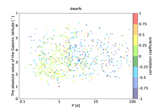
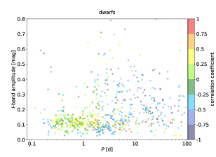
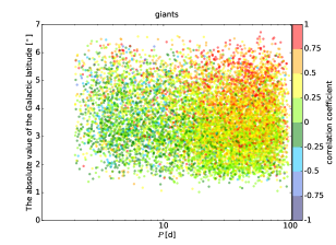
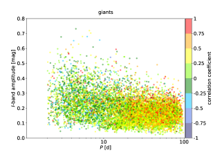
Figure 19.— Relations between the absolute value of the Galactic latitude $|b|$ and the rotation period $P$ (left panels), and between the I-band amplitude and the rotation period $P$ (right panels), separately for dwarfs (top panels) and giants (bottom panels) as functions of the color-coded correlation coefficient. Only stars with the statistically significant correlation coefficients, i.e. when $\sigma_{\pm}\leq 0.3$, are plotted.

7.1. Type of spots on the color–magnitude diagram

Using the dereddened color $(V-I)_{0}$, brightness $I_{0}$ (see Section 5) and the statistically significant correlation coefficient ($\sigma_{\pm}\leq 0.3$), we can place each spotted star in the CMD and search for any possible connection between a given type of spots and the star’s location in CMD. This kind of CMD, with color-coded correlation coefficient is presented in Figure 18.

Detection of two different, linear relations between the color and brightness changes, and the separation of a group of stars with the correlation coefficient close to 0 allowed us to obtain a very interesting picture in the CMD diagram. Looking at Figure 18 we distinguish four interesting points related to the spotted stars:

1. We find $161$ and $255$ dwarfs with the positive and negative correlation coefficient, respectively. It means that the majority of stars classified as dwarfs have negative correlation coefficients, which points toward chemical spots on their surfaces. By contrast, only $210$ giants (out of several thousands) show the measurable negative correlation.

2. A systematic change of the correlation coefficient is visible along the Main Sequence (MS). Stars located in the upper part of the MS, bluer than $(V-I)_{0}\approx 0.7$ mag, have mostly negative coefficients. The limit of 0.7 mag corresponds to the cool boundary of chemically peculiar stars (e.g. Sikora et al. 2019), where strong overabundances of heavy elements are detected (e.g. Paunzen et al. 2015, 2016), blurred by the uncertainties in the color index. The number of dwarfs with the negative correlation rapidly decreases in the lower part of the MS where more stars with the positive correlation, indicative of cool spots, occur.

3. The majority of giants show positive correlation coefficients – they have dark spots on their surfaces. The giants with the negative correlation occur almost exclusively close to the bottom of the giant branch.

4. The correlation coefficient varies smoothly along the giant branch, from the negative value at its bottom, through zero in the middle part up to the largest positive values at the top. The boundaries between the successive values of the correlation coefficient seem to have slopes similar to the isoradius lines.

From the above results we conclude that the chemical spots or variations characteristic of RS CVn-type stars with favorably inclined orbits (producing negative correlation between light and color variations) occur in hotter MS stars and slightly evolved giants. Mildly evolved giants and some cool dwarfs show the simultaneous presence of dark spots and bright areas indicative of high level of activity. Other cool MS stars and evolved giants show predominance of dark spots.

7.2. Correlations overview

Now we discuss in detail two out of five relations presented in Section 6), taking into account the values of the correlation coefficients between light and color variations. These are period-absolute value of the Galactic latitude $|b|$ (left panels of Fig. 19), and period-I-band amplitude (right panels of Fig. 19), separately for dwarfs and giants. The individual data points are colored according to the value of the correlation coefficient as coded by the bar on the right-hand side of each Figure.

It is seen that most of the fast rotating stars with $P\leq 2$ d (all assumed to be dwarfs) have positive values of the correlation coefficient – out of 146 stars from this range 97 show positive correlation. These are cool, rapidly rotating dwarfs covered with dark spots. On the other hand, negative correlation coefficients prevail in slowly rotating dwarfs – out of 270 stars from this range 206 show negative correlation. A large fraction of them belong to Ap stars. As it is well known, these objects rotate with typical periods from a fraction of a day to a few weeks, although much longer periods, even up to centuries, are also observed (Preston, 1974; Renson and Catalano, 2001; Bychkov et al., 2016; Mathys et al., 2019). Some slowly rotating stars with negative correlation between light and color variations may belong to the RS CVn-type variables as discussed earlier.

A reversed tendency is seen among giants where the negative correlation occurs mostly for stars with periods shorter than 10 days whereas the largest positive values of the correlation coefficient occur in stars with periods longer than 20 days. This is in line with our previous interpretation that giants with shorter periods belong to RS CVn-type variables which, depending on the orbit inclination, may show positive, as well as negative values of the correlation coefficient. Giants rotating with the longest periods may belong to wide binaries or to single, active stars.

The systematic trends of the light curve amplitude and $|b|$ with the period, discussed in Section 6 are confirmed here.

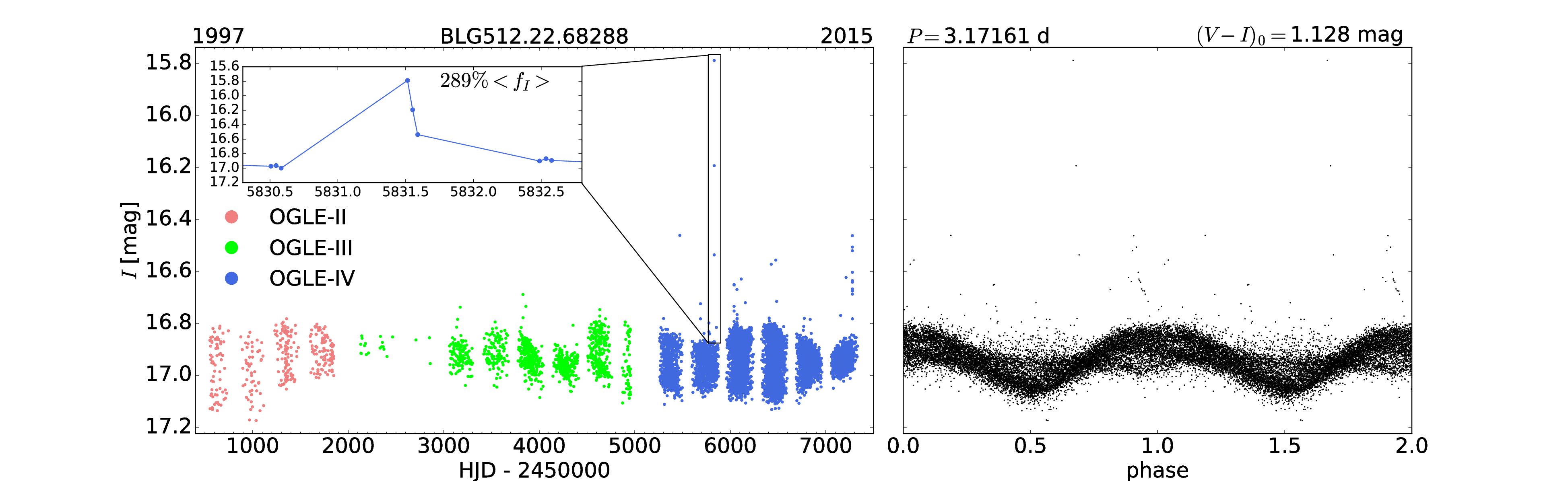
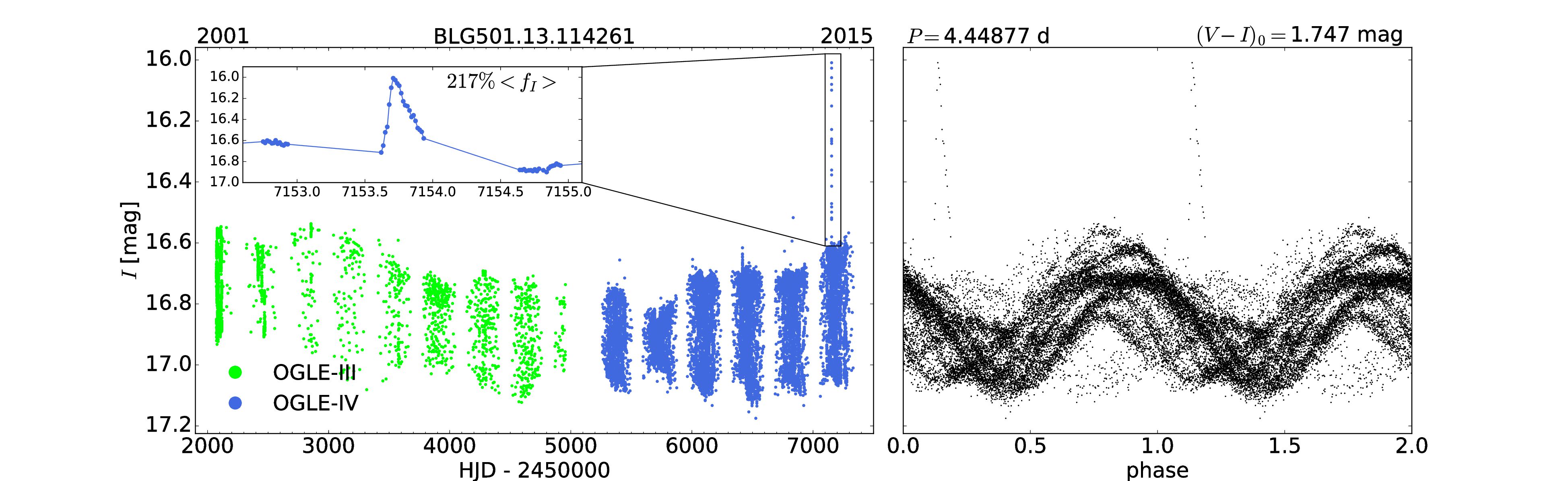
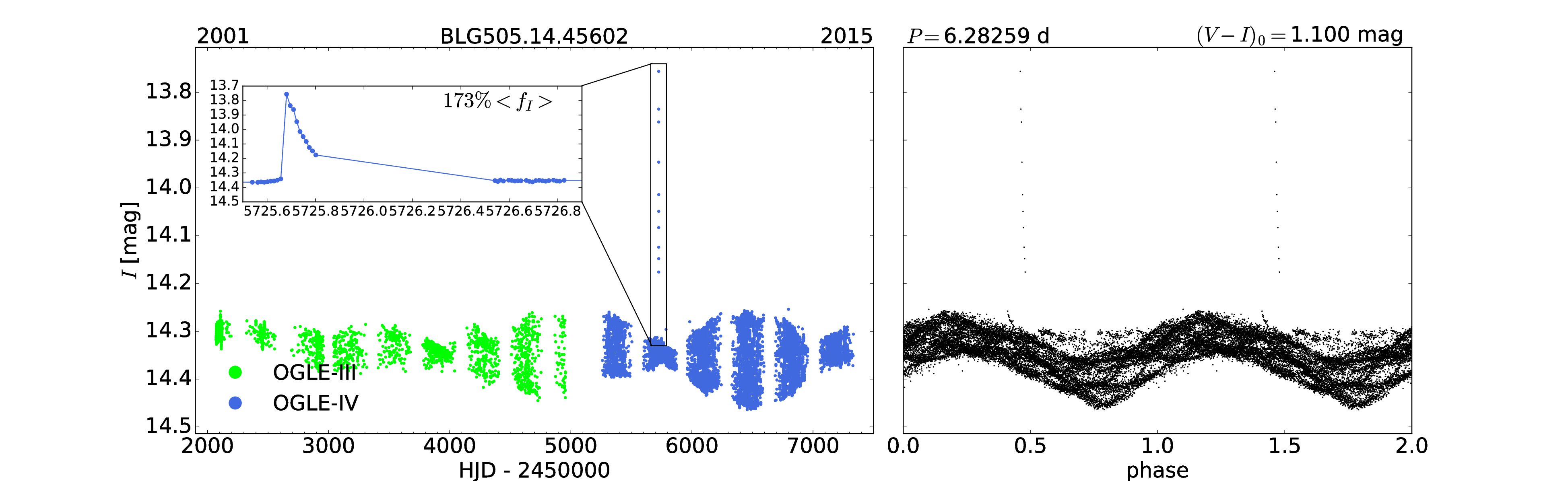
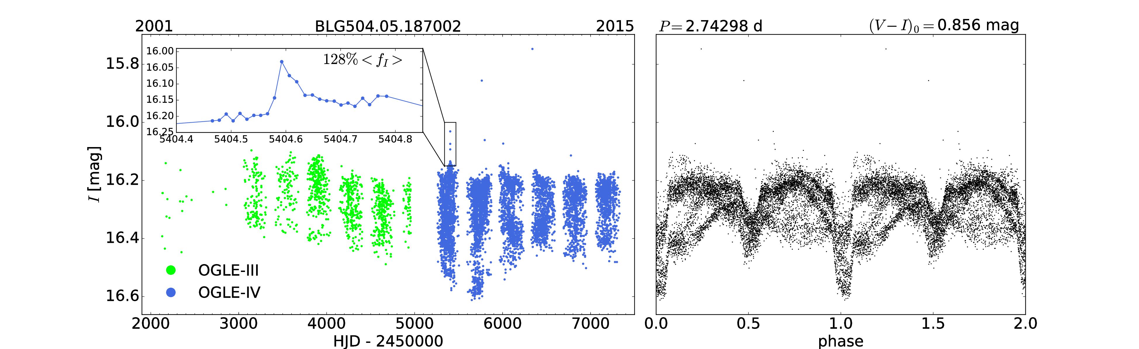
Figure 20.— Four examples of flaring stars found in our collection of spotted stars. Left panels show time-domain light curves, right panels show phased light curves with rotation periods $P$, given above the phased plot. Next to the periods we also provide dereddened color index $(V-I)_{0}$. The dates over non-phased plot refer to the moment when the observations started, and the year from which the last observations come. The consecutive phases of the OGLE project are marked with different colors. Inset graphs present the zoomed flares together with the amount of star’s brightening during the flare relative to its mean brightness.

8. Flaring stars

Besides spots, flares are another determinant of the stellar magnetic activity. Many years of research of active stars have shown that flares occur in stars of all spectral types – from O to late M (e.g. Marchenko et al. 1998; Balona 2012; Maehara et al. 2012; Hawley et al. 2014; Yang et al. 2017). Classical flaring events in cool stars are a phenomenon of a sudden release of energy accumulated by the magnetic field in active regions due to the magnetic reconnection, while flares in hot stars probably are caused by shocks and radiatively driven winds (e.g. Balona 2012). It is also possible that flares observed in hot stars are not produced by these stars, but by a cooler companion. The sudden release of energy is manifested by a rapid brightening of the star, followed by a slow decline. Typical time-scales of the flares range from minutes to several hours or even days (e.g. Henry & Newsom 1996). Flaring events can be observed almost along the entire spectrum of the electromagnetic radiation – from X-rays to radio waves. It is well known that flares on the solar surface have energies between $10^{25}$ erg and $10^{32}$ erg (Shimizu, 1995; Emslie et al., 2012). However, Maehara et al. (2012) detected 1000 times more energetic flares (called superflares) on the solar-type stars. Drake (2006) found no evidence of flares among the thousands of light curves of chromospherically active stars from the MACHO data. The absence of flaring events in the MACHO data was the motivation to look for flaring events in our collection of spotted stars.

8.1. Search for flares

Flares can be detected as outlying points in the light curves. We search for flaring events in two steps. In the first step we looked for outliers deviating by $-4\sigma$ from the mean brightness among all of the light curves from our sample. This automatic scan returned 3582 stars as candidates for flaring objects. Further classification was based solely on the visual inspection of the pre-selected light curves. When at least three consecutive points deviate from the periodic light curve, we consider such an event as a flare. In each case we also check for a characteristic asymmetry between the rising and decaying branch. This search returned 79 stars as almost certain objects with flare phenomenon. It is important to note that the flare detection efficiency strongly depends on the cadence of the observations – some of the OGLE fields have been observed more often than the others (see Udalski et al. 2015). Obviously, some flares have been observed completely, some in part, and some must have been missed. The impact of the cadence on the flares detection efficiency has been discussed e.g. by Yang et al. (2018). The outliers occurring in stars located in the fields that were observed less frequently could look like measurement errors (e.g. cosmic rays) and were rejected during our classification. In Figure 20, we present four examples of light curves with flares from our collection.

With the optical data only, it is impossible to measure the entire energy released during an outburst, because we lack necessary values of the stellar parameters. Because of that, we decided to calculate the relative brightening during a flare for each star classified as a flaring object. We convert the mean brightness over the time span of the observations and the flare maximum brightness into fluxes. The relative brightening can be defined as:

$$\frac{\Delta f_{I}}{\left<f_{I}\right>}\cdot 100\%=\frac{f_{I,\mathrm{max}}-\left<f_{I}\right>}{\left<f_{I}\right>}\cdot 100\%,$$ (13)

where $f_{I,\mathrm{max}}$ is the flare maximum flux and $\left<f_{I}\right>$ is a mean flux over the time span of the observations. We calculated the relative brightening for the highest data point during the flaring event. It is worth mentioning, however, that the maximum recorded brightness during the outburst might not correspond to the true flare brightness maximum – as we discussed it earlier, it is strongly dependent on the cadence of the observations. The relative brightenings of the flares are provided in insets of Figure 20. The upper row of Figure 20 shows a light curve with the largest brightening found in our collection (BLG512.22.68288) equal to $289\%\left<f_{I}\right>$. The value of $289\%\left<f_{I}\right>$ means that during this flare the star brightened by $189\%$ above the average brightness level.

8.2. Flaring stars in the color–magnitude diagram

In Figure 21, we present location of flaring stars in the CMD. Using our dereddening procedure (described in Section 5), we note that 11 flaring stars are dwarfs, and 68 are giants. Recent research shows, that flares on the giant stars are not unusual (e.g. Van Doorsselaere et al. 2017). It is worth mentioning, however, that our detection efficiency for dwarfs is much smaller than for giants because we are not able to detect dwarfs located in the Galactic bulge due to their low brightness and strong interstellar extinction.

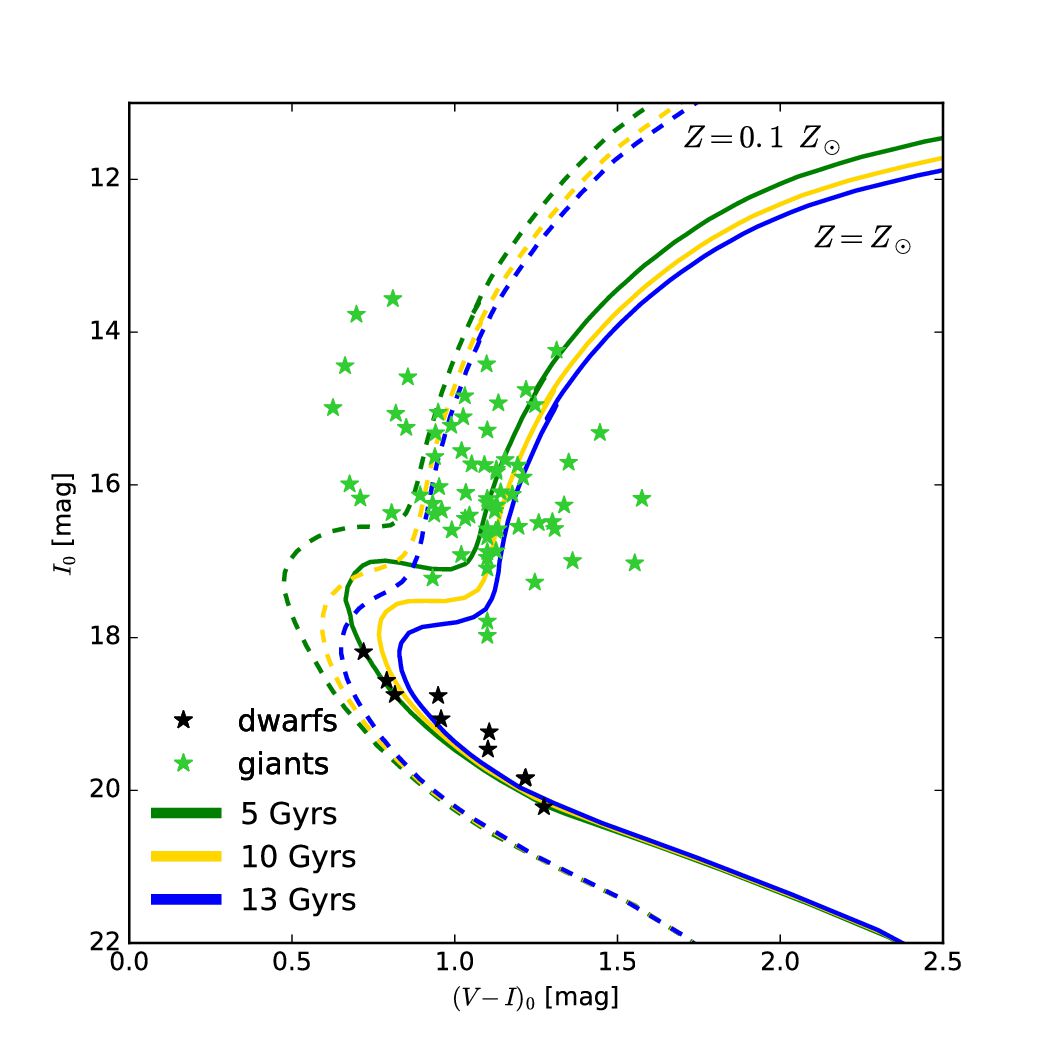
Figure 21.— Color–magnitude diagram (CMD) for flaring stars found in our collection of spotted variables. Isochrones are the same as in Fig. 8.

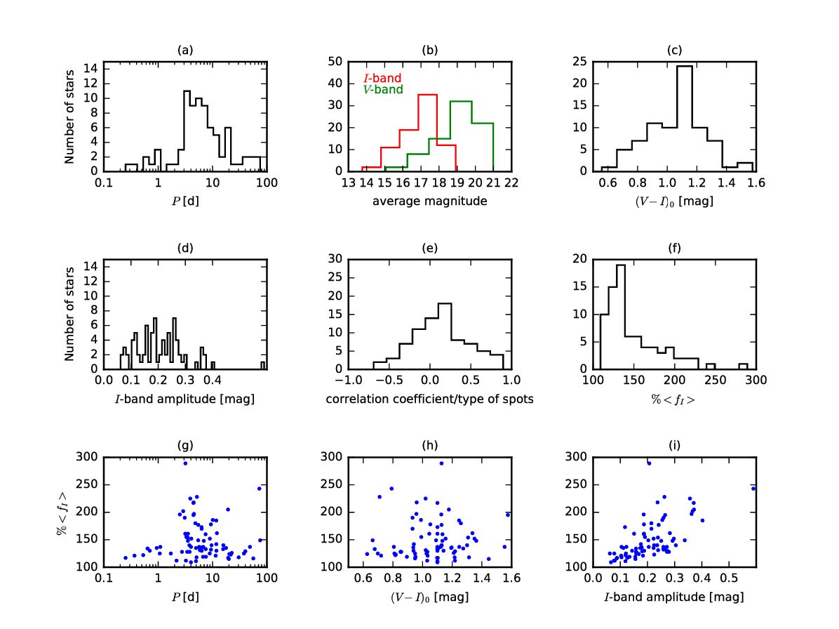
Figure 22.— Basic statistical properties of flaring stars. (a) The histogram of the rotation periods $P$. (b) The histogram of the average magnitudes in both filters. (c) The histogram of the dereddened color indices $(V-I)_{0}$. (d) The histogram of the I-band amplitudes. (e) The histogram of the correlation coefficients, which is related to the type of spots occurring on stellar surfaces. (f) The histogram of the observed values of the relative flare brightenings. (g) Dependence between relative flare brightening and rotation period $P$. (h) Dependence between relative flare brightening and dereddened color index $(V-I)_{0}$. (i) Dependence between relative flare brightening and the mean I-band amplitude.

8.3. Basic statistical properties of flaring stars

In this section we investigate the basic statistical properties of the 79 stars in which we detected flares. Figure 22 shows five histograms with different parameters of the flaring stars: the rotation periods (Figure 22a), average magnitudes (Figure 22b), color indices $(V-I)_{0}$ (Figure 22c), I-band amplitudes (Figure 22d) and the correlation coefficients between periodic light and color variations (Figure 22e). In Figure 22f, we present the distribution of flares with different relative brightenings. The three bottom diagrams (Figures 22g, h and i) are the plots of relative brightening versus rotation period, color index $(V-I)_{0}$ and I-band amplitude.

The rotation periods of our flare stars are within the range $0.251\leq P\leq 75.132$ d (Figure 22a) with the maximum number of flaring objects occurring for $2\leq P<4$ d. A range of the rotation periods is wide, what may suggests that the occurrence of flares does not depend on how fast a star rotates. However, Maehara et al. (2017) showed that the flare occurrence rate depends on rotation period. The small number of stars with rotation periods shorter than about 3 days results very likely from the low number of all investigated stars with these periods.

The most common values of the I-band brightness of flaring stars occur in the range $16.9$-$17.9$ mag. By comparing Figure 22b with Figure 2 we can conclude that stars with flares are on average less luminous than other spotted stars for which the most common values of the I-band brightness are in the range $16.7$-$16.9$ mag. A similar difference is observed in the V-band.

It is well known that most of the flaring stars are red (e.g. Davenport 2016; Yang et al. 2017; Van Doorsselaere et al. 2017). Indeed, 52 of our flaring stars ($66\%$) have colors $(V-I)_{0}\geq 1.0$ mag with a peak at $(V-I)_{0}\approx 1.1$ mag corresponding to the spectral type of K4-K5 (Figure 22c). The highest brightening with the value of $289\%$ (BLG512.22.68288; upper panel in Figure 20) was also found in a red star, with a color index $(V-I)_{0}=1.128$ mag. This is consistent with the common belief that most active are the red stars. Flares also appear on blue stars, but mechanisms responsible for such events are still under discussion (e.g. Balona 2012; Pedersen et al. 2017). The bluest object from our sample of flaring stars has $(V-I)_{0}=0.626$ mag.

Amplitudes of periodic brightness variations are related to spot sizes, their lifetimes, asymmetry in the surface distribution, migration and evolution. The amplitudes of the flaring stars do not seem to differ significantly from the bulk of the observed amplitudes although only two of them exceeds 0.4 mag (Figures 22d, i). This is probably the effect of a small number of spotted stars with larger amplitudes. It is worth mentioning, however, that the correlation between the relative flare brightening and the mean I-band amplitude measured over the time interval of the OGLE observations is clearly visible (Figure 22i). It seems that stars with larger brightness amplitudes (and thus larger spots coverage) produce more energetic flares, what is indirect confirmation of the work done by Yang et al. (2017), who found a positive correlation between the starspot size and the flare activity in M dwarfs. However, they also found that some of the M dwarfs with strong flares do not exhibit any light variations caused by the starspots.

Using the same method as in Section 7, we check which types of spots are observed in flaring stars (Figure 22e). All these stars show statistically significant correlation coefficients between the light and color variations ($\sigma_{\pm}\leq 0.3$)but the extreme values close to $-1$ or $1$ are rarely present. The majority of the flare stars is grouped around the null correlation coefficient. It seems that frequently flaring stars show the less stable brightness-color correlation, and thus the faster evolving spots and more strongly variable magnetic fields.

Most of the flare brightenings does not exceed $150\%$ (52 stars out of 79; Figure 22f). This means that strong outbursts in which the star’s brightness increases twice or more are infrequent. It is an indirect confirmation of Maehara’s (2012) research, who found only 148 stars with superflares among $83\;000$ stars from the Kepler data.

9. Conclusions

In this paper, we presented the detection and statistical analysis of $12\;660$ spotted stars lying toward, and in the Galactic bulge. We introduced a new dereddening procedure, as the bulge is one of the most challenging regions of the sky to explore due to the large, irregular interstellar extinction. As an result of our analysis we classified $848$ spotted stars as dwarfs and $11\;812$ stars as giants. In the first part of this work, we conducted a similar analysis to that done by Drake (2006), what allowed us to confirm accurately some of the correlations reported by them, and to analyze these correlations in greater details. Moreover, we found previously unknown interesting features of the spotted variables. The second part of our paper contains the analysis based on the brightness-color correlation we have disclosed. We found 79 flaring objects among all spotted variables and we examined their statistical properties.

Our analysis shows that the correlation between the Galactic latitude and rotation period of giants reported by Drake (2006) is probably caused by the selection effect. We think this is an artifact of the period magnitude relation existing for giants which means that it is harder to detect faster rotating hence fainter giants due to the increasing extinction close to the Galactic plane. We also did not confirm the period-color relation suggested by Drake (2006). Four times larger sample of stars does not show any systematic trend of color with period. On the other hand, our data show a clear correlation between luminosity and rotation period which is not visible in the data analyzed by Drake (2006). We confirm that fainter stars from our sample show larger brightness variations, and thus larger and/or more nonuniform spots coverage. However, the existence of this correlation is most likely a selection effect – for fainter stars we were able to detect only large amplitudes. It is noteworthy, however, that bright stars ($I_{0}\lesssim 16$ mag) do not show amplitudes larger than 0.4 mag. This is an unexpected finding and it seems to be real. We notice that the spotted stars can be divided into two groups: fast-rotating ($P\leq 2$ d) dwarfs with small amplitudes (I-band amplitude $<0.2$ mag), and slow-rotating dwarfs and giants with amplitudes of up to 0.8 mag. The existence of these two distinct, well-resolved groups suggests that the mechanisms responsible for spot formation, thus the magnetic activity, may differ between these two classes. On the other hand, large amplitudes are recorded on stars with large spots coverage, but with clear longitudinal asymmetry in spotted areas. Uniformly spotted stars or with dominant polar spots will produce very small brightness variations despite the heavy spot coverage on their surfaces. In such cases another measure of the magnetic activity should be used e.g. core emission in the calcium lines CaII H and K (Baliunas et al., 1995) or X-ray flux (Pallavicini et al., 1981). Hereafter, we indicate both groups as interesting for a more detailed study. The correlation between the I-band amplitude and rotation period for giants is clearly visible – the slower a giant rotates, the smaller amplitude it shows. By contrast, slow rotating dwarfs seem to show larger amplitudes than the rapidly rotating ones.

Using accurate, long-term, two-band OGLE photometry we revealed the existence of the correlation between brightness variations and color variations of the spotted variables. We find that based on the value of the correlation coefficient stars from our collection can be divided into three groups according to the strength of this correlation. This dependence is an indicator of which type of spots prevails on the stellar surface. First group contains stars which show positive correlation coefficient ($r-\sigma_{-}\geq 0.2$) what suggests that variability is due to the existence of dark, cool spots on the stellar surface. Second group consists of stars with the negative correlation coefficient ($r+\sigma_{+}\leq-0.2$). Negative values of the coefficient mean that the stars are redder when more luminous because their brightness variations in the V-band are smaller than in I-band. This kind of variations can be produced by nonuniform distribution of elements over the stellar surface i.e. chemical spots associated with the stable magnetic field. The increased abundance of heavy elements in a chemical spot rotating with the star results in a variable line-blanketing effect. Field chemically peculiar stars are observed only among early spectral type stars. It would be valuable to observe spectroscopically our Ap star candidates to confirm their status. The negative correlation observed in cool stars may result from the rotation of a tidally distorted cool component in a binary of the RS CVn-type variable with a favorable orbit inclination. Observations show that the correlation coefficients are remarkably stable throughout the OGLE-IV phase. This suggests that spots are slowly evolving and their lifetimes can be very long. Going further, we can expect that the magnetic fields on these stars should be quite stable on the time scale of at least a decade. The last group contains stars for which the correlation coefficient is around 0 ($r+\sigma_{+}>-0.2$ and $r-\sigma_{-}<0.2$). It seems that stars from the last group have rapidly evolving spots together with variable bright regions hence their surface magnetic field rapidly vary in time, which makes the correlation between brightness and color blurred. A very interesting result is obtained when all the spotted stars are plotted in the CMD with the correlation coefficient color coded. All three groups are clearly separated with the coefficient varying along the MS from the negative values for the hottest stars, through null values up to the positive values for the coolest dwarfs. In the case of giants the coefficient varies along the giant branch: the negative correlation prevails among least massive giants and its value increases with the giant mass. The lines of constant coefficient lie approximately along the lines of constant stellar radius. This would suggest that the type of this correlation depends on the stellar radius, and thus on the strength and configuration of the surface magnetic fields. Among our spotted stars we found 79 objects with flare footprints. Our results show that the correlation coefficient of the flaring stars is concentrated around null value. This indicates that these stars have unstable, fast-evolving magnetic fields producing frequent outbursts. Moreover, correlation between the flare brightening and the I-band amplitude is clearly visible. We also notice that slow rotators show the highest brightenings during flares, however stars with very strong flares, at least doubling the stellar brightness are very rare.

10. Acknowledgments

We are grateful to the anonymous Referee for the careful reading of our manuscript and for his/her supportive and constructive comments which greatly improved this publication. We also thank the anonymous Statistics Consultant for important comments related to the Fourier time-series analysis. Thanks to these remarks the Section about period searching has been significantly expanded. We would like to thank Profs. M. Kubiak, G. Pietrzyński and Dr. M. Pawlak for their contribution to the collection of the OGLE photometric data over the past years. We are grateful to late Z. Kołaczkowski for discussion and ideas that improved this paper.

This work has been supported by the National Science Centre, Poland, grant MAESTRO no. 2016/22/A/ST9/00009 to I. Soszyński. P. Iwanek is partially supported by the “Kartezjusz” programme no. POWR.03.02.00-00-I001/16-00 founded by the National Centre for Research and Development, Poland. The OGLE project has received funding from the National Science Center, Poland, grant MAESTRO no. 2014/14/A/ST9/00121 to A. Udalski.

References

- Alard & Lupton (1998) Alard, C., Lupton, R. H., 1998, ApJ, 503, 325
- Alcock et al. (1995) Alcock, C., Allsman, R. A., Axelrod, T. S., Bennett, D. P., Cook, K. H., Freeman, K. C., Griest, K., Marshall, S. L., Peterson, B. A., Pratt, M. R., Quinn, P. J., Reimann, J., Rodgers, A. W., Stubbs, C. W., Sutherland, W., Welch, D. L., 1995, AJ, 109, 1653
- Baliunas et al. (1995) Baliunas, S. L., Donahue, R. A., Soon, W. H., Horne, J. H., Frazer, J., Woodard-Eklund, L., Bradford, M., Rao, L. M., Wilson, O. C., Zhang, Q., Bennett, W., Briggs, J., Carroll, S. M., Duncan, D. K., Figueroa, D., Lanning, H. H., Misch, T., Mueller, J., Noyes, R. W., Poppe, D., Porter, A. C., Robinson, C. R., Russell, J., Shelton, J. C., Soyumer, T., Vaughan, A. H., Whitney, J. H., 1995, ApJ, 438, 269
- Balona (2012) Balona, L. A., 2012, MNRAS, 423, 3420
- Balona et al. (2015) Balona, L. A., Baran, A. S., Daszyńska-Daszkiewicz, J., De Cat, P., 2015, MNRAS, 451, 1445
- Balona (2017) Balona, L. A., 2017, MNRAS, 467, 1830
- Basri et al. (2011) Basri, G., Walkowicz, L. M., Batalha, N., Gilliland, R. L., Jenkins, J., Borucki, W. J., Koch, D., Caldwell, D., Dupree, A. K., Latham, D. W., Marcy, G. W., Meibom, S., Brown, T., 2011, AJ, 141, 20
- Basri et al. (2013) Basri, G., Walkowicz, L. M., Reiners, A., 2013, ApJ, 769, 37
- Bressan et al. (2012) Bressan, A., Marigo, P., Girardi, L., Salasnich, B., Dal Cero, C., Rubele, S., Nanni, A., 2012, MNRAS, 427, 127
- Bychkov et al. (2016) Bychkov, V. D., Bychkova, L. V., Madej, J., 2016, MNRAS, 455, 2567
- Ceillier et al. (2017) Ceillier, T., Tayar, J., Mathur, S., Salabert, D., García, R. A., Stello, D., Pinsonneault, M. H., van Saders, J., Beck, P. G., Bloemen, S., 2017, A&A, 605, 111
- Davenport (2016) Davenport, R. A. J., 2016, ApJ, 829, 23
- Drake (2006) Drake, A. J., 2006, AJ, 131, 1044
- Drake et al. (1989) Drake, S. A., Simon, T., Linsky, J. L., 1989, ApJS, 71, 905
- Durney and Latour (1978) Durney, B. R., Latour, J., 1978, GApFD, 9, 241
- Emslie et al. (2012) Emslie, A., Dennis, B., Shih, A., Chamberlin, P., Mewaldt, R., Moore, C., Share, G., Vourlidas, A., Welsch, B., 2012, ApJ, 759, 71
- Gaia Collaboration (2018) Gaia Collaboration; Brown, A. G. A., et al., 2018, A&A, 616, 1
- Gaia Collaboration (2016) Gaia Collaboration; Prusti, T., et al., 2016, A&A, 595, 1
- Gray and Corbally (2009) Gray, R. O., Corbally, J. C., 2009, Princeton University Press, ISBN: Â 978-0-691-12511-4
- Guerrero et al. (2013) Guerrero, G., Smolarkiewicz, P. K., Kosovichev, A. G., Mansour, N. N., 2013, ApJ, 779, 176
- Guerrero et al. (2016a) Guerrero, G., Smolarkiewicz, P. K., de Gouveia Dal Pino, E. M., Kosovichev, A. G., Mansour, N. N., 2016 ApJ, 819, 104
- Guerrero et al. (2016b) Guerrero, G., Smolarkiewicz, P. K., de Gouveia Dal Pino, E. M., Kosovichev, A. G., Mansour, N. N., 2016, ApJ, 828, 3
- Guerrero et al. (2018) Guerrero, G., Zaire, B., Smolarkiewicz, P. K., de Gouveia Dal Pino, E. M., Kosovichev, A. G., Mansour, N. N., 2018, eprint arXiv:1810.07978
- Günther et al. (2014) Günther, H. M., Cody, A. M., Covey, K. R., Hillenbrand, L. A., Plavchan, P., Poppenhaeger, K., Rebull, L. M., Stauffer, J. R., Wolk, S. J., Allen, L., Bayo, A., Gutermuth, R. A., Hora, J. L., Meng, H. Y. A., Morales-Calderón, M., Parks, J. R., Song, I., 2014, AJ, 148, 122
- Guthnick and Prager (1914) Guthnick, P., Prager, R., 1914, Veröff. Berlin-Babelsberg, 1, 44
- Hawley et al. (2014) Hawley, S. L., Davenport, J. R. A., Kowalski, A. F., Wisniewski, J. P., Hebb, L., Deitrick, R., Hilton, E. J., 2014, ApJ, 797, 121
- Henry & Newsom (1996) Henry, G. W., Newsom, M. S., 1996, PASP, 108, 242
- Hoffmeister (1915) Hoffmeister, C., 1915, \an, 200, 177
- Hubrig et al. (2019) Hubrig, S., Küker, M., Järvinen, S. P., Kholtygin, A. F., Schöller, M., Ryspaeva, E. B., Sokoloff, D. D., 2019, MNRAS, 484, 4495
- Hurley et al. (2000) Hurley, J. R., Pols, O. R., Tout, C. A., 2000, MNRAS, 315, 543
- Irwin et al. (2009) Irwin, J., Aigrain, S., Bouvier, J., Hebb, L., Hodgkin, S., Irwin, M., Moraux, E., 2009, MNRAS, 392, 1456
- Kiraga (2012) Kiraga, M., 2012, Acta Astron., 62, 67
- Kiraga and Stępień (2013) Kiraga, M., Stępień, K., 2013, Acta Astron., 63, 53
- Kochukhov et al. (2019) Kochukhov, O., Shultz, M., Neiner, C., 2019, A&A, 621, 47
- Kochukhov and Shulyak (2019) Kochukhov, O., Shulyak, D., 2019, eprint arXiv:1902.04157
- Kraft (1967) Kraft, R. P., 1967, ApJ, 150, 551
- Kron (1947) Kron, G. E., 1947, PASP, 59, 261
- Kron (1950) Kron, G. E., 1950, ASPL, 6, 52
- Kurtz (1985) Kurtz, D. W., 1985, MNRAS, 213, 773
- Lanzafame et al. (2018a) Lanzafame, A. C., Distefano, E., Barnes, S. A., Spada, F., 2018, eprint arXiv:1805.11332
- Lanzafame et al. (2018b) Lanzafame, A. C., Distefano, E., Messina, S., Pagano, I., Lanza, A. F., Eyer, L., Guy, L. P., Rimoldini, L., Lecoeur-Taibi, I., Holl, B., Audard, M., de Fombelle, G. J., Nienartowicz, K., Marchal, O., Mowlavi, N., 2018, A&A, 616, 16
- Lomb (1976) Lomb, N. R., 1976, Ap&SS, 39, 447
- Maehara et al. (2012) Maehara, H., Shibayama, T., Notsu, S., Notsu, Y., Nagao, T., Kusaba, S., Honda, S., Nogami, D., Shibata, K., 2012, Nature, 485, 478
- Maehara et al. (2017) Maehara, H., Notsu, Y., Notsu, S., Namekata, K., Honda, S., Ishii, T. T., Nogami, D., Shibata, K., 2017, PASJ, 69, 41
- Marchenko et al. (1998) Marchenko, S., Moffat, A., van der Hucht, K., Seggewiss, W., Schrijver, H., Stenholm, B., Lundstrom, I., Setia Gunawan, D., Sutantyo, W., van den Heuvel, E., de Cuyper, J.-P., Gomez, A., 1998, A&A, 331, 1022
- Mathur et al. (2014) Mathur, S., García, R. A., Ballot, J., Ceillier, T., Salabert, D., Metcalfe, T. S., Régulo, C., Jiménez, A., Bloemen, S., 2014, A&A, 562, 124
- Mathys et al. (2019) Mathys, G., Romanyuk, I. I., Hubrig, S., Kudryavtsev, D. O., Landstreet, J. D., Schöller, M., Semenko, E. A., Yakunin, I. A., 2019, eprint arXiv:1902.05869
- Maury and Pickering (1897) Maury, A. C., Pickering, E. C., 1897, AnHar, 28, 1
- McQuillan et al. (2014) McQuillan, A., Mazeh, T., Aigrain, S., 2014, ApJS, 211, 24
- Mekkaden (1985) Mekkaden, M. V., 1985, Ap&SS, 117, 381
- Messina and Guinan (2002) Messina, S., Guinan, E. F., 2002, A&A, 393, 225
- Milne (1928) Milne, E. A., 1928, \theobservatory, 51, 88
- Molnar (1973) Molnar, M. R., 1973, ApJ, 179, 527
- Montet et al. (2017) Montet, B. T., Tovar, G., Foreman-Mackey, D., 2017 ApJ, 851, 116
- Nataf et al. (2013) Nataf, D. M., Gould, A., Fouqué, P., Gonzalez, O. A., Johnson, J. A., Skowron, J., Udalski, A., Szymański, M. K., Kubiak, M., Pietrzyński, G., Soszyński, I., Ulaczyk, K., Wyrzykowski, Ł., Poleski, R., 2013, ApJ, 769, 88
- Oláh & Strassmeier (2002) Oláh, K., Strassmeier, K. G., 2002, \an, 323, 361
- Oláh et al. (2009) Oláh, K., Kolláth, Z., Granzer, T., Strassmeier, K. G., Lanza, A. F., Järvinen, S., Korhonen, H., Baliunas, S. L., Soon, W., Messina, S., Cutispoto, G., 2009, A&A, 501, 703
- Oláh et al. (2016) Oláh, K., Kövári, Zs., Petrovay, K., Soon, W., Baliunas, S., Kolláth, Z., Vida, K., 2016, A&A, 590, 133
- Pallavicini et al. (1981) Pallavicini, R., Golub, L., Rosner, R., Vaiana, G.S., Ayres, T., Linsky, J. L., 1981, ApJ, 248, 279
- Parker (1955) Parker, E. N., 1955, ApJ, 122, 293
- Pedersen et al. (2017) Pedersen, M. G., Antoci, V., Korhonen, H., White, T. R., Jessen-Hansen, J., Lehtinen, J., Nikbakhsh, S., Viuho, J., 2017, MNRAS, 466, 3060
- Paunzen et al. (2015) Paunzen, E., Fröhlich, H.-E., Netopil, M., Weiss, W. W., Lüftinger, T., 2015, A&A, 574, 57
- Paunzen et al. (2016) Paunzen, E., Netopil, M., Bernhard, K., Hümmerich, S., 2016, BlgAJ, 24, 97
- Pojmański (1997) Pojmański, G., 1997, Acta Astron., 47, 467
- Pojmański (2002) Pojmański, G., 2002, Acta Astron., 52, 397
- Preston (1974) Preston, G. W., 1974, ARA&A, 12, 257
- Rebull et al. (2015) Rebull, L. M., Stauffer, J. R., Cody, A. M., Günther, H. M., Hillenbrand, L. A., Poppenhaeger, K., Wolk, S. J., Hora, J., Hernandez, J., Bayo, A., Covey, K., Forbrich, J., Gutermuth, R., Morales-Calderón, M., Plavchan, P., Song, I., Bouy, H., Terebey, S., Cuillandre, J. C., Allen, L. E., 2015, AJ, 150, 175
- Reinhold et al. (2017) Reinhold, T., Cameron, R. H., Gizon, L., 2017, A&A, 603, 52
- Renson and Catalano (2001) Renson, P., Catalano, F. A., 2001, A&A, 378, 113
- Roettenbacher et al. (2016) Roettenbacher, R. M., Monnier, J. D., Korhonen, H., Aarnio, A. N., Baron, F., Che, X., Harmon, R. O., Kövàri, Zs., Kraus, S., Schaefer, G. H., Torres, G., Zhao, M., Ten Brummelaar, T. A., Sturmann, J., Sturmann, L., 2016, Nature, 533, 217
- Ross (1926) Ross, F. E., 1926, AJ, 36, 124
- Salabert et al. (2016) Salabert, D., García, R. A., Beck, P. G., Egeland, R., Pallé, P. L., Mathur, S., Metcalfe, T. S., do Nascimento, J.-D., Jr., Ceillier, T., Andersen, M. F., Triviñ o Hage, A., 2016, A&A, 596, 31
- Scargle (1982) Scargle, J. D., 1982, ApJ, 263, 835
- Schlegel et al. (1998) Schlegel, D. J., Finkbeiner, D. P., Davis, M., 1998, ApJ, 500, 525
- Schwabe (1844) Schwabe, H., 1844, \an, 21, 233
- Schwabe (1845) Schwabe, H., 1845, \an, 22, 365
- Serenelli et al. (2016) Serenelli, A., Scott, P., Villante, F.L., Vincent, A.C., Asplund, M., Basu, S., Grevesse, N., Penã-Garay, C., 2016, MNRAS, 463, 2
- Sharma et al. (2011) Sharma, S., Bland-Hawthorn, J., Johnston, K. V., Binney, J., 2011, ApJ, 730, 3
- Shimizu (1995) Shimizu, T., 1995, PASJ, 47, 251
- Sikora et al. (2019) Sikora, J., Wade, G. A., Power, J., Neiner, C., 2019, MNRAS, 483, 2300
- Simon & Fekel (1987) Simon, T., Fekel, F.C. Jr., 1987, ApJ, 316, 434
- Skumanich (1972) Skumanich A., 1972, ApJ, 171, 565
- Soszyński et al. (2013) Soszyński, I., Udalski, A., Szymański, M. K., Kubiak, M., Pietrzyński, G., Wyrzykowski, Ł., Ulaczyk, K., Poleski, R., Kozłowski, S., Pietrukowicz, P., Skowron, J., 2013, Acta Astron., 63, 21
- Soszyński et al. (2016) Soszyński, I., Pawlak, M., Pietrukowicz, P., Udalski, A., Szymański, M. K., Wyrzykowski, Ł., Ulaczyk, K., Poleski, R., Kozłowski, S., Skowron, D. M., Skowron, J., Mróz, P., Hamanowicz, A., 2016, Acta Astron., 66, 405
- Stępień (1968) Stępień, K., 1968, ApJ, 154, 945
- Stępień and Czechowski (1993) Stępień, K., Czechowski, W., 1993, A&A, 268, 187
- Strassmeier et al. (2019) Strassmeier, K. G., Carroll, T. A., Ilyin, I. V., 2019, eprint arXiv:1902.11201
- Szymański et al. (2011) Szymański, M. K., Udalski, A., Soszyński, I., Kubiak, M., Pietrzyński, G., Poleski, R., Wyrzykowski, Ł., Ulaczyk, K., 2011, Acta Astron., 61, 83
- Udalski et al. (2002) Udalski, A., Szymański, M., Kubiak, M., Pietrzyński, G., Soszyński, I., Woźniak, P., Zebruń, K., Szewczyk, O., Wyrzykowski, Ł., 2002, Acta Astron., 52, 217
- Udalski et al. (2015) Udalski, A., Szymański, M. K., Szymański, G., 2015, Acta Astron., 65, 1
- Udalski et al. (2018) Udalski, A., Soszyński, I., Pietrukowicz, P., Szymański, M. K., Skowron, D. M., Skowron, J., Mróz, P., Poleski, R., Kozłowski, S., Ulaczyk, K., Rybicki, K., Iwanek, P., Wrona, M., 2018 Acta Astron., 68, 315
- VanderPlas (2018) VanderPlas, J. T., 2019, ApJS, 236, 16
- Van Doorsselaere et al. (2017) Van Doorsselaere, T., Shariati, H., Debosscher, J., 2017, ApJS, 232, 26
- von Steiger & Zurbuchen (2016) von Steiger, R., Zurbuchen, T. H., 2016, ApJ, 816, 13
- Wade et al. (2016) Wade, G. A., Neiner, C., Alecian, E., Grunhut, J. H., Petit, V., Batz, B. de, Bohlender, D. A., Cohen, D. H., Henrichs, H. F., Kochukhov, O., Landstreet, J. D., Manset, N., Martins, F., Mathis, S., Oksala, M. E., Owocki, S. P., Rivinius, Th., Shultz, M. E., Sundqvist, J. O., Townsend, R. H. D., ud-Doula, A., Bouret, J.-C., Braithwaite, J., Briquet, M., Carciofi, A. C., David-Uraz, A., Folsom, C. P., Fullerton, A. W., Leroy, B., Marcolino, W. L. F., Moffat, A. F. J., Nazé, Y., Louis, N. St., Auriére, M., Bagnulo, S., Bailey, J. D., Barbá, R. H., Blazére, A., Böhm, T., Catala, C., Donati, J.-F., Ferrario, L., Harrington, D., Howarth, I. D., Ignace, R., Kaper, L., Lüftinger, T., Prinja, R., Vink, J. S., Weiss, W. W., Yakunin, I., 2016, MNRAS, 456, 2
- Wolk et al. (2015) Wolk, S. J., Günther, H. M., Poppenhaeger, K., Cody, A. M., Rebull, L. M., Forbrich, J., Gutermuth, R. A., Hillenbrand, L. A., Plavchan, P., Stauffer, J. R., Covey, K. R., Song, I., 2015, AJ, 150, 145
- Wolk et al. (2018) Wolk, S. J., Günther, H. M., Poppenhaeger, K., Winston, E., Rebull, L. M., Stauffer, J. R., Gutermuth, R. A., Cody, A. M., Hillenbrand, L. A., Plavchan, P., Covey, K. R., Song, I., 2018, AJ, 155, 99
- Woźniak (2000) Woźniak, P. R., 2000, Acta Astron., 50, 421
- Yang et al. (2017) Yang, H., Liu, J., Gao, Q., Fang, X., Guo, J., Zhang, Y., Hou, Y., Wang, Y., Cao, Z., 2017, ApJ, 849, 36
- Yang et al. (2018) Yang, H., Liu, J., Qiao, E., Zhang, H., Gao, Q., Cui, K., Han, H., 2018, ApJ, 859, 87