A Matrix-in-matrix Neural Network for Image Super Resolution

Abstract

In recent years, deep learning methods have achieved impressive results with higher peak signal-to-noise ratio in single image super-resolution (SISR) tasks by utilizing deeper layers. However, their application is quite limited since they require high computing power. In addition, most of the existing methods rarely take full advantage of the intermediate features which are helpful for restoration. To address these issues, we propose a moderate-size SISR network named matrixed channel attention network (MCAN) by constructing a matrix ensemble of multi-connected channel attention blocks (MCAB). Several models of different sizes are released to meet various practical requirements. Conclusions can be drawn from our extensive benchmark experiments that the proposed models achieve better performance with much fewer multiply-adds and parameters. Our models will be made publicly available at this URL .

HR Bicubic SRCNN [7] FSRCNN[8] DRCN[21] VDSR[20] DRRN[32] LapSRN [23] CARN-M [1] CARN [1] MCAN-FAST (ours) MCAN (ours)

Figure 1: Visual results with bicubic degradation ($\times$4) on “img_092” from Urban100.

1 Introduction

Single image super-resolution (SISR) attempts to reconstruct a high-resolution (HR) image from its low-resolution (LR) equivalent, which is essentially an ill-posed inverse problem since there are infinitely many HR images that can be downsampled to the same LR image.

Most of the works discussing SISR based on deep learning have been devoted to achieving higher peak signal noise ratios (PSNR) with deeper and deeper layers, making it difficult to fit in mobile devices [20, 21, 32, 41]. Out of many proposals, an architecture CARN has been released that is applicable in the mobile scenario, but it is at the cost of reduction on PSNR [1]. An information distillation network (IDN) proposed in [18] also achieves good performance at a moderate size. An effort that tackles SISR with neural architecture search has also been proposed [5, 6], their network FALSR surpasses CARN at the same level of FLOPS.

Still, there is a noticeable gap between subjective perception and PSNR, for which a new measure called perceptual index (PI) has been formulated [3]. Noteworthy works engaging perceptual performance are SRGAN [24] and ESRGAN [36], which behave poorly on PSNR but both render more high-frequency details. However, these GAN-based methods inevitably bring about bad cases that are intolerable in practice. Our work still focuses on improving PSNR, which is a well-established distortion measure. Furthermore, our proposed model can also serve as the generator of GAN-based methods.

To seek a better trade-off between performance and applicability, we design an architecture called Matrixed Channel Attention Network. We name its basic building block multi-connected channel attention block (MCAB), which is an adaptation of residual channel attention block (RCAB) from RCAN [41]. MCAB differs from RCAB by allowing hierarchical connections after each activation, in such way, multiple levels of information can be passed both in depth and in breadth.

In summary, our main contributions are as follows:

• We propose a matrixed channel attention network named MCAN for SISR. It scores higher PSNR and achieves the state-of-the-art results within a lightweight range.

• We introduce a multi-connected channel attention block to construct matrixed channel attention cell (MCAC), which makes full use of the hierarchical features. Then we use MCAC to build a matrix-in-matrix (MIM) structure that serves as a nonlinear mapping module.

• We devise an edge feature fusion (EFF) block, which can be used in combination with the proposed MIM structure. The EFF can better profit the hierarchical features of MIM from the LR space.

• We build three additional efficient SR models of different sizes, i.e., MCAN-M, MCAN-S, MCAN-T, which are respectively short for mobile, small, and tiny. Experiments prove that all three models outperform the state-of-the-art models of the same or bigger sizes.

• We finally present MCAN-FAST to overcome the inefficiency of the sigmoid function on some mobile devices. Experiments show that MCAN-FAST has only a small loss of precision compared to MCAN.

2 Related Works

In recent years, deep learning has been applied to many areas of computer vision [11, 14, 26, 30, 39]. A pioneering work [7] has brought super-resolution into deep learning era, in which they proposed a simple three-layer convolutional neural network called SRCNN, where each layer sequentially deals with feature extraction, non-linear mapping, and reconstruction. The input of SRCNN, however, needs an extra bicubic interpolation which reduces high-frequency information and adds extra computation. Their later work FSRCNN [8] requires no interpolation and inserts a deconvolution layer for reconstruction, which learns an end-to-end mapping. Besides, shrinking and expanding layers are introduced to speed up computation, altogether rendering FSRCNN real-time on a generic CPU.

Meantime, VDSR presented by [21] features a global residual learning to ease training for their very deep network. DRCN handles deep network recursively to share parameters [21]. DRRN builds two residual blocks in a recursive manner [32]. They all bear the aforementioned problem caused by interpolation. Furthermore, these very deep architectures undoubtedly require heavy computation.

The application of DenseNet in SR domain goes to SRDenseNet [35], in which they argue that dense skip connections mitigate the vanishing gradient problem and can boost feature propagation. It achieves better performance as well as faster speed. However, results from [5] showed that dense connection might not be the most efficient and their less dense network FALSR is also competitive.

Later, a cascading residual network CARN is devised for a lightweight scenario [1]. The basic block of their architecture is called cascading residual block, whose outputs of intermediary layers are dispatched to each of the consequent convolutional layers. These cascading blocks, when stacked, are again organized in the same fashion.

There is another remarkable work RCAN [41], which has a great impact on our work. They have observed that low-frequency information is hard to capture by convolutional layers which only exploit a local region. By adding multiple long and short skip connections for residual dense blocks, low-frequency features can bypass the network and thus the main architecture focuses on high-frequency information. They also invented a channel attention mechanism via global average pooling to deal with interdependencies among channels.

3 Matrixed Channel Attention Network

3.1 Network Structure

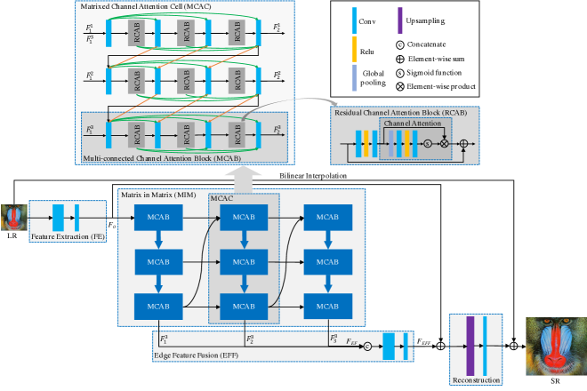
Figure 2: The architecture of matrixed convolutional neural network (MCAN), in which MIM is set to $D=3,K=3,M=3$. (The blue thick arrows indicate multiple connections between two blocks).

The MCAN consists of four components: feature extraction (FE), matrix in matrix (MIM) mapping, edge feature fusion (EFF) and reconstruction, as illustrated in Figure 2.

Specifically, we utilize two successive $3\times 3$ convolutions to extract features from the input image in the FE stage. Let $I_{LR}$ represent the input image and $I_{HR}$ be the output, this procedure can then be formulated as

$$\begin{split}F_{0}&=H_{FE}(I_{LR})\end{split}$$ (1)

where $H_{FE}(\cdot)$ is the feature extraction function and $F_{0}$ denotes the output features.

The nonlinear mapping is constructed by what we call a matrix-in-matrix module (MIM). Similarly,

$$\begin{split}F_{EF}&=H_{MIM}(F_{0})\end{split}$$ (2)

where $H_{MIM}(\cdot)$ is the mapping function, to be discussed in detail in Section  3.2. $F_{EF}$ stands for the edge features, so named for they are coming from the edge of our matrix block. Further feature fusion can be put formally as,

$$\begin{split}F_{EFF}&=H_{EFF}(F_{EF}),\end{split}$$ (3)

We will elaborate on EFF in Section 3.4.

Lastly, we upscale the combination of fused feature $F_{EFF}$ and $F_{0}$to generate the high-resolution target via reconstruction,

$$\begin{split}I_{SR}&=H_{UP}(F_{EFF}+F_{0})+U(I_{LR}),\end{split}$$ (4)

where $H_{UP}(\cdot)$ denotes the upsampling function and $U(\cdot)$ the bilinear interpolation.

3.2 Matrix in Matrix

The MIM block contains $D=3$ matrixed channel attention cells (MCAC). A single MCAC is again a sequence of $M=3$ MCABs. The $d$-th MCAC relays intermediate features to the next MCAC. In fact, each MCAC contains $K=3$ heads, which are fed into different parts of the next MCAC. We recursively define $F_{d}$ as the outputs of a MCAC,

$$\begin{split}F_{d}&=H_{MCAC}^{d}(F_{d-1})\\ &=H_{MCAC}^{d}((F_{d-1}^{1},F_{d-1}^{2},\dots,F_{d-1}^{K}))\\ &=(F_{d}^{1},F_{d}^{2},\dots,F_{d}^{K}).\\ \end{split}$$ (5)

Thence the output of $H_{MIM}(\cdot)$ can be composed by the combination of $K$-th outputs of all MCACs,

$$\begin{split}F_{EF}&=(F_{1}^{K},F_{2}^{K},\dots,F_{D}^{K}).\\ \end{split}$$ (6)

Therefore, we can regard MIM as a $D\times K$ matrix. If we look at its structural detail, a MCAC can again be seen as a matrix of $K\times M$, for this reason we call it matrix-in-matrix. The overall structure of MIM is shown in Figure 2.

3.3 Matrixed Channel Attention Cell

In super-resolution, skip connections are popular since it reuses intermediate features while relieving the training for deep networks [21, 27, 35]. Nevertheless, these skip connections between modules are point-to-point, where only the output features of a module can be reused, losing many intermediate features. This can be alleviated by adding skip connections within the module, but as more intermediate features are concatenated, channels become very thick before fusion [42], which narrows transmission of information and gradients.

If we densely connect all intermediate features and modules like the SRDenseNet [35], it inevitably brings in redundant connections for less important features, while the important ones become indistinguishable and increases the training difficulty.

To address these problems, we propose a matrixed channel attention cell, which is composed of several multi-connected channel attention blocks.

3.3.1 Multi-connected Channel Attention Block

Previous works seldom discriminate feature channels and treat them equally. Till recently a channel attention mechanism using global pooling is proposed in RCAN to concentrate on more useful channels [41]. We adopt the same channel attention block RCAB as in RCAN, also depicted in Figure 2, and the difference of the two only lies in the style of connections.

Channel Attention Mechanism. We let $X=[x_{1},\cdots,x_{c},\cdots,x_{C}]$ denote an input that contains $C$ feature maps, and the shape of each feature map be $H\times W$. Then the statistic $z_{c}$ of $c$-th feature map $x_{c}$ is defined as

$$\begin{split}z_{c}&=H_{GP}(x_{c})=\dfrac{\sum_{i=1}^{H}\sum_{j=1}^{W}x_{c}(i,j)}{H\times W},\\ \end{split}$$ (7)

where $x_{c}(i,j)$ denotes the value at index $(i,j)$ of feature map $x_{c}$, and $H_{GP}(\cdot)$ represents the global average pooling function. The channel attention of the feature map $x_{c}$ can thus be denoted as

$$\begin{split}s_{c}&=f(W_{U}\delta(W_{D}z_{c})),\end{split}$$ (8)

where $f(\cdot)$ and $\delta(\cdot)$ represent the sigmoid function and the ReLU [29] function respectively, $W_{D}$ is the weight set of a $1\times 1$ convolution for channel downscaling. This convolution reduces the number of channels by a factor $r$. Later after being activated by a ReLU function, it enters a $1\times 1$ convolution for channel upscaling with the weights $W_{U}$, which expands the channel again by the factor $r$. The computed statistic $s_{c}$ is used to rescale the input features ${x_{c}}$,

$$\begin{split}\hat{x}_{c}&=s_{c}\cdot x_{c},\end{split}$$ (9)

Description of RCAB. The RCAB is organized using the aforementioned channel attention mechanism. Formally it can be seen as a function $H_{RCAB}(\cdot)$ on the input features $I$,

$$\begin{split}F_{RCAB}&=H_{RCAB}(I)\\ &=s_{X_{I}}\cdot X_{I}+I\\ &=\hat{X}_{I}+I,\end{split}$$ (10)

where $s_{X_{I}}$ is the output of channel attention on $X_{I}$, which are the features generated from the two stacked convolution layers,

$$\begin{split}X_{I}&=W_{2}\delta(W_{1}I).\end{split}$$ (11)

The cascading mechanism from CARN [1] makes use of intermediate features in a dense way. In order to relax the redundancy of dense skip connections, our residual channel attention blocks are built in a multi-connected fashion, so called as MCAB, as shown in Figure 2. Each MCAB contains $M$ residual channel attention blocks (RCAB) and $M+1$ pointwise convolution operations for feature fusion ($H_{F}$), which are interleaved one after another.

3.3.2 MCAC Structure

The structure of MCAC can be considered as a matrix of $K=3$ MCABs times $M=3$ RCABs. In the $d$-th MCAC, we let the input and output of $k$-th MCAB be ${IM}_{d}^{k}$ and ${OM}_{d}^{k}$, and the $k$-th output of the last MCAC be $F_{d-1}^{k}$, we formulate ${IM}_{d}^{k}$ as follows,

$$\left\{\begin{array}[]{lr}\text{$[F_{0}]$}&d=k=0\\ \text{$[{OM}_{d}^{k-1}]$}&d=0,k\in(0,K]\\ \text{$[F_{d-1}^{k}]$}&d\in(0,D],k=0\\ \text{$[{OM}_{d}^{k-1},F_{d-1}^{k}]$}&d\in(0,D],k\in(0,K]\\ \end{array}\right.$$ (16)

In the case of $d\in(0,D],k\in(0,K],m\in(0,M]$, the $m$-th feature fusion convolution $H_{F}$ takes multiple inputs and fuses them into $F_{d}^{k,m}$. Let the input of $m$-th RCAB be ${IR}_{d}^{k,m}$ and the output ${OR}_{d}^{k,m}$, we can write the input of $m$-th feature fusion convolution ${IF}_{d}^{k,m}$ as,

$$\left\{\begin{array}[]{lr}\text{$[$}F_{d-1}^{k},F_{d}^{k-1,m+1},F_{d}^{k-1,M+1}\text{$]$}&m=0\\ \text{$[$}{OR}_{d}^{k,m-1},F_{d}^{k-1,m+1},F_{d}^{k,1},\\ \hskip 14.22636pt\dots,F_{d}^{k,m-1}\text{$]$}&m\in(0,M]\\ \text{$[$}{OR}_{d}^{k,m-1},F_{d}^{k,1},\dots,F_{d}^{k,M}\text{$]$}&m=M+1\\ \end{array}\right.$$ (21)

Now we give the complete definition of the output of $d$-th MCAC,

$$\begin{split}F_{d}&=(F_{d}^{1},F_{d}^{2},\dots,F_{d}^{K})\\ &=H_{MCAC,d}(F_{d-1})\\ &=H_{MCAC,d}((F_{d-1}^{1},F_{d-1}^{2},\dots,F_{d-1}^{K}))\\ &=(F_{d}^{1,M+1},F_{d}^{2,M+1},\dots,F_{d}^{K,M+1}).\end{split}$$ (22)

As mentioned above, the nonlinear mapping module of our proposed model can be seen as a matrix of $D\times K$. Thus its overall number of sigmoid functions can be calculated as,

$$\begin{split}num_{f(\cdot)}&=D\times K\times M\times N_{ca},\end{split}$$ (23)

where $f(\cdot)$ means the sigmoid function and $N_{ca}$ indicates the number of filters in the channel attention mechanism.

Method	Scale	Train data	Mult-Adds	Params	Set5	Set14	B100	Urban100
					PSNR/SSIM	PSNR/SSIM	PSNR/SSIM	PSNR/SSIM
SRCNN [7]	$\times$2	G100+Yang91	52.7G	57K	36.66/0.9542	32.42/0.9063	31.36/0.8879	29.50/0.8946
FSRCNN [8]	$\times$2	G100+Yang91	6.0G	12K	37.00/0.9558	32.63/0.9088	31.53/0.8920	29.88/0.9020
VDSR [20]	$\times$2	G100+Yang91	612.6G	665K	37.53/0.9587	33.03/0.9124	31.90/0.8960	30.76/0.9140
DRCN [21]	$\times$2	Yang91	17,974.3G	1,774K	37.63/0.9588	33.04/0.9118	31.85/0.8942	30.75/0.9133
LapSRN [23]	$\times$2	G200+Yang91	29.9G	813K	37.52/0.9590	33.08/0.9130	31.80/0.8950	30.41/0.9100
DRRN [32]	$\times$2	G200+Yang91	6,796.9G	297K	37.74/0.9591	33.23/0.9136	32.05/0.8973	31.23/0.9188
BTSRN [9]	$\times$2	DIV2K	207.7G	410K	37.75/-	33.20/-	32.05/-	31.63/-
MemNet [33]	$\times$2	G200+Yang91	2,662.4G	677K	37.78/0.9597	33.28/0.9142	32.08/0.8978	31.31/0.9195
SelNet [4]	$\times$2	ImageNet subset	225.7G	974K	37.89/0.9598	33.61/0.9160	32.08/0.8984	-
CARN [1]	$\times$2	DIV2K	222.8G	1,592K	37.76/0.9590	33.52/0.9166	32.09/0.8978	31.92/0.9256
CARN-M [1]	$\times$2	DIV2K	91.2G	412K	37.53/0.9583	33.26/0.9141	31.92/0.8960	31.23/0.9194
MoreMNAS-A [6]	$\times$2	DIV2K	238.6G	1,039K	37.63/0.9584	33.23/0.9138	31.95/0.8961	31.24/0.9187
FALSR-A [5]	$\times$2	DIV2K	234.7G	1,021K	37.82/0.9595	33.55/0.9168	32.12/0.8987	31.93/0.9256
MCAN (ours)	$\times$2	DIV2K	191.3G	1,233K	37.91/0.9597	33.69/0.9183	32.18/0.8994	32.46/0.9303
MCAN+ (ours)	$\times$2	DIV2K	191.3G	1,233K	38.10/0.9601	33.83/0.9197	32.27/0.9001	32.68/0.9319
MCAN-FAST (ours)	$\times$2	DIV2K	191.3G	1,233K	37.84/0.9594	33.67/0.9188	32.16/0.8993	32.36/0.9300
MCAN-FAST+ (ours)	$\times$2	DIV2K	191.3G	1,233K	38.05/0.9600	33.78/0.9196	32.26/0.8999	32.62/0.9317
MCAN-M (ours)	$\times$2	DIV2K	105.50G	594K	37.78/0.9592	33.53/0.9174	32.10/0.8984	32.14/0.9271
MCAN-M+ (ours)	$\times$2	DIV2K	105.50G	594K	37.98/0.9597	33.68/0.9186	32.200.8992	32.35/0.9290
MCAN-S (ours)	$\times$2	DIV2K	46.09G	243K	37.62/0.9586	33.35/0.9156	32.02/0.8976	31.83/0.9244
MCAN-S+ (ours)	$\times$2	DIV2K	46.09G	243K	37.82/0.9592	33.49/0.9168	32.12/0.8983	32.03/0.9262
MCAN-T (ours)	$\times$2	DIV2K	6.27G	35K	37.24/0.9571	32.97/0.9112	31.74/0.8939	30.62/0.9120
MCAN-T+ (ours)	$\times$2	DIV2K	6.27G	35K	37.45/0.9578	33.07/0.9121	31.85/0.8950	30.79/0.9137
SRCNN [7]	$\times$3	G100+Yang91	52.7G	57K	32.75/0.9090	29.28/0.8209	28.41/0.7863	26.24/0.7989
FSRCNN [8]	$\times$3	G100+Yang91	5.0G	12K	33.16/0.9140	29.43/0.8242	28.53/0.7910	26.43/0.8080
VDSR [20]	$\times$3	G100+Yang91	612.6G	665K	33.66/0.9213	29.77/0.8314	28.82/0.7976	27.14/0.8279
DRCN [21]	$\times$3	Yang91	17,974.3G	1,774K	33.82/0.9226	29.76/0.8311	28.80/0.7963	27.15/0.8276
DRRN [32]	$\times$3	G200+Yang91	6,796.9G	297K	34.03/0.9244	29.96/0.8349	28.95/0.8004	27.53/0.8378
BTSRN [9]	$\times$3	DIV2K	207.7G	410K	37.75/-	33.20/-	32.05/-	31.63/-
MemNet [33]	$\times$3	G200+Yang91	2,662.4G	677K	34.09/0.9248	30.00/0.8350	28.96/0.8001	27.56/0.8376
SelNet [4]	$\times$3	ImageNet subset	120.0G	1,159K	34.27/0.9257	30.30/0.8399	28.97/0.8025	-
CARN [1]	$\times$3	DIV2K	118.8G	1,592K	34.29/0.9255	30.29/0.8407	29.06/0.8034	28.06/0.8493
CARN-M [1]	$\times$3	DIV2K	46.1G	412K	33.99/0.9236	30.08/0.8367	28.91/0.8000	27.55/0.8385
MCAN (ours)	$\times$3	DIV2K	95.4G	1,233K	34.45/0.9271	30.43/0.8433	29.14/0.8060	28.47/0.8580
MCAN+ (ours)	$\times$3	DIV2K	95.4G	1,233K	34.62/0.9280	30.50/0.8442	29.21/0.8070	28.65/0.8605
MCAN-FAST (ours)	$\times$3	DIV2K	95.4G	1,233K	34.41/0.9268	30.40/0.8431	29.12/0.8055	28.41/0.8568
MCAN-FAST+ (ours)	$\times$3	DIV2K	95.4G	1,233K	34.54/0.9276	30.48/0.8440	29.20/0.8067	28.60/0.8595
MCAN-M (ours)	$\times$3	DIV2K	50.91G	594K	34.35/0.9261	30.33/0.8417	29.06/0.8041	28.22/0.8525
MCAN-M+ (ours)	$\times$3	DIV2K	50.91G	594K	34.50/0.9271	30.44/0.8432	29.14/0.8053	28.39/0.8552
MCAN-S (ours)	$\times$3	DIV2K	21.91G	243K	34.12/0.9243	30.22/0.8391	28.99/0.8021	27.94/0.8465
MCAN-S+ (ours)	$\times$3	DIV2K	21.91G	243K	34.28/0.9255	30.31/0.8403	29.07/0.8034	28.09/0.8493
MCAN-T (ours)	$\times$3	DIV2K	3.10G	35K	33.54/0.9191	29.76/0.8301	28.73/0.7949	26.97/0.8243
MCAN-T+ (ours)	$\times$3	DIV2K	3.10G	35K	33.68/0.9207	29.8/0.8320	28.80/0.7964	27.10/0.8271
SRCNN [7]	$\times$4	G100+Yang91	52.7G	57K	30.48/0.8628	27.49/0.7503	26.90/0.7101	24.52/0.7221
FSRCNN [8]	$\times$4	G100+Yang91	4.6G	12K	30.71/0.8657	27.59/0.7535	26.98/0.7150	24.62/0.7280
VDSR [20]	$\times$4	G100+Yang91	612.6G	665K	31.35/0.8838	28.01/0.7674	27.29/0.7251	25.18/0.7524
DRCN [21]	$\times$4	Yang91	17,974.3G	1,774K	31.53/0.8854	28.02/0.7670	27.23/0.7233	25.14/0.7510
LapSRN [23]	$\times$4	G200+Yang91	149.4G	813K	31.54/0.8850	28.19/0.7720	27.32/0.7280	25.21/0.7560
DRRN [32]	$\times$4	G200+Yang91	6,796.9G	297K	31.68/0.8888	28.21/0.7720	27.38/0.7284	25.44/0.7638
BTSRN [9]	$\times$4	DIV2K	207.7G	410K	37.75/-	33.20/-	32.05/-	31.63/-
MemNet [33]	$\times$4	G200+Yang91	2,662.4G	677K	31.74/0.8893	28.26/0.7723	27.40/0.7281	25.50/0.7630
SelNet [4]	$\times$4	ImageNet subset	83.1G	1,417K	32.00/0.8931	28.49/0.7783	27.44/0.7325	-
SRDenseNet [35]	$\times$4	ImageNet subset	389.9G	2,015K	32.02/0.8934	28.50/0.7782	27.53/0.7337	26.05/0.7819
CARN [1]	$\times$4	DIV2K	90.9G	1,592K	32.13/0.8937	28.60/0.7806	27.58/0.7349	26.07/0.7837
CARN-M [1]	$\times$4	DIV2K	32.5G	412K	31.92/0.8903	28.42/0.7762	27.44/0.7304	25.62/0.7694
MCAN (ours)	$\times$4	DIV2K	83.1G	1,233K	32.33/0.8959	28.72/0.7835	27.63/0.7378	26.43/0.7953
MCAN+ (ours)	$\times$4	DIV2K	83.1G	1,233K	32.48/0.8974	28.80/0.7848	27.69/0.7389	26.58/0.7981
MCAN-FAST (ours)	$\times$4	DIV2K	83.1G	1,233K	32.30/0.8955	28.69/0.7829	27.60/0.7372	26.37/0.7938
MCAN-FAST+ (ours)	$\times$4	DIV2K	83.1G	1,233K	32.43/0.8970	28.78/0.7843	27.68/0.7385	26.53/0.7970
MCAN-M (ours)	$\times$4	DIV2K	35.53G	594K	32.21/0.8946	28.63/0.7813	27.57/0.7357	26.19/0.7877
MCAN-M+ (ours)	$\times$4	DIV2K	35.53G	594K	32.34/0.8959	28.72/ 0.7827	27.63/0.7370	26.34/0.7909
MCAN-S (ours)	$\times$4	DIV2K	13.98G	243K	31.97/0.8914	28.48/0.7775	27.48/0.7324	25.93/0.7789
MCAN-S+ (ours)	$\times$4	DIV2K	13.98G	243K	32.11/0.8932	28.57/0.7791	27.55/0.7338	26.06/0.7822
MCAN-T (ours)	$\times$4	DIV2K	2.00G	35K	31.33/0.8812	28.04/0.7669	27.22/0.7228	25.12/0.7515
MCAN-T+ (ours)	$\times$4	DIV2K	2.00G	35K	31.50/0.8843	28.14/0.7689	27.29/0.7244	25.23/0.7548

Table 1: Quantitative comparison with the state-of-the-art methods based on $\times$2, $\times$3, $\times$4 SR with bicubic degradation model. Red/blue text: best/second-best.

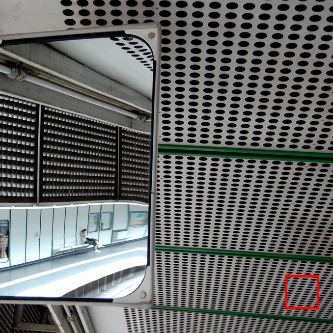
Urban100 ($\times$3): img_004 HR Bicubic FSRCNN[8] VDSR[20] LapSRN [23] CARN [1] PSNR/SSIM 22.87/0.7859 19.72/0.6947 25.01/0.8841 24.82/0.8818 26.15/0.9086 CARN-M [1] MCAN-T (ours) MCAN-S (ours) MCAN-M (ours) MCAN-FAST (ours) MCAN (ours) 24.93/0.8898 24.63/.8748 26.12/0.9051 26.51/0.9125 27.83/0.9259 27.87/0.9281

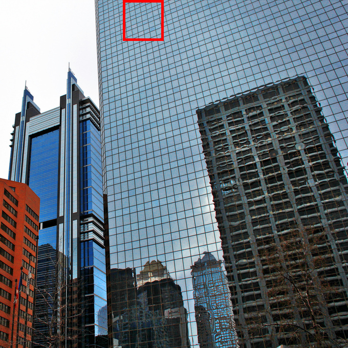
Urban100 ($\times$4): img_099 HR Bicubic FSRCNN[8] VDSR[20] LapSRN [23] CARN [1] PSNR/SSIM 22.41/0.5873 23.61/0.6670 24.02/0.6961 24.47/0.7220 25.81/0.7926 CARN-M [1] MCAN-T (ours) MCAN-S (ours) MCAN-M (ours) MCAN-FAST (ours) MCAN (ours) 25.05/0.7557 24.30/0.7138 25.50/0.7793 25.92/0.7977 25.93/0.8062 26.37/0.8118

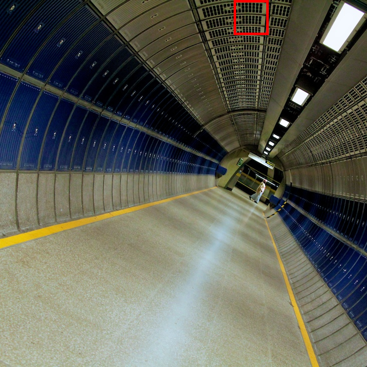
Urban100 ($\times$4): img_078 HR Bicubic FSRCNN[8] VDSR[20] LapSRN [23] CARN [1] PSNR/SSIM 25.70/0.6786 26.46/0.7338 26.80/ 0.7545 26.71/0.7529 27.18/0.7716 CARN-M [1] MCAN-T (ours) MCAN-S (ours) MCAN-M (ours) MCAN-FAST (ours) MCAN (ours) 26.91/0.7597 26.74/0.7492 27.14/0.7678 27.33/0.7745 27.56/0.7809 27.65/0.7824

Figure 3: Visual comparison with bicubic degradation model. Red/blue text: best/second-best.

3.4 Edge Feature Fusion

As we generate multiple features through MIM during different stage, we put forward an edge feature fusion (EFF) module to integrate these features hierarchically.

Particularly, we unite the outputs of the last MCAB in each MCAC, which are nicknamed as the edge of the MIM structure. In further detail, EFF takes a $3\times 3$ convolution for fusion and another $3\times 3$ convolution to reduce channel numbers.

$$\begin{split}F_{EFF}&=W_{F}W_{R}[F_{d}^{1,M+1},\dots,F_{d}^{K,M+1}],\end{split}$$ (24)

where $W_{F}$ and $W_{R}$ are the weights of fusion convolution and the channel reduction layer.

3.5 Comparison with Recent Models

Comparison with SRDenseNet. SRDenseNet uses dense block proposed by DenseNet to construct nonlinear mapping module [35]. This dense connection mechanism may lead to redundancy, in fact not all features should be equally treated. In our work, MIM and EFF can reduce dense connections and highlight the hierarchical information. Additionally, SRDenseNet connects two blocks from point to point, which refrains transmission and utilization of intermediate features. Our proposed multi-connected channel attention block (MCAB) mitigates this problem by injecting multiple connections between blocks.

Comparison with CARN. CARN uses a cascading block [1], which is also pictured in our MIM. Despite of this, MIM features multiple connections between MCACs, and the outputs of different stages are relayed between MCABs. Such an arrangement makes better use of intermediate information. Another important difference is that MCAN combines the hierarchical features before upsampling via edge feature fusion. This mechanism helps significantly for reconstruction.

4 Experimental Results

4.1 Datasets and Evaluation Metrics

We train our model based on DIV2K [34], which contains 800 2K high-resolution images for the training set and another 100 pictures for both validation and test set. Besides, we make comparisons across three scaling tasks ($\times$2, $\times$3, $\times$4) on four datasets: Set5 [2], Set14 [38], B100 [28], and Urban100 [17]. The evaluation metrics we used are PSNR [15] and SSIM [37] on the Y channel in the YCbCr space.

4.2 Implementation Details

As shown in Figure 2, the inputs and outputs of our model are RGB images. We crop the LR patches by $64\times 64$ for various scale tasks and adopt the standard data augmentation.

For training, we use Adam ($\beta_{1}=0.9$, $\beta_{2}=0.999$, and $\epsilon=10^{-8}$) [22] to minimize $L_{1}$ loss within $1.2\times 10^{6}$ steps with a batch-size of $64$. The initial learning rate is set to $2\times 10^{-4}$, halved every $4\times 10^{5}$ steps. Like CARN [1], we also initialize the network parameters by $\theta\sim U(-k,k)$, where $k=1/\sqrt{c_{in}}$ and $c_{in}$ is the number of input feature maps. Inspired by EDSR [25], we apply a multi-scale training. Our sub-pixel convolution is the same as in ESPCN [31].

Models	$n_{FE}$	$n_{MIM}$	$n_{EFF}$	$n_{l}$	$r$
MCAN	{64,32}	32	{96,32}	256	8
MCAN-M	{64,24}	24	{72,24}	128	8
MCAN-S	{32,16}	16	{48,16}	64	8
MCAN-T	{16,8}	8	{24,8}	8	4

Table 2: Network hyperparameters of our networks.

We choose network hyperparameters to build an accurate and efficient model. The first two layers in the FE stage contain $n_{FE}=\{64,32\}$ filters accordingly. As for MIM, we set $D=K=M=3$, its number of filters $n_{MIM}=32$. Two EFF convolutions have $n_{EFF}=\{D\times 32,32\}$ filters. The last convolution before the upsampling procedure has $n_{l}=256$ filters. The reduction factor $r$ in channel attention mechanism is set to $8$.

Since the sigmoid function is inefficient on some mobile devices, especially for some fixed point units such as DSP. Therefore we propose MCAN-FAST by replacing the sigmoid with the fast sigmoid [10], which can be written as,

$$\begin{split}f_{fast}(x)&=\dfrac{x}{1+\left|x\right|}.\\ \end{split}$$ (25)

Experiments show that MCAN-FAST has only a small loss on precision, and it achieves almost the same level of metrics as MCAN.

For more lightweight applications, we reduce the number of filters as shown in Table 2. Note in MCAN-T we also set the group as 4 in the group convolution of RCAB for further compression.

4.3 Comparisons with State-of-the-art Algorithms

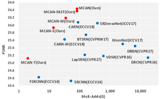
Figure 4: MCAN family (red) compared to others (blue) on $\times 4$ tasks of Urban 100. The multi-adds are calculated in the case of HR is 1280$\times$720.

We use Mult-Adds and the number of parameters to measure the model size. We emphasize on Mult-Adds as it indicates the number of multiply-accumulate operations. By convention, it is normalized on $1280\times 720$ high-resolution images. Further evaluation based on geometric self-ensembling strategy [41] are marked with ‘+’.

Quantitative comparisons with the state-of-the-art methods are listed in Table 1. For fair comparison, we concentrate on models with comparative mult-adds and parameters.

Notably, MCAN outperforms CARN [1] with fewer multi-adds and parameters. The medium-size model MCAN-M [1] achieved better performance than the CARN-M, additionally, it is still on par with CARN with about half of its multi-adds. For short, it surpasses all other listed methods, including MoreMNAS-A [6] and FALSR-A [5] from NAS methods.

The smaller model MCAN-S emulates LapSRN [23] with much fewer parameters. Particularly, it has an average advantage of $0.5$ dB on PSNR over the LapSRN on the $\times 2$ task, and on average, MCAN-S still has an advantage of $0.4$ dB. MCAN-S also behaves better than CARN-M on all tasks with half of its model size. It is worth to note that heavily compressed MCAN-S still exceeds or matches larger models such as VDSR, DRCN, DRRN and MemNet.

The tiny model MCAN-T is meant to be applied under requirements of extreme fast speed. It overtakes FSRCNN [8] on all tasks with the same level of mult-adds.

4.4 Ablation Study

MIM	✘	✔	✘	✔
EFF	✘	✘	✔	✔
Avg. PSNR	29.44	30.25	30.23	30.28

Table 3: Investigations of MIM and EFF. We record the best average PSNR(dB) values of Set5 $\&$ Set14 on $\times 4$ SR task in $10^{5}$ steps.

In this section, we demonstrate the effectiveness of the MIM structure and EFF through ablation study.

Matrix in matrix. We remove the connections between MCACs and also the connections between MCABs. Hence the model comes without intermediate connections. As shown in Table 3, the MIM structure can bring significant improvements, PSNR improves from 29.44 dB to 30.25 dB when such connections are enabled. When EFF is added, PNSR continues to increase from 30.23 dB to 30.28 dB.

Edge feature fusion. We simply eliminate the fusion convolutions connected to MIM and consider the output of the last MCAB as the output of MIM. In this case, the intermediate features acquired by the MIM structure are not directly involved in the reconstruction. In Table 3, we observe that the EFF structure enhances PNSR from 29.44 dB to 30.23 dB. With MIM enabled, PSNR is further promoted from 30.25 dB to 30.28 dB.

5 Conclusion

In this paper, we proposed an accurate and efficient network with matrixed channel attention for the SISR task. Our main idea is to exploit the intermediate features hierarchically through multi-connected channel attention blocks. MCAB then acts as a basic unit that builds up the matrix-in-matrix module. We release three additional efficient models of varied sizes, MCAN-M, MCAN-S, and MCAN-T. Extensive experiments reveal that our MCAN family excel the state-of-the-art models of accordingly similar sizes or even much larger.

To deal with the inefficiency of the sigmoid function on some mobile devices, we benefit from the fast sigmoid to construct MCAN-FAST. The result confirms that MCAN-FAST has only a small loss of precision when compared to MCAN, and it can still achieve better performance with fewer multi-adds and parameters than the state-of-the-art methods.

References

- [1] N. Ahn, B. Kang, and K.-A. Sohn. Fast, accurate, and, lightweight super-resolution with cascading residual network. arXiv preprint arXiv:1803.08664, 2018.
- [2] M. Bevilacqua, A. Roumy, C. Guillemot, and M. L. Alberi-Morel. Low-complexity single-image super-resolution based on nonnegative neighbor embedding. 2012.
- [3] Y. Blau, R. Mechrez, R. Timofte, T. Michaeli, and L. Zelnik-Manor. The 2018 pirm challenge on perceptual image super-resolution. In European Conference on Computer Vision, pages 334–355. Springer, 2018.
- [4] J.-S. Choi and M. Kim. A deep convolutional neural network with selection units for super-resolution. In Computer Vision and Pattern Recognition Workshops (CVPRW), 2017 IEEE Conference on, pages 1150–1156. IEEE, 2017.
- [5] X. Chu, B. Zhang, H. Ma, R. Xu, J. Li, and Q. Li. Fast, accurate and lightweight super-resolution with neural architecture search. arXiv preprint arXiv:1901.07261, 2019.
- [6] X. Chu, B. Zhang, R. Xu, and H. Ma. Multi-objective reinforced evolution in mobile neural architecture search. arXiv preprint arXiv:1901.01074, 2019.
- [7] C. Dong, C. C. Loy, K. He, and X. Tang. Learning a deep convolutional network for image super-resolution. In European conference on computer vision, pages 184–199. Springer, 2014.
- [8] C. Dong, C. C. Loy, and X. Tang. Accelerating the super-resolution convolutional neural network. In European Conference on Computer Vision, pages 391–407. Springer, 2016.
- [9] Y. Fan, H. Shi, J. Yu, D. Liu, W. Han, H. Yu, Z. Wang, X. Wang, and T. S. Huang. Balanced two-stage residual networks for image super-resolution. In Proceedings of the IEEE Conference on Computer Vision and Pattern Recognition Workshops, pages 161–168, 2017.
- [10] G. Georgiou. Parallel Distributed Processing in the Complex Domain. PhD thesis, Tulane, 1992.
- [11] R. Girshick. Fast r-cnn. In Proceedings of the IEEE international conference on computer vision, pages 1440–1448, 2015.
- [12] I. Goodfellow, J. Pouget-Abadie, M. Mirza, B. Xu, D. Warde-Farley, S. Ozair, A. Courville, and Y. Bengio. Generative adversarial nets. In Advances in neural information processing systems, pages 2672–2680, 2014.
- [13] S. Han, H. Mao, and W. J. Dally. Deep compression: Compressing deep neural networks with pruning, trained quantization and huffman coding. arXiv preprint arXiv:1510.00149, 2015.
- [14] K. He, G. Gkioxari, P. Dollár, and R. Girshick. Mask r-cnn. In Proceedings of the IEEE international conference on computer vision, pages 2961–2969, 2017.
- [15] A. Hore and D. Ziou. Image quality metrics: Psnr vs. ssim. In 2010 20th International Conference on Pattern Recognition, pages 2366–2369. IEEE, 2010.
- [16] A. G. Howard, M. Zhu, B. Chen, D. Kalenichenko, W. Wang, T. Weyand, M. Andreetto, and H. Adam. Mobilenets: Efficient convolutional neural networks for mobile vision applications. arXiv preprint arXiv:1704.04861, 2017.
- [17] J.-B. Huang, A. Singh, and N. Ahuja. Single image super-resolution from transformed self-exemplars. In Proceedings of the IEEE Conference on Computer Vision and Pattern Recognition, pages 5197–5206, 2015.
- [18] Z. Hui, X. Wang, and X. Gao. Fast and accurate single image super-resolution via information distillation network. In Proceedings of the IEEE Conference on Computer Vision and Pattern Recognition, pages 723–731, 2018.
- [19] F. N. Iandola, S. Han, M. W. Moskewicz, K. Ashraf, W. J. Dally, and K. Keutzer. Squeezenet: Alexnet-level accuracy with 50x fewer parameters and¡ 0.5 mb model size. arXiv preprint arXiv:1602.07360, 2016.
- [20] J. Kim, J. Kwon Lee, and K. Mu Lee. Accurate image super-resolution using very deep convolutional networks. In Proceedings of the IEEE conference on computer vision and pattern recognition, pages 1646–1654, 2016.
- [21] J. Kim, J. Kwon Lee, and K. Mu Lee. Deeply-recursive convolutional network for image super-resolution. In Proceedings of the IEEE conference on computer vision and pattern recognition, pages 1637–1645, 2016.
- [22] D. P. Kingma and J. Ba. Adam: A method for stochastic optimization. arXiv preprint arXiv:1412.6980, 2014.
- [23] W.-S. Lai, J.-B. Huang, N. Ahuja, and M.-H. Yang. Deep laplacian pyramid networks for fast and accurate superresolution. In IEEE Conference on Computer Vision and Pattern Recognition, volume 2, page 5, 2017.
- [24] C. Ledig, L. Theis, F. Huszár, J. Caballero, A. Cunningham, A. Acosta, A. Aitken, A. Tejani, J. Totz, Z. Wang, et al. Photo-realistic single image super-resolution using a generative adversarial network. arXiv preprint, 2017.
- [25] B. Lim, S. Son, H. Kim, S. Nah, and K. Mu Lee. Enhanced deep residual networks for single image super-resolution. In Proceedings of the IEEE Conference on Computer Vision and Pattern Recognition Workshops, pages 136–144, 2017.
- [26] W. Liu, D. Anguelov, D. Erhan, C. Szegedy, S. Reed, C.-Y. Fu, and A. C. Berg. Ssd: Single shot multibox detector. In European conference on computer vision, pages 21–37. Springer, 2016.
- [27] X. Mao, C. Shen, and Y.-B. Yang. Image restoration using very deep convolutional encoder-decoder networks with symmetric skip connections. In Advances in neural information processing systems, pages 2802–2810, 2016.
- [28] D. Martin, C. Fowlkes, D. Tal, and J. Malik. A database of human segmented natural images and its application to evaluating segmentation algorithms and measuring ecological statistics. In null, page 416. IEEE, 2001.
- [29] V. Nair and G. E. Hinton. Rectified linear units improve restricted boltzmann machines. In Proceedings of the 27th international conference on machine learning (ICML-10), pages 807–814, 2010.
- [30] H. Noh, S. Hong, and B. Han. Learning deconvolution network for semantic segmentation. In Proceedings of the IEEE international conference on computer vision, pages 1520–1528, 2015.
- [31] W. Shi, J. Caballero, F. Huszár, J. Totz, A. P. Aitken, R. Bishop, D. Rueckert, and Z. Wang. Real-time single image and video super-resolution using an efficient sub-pixel convolutional neural network. In Proceedings of the IEEE conference on computer vision and pattern recognition, pages 1874–1883, 2016.
- [32] Y. Tai, J. Yang, and X. Liu. Image super-resolution via deep recursive residual network. In Proceedings of the IEEE Conference on Computer Vision and Pattern Recognition, volume 1, page 5, 2017.
- [33] Y. Tai, J. Yang, X. Liu, and C. Xu. Memnet: A persistent memory network for image restoration. In Proceedings of the IEEE Conference on Computer Vision and Pattern Recognition, pages 4539–4547, 2017.
- [34] R. Timofte, E. Agustsson, L. Van Gool, M.-H. Yang, and L. Zhang. Ntire 2017 challenge on single image super-resolution: Methods and results. In Proceedings of the IEEE Conference on Computer Vision and Pattern Recognition Workshops, pages 114–125, 2017.
- [35] T. Tong, G. Li, X. Liu, and Q. Gao. Image super-resolution using dense skip connections. In Proceedings of the IEEE International Conference on Computer Vision, pages 4799–4807, 2017.
- [36] X. Wang, K. Yu, S. Wu, J. Gu, Y. Liu, C. Dong, Y. Qiao, and C. C. Loy. Esrgan: Enhanced super-resolution generative adversarial networks. In European Conference on Computer Vision, pages 63–79. Springer, 2018.
- [37] Z. Wang, A. C. Bovik, H. R. Sheikh, E. P. Simoncelli, et al. Image quality assessment: from error visibility to structural similarity. IEEE transactions on image processing, 13(4):600–612, 2004.
- [38] J. Yang, J. Wright, T. S. Huang, and Y. Ma. Image super-resolution via sparse representation. IEEE transactions on image processing, 19(11):2861–2873, 2010.
- [39] R. Zhang, P. Isola, and A. A. Efros. Colorful image colorization. In European conference on computer vision, pages 649–666. Springer, 2016.
- [40] X. Zhang, X. Zhou, M. Lin, and J. Sun. Shufflenet: An extremely efficient convolutional neural network for mobile devices. In Proceedings of the IEEE Conference on Computer Vision and Pattern Recognition, pages 6848–6856, 2018.
- [41] Y. Zhang, K. Li, K. Li, L. Wang, B. Zhong, and Y. Fu. Image super-resolution using very deep residual channel attention networks. In European Conference on Computer Vision, pages 294–310. Springer, 2018.
- [42] Y. Zhang, Y. Tian, Y. Kong, B. Zhong, and Y. Fu. Residual dense network for image super-resolution. In Proceedings of the IEEE Conference on Computer Vision and Pattern Recognition, pages 2472–2481, 2018.