A New Lower Bound for Semigroup Orthogonal Range Searching

Abstract

We report the first improvement in the space-time trade-off of lower bounds for the orthogonal range searching problem in the semigroup model, since Chazelle’s result from 1990. This is one of the very fundamental problems in range searching with a long history. Previously, Andrew Yao’s influential result had shown that the problem is already non-trivial in one dimension [13]: using $m$ units of space, the query time $Q(n)$ must be $\Omega(\alpha(m,n)+\frac{n}{m-n+1})$ where $\alpha(\cdot,\cdot)$ is the inverse Ackermann’s function, a very slowly growing function. In $d$ dimensions, Bernard Chazelle [8] proved that the query time must be $Q(n)=\Omega((\log_{\beta}n)^{d-1})$ where $\beta=2m/n$. Chazelle’s lower bound is known to be tight for when space consumption is “high” i.e., $m=\Omega(n\log^{d+\varepsilon}n)$.

We have two main results. The first is a lower bound that shows Chazelle’s lower bound was not tight for “low space”: we prove that we must have $mQ(n)=\Omega(n(\log n\log\log n)^{d-1})$. Our lower bound does not close the gap to the existing data structures, however, our second result is that our analysis is tight. Thus, we believe the gap is in fact natural since lower bounds are proven for idempotent semigroups while the data structures are built for general semigroups and thus they cannot assume (and use) the properties of an idempotent semigroup. As a result, we believe to close the gap one must study lower bounds for non-idempotent semigroups or building data structures for idempotent semigroups. We develope significantly new ideas for both of our results that could be useful in pursuing either of these directions.

1 Introduction

Orthogonal range searching in the semigroup model is one of the most fundamental data structure problems in computational geometry. In the problem, we are given an input set of points to store in a data structure where each point is associated with a weight from a semigroup $\mathscr{G}$ and the goal is to compute the (semigroup) sum of all the weights inside an axis-aligned box given at the query time. Disallowing the “inverse” operation in $\mathscr{G}$ makes the data structure very versatile as it is then applicable to a wide range of situations (from computing weighted sum to computing the maximum or minimum inside the query). In fact, the semigroup variant is the primary way the family of range searching problems are introduced, (see the survey [3]).

Here, we focus only on static data structures. We use the convention that $Q(n)$, the query time, refers to the worst-case number of semigroup additions required to produce the query answer $S(n)$, space, refers to the number of semigroup sums stored by the data structure. By storage, denoted by $S^{+}(n)$, we mean space but not counting the space used by the input, i.e., $S(n)=n+S^{+}(n)$. So we can talk about data structures with sublinear space, e.g., with 0 storage the data structure has to use the input weights only, leading to the worst-case query time of $n$.

1.1 The Previous Results

Orthogonal range searching is a fundamental problem with a very long history. The problem we study is also very interesting from a lower bound point of view where the goal is to understand the fundamental barriers and limitations of performing basic data structure operations. Such a lower bound approach was initiated by Fredman in early 80s and in a series of very influential papers (e.g., see [9, 10, 11]). Among his significant results, was the lower bound [10, 11] that showed a sequence of $n$ insertions, deletions, and queries requires $\Omega(n\log n)$ time to run.

Arguably, the most surprising result of these early efforts was given by Andrew Yao who in 1982 showed that even in one dimension, the static case of the problem contains a very non-trivial, albeit small, barrier. In one dimension, the problem essentially boils down to adding numbers: store an input array $A$ of $n$ numbers in a data structure s.t., we can add up the numbers from $A[i]$ to $A[j]$ for $i$ and $j$ given at the query time. The only restriction is that we should use only additions and not subtractions (otherwise, the problem is easily solved using prefix sums). Yao’s significant result was that answering queries requires $\Omega(\alpha(S(n),n)+n/S^{+}(n))$ additions, where $\alpha(\cdot,\cdot)$ is the inverse Ackermann function. This bound implies that if one insists on using $O(n)$ storage, the query bound cannot be reduced to constant, but even using a miniscule amount of extra storage (e.g., a $\log^{*}\log^{*}n$ factor extra storage) can reduce the query bound to constant. Furthermore, using a bit less than $n$ storage, e.g., by a $\log^{*}\log^{*}n$ factor, will once again yield a more natural (and optimal) bound of $n/S^{+}(n)$. Despite its strangeness, it turns out there are data structures that can match the exact lower bound (see also [4]). After Tarjan’s famous result on the union-find problem [12], this was the second independent appearance of the inverse Ackermann function in the history of algorithms and data structures.

Despite the previous attempts, the problem is still open even in two dimensions. At the moment, using range trees [6, 7] on the 1D structures is the only way to get two or higher dimensional results. In 2D for instance, we can have $S^{+}(n)=O(n/\log n)$ with query bound $Q(n)=O(\log^{3}n)$, or $S^{+}(n)=O(n)$ with query bound $Q(n)=O(\log^{2}n)$, or $S^{+}(n)=O(n\log n)$ with query bound $O(\alpha(cn,n)\log n)$, for any constant $c$. In general and in $d$ dimensions, we can build a structure with $S^{+}(n)=O(n\log^{d-1}n)$ units of storage and with $Q(n)=O(\alpha(cn,n)\log^{d-1}n)$ query bound, for any constant $c$. We can reduce the space complexity by any factor $t$ by increasing the query bound by another factor $t$. Also, strangely, if $t$ is asymptotically larger than $\alpha(n,n)$, then the inverse Ackermann term in the query bound disappears. Nonetheless, a surprising result of Chazelle [8] shows that the reverse is not true: the query bound must obey $Q(n)=\Omega((\log_{S(n)/n}n)^{d-1})$ which implies using polylogarithmic extra storage only reduces the query bound by a $(\log\log n)^{d-1}$ factor. Once again, using range tree with large fan out, one can build a data structure that uses $O(n\log^{2d-2+\varepsilon}n)$ storage, for any positive constant $\varepsilon$, and achieves the query bound of $O((\log_{\log n}n)^{d-1})$. This, however leaves a very natural and important open problem: Is Chazelle’s lower bound the only barrier? Is it possible to achieve $O(n)$ space and $O(\log^{d-1}n)$ query time?

Idempotence and random point sets.

A semigroup is idempotent if for every $x\in\mathscr{G}$, we have $x+x=x$. All the previous lower bounds are in fact valid for idempotent semigroups. Furthermore, Chazelle’s lower bound uses a uniform (or randomly placed) set of points which shows the lower bound does not require pathological or fragile input constructions. Furthermore, his lower bound also holds for dominance ranges, i.e., $d$-dimensional boxes in the form of $(-\infty,a_{1}]\times\dots\times(-\infty,a_{d}]$. These little perks result in a very satisfying statement: problem is still difficult even when $\mathscr{G}$ is “nice” (idempotent), and when the point set is “nice” (uniformly placed) and when the queries are simple (“dominance queries”).

1.2 Our Results

We show that for any data structure that uses $S^{+}(n)$ storage and has query bound of $Q(n)$, we must have $S^{+}(n)\cdot Q(n)=\Omega(n(\log n\log\log n)^{d-1})$. This is the first improvement to the storage-time trade-off curve for the problem since Chazelle’s result in 1990. It also shows that Chazelle’s lower bound is not the only barrier. Observe that our lower bound is strong at a different corner of parameter space compared to Chazelle’s: ours is strongest when storage is small whereas Chazelle’s is strongest when the storage is large. Furthermore, we also keep most of the desirable properties of Chazelle’s lower bound: our lower bound also holds for idempotent semigroups and uniformly placed point sets. However, we have to consider more complicated queries than just dominance queries which ties to our second main result. We show that our analysis is tight: given a “uniformly placed” point set and an idempotent semigroup $\mathscr{G}$, we can construct a data structure that uses $O(n)$ storage and has the query bound of $O((\log n\log\log n)^{d-1})$. As a corollary, we provide an almost complete understanding of orthogonal range searching queries with respect to a uniformly placed point set in an idempotent semigroup.

Challenges.

Our results and specially our lower bound require significantly new ideas. To surpass Chazelle’s lower bound, we need to go beyond dominance queries which requires wrestling with complications that ideas such as range trees can introduce. Furthermore, in our case, the data structure can actually improve the query time by a factor $f$ by spending a factor $f$ extra space. This means, we are extremely sensitive to how the data structure can “use” its space. As a result, we need to capture the limits of how intelligently the data structure can spend its budge of “space” throughout various subproblems.

Implications.

It is natural to conjecture that the uniformly randomly placed point set should be the most difficult point set for orthogonal queries. Because of this, we conjecture that our lower bounds are almost tight. This opens up a few very interesting open problems. See Section 5.

2 Preliminaries

The Model of Computation.

Let $P$ be an input set of $n$ points with weights from a semigroup $\mathscr{G}$. Our model of computation is the same as the one used by the previous lower bounds, e.g., [8]. There has been quite some work dedicated to building a proper model for lower bounds in the semigroup model. We will not delve into those details and we only mention the final consequences of the efforts. The data structure stores a number of sums where each sum $s$ is the sum of the weights of a subset $s_{P}\subset P$. With a slight abuse of the notation, we will use $s$ to refer both to the sum as well as to the subset $s_{P}$. The number of stored sums is the space complexity of the data structure. If a sum contains only one point, then we call it a singleton and we use $S^{+}(n)$ to denote the storage occupied by sums that are not singletons. Now, consider a query range $r$ containing a subset $r_{P}=r\bigcap P$. The query algorithm must find $k$ stored subsets $s_{1},\dots,s_{k}$ such that $r_{P}=\cup_{i=1}^{k}s_{i}$. For a given query $r$, the smallest such integer $k$ is the query bound of the query. The query bound of the data structure is the worst-case query bound of any query. Observe that the data structure does not disallow covering any point more than once and in fact, for idempotent semigroups this poses no problem. All the known lower bounds work in this way, i.e., they allow covering a point inside the query multiple times. However, if the semigroup is not idempotent, then covering a point more than once could lead to incorrect results. Since data structures work for general semigroups, they ensure that $s_{1},\dots,s_{k}$ are disjoint.

Definitions and Notations.

A $d$-dimensional dominance query is determined by one point $(x_{1},\dots,x_{d})$ and it is defined as $(-\infty,x_{1}]\times\dots\times(-\infty,x_{d}]$.

Definition 2.1.

We call a set $P\subset\mathbb{R}^{d}$ well-distributed if the following properties hold: (i) $P$ is contained in the $d$-dimensional unit cube. (ii) The volume of any rectangle that contains $k\geq 2$ points of $P$ is at least $\varepsilon_{d}k/|P|$ for some constant $\varepsilon_{d}$ that only depends on the dimension. (iii) Any rectangle that has volume $v$, contains at most $\lceil v|P|/\varepsilon_{d}\rceil$ points of $P$.

Lemma 1.

[1, 8, 2] For any constant $d$ and any given value of $n$, there exists a well-distributed point set in $\mathbb{R}^{d}$ containing $\Theta(n)$ points.

3 The Lower Bound

This section is devoted to the proof of our main theorem which is the following.

Theorem 3.1.

If $P$ is a well-distributed point set of $n$ points in $\mathbb{R}^{d}$, any data structure that uses $S^{+}(n)$ storage, and answers $(2d-1)$-sided queries in $Q(n)$ query bound requires that $S^{+}(n)\cdot Q(n)=\Omega(n(\log n\log\log n)^{d-1})$.

Let $\mathcal{Q}$ be the unit cube in $\mathbb{R}^{d}$. Throughout this section, the input point set is a set $P$ of $n$ well-distributed points in $\mathcal{Q}$. Let $\mathscr{D}$ be a data structure that answers semigroup orthogonal range searching queries on $P$.

3.1 Definitions and Set up

We consider queries that have two boundaries in dimensions 1 to $d-1$ but only have an upper bound in dimension $d$. For simplicity, we rename the axes such that the $d$-th axis is denoted by $Y$ and the first $d-1$ axes are denoted by $X_{1},\dots,X_{d-1}$. Thus, each query is in the form of $[x^{\prime}_{1},x_{1}]\times\dots[x^{\prime}_{d-1},x_{d-1}]\times(-\infty,y]$. The point $(x_{1},\dots,x_{d-1},y)$ is defined as the dot of $q$ and is denoted by $\mbox{Dot}(q)$. For every $1\leq i\leq d-1$, the line segment that connects $\mbox{Dot}(q)$ to the point $(x_{1},\dots,x_{i-1},x^{\prime}_{i},x_{i+1},\dots,x_{d-1},y)$ is called the $i$-th marker of $q$ and it is denoted by $t_{i}(s)$.

The tree $T_{i}$.

For each dimension $i=1,\dots,d-1$, we define a balanced binary tree $T_{i}$ of height $h=\log n$ as follows. Informally, we cut $\mathcal{Q}$ into $2^{h}$ congruent boxes with hyperplanes perpendicular to axis $X_{i}$ which form the leaves of $T_{i}$. To be more specific, every node in $T_{i}$ is assigned a box $r(v)\subset\mathcal{Q}$. The root of $T_{i}$ is assumed to have depth $0$ and it is assigned $\mathcal{Q}$. For every node $v$, we divide $r(v)$ into two congruent “left” and “right” boxes with a hyperplane $\ell(v)$, perpendicular to $X_{i}$ axis. The left box is assigned to left child of $v$ and similarly the right box is assigned to the right child of $v$. We do not do this if $r(v)$ has volume less than $1/n$; these nodes become the leaves of $T$. Observe that all trees $T_{i}$, $1\leq i\leq d-1$ have the same height $h$. The volume of $r(v)$ for a node $v$ at depth $j$ is $2^{-j}$.

Embedding the problem in $\mathbb{R}^{2d-1}$.

The next idea is to embed our problem in $\mathbb{R}^{2d-1}$. Consistent with the previous notation, the first $d$ axes are $X_{1},\dots,X_{d-1}$ and $Y$. We label the next axis $Z_{1},\dots,Z_{d-1}$. We now represent $T_{i}$ geometrically as follows. Consider $h$ the height of $T_{i}$. For each $i$, $1\leq i\leq d-1$, we now define a representative diagram $\Gamma_{i}$ which is a axis-aligned decomposition of the unit (planar) square $Q_{i}$ in a coordinate system where the horizontal axis is $X_{i}$ and the vertical axis is $Z_{i}$. As the first step of the decomposition, cut $Q_{i}$ into $h$ equal-sized sub-rectangles using $h-1$ horizontal lines. Next, we will further divide each sub-rectangle into small regions and we will assign every node $v$ of $T_{i}$ to one of these regions. This is done as follows. The root $v$ of $T_{i}$ is assigned the topmost sub-rectangle as its region, $\gamma(v)$. Assume $v$ is assigned a rectangle $\gamma(v)$ as its region. We create a vertical cut starting from the middle point of the lower boundary of $\gamma(v)$ all the way down to the bottom of the rectangle $Q_{i}$. The children of $v$ are assigned to the two rectangles that lie immediately below $\gamma(v)$. See Figure 1.

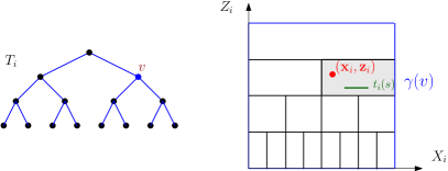
Figure 1: A tree and its representative diagram. The region of a node $v$ is highlighted in grey.

Placing the Sums.

Consider a semigroup sum $s$ stored by the data structure $\mathscr{D}$. Our lower bound will also apply to semigroups that are idempotent which means without loss of generality, we can assume that our semigroup is idempotent. As a result, we can assume that each semigroup sum $s$ stored by the data structure has the same shape as the query. Let $b(s)$ be the smallest box that is unbounded from below (along the $Y$ axis) that contains all the points of $s$. If $s$ does not include a point, $p$, inside $b(s)$, we can just $p$ to $s$. Any query that can use $s$ must contain the box $b(s)$ which means adding $p$ to $s$ can only improve things. Each sum $s$ is placed in one node of $T_{i}$ for every $1\leq i\leq d-1$. The details of this placement are as follows.

A node $v_{i}$ in $T_{i}$ stores any sum $s$ such that the $i$-th marker of $s$, $t_{i}(s)$, intersects $\ell(v_{i})$ with $v$ being the highest node with this property. Geometrically, this is equivalent to the following: we place $s$ at a node $v$ if $\gamma(v)$ is the lowest region that fully contains the segment $t_{i}(s)$ (or to be precise, the projection of $t_{i}(s)$ onto the $Z_{i}X_{i}$ plane). For example, in Figure 1(right), the sum $s$ is placed at $v$ in $T_{i}$ since $t_{i}(s)$, the green line segment, is completely inside $\gamma(v)$ with $v$ being the lowest node of this property. Remember that $s$ is placed at some node in each tree $T_{i}$, $1\leq i\leq d-1$ (i.e., it is placed $d-1$ times in total).

Notations and difficult queries.

We will adopt the convention that random variables are denoted with bold math font. The difficult query is a $2d-1$ sided query chosen randomly as follows. The query is defined as $[\mathbf{x}^{\prime}_{1},\mathbf{x}_{1}]\times\dots\times[\mathbf{x}^{\prime}_{d-1},\mathbf{x}_{d-1}]\times(-\infty,\mathbf{y}]$ where $\mathbf{x}^{\prime}_{i},\mathbf{x}_{i}$ and $\mathbf{y}$ are also random variables (to be described). $\mathbf{y}$ is chosen uniformly in $[0,1]$. To choose the remaining coordinates, we do the following. We place a random point $(\mathbf{x}_{i},\mathbf{z}_{i})$ uniformly inside the representative plane $\Gamma_{i}$ (i.e., choose $\mathbf{x}_{i}$ and $\mathbf{z}_{i}$ uniformly in $[0,1]$). Let $\mathbf{v}_{i}$ be the random variable denoting the node in $T_{i}$ s.t., region $\gamma(\mathbf{v}_{i})$ contains the point $(\mathbf{x}_{i},\mathbf{z}_{i})$. $\mathbf{x}^{\prime}_{i}$ is the $X_{i}$-coordinate of the left boundary of $\gamma(\mathbf{v}_{i})$. Let $\boldsymbol{\ell}_{i}$ be the depth of $\mathbf{v}_{i}$ in $T_{i}$. We denote the point $(\mathbf{x}_{1},\dots,\mathbf{x}_{d-1},\mathbf{y})$ by $\mathbf{q}$ and denote the $2d-1$ sided query by $\mbox{Dom}_{\mathbf{v}_{1},\ldots,\mathbf{v}_{d-1}}(\mathbf{q})$. See Figure 1(right). Note that a query $\mbox{Dom}_{v_{1},\ldots,v_{d-1}}(q)$ is equivalent to a dominance query defined by point $q$ in $r(v_{1})\cap\dots\cap r(v_{d-1})$. To simplify the presentation and to stop redefining these concepts, we will reserve the notations introduced in this paragraph to only represent the concepts introduced here.

Observation 1.

A necessary condition for being able to use a sum $s$ to answer $\mbox{Dom}_{v_{1},\dots,v_{d-1}}(q)$ is that $s$ is stored at the subtree of $v_{i}$, for every $1\leq i\leq d-1$.

Proof 3.2.

Due to how we have placed the sums, the sums stored at the ancestors of $v_{i}$ contain at least one point that lies outside $r(v_{i})$ and since $\mbox{Dom}(q)$ is entirely contained inside $r(v_{i})$ those sums cannot be used to answer the query.

Subproblems.

Consider a query $\mbox{Dom}(q)=\mbox{Dom}_{v_{1},\dots,v_{d-1}}(q)$. We now define subproblems of $\mbox{Dom}(q)$. A subproblem is represented by an array of $d-1$ integral indices ${\rm AJ}=(j_{1},\dots,j_{d-1})$ and it is denoted as ${\rm AJ}$-subproblem. The state of ${\rm AJ}$-subproblem of a query $\mbox{Dom}_{v_{1},\ldots,v_{d-1}}(q)$ could either be undefined, or it could refer to covering a particular subset of points inside the query. In particular, given $\mbox{Dom}(q)$, a ${\rm AJ}$-subproblem is undefined if for some $1\leq i\leq d-1$, there is no node $u_{i}\in T_{i}$ with the following properties: $u_{i}$ has depth $\ell_{i}+j_{i}$, $u_{i}$ has a right sibling $u^{\prime}_{i}$ with $r(u^{\prime}_{i})$ containing the query point $q$. See Figure 2. However, if such nodes $u_{i}$ exist for all $1\leq i\leq d-1$, then the ${\rm AJ}$-subproblem of $\mbox{Dom}(q)$ is well-defined and it refers to the problem of covering all the points inside the region $\mbox{Dom}(q)\cap r(u_{1})\cap\dots\cap r(u_{d-1})$; observe that this is equivalent to covering all the points inside the region $r(u_{1})\cap\dots\cap r(u_{d-1})$ that have $Y$-coordinate at most $y$. Further observe that for $u_{i}$ to exist in $T_{i}$, it needs to pass two checks: (check I) $\ell_{i}+j_{i}\leq h$ as otherwise, there are no nodes with depth $\ell_{i}+j_{i}$ and (check II) a node $u_{i}$ at depth $\ell_{i}+j_{i}$ has a right sibling $u^{\prime}_{i}$ with $r(u^{\prime}_{i})$ containing $q$. The nodes $u_{1},\dots,u_{d-1}$ are called the defining nodes of the ${\rm AJ}$-subproblem. Thus, the random variable $\mathbf{v}_{i}$ defines the random variable $\mathbf{u}_{i}$ where $\mathbf{u}_{i}$ could be either undefined or it could be a node in $T_{i}$. Clearly, the distribution of $\mathbf{u}_{i}$ is independent of the distributions of $\mathbf{u}_{j}$ and $\mathbf{v}_{j}$ for $i\not=j$ as $\mathbf{u}_{i}$ only depends on $\mathbf{v}_{i}$.

Observation 2.

Consider a well-defined ${\rm AJ}=(j_{1},\dots,j_{d-1})$ subproblem of a query $\mbox{Dom}_{v_{1},\dots,v_{d-1}}(q)$ and its defining nodes $u_{1},\dots,u_{d-1}$. To solve the ${\rm AJ}$-subproblem (i.e., to cover the points inside the subproblem), the data structure can use a sum $s$ only if for every $1\leq i\leq d-1$, we either have case (i) where $s$ is stored at ancestors of $u_{i}$ but not the ancestors of $v_{i}$ or case (ii) where $s$ is stored at the subtree of $u_{i}$. If a sum $s$ violates one of these two conditions for some $i$, then it cannot be used to answer the ${\rm AJ}$-subproblem. See Figure 2.

Proof 3.3.

First we use Observation 1. $s$ must be stored at the subtree of $v_{i}$. Let $w$ be the node that stores $s$. If $w$ is in the subtree of $u_{i}$, then we are done. Otherwise, let $v^{\prime}$ be the least common ancestor of $u_{i}$ and $w$. If $v^{\prime}=w$ then we are done again but otherwise, $u$ belongs to the subtree of one child of $v^{\prime}$ while $w$ belongs to the subtree of the other child of $v^{\prime}$. By our placement rules, this implies that $s$ is entirely outside $r(u_{i})$ and thus it cannot be used to answer the ${\rm AJ}$-subproblem.

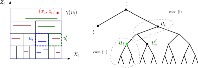
Figure 2: $u_{i}$ is a defining node. The blue line segments correspond to $t_{i}(s)$ of a sum $s$ that is placed in the subtree of $u_{i}$. The green ones correspond to those placed at ancestors of $u_{i}$ but not at ancestors of $v_{i}$. The red ones correspond to sums that cannot be used to answer the subproblem.

3.2 The Main Lemma

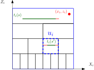
Figure 3: The extensions of two sums that can be used to answer a subproblem.

In this subsection, we prove a main lemma which is the heart of our lower bound proof. To describe this lemma, we first need the following notations. Consider a well-defined ${\rm AJ}$-subproblem of a query $\mbox{Dom}_{v_{1},\ldots,v_{d-1}}(q)$ where $j_{i}\leq\frac{h}{2}$ for $1\leq i\leq d-1$. As discussed, this subproblem corresponds to covering all the points in the region $r(u_{1})\cap\cdots\cap r(u_{d-1})$ whose $Y$-coordinate is below $y$, the $Y$-coordinate of point $q$; thus, the ${\rm AJ}$-subproblem of the query can be represented as the problem of covering all the points inside the box $[a_{1},b_{1}]\times\cdots\times[a_{d-1},b_{d-1}]\times(-\infty,y]$ where $a_{i}$ and $b_{i}$ correspond to the left and the right boundaries of the slab $r(u_{i})$. Let $0<\lambda$ be a parameter. Consider the region $[a_{1},b_{1}]\times\cdots\times[a_{d-1},b_{d-1}]\times[y-\beta,y]$ in which $\beta$ is chosen such that the region contains $\lambda$ points; as our pointset is well-distributed, this implies that the volume of the region is $\Theta(\lambda/n)$. We call this region the $\lambda$-top box. The $\lambda$-top, denoted by $\mbox{Top}({\rm AJ},\lambda)$, is then the problem of covering all the points inside the $\lambda$-top box of the ${\rm AJ}$-subproblem. With a slight abuse of the notation, we will use $\mbox{Top}({\rm AJ},\lambda)$ to refer also to the set of points inside the $\lambda$-top box. If there are not enough points in the $\lambda$-top box, the $\lambda$-top is undefined, otherwise, it is well-defined. These of course also depend on the query but we will not write the dependency on the query as it will clutter the notation. Furthermore, observe that when the query is random, then $\mbox{Top}({\rm AJ},\lambda)$ becomes a random variable which is either undefined or it is some subset of points.

Extensions of sums.

Due to technical issues, we slightly extend the number of points each sum covers. Consider a sum $s$ stored at a subtree of $v_{i}$ such that $s$ can be used to answer the ${\rm AJ}$-subproblem. By Observation 1, $s$ is either placed at the subtree of $u_{i}$ or on the path connecting $v_{i}$ to $u_{i}$. We extend the $X_{i}$ range of the sum $s$ (i.e., the projection of $s$ on the $X_{i}$) to include the left and the right boundary of the node $u_{i}$ along the $X_{i}$-dimension. We do this for all $d-1$ first dimensions to obtain an extension $e(s)$ of sum $s$. We allow the data structure to cover any point in $e(s)$ using $s$.

Lemma 2.

[The Main Lemma] Consider a ${\rm AJ}=(j_{1},\dots,j_{d-1})$ subproblem of a random query $\mbox{Dom}_{\mathbf{v}_{1},\dots,\mathbf{v}_{d-1}}(\mathbf{q})$, for $1\leq j_{i}\leq h/2$. Let $\lambda=\frac{\delta h^{d-1}}{j_{1}j_{2}\dots j_{d-1}}\cdot\frac{n}{S^{+}(\mathcal{A})}$ where $\delta$ is a small enough constant and $S^{+}(\mathcal{A})$ is the storage of the data structure. Let $\mathbf{S}_{\rm AJ}$ be the set of sums $s$ such that (i) $s$ is contained inside the query $\mbox{Dom}_{\mathbf{v}_{1},\dots,\mathbf{v}_{d-1}}(\mathbf{q})$, and (ii) $e(s)$ covers at least $C$ points from $\mbox{Top}({\rm AJ},\lambda)$, meaning, $|e(s)\cap\mbox{Top}({\rm AJ},\lambda)|\geq C$ where $C$ is a large enough constant.

With $\Omega(1)$ probability, the ${\rm AJ}$-subproblem and the $\mbox{Top}({\rm AJ},\lambda)$ are well-defined. Furthermore conditioned on both of these being well-defined, with probability $1-O(\sqrt{\delta/\varepsilon_{d}})$, the nodes $\mathbf{v}_{1},\cdots,\mathbf{v}_{d-1}$ will be sampled as nodes $v_{1},\cdots,v_{d-1}$, s.t., the following holds: $\mathbb{E}[\sum_{s\in\mathbf{S}_{\rm AJ}}|e(s)\cap\mbox{Top}({\rm AJ},\lambda)|]<\frac{|\mbox{Top}({\rm AJ},\lambda)|}{C^{\prime}}$ where the expectation is over the random choices of $\mathbf{y}$ and $C^{\prime}$ is another large constant.

Let us give some intuition on what this lemma says and why it is critical for our lower bound. For simplicity assume $S^{+}(\mathcal{A})=n$ and assume we sample $\mathbf{v}_{1},\cdots,\mathbf{v}_{d-1}$ as the first step, and and then sample $\mathbf{y}$ as the last step. The above lemma implies that if we focus on one particular subproblem, the sums in the data structure cannot cover too many points; to see this consider the following. The lemma first says that after the first step, with positive constant probability, ${\rm AJ}$-subproblem and $\mbox{Top}({\rm AJ},\lambda)$ are well-defined. Furthermore, here is a very high chance that our random choices will “lock us” in a “doomed” state, after sampling $v_{1},\cdots,v_{d-1}$. Then, when considering the random choices of $\mathbf{y}$, sums that cover at least $C$ points in total cover a very small fraction of the points. As a result, we will need $\Omega(\lambda/C)=\Omega(\frac{\delta\log^{d-1}n}{Cj_{1}j_{2}\dots j_{d-1}})$ sums to cover the points inside the $\lambda$-top of the subproblem. Summing these values over all possible subproblems, $j_{i},1\leq j_{i}\leq h/2$, $1\leq i\leq d-1$ will create a lot of Harmonic sums of the type $\sum_{x=1}^{h/2}x=O(\log\log n)$ which will eventually lead to our lower bound. In particular, we will have $\sum_{j_{i},1\leq j_{i}\leq h/2}\Omega(\frac{h^{d-1}}{j_{1}j_{2}\dots j_{d-1}})=(\log n\log\log n)^{d-1}.$ There is however, one very big technical issue that we will deal with later: a sum can cover very few points from each subproblem but from very many subproblems! Without solving this technical issue, we only get the bound $\max_{j_{i},1\leq j_{i}\leq h/2}\Omega(\frac{h^{d-1}}{j_{1}j_{2}\dots j_{d-1}})=(\log n)^{d-1}$ which offers no improvements over Chazelle’s lower bound. Thus, while solving this technical issue is important, nonetheless, it is clear that the lemma we will prove in this section is also very critical.

As this subsection is devoted to the proof of the above lemma, we will assume that we are considering a fixed ${\rm AJ}$-subproblem and thus the indices $j_{1},\ldots,j_{d-1}$ are fixed.

3.2.1 Notation and Setup

By Observation 2, only a particular set of sums can be used to answer the ${\rm AJ}$-subproblem of a query. Consider a sum $s$ that can be used to answer the subproblem of some query. By the observation, we must have that $s$ must either satisfy case (i) or case (ii) for every tree $T_{i}$, $1\leq i\leq d-1$. Over all indices $i$, $1\leq i\leq d-1$, they describe $2^{d-1}=O(1)$ different cases. This means that we can partition $\mathbf{S}_{\rm AJ}$ into $2^{d-1}$ different equivalent classes s.t., for any two sums $s_{1}$ and $s_{2}$ in an equivalent class, either they both satisfy case (i) or they both satisfy case (ii) in Observation 2 and for any dimension $i$. Since $2^{d-1}$ is a constant, it suffices to show that our lemma holds when only considering sums of particular equivalent class. In particular, let $S^{\prime}_{\rm AJ}$ be the subset of eligible sums that all belong to one equivalent class. Now, it suffices to show that $\mathbb{E}[\sum_{s\in S^{\prime}_{\rm AJ}}|e(s)\cap\mbox{Top}({\rm AJ},\lambda)|]<\frac{|\mbox{Top}({\rm AJ},\lambda)|}{2^{d}C^{\prime}}$. since summing these over all $2^{d-1}$ equivalent classes will yield the lemma. Furthermore, w.l.o.g and by renaming the $X$-axes, we can assume that there exists a fixed value $t$, $0\leq t\leq d-1$, such that for every sum $s\in S^{\prime}_{\rm AJ}$, for dimensions $1\leq i\leq t$, $s$ satisfies case (i) in $T_{i}$ and for $t<i\leq d-1$, $s$ is within case (ii). Note that if $t=0$, then it implies that we have no instances of case (i) and for $t=d-1$ we have no instances of case (ii).

The probability distribution of subproblems.

To proceed, we need to understand the distribution of the subproblems. This is done by the following observation.

Observation 3.

Consider a ${\rm AJ}=(j_{1},\dots,j_{d-1})$ subproblem of a random query $\mbox{Dom}_{\mathbf{v}_{1},\dots,\mathbf{v}_{d-1}}(\mathbf{q})$ defined by random variables $\mathbf{u}_{1},\dots,\mathbf{u}_{d-1}$. We can make the following observations. (i) the distribution of the random variable $j_{i}+\boldsymbol{\ell}_{i}$ is uniform among the integers $j_{i}+1,\dots,h+j_{i}$. (ii) With probability $j_{i}/h$, $\mathbf{u}_{i}$ will be undefined because it fails (Check I). (iii) If (Check I) does not fail for $\mathbf{u}_{i}$, there is exactly 0.5 probability that $\mathbf{u}_{i}$ is undefined. (iv) For a fixed $j_{i}$, the probability distribution, $\mu_{i}$, of $\mathbf{u}_{i}$ is as follows: with probability $1-\frac{1-j_{i}/h}{2}$, $\mathbf{u}_{i}$ is undefined. Otherwise, $\mathbf{u}_{i}$ is a node in $T_{i}$ sampled in the following way: sample a random integer (depth) $\boldsymbol{\ell}^{\prime}$ uniformly among integers in $j_{i}+1,\dots,h$ and select a random node uniformly among all the nodes at depth $\boldsymbol{\ell}^{\prime}$ that have a right sibling.

Proof 3.4.

(i) follows directly from our definition: first, note that each coordinate of the query point is chosen independently of other coordinates, and second, $\mathbf{v}_{i}$ is sampled by placing a random point inside $T_{i}$ which by construction implies the depth $\boldsymbol{\ell}_{i}$ of $\mathbf{v}_{i}$ is a uniform random integer in $[h]$. (ii) This directly follows from (i): with probability $j_{i}/h$, the random variable $\boldsymbol{\ell}_{i}$ is larger than $h-j_{i}$ which implies we fail Check I. (iii) We need to make two observations: one is that $j_{i}+\boldsymbol{\ell}_{i}\geq 2$ at all times since $j_{i}\geq 1$ and second that at any depth of $T_{i}$, except for the top level (i.e., the root), exactly half the nodes have a right sibling. (iv) This is simply a consequence of parts (i-iii).

Partial Queries.

Observe that w.l.o.g., we can assume that we first generate the dimensions $1$ to $t$ of the query, and then the dimensions $t+1$ to $d-1$ of the query, and then the value $\mathbf{y}$. A partial query is one where only the dimensions $1$ to $t$ have been generated. This is equivalent to only sampling $t$ random points $(\mathbf{x}_{i},\mathbf{z}_{i})$ for $1\leq i\leq t$. To be more specific, assume we have set $\mathbf{v}_{i}=v_{i}$, for $1\leq i\leq t$ where each $v_{i}$ is a node in $T_{i}$. Then, the partial query is equivalent to the random query $\mbox{Dom}_{v_{1},\dots,v_{t},\mathbf{v}_{t+1},\dots,\mathbf{v}_{d-1}}(\mathbf{q})$ and in which the first $t$ coordinates of $\mathbf{q}$ are known (not random). Thus, we can still talk about the ${\rm AJ}$-subproblem of a partial query; it could be that the ${\rm AJ}$-subproblem is already known to be undefined (this happens when one of the nodes $u_{i}$, $1\leq i\leq t$ is known to be undefined) but otherwise, it is defined by defining nodes $u_{1},\dots,u_{t}$ and the random variables $\mathbf{u}_{t+1},\dots,\mathbf{u}_{d-1}$; these latter random variables could later turn out to be undefined and thus rendering the ${\rm AJ}$-subproblem of the query undefined.

After sampling a partial query, we can then talk about eligible sums: a sum $s$ is eligible if it could potentially be used to answer the ${\rm AJ}$-subproblem once the full query has been generated. Note that the emphasis is on answering the ${\rm AJ}$-subproblem. This means, there are multiple ways for a sum to be ineligible: if ${\rm AJ}$-subproblem is already known to be undefined then there are no eligible sums. Otherwise, the defining nodes $u_{1},\cdots,u_{t}$ are well-defined. In this case, if it is already known that $s$ is outside the query, or it is already known that $s$ cannot cover any points from the ${\rm AJ}$-subproblem then $s$ becomes ineligible. Final and the most important case of ineligibility is when $s$ is placed at a node $w_{i}$ which is a descendant of node $u_{i}\in T_{i}$ for some $1\leq i\leq t$. If this happens, even though $s$ can be potentially used to answer the ${\rm AJ}$-subproblem, it can do so from a different equivalent class, as the reader should remember that we only consider sums that are stored in the path that connects $u_{i}$ to $v_{i}$ for $1\leq i\leq t$. If a sum passes all these, then it is eligible. Clearly, once the final query is generated, the set $S^{\prime}_{\rm AJ}$ is going to be a subset of the eligible sums.

Definition 3.5.

Given a partial query $\mbox{Dom}_{v_{1},\dots,v_{t},\mathbf{v}_{t+1},\dots,\mathbf{v}_{d-1}}(\mathbf{q})$, and considering a fixed ${\rm AJ}$-subproblem, we define the potential function $\Phi_{v_{1},\dots,v_{t}}$ to be the number of eligible sums.

Lemma 3.

We have

$$\mathbb{E}(\Phi_{\mathbf{v}_{1},\dots,\mathbf{v}_{t}}\cdot\prod_{i=1}^{t}\frac{h2^{\boldsymbol{\ell}_{i}+j_{i}}}{j_{i}})\leq O(S^{+}(\mathscr{D})).$$

To prove the above lemma, we need the following definitions and observations.

Definition 3.6.

Consider the ${\rm AJ}$-subproblem for a partial query $\mbox{Dom}_{v_{1},\dots,v_{t},\mathbf{v}_{t+1},\dots,\mathbf{v}_{d-1}}(\mathbf{q})$ together with corresponding nodes $u_{1},\dots,u_{t}$. In the representative diagram $\Gamma_{i}$, the Type I region of $u_{i}$ is defined as a rectangular region whose bottom and left boundary are the same the bottom and the left boundary of $\gamma(u_{i})$, its right boundary is the right boundary of $\gamma(u^{\prime}_{i})$, and its top boundary is the top boundary of $\gamma(v)$. We denote this region by $t_{I}(u_{i})$. See Figure 4.

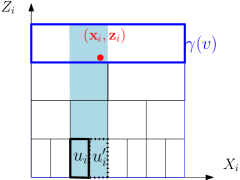
Figure 4: The type I region of $u_{i}$ is highlited.

Observation 4.

Consider a partial query $\mbox{Dom}_{v_{1},\dots,v_{t},\mathbf{v}_{t+1},\dots,\mathbf{v}_{d-1}}(\mathbf{q})$ and assume the nodes $u_{1},\dots,u_{t}$ that correspond to the ${\rm AJ}$-subproblem of the query exist. A necessary condition for a sum $s$ to be eligible is that $\mbox{Dot}_{i}(s)$ must lie inside $t_{I}(u_{i})$ for $1\leq i\leq t$.

Proof 3.7.

As $u_{i}$ is a defined node in $T_{i}$, it means that we can identify the node $u^{\prime}_{i}$, the sibling of $u_{i}$, and the node $v_{i}$, the node at depth $\ell_{i}^{\prime}-j_{i}$ that is the ancestor of $u_{i}$. If $\mbox{Dot}_{i}(s)$ is not inside $t_{I}(u_{i})$, then we have a few cases:

• $\mbox{Dot}_{i}(s)$ is to the left of the left boundary of $t_{I}(u_{i})$: well in this case, $s$ cannot contain any point from the points in the subtree of $u_{i}$ so clearly it cannot be used to answer the ${\rm AJ}$-subproblem.

• $\mbox{Dot}_{i}(s)$ is to the right of the right boundary of $t_{I}(u_{i})$: Observe that $u_{i}$ satisfies Check II, which means the $i$-th coordinates of the query is within the $i$-th coordinates of $u^{\prime}_{i}$. Thus, in this case, it follows that $\mbox{Dot}_{i}(s)$ is outside the query region and so cannot be used to answer the query.

• $\mbox{Dot}_{i}(s)$ is below the lower boundary of $t_{I}(u_{i})$: This violates the assumption that $s$ is an eligible sum. In particular, this implies that $s$ is stored at the subtree of $u_{i}$ in $T_{i}$.

• $\mbox{Dot}_{i}(s)$ is above the top boundary of $t_{I}(u_{i})$: This violates Observation 1 as it implies $s$ is stored at a node which is not in the subtree of $v_{i}$.

We now return to the proof of the Lemma 3. See 3

Proof 3.8.

If the query does not have a ${\rm AJ}$-subproblem then the potential is zero and thus there is nothing left to prove. So in the rest of the proof, we will assume ${\rm AJ}$-subproblem is defined.

Consider an eligible sum $s$ and assume $s$ has been placed at nodes $w_{i}$ of $T_{i}$, for $1\leq i\leq t$. Let $a_{i}$ be the depth of $w_{i}$. We now focus on the distribution of the random variables $\mathbf{u}_{i}$, instead of $\mathbf{v}_{i}$ using Observation 4: for $s$ to be eligible, it is necessary that $\mathbf{u}_{i}$ is selected to be a node $u_{i}$ with depth $\ell^{\prime}$ such that $a_{i}\leq\ell^{\prime}\leq a_{i}+j_{i}$ as otherwise, $\mbox{Dot}_{i}(s)$ will either be below or above $t_{I}(u_{i})$. Furthermore, by Observation 4, it follows that for every depth $\ell^{\prime}_{i}$ such that $a_{i}\leq\ell^{\prime}_{i}\leq a_{i}+j_{i}$, there exists exactly one node $u_{i}$ of depth $\ell^{\prime}_{i}$ for which it holds that $\mbox{Dot}_{i}(s)$ is inside $t_{I}(u_{i})$. Consider $t$ nodes $u_{i}$, $1\leq i\leq t$ such that $a_{i}\leq\ell^{\prime}_{i}\leq a_{i}+j_{i}$. By Observation 3, the probability that $\mathbf{u}_{i}=u_{i}$ for every $1\leq i\leq t$ is $O(\prod_{i=1}^{t}\frac{1}{h2^{\ell^{\prime}_{i}}})$. Note that the event $\mathbf{u}_{i}=u_{i}$ also uniquely determines the nodes $v_{i}$, $1\leq i\leq t$. Furthermore, in this case, the depth of the node $v_{i}$ is $\ell_{i}=\ell^{\prime}_{i}-j_{i}$ which means the contribution of $s$ to the expected value claimed in the lemma is

$$O(\prod_{i=1}^{t}\frac{1}{h2^{\ell^{\prime}_{i}}})\cdot\prod_{i=1}^{t}\frac{h2^{\ell_{i}+j_{i}}}{j_{i}}=O(\prod_{i=1}^{t}\frac{1}{j_{i}}).$$

Summing this over all the choices of $a_{i}\leq\ell^{\prime}_{i}\leq a_{i}+j_{i}$ yields that the contribution of $s$ to the expected value is $O(1)$. Summing this over all sums $s$ yields the lemma.

By the above lemma, we except only few eligible sums for a random partial query. Let $\mathscr{B}{\scriptstyle{\mathscr{A}}}{\scriptstyle{\mathscr{D}}}_{1}$ be the “bad” event that the nodes $\mathbf{v}_{1},\dots,\mathbf{v}_{t}$ are sampled to be nodes $v_{1},\dots,v_{t}$ such that $\Phi_{v_{1},\dots,v_{t}}\cdot\prod_{i=1}^{t}\frac{h2^{\ell_{i}+j_{i}}}{j_{i}}>|S^{+}(\mathscr{D})/\varepsilon|$. By Markov’s inequality and Lemma 3, $\Pr[\mathscr{B}{\scriptstyle{\mathscr{A}}}{\scriptstyle{\mathscr{D}}}_{1}]=O(\varepsilon)$.

Now, fix $\mathbf{v}_{1}=v_{1},\dots,\mathbf{v}_{t}=v_{t}$. In the rest of the proof we will assume these values are fixed and we are going to generate the rest of the query. Next, we define another potential function.

Definition 3.9.

The potential $\Psi_{w_{t+1},\dots,w_{d-1}}$ for $w_{t+1}\in T_{t+1},\dots,w_{d-1}\in T_{d-1}$, where the depth of $w_{i}$ in $T_{i}$ is $d_{i}$ is defined as follows. First define $\#_{x_{t+1},\dots,x_{d-1}}$ for nodes $x_{i}\in T_{i}$ to be the number of eligible sums $s$ such that $s$ is placed at $x_{i}$ for $t+1\leq i\leq d-1$. Given the nodes $w_{t+1},\cdots,w_{d-1}$, and for non-negative integers $k_{t+1},\dots,k_{d-1}$, we define $\#_{k_{t+1},\dots,k_{d-1}}$ as the sum of all $\#_{w^{\prime}_{t+1},\dots,w^{\prime}_{d-1}}$ over all nodes $w^{\prime}_{i}$ where $w^{\prime}_{i}$ has depth $d_{i}+k_{i}$ in $T_{i}$ and $w^{\prime}_{i}$ is a descendant of $w_{i}$. We define the potential function as follows.

$$\Psi_{w_{t+1},\dots,w_{d-1}}=\sum_{k_{t+1}=0}^{\infty}\dots\sum_{k_{d-1}=0}^{\infty}\frac{\#_{k_{t+1},\dots,k_{d-1}}}{2^{k_{t+1}+\dots+k_{d-1}}}.$$

Lemma 4.

Having fixed the nodes $v_{1},\dots,v_{t}$, we have,

$$\mathbb{E}[\Psi_{\mathbf{u}_{t+1},\dots,\mathbf{u}_{d-1}}\cdot\prod_{i=t+1}^{d-1}(h2^{\boldsymbol{\ell}_{i}+j_{i}})]=O(\Phi_{v_{1},\dots,v_{t}})$$

where $\boldsymbol{\ell}_{i}$ is the depth of $\mathbf{v}_{i}$, $\mathbf{u}_{i}$ is the defining node of the ${\rm AJ}$-subproblem, the expectation is taken over the random choices of $\mathbf{v}_{i}$, $t+1\leq i\leq d-1$ and the potential is defined to be zero if any of the nodes $\mathbf{u}_{i}$ is undefined.

Proof 3.10.

We consider the definition of the potential function $\Psi$. We observe that we can look at this potential function from a different angle. This potential is defined on the tuples of vertices. We first initialize $\Psi_{w_{t+1},\dots,w_{d-1}}$ to $\#_{w_{t+1},\dots,w_{d-1}}$ for every $w_{i}\in T_{i}$, $t+1\leq i\leq d-1$. Then, every tuple “dispatches” some potential to some other tuples in the following way: the tuple $(w^{\prime}_{t+1},\dots,w^{\prime}_{d-1})$ dispatches $\frac{\#_{w^{\prime}_{t+1},\dots,w^{\prime}_{d-1}}}{2^{k_{t+1}+\dots+k_{d-1}}}$ potential to the tuple $(w_{t+1},\dots,w_{d-1})$ in which $w_{i}$ is the ancestor of $w^{\prime}_{i}$ in $T_{i}$ that is placed $k_{i}$ levels higher than $w^{\prime}_{i}$. This is done for all integers $0\leq k_{i}$, for $t+1\leq i\leq d-1$ and it is clear that by rearrnging the terms in the sum, it gives the same sum that was used to define the $\Psi$ potential.

Observe that total amount of potential dispatched from a tuple $(w_{t+1},\dots,w_{d-1})$ is

$$\sum_{k_{t+1}=0}^{\infty}\dots\sum_{k_{d-1}=0}^{\infty}\frac{\#_{w_{t+1},\dots,w_{d-1}}}{2^{k_{t+1}+\dots+k_{d-1}}}=\#_{w_{t+1},\dots,w_{d-1}}\sum_{k_{t+1}=0}^{\infty}\dots\sum_{k_{d-1}=0}^{\infty}\frac{1}{2^{k_{t+1}+\dots+k_{d-1}}}=O(\#_{w_{t+1},\dots,w_{d-1}}).$$

Thus, the total amount of $\Psi$ potential is bounded by

$$\sum_{w_{t+1}\in T_{t+1}}\dots\sum_{w_{d-1}\in T_{d-1}}\Psi_{w_{t+1},\dots,w_{d-1}}=\sum_{w_{t+1}\in T_{t+1}}\dots\sum_{w_{d-1}\in T_{d-1}}O(\#_{w_{t+1},\dots,w_{d-1}})=O(\Phi_{v_{1},\dots,v_{t}})$$

where the last step follows from the definition of $\Phi$ potential as it counts all the eligible sums.

Or in other words, the total amount of $\Psi$ potential is no more than the $\Phi$ potential. However, remember that the vertices $v_{t+1},\dots,v_{d-1}$ are not sampled uniformly. Thus, to evaluate the expected value claimed in the lemma, we need to consider the exact distribution of the random variables $\mathbf{u}_{t+1},\dots,\mathbf{u}_{d-1}$. We use Observation 3. Define $\boldsymbol{\ell}^{\prime}_{i}=\boldsymbol{\ell}_{i}+j_{i}$ and $\ell^{\prime}_{i}=\ell_{i}+j_{i}$. Thus,

$$\mathbb{E}[\Psi_{\mathbf{u}_{t+1},\dots,\mathbf{u}_{d-1}}\cdot(h2^{\boldsymbol{\ell}^{\prime}_{t+1}})\cdot\dots(h2^{\boldsymbol{\ell}^{\prime}_{d-1}})] =$$

$$\sum_{u_{t+1}\in T_{t+1}}\dots\sum_{u_{d-1}\in T_{d-1}}\left(\Psi_{u_{t+1},\dots,u_{d-1}}\cdot(h2^{\ell^{\prime}_{t+1}})\cdot\dots(h2^{\ell^{\prime}_{d-1}})\right)\cdot\frac{1}{h2^{\ell^{\prime}_{t+1}}}\dots\frac{1}{h2^{\ell^{\prime}_{d-1}}} =O(\Phi_{v_{1},\dots,v_{t}}).$$

Now we define the second bad event $\mathscr{B}{\scriptstyle{\mathscr{A}}}{\scriptstyle{\mathscr{D}}}_{2}$ to be the event that $\Psi_{u_{t+1},\dots,u_{d-1}}\cdot(h2^{\ell_{t+1}+j_{t+1}})\cdot\dots(h2^{\ell_{d-1}+j_{d-1}})\geq\Phi_{v_{1},\dots,v_{t}}/\varepsilon$. By Markov’s inequality and Lemma 4, $\Pr[\mathscr{B}{\scriptstyle{\mathscr{A}}}{\scriptstyle{\mathscr{D}}}_{2}]=O(\varepsilon)$.

3.3 Proof of the main lemma.

We now prove our main lemma (Lemma 2 at page 2). We restate it for convenience. See 2

Remember that we will focus on one equivalent class $\mathbf{S}^{\prime}_{\rm AJ}$ of $\mathbf{S}_{\rm AJ}$. Observe that the summation $\sum_{s\in\mathbf{S}^{\prime}_{\rm AJ}}|e(s)\cap\mbox{Top}({\rm AJ},\lambda)|$ counts how many times a point in $\mbox{Top}({\rm AJ},\lambda)$ is covered by extensions of sums that cover at least $C$ points of the $\mbox{Top}({\rm AJ},\lambda)$ and this only takes into account the random choices of $\mathbf{y}$ as the nodes $v_{1},\cdots,v_{d-1}$ have been fixed. As a result, $\mathbf{S}^{\prime}_{\rm AJ}$ is a random variable that only depends on $\mathbf{y}$. To make this clear, let $\mathcal{M}_{\rm AJ}$ be the set that includes all the sums that can be part of $\mathbf{S}^{\prime}_{\rm AJ}$ over all the random choices of $\mathbf{y}$. As a result, $\mathbf{S}^{\prime}_{\rm AJ}$ is a random subset of $\mathcal{M}_{\rm AJ}$. Observe that every sum $s\in\mathcal{M}_{\rm AJ}$ has the property that it is stored in some node on the path from $u_{i}$ to $v_{i}$ for $1\leq i\leq t$ and at the subtree of $u_{i}$ for $t+1\leq i\leq d-1$. Since $\mbox{Top}({\rm AJ},\lambda)$ has exactly, $\lambda$ points, we can label them from one to $\lambda$ under some global ordering of the points (e.g., lexicographical ordering). Thus, let $f(g)$ be the $x$-th point in $\mbox{Top}({\rm AJ},\lambda)$, $1\leq g\leq\lambda$. Also, let $m(g)$ be the number of sums $s\in\mathbf{S}^{\prime}_{\rm AJ}$ s.t., $e(s)$ contains $f(g)$. Then, we can do the following rewriting:

$$\sum_{s\in\mathbf{S}^{\prime}_{\rm AJ}}|e(s)\cap\mbox{Top}({\rm AJ},\lambda)|=\sum_{g=1}^{\lambda}m(g).$$

By linearity of expectation,

$$\mathbb{E}[\sum_{s\in\mathbf{S}^{\prime}_{\rm AJ}}|e(s)\cap\mbox{Top}({\rm AJ},\lambda)|]=\sum_{g=1}^{\lambda}\mathbb{E}[m(g)]=\sum_{s\in\mathcal{M}_{\rm AJ}}\sum_{g=1}^{\lambda}\Pr[\mbox{$s$ covers $f(g)$},s\in\mathbf{S}^{\prime}_{\rm AJ}].$$ (1)

In the rest of the proof, we bound the right hand side of Eq. 1 and note that the probability is over the choices of $\mathbf{y}$. Consider a particular outcome of our random trials in which the random variable $\mathbf{v}_{i}$ has been set to node $v_{i}$, for $1\leq i\leq d-1$ in which none of the bad events $\mathscr{B}{\scriptstyle{\mathscr{A}}}{\scriptstyle{\mathscr{D}}}_{1}$ and $\mathscr{B}{\scriptstyle{\mathscr{A}}}{\scriptstyle{\mathscr{D}}}_{2}$ have happened. Set the parameter $\varepsilon$ used in the definition of these bad events to $\varepsilon=\sqrt{\delta/\varepsilon_{d}}$. Thus, none of the bad events happen with probability at least $1-O(\sqrt{\delta/\varepsilon_{d}})$, conditioned on the event that the ${\rm AJ}$-subproblem of the query is defined. Note that can we assume the random variable $\mathbf{y}$ has not been assigned yet. This is a valid assumption since the subproblem of a query only depend on the selection of the nodes $v_{1},\dots,v_{d-1}$ and not on the $Y$-coordinate of the query.

As $\mathscr{B}{\scriptstyle{\mathscr{A}}}{\scriptstyle{\mathscr{D}}}_{1}$ has not occurred, we have $\Phi_{v_{1},\dots,v_{t}}\cdot\prod_{i=1}^{t}\frac{h2^{\ell_{i}+j_{i}}}{j_{i}}\leq|S(\mathscr{D})/\varepsilon|$. As $\mathscr{B}{\scriptstyle{\mathscr{A}}}{\scriptstyle{\mathscr{D}}}_{2}$ has not occurred either, we know that $\Psi_{u_{t+1},\dots,u_{d-1}}\cdot\prod_{i=t+1}^{d-1}(h2^{\ell_{i}+j_{i}})<\Phi_{v_{1},\dots,v_{t}}/\varepsilon$. Together, they imply

$$\Psi_{v_{t+1},\dots,v_{d-1}}<\frac{\Phi_{v_{1},\dots,v_{t}}}{\varepsilon\prod_{i=t+1}^{d-1}(h2^{\ell_{i}+j_{i}})}\leq\frac{|S^{+}(\mathscr{D})|}{\varepsilon\prod_{i=1}^{t}\frac{h2^{\ell_{i}+j_{i}}}{j_{i}}}.\frac{1}{\varepsilon\prod_{i=t+1}^{d-1}(h2^{\ell_{i}+j_{i}})}=\frac{|S^{+}(\mathscr{D})|\prod_{i=1}^{t}j_{i}}{\varepsilon^{2}h^{d-1}\prod_{i=1}^{d-1}2^{j_{i}+\ell_{i}}}.$$ (2)

The experiment.

To bound the sum at the Eq. 1, we will use the above inequality combined with the following experiment. We select a random point $\mathbf{p}$ from $\mbox{Top}({\rm AJ},\lambda)$ by sampling an integer $\mathbf{g}\in[1,\cdots,\lambda]$ and considering $f(\mathbf{g})$. We compute the probability that $f(\mathbf{g})$ can be covered by the extension of a sum in $\mathbf{S}^{\prime}_{{\rm AJ}}$ where the probability is computed over the choices of $\mathbf{g}$ and the $Y$-coordinate of the query $\mathbf{y}$.

We now look at the side lengths of the box $\mbox{Top}({\rm AJ},\lambda)$. The $i$-th side length of $\lambda$-top box is $\frac{1}{2^{\ell_{i}+j_{i}}}$ for $1\leq i\leq d-1$; this is because the ${\rm AJ}$-subproblem was defined by nodes $u_{i}$ where $u_{i}$ has depth $\ell_{i}+j_{i}$. Let $\beta$ be the side length of $\mbox{Top}({\rm AJ},\lambda)$ along the $Y$-axis. As $\beta$ is chosen such that $\mbox{Top}({\rm AJ},\lambda)$ contains $\lambda$ points and the pointset well distributed, the volume of $\lambda$-top box is $\Theta(\lambda/n)$. This implies, it suffices to pick $\beta=\Theta(\frac{\lambda}{n}\prod_{i=1}^{d-1}2^{\ell_{i}+j_{i}})$. Now remember that the $Y$-coordinate of the top boundary of the $\lambda$-top box is $y$ and the $Y$-coordinate of its lower boundary is $y-\beta$.

Consider a sum $s\in\mathcal{M}_{\rm AJ}$. Now consider the smallest box enclosing $e(s)$; w.l.o.g., we use the notation $e(s)$ to refer to this box. For $t+1\leq i\leq d-1$, the $i$-th side length of $e(s)$ is $2^{-\ell_{i}-j_{i}-\zeta_{i}(s)}$ because $s$ was placed at node $w_{i}\in T_{i}$ which is below $u_{i}$ and thus our extensions extends the $i$-dimension of the box to match that of $w_{i}$. However, for $1\leq i\leq t$, the $i$-th side length of $e(s)$ is $2^{-\ell_{i}-j_{i}}$. We have

$$\mbox{Vol}(e(s)\cap\mbox{Top}({\rm AJ},\lambda))\leq\beta\prod_{i=1}^{t}2^{-\ell_{i}-j_{i}}\prod_{i=t+1}^{d-1}2^{-\ell_{i}-j_{i}-\zeta_{i}(s)}=\Theta(\frac{\lambda}{n}\prod_{i=t+1}^{d-1}2^{-\zeta_{i}(s)}).$$ (3)

Observe that we have assumed $s$ covers at least $C$ points inside $\mbox{Top}({\rm AJ},\lambda)$. However, our point set is well-distributed which implies the number of points covered by $s$ is at most $\frac{n}{\varepsilon_{d}}\mbox{Vol}(e(s)\cap\mbox{Top}({\rm AJ},\lambda))$ which by Eq. 3 is bounded by $O(\frac{\lambda}{\varepsilon_{d}}\prod_{i=t+1}^{d-1}2^{-\zeta_{i}(s)})$. We are picking the point $f(\mathbf{g})$ randomly among the $\lambda$ points inside the $\mbox{Top}({\rm AJ},\lambda)$ which implies the probability that $f(\mathbf{g})$ gets covered is at most

$$O(\frac{1}{\varepsilon_{d}}\prod_{i=t+1}^{d-1}2^{-\zeta_{i}(s)}).$$ (4)

Note that above inequality is only with respect to the random choices of $\mathbf{g}$ and ignores the probability of $s\in\mathbf{S}^{\prime}_{\rm AJ}$. However, the only necessary condition for a sum $s\in\mathcal{M}_{\rm AJ}$ to be in $\mathbf{S}^{\prime}_{\rm AJ}$ is that its $Y$-coordinate falls within the top and bottom boundaries of $\mbox{Top}({\rm AJ},\lambda)$ along the $Y$-axis. The probability of this event is at most $\beta$ by construction. As this probability is indepdenent of choice of $\mathbf{p}$, we have

$$\Pr[\mbox{$s$ covers $f(\mathbf{g})$},s\in\mathbf{S}^{\prime}_{\rm AJ}]=O(\frac{\beta}{\varepsilon_{d}}\prod_{i=t+1}^{d-1}2^{-\zeta_{i}(s)}).$$ (5)

Now we consider the definition of the potential function $\Psi$ to realize that we have

$$\sum_{k_{t+1}=0}^{\infty}\dots\sum_{k_{d-1}=0}^{\infty}\frac{\#_{k_{t+1},\dots,k_{d-1}}}{2^{k_{t+1}+\dots+k_{d-1}}}=\Psi_{v_{t+1},\dots,v_{d-1}}=\sum_{s\in S^{\prime}_{\rm AJ}}\prod_{i=t+1}^{d-1}2^{-\zeta_{i}(s)}.$$ (6)

The left hand side is the definition of the potential function $\Psi$ where as the right hand side counts exactly the same concept: a sum $s$ placed at depth $\ell_{i}+j_{i}+\zeta_{i}(s)$ of $T_{i}$ and at a descendant of $v_{i}$, for $t+1\leq i\leq d-1$, contributes exactly $\prod_{i=t+1}^{d-1}2^{-\zeta_{i}(s)}$ to the potential $\Psi$.

Remember that $m(\mathbf{p})$ is the number of sums that cover a random point $\mathbf{p}$ selected uniformly among the points inside $\mbox{Top}({\rm AJ},\lambda)$. We have

$$\sum_{s\in\mathcal{M}_{\rm AJ}}\Pr[\mbox{$s$ covers $f(\mathbf{g})$},s\in\mathbf{S}^{\prime}_{\rm AJ}]=\sum_{s\in\mathcal{M}_{\rm AJ}}O\left(\frac{\beta\prod_{i=t+1}^{d-1}2^{-\zeta_{i}(s)}}{\varepsilon_{d}}\right)=$$ (from Eq. 5)

$$O\left(\frac{\beta\Psi_{v_{t+1},\dots,v_{d-1}}}{\varepsilon_{d}}\right)=O\left(\frac{\beta}{\varepsilon_{d}}\cdot\frac{|S^{+}(\mathscr{D})|\prod_{i=1}^{t}j_{i}}{\varepsilon^{2}h^{d-1}\prod_{i=1}^{d-1}2^{j_{i}+\ell_{i}}}\right)=$$ (from Eq. 6 and Eq. 2)

$$O\left(\frac{\frac{\lambda}{n}\prod_{i=1}^{d-1}2^{\ell_{i}+j_{i}}}{\varepsilon_{d}}\cdot\frac{|S^{+}(\mathscr{D})|\prod_{i=0}^{t}j_{i}}{\varepsilon^{2}h^{d-1}\prod_{i=1}^{d-1}2^{j_{i}+\ell_{i}}}\right)= \beta$$ (from definition of )

$$O\left(\frac{\lambda}{n\varepsilon_{d}}\cdot\frac{|S^{+}(\mathscr{D})|\prod_{i=0}^{t}j_{i}}{\varepsilon^{2}h^{d-1}}\right)=O\left(\frac{\frac{\delta h^{d-1}}{j_{1}j_{2}\dots j_{d-1}}\cdot\frac{n}{S^{+}(\mathcal{A})}}{n\varepsilon_{d}}\cdot\frac{|S^{+}(\mathscr{D})|\prod_{i=0}^{t}j_{i}}{\varepsilon^{2}h^{d-1}}\right)= \lambda$$ (from the definition of )

$$O\left(\frac{\delta}{\varepsilon_{d}\varepsilon^{2}}\right)<\frac{1}{2^{d}C^{\prime}}. \delta=O(\varepsilon_{d}\varepsilon^{2}C^{\prime-1}2^{-d})$$ (from simplification and picking small enough)

Observe that $\Pr[\mbox{$s$ covers $f(\mathbf{g})$},s\in\mathbf{S}^{\prime}_{\rm AJ}]=\frac{1}{\lambda}\sum_{g=1}^{\lambda}\Pr[\mbox{$s$ covers $f(g)$},s\in\mathbf{S}^{\prime}_{\rm AJ}]$. Now our Main Lemma follows from plugging this in Eq. 1.

3.4 The Lower Bound Proof

Our proof strategy is to use Lemma 2 to show that the query algorithm is forced to use a lot of sums that only cover a constant number of points inside the query, leading to a large query time.

Theorem 3.11.

Let $P$ be a well-distributed point set containing $\Theta(n)$ points in $\mathbb{R}^{d}$. Answering semigroup queries on $P$ using $S^{+}(n)$ storage and with $Q(n)$ query bound requires that $S^{+}(n)\cdot Q(n)=\Omega(n(\log n\log\log n)^{d-1})$.

We pick a random query according to the distribution defined in the previous subsection. By Lemma 2, every ${\rm AJ}$-subproblem for $1\leq j_{i}\leq h/2$, has a constant probability of being well-defined. Let $\mathscr{W}$ be the set of all the well-defined subproblems. For a ${\rm AJ}$-subproblem, let $\lambda_{\rm AJ}$ be the value $\lambda$ as it is defined in Lemma 2. Observe that if a ${\rm AJ}$-subproblem for ${\rm AJ}=(j_{1},\cdots,j_{d-1})$, is well-defined, then $\mbox{Top}({\rm AJ},\lambda_{\rm AJ})$ contains $\lambda_{\rm AJ}=\frac{\delta h^{d-1}}{j_{1}j_{2}\dots j_{d-1}}\cdot\frac{n}{S^{+}(\mathcal{A})}$ points. However, if ${\rm AJ}$-subproblem or $\mbox{Top}({\rm AJ},\lambda_{\rm AJ})$ is not well-defined, then we consider $\mbox{Top}({\rm AJ},\lambda_{\rm AJ})$ to contain $0$ points. We define the top of the query, $\mbox{Top}(q)$, to be the set of points $\cup_{{\rm AJ}=(j_{1},\ldots,j_{d-1}),1\leq j_{1},\ldots,j_{d-1}\leq h/2}\mbox{Top}({\rm AJ},\lambda_{\rm AJ})$. As each ${\rm AJ}$-subproblem and $\mbox{Top}({\rm AJ},\lambda_{\rm AJ})$, for $j_{i}\leq h/2$ has a constant probability of being well-defined, we have

$$\mathbb{E}[|\mbox{Top}(q)|]=\sum_{{\rm AJ}=(j_{1},\ldots,j_{d-1}),1\leq j_{1},\ldots,j_{d-1}\leq\frac{h}{2}}\mathbb{E}[\mbox{Top}({\rm AJ},\lambda_{\rm AJ})] =\Theta(1)\sum_{j_{1}=1}^{h/2}\ldots\sum_{j_{d-1}=1}^{h/2}\frac{\delta h^{d-1}}{j_{1}j_{2}\dots j_{d-1}}\cdot\frac{n}{S^{+}(\mathcal{A})}=$$

$$\sum_{j_{1}=1}^{h/2}\ldots\sum_{j_{d-2}=1}^{h/2}\frac{\delta\Theta(\log h)h^{d-1}}{j_{1}j_{2}\dots j_{d-2}}\cdot\frac{n}{S^{+}(\mathcal{A})}=\ldots=$$

$$\Theta\left(\frac{\delta\log^{d-1}hh^{d-1}n}{S^{+}(\mathcal{A})}\right).$$ (7)

“Gluing” subproblems.

We now show that we can find a subset of the points $\mbox{Top}(q)$ that contain at least a constant fraction its points, s.t., every sum can cover at most a constant number of points in this subset. As a result, the total number of sums required to cover the points in $\mbox{Top}(q)$ is asymptotically the same as Eq. 7, our claimed lower bound. The main idea is the following. We say $s$ covers the points from a ${\rm AJ}$-subproblem expensively, if $s$ covers less than $C$ points from $\mbox{Top}({\rm AJ},\lambda_{\rm AJ})$ (otherwise, it covers them cheaply). If $s$ can only be used to cover points expensively from a constant number of subproblems, then we are good. Otherwise, we show that the number of points $s$ covers expensively is less than the number points $s$ covers cheaply. But from Lemma 2, we know that only a very small fraction of the points in $\mbox{Top}(q)$ can be covered cheaply, even when counting with multiplicity. As a result, most sums are expensive and cover points from a constant number of subproblem, i.e., cover a constant number of points. Thus, the bound of Eq. 7 emerges as an asymptotic lower bound for the query time.

Remember that we have bounded in Eq. 7 that

$$\mathbb{E}[|\mbox{Top}(q)|]=\Theta\left(\frac{\delta\log^{d-1}hh^{d-1}n}{S^{+}(\mathcal{A})}\right).$$ (8)

We now show that this is an asymptotic lower bound on the query time. For a point $p$, in $\mbox{Top}({\rm AJ},\lambda)$, if there exists a sum $s$ that covers $p$ together with at least $C$ other points from $\mbox{Top}({\rm AJ},\lambda)$, we say $p$ is cheaply covered. We denote by $\mathscr{C}(q)$, the total number of times the points in $\mbox{Top}(q)$ are cheaply covered (this is counted with multiplicity, i.e., if a point is covered cheaply by multiple sum, it is counted multiple times). By Lemma 2, and using linearity of expectation we have

$$\mathbb{E}[\mathscr{C}(q)]\leq\frac{|\mbox{Top}(q)|}{C^{\prime}}.$$ (9)

Since, by Lemma 2, for every well-defined $\mbox{Top}({\rm AJ},\lambda_{\rm AJ})$, on average, only a constant fraction of the points can be cheaply covered, meaning, most sums that cover points from a subproblem, will be expensive and subsequently, on average a well-defined $\mbox{Top}({\rm AJ},\lambda_{\rm AJ})$ will require $\Omega(|\mbox{Top}({\rm AJ},\lambda_{\rm AJ})|/C)$ distinct sums to be covered. If we can add these numbers together, we will obtain our lower bound. However, there is one technical difficulty and that is the same sum $s$ can be an expensive sum but with respect to many different subproblems (making it economical for the data structure to use). We would like to show that there cannot be too many sums like this.

The details of gluing subproblems.

The main idea is that if a sum $s$ is expensive with respect to a lot of subproblems, then $s$ covers a lot of points cheaply. However, as we have a limit on how many points can be cheaply covered, this implies that a sum $s$ cannot be expensive with respect to a lot of subproblems. To be able to do this, we need to understand how different subproblems are related to each other; so far, we have treated each subproblem individually but now we have to “glue” them together!

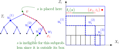
Figure 5: The query in the picture has three possible defining nodes $u_{i}^{(1)}$, $u_{i}^{(2)}$ and $u_{i}^{(3)}$ for its subproblems in $T_{i}$. $s$ will be ineligible for any subproblem that involves $u_{i}^{(3)}$ as its defining node.

Consider a query $\mbox{Dom}_{v_{1},\ldots,v_{d-1}}(q)$ and a sum $s$ that can be used to answer this query. By Observation 1, $s$ is stored at the subtree of a node $v_{i}$ in $T_{i}$ for every $1\leq i\leq d-1$ (see Figure 5 for an example). Consider the point $(x_{i},z_{i})$ that is used to define the query. We know the following: $v_{i}$ is the unique node in $T_{i}$ such that $\gamma(v_{i})$ contains $(x_{i},z_{i})$. Let $w_{i}$ be the leaf node in $T_{i}$ such that $r(w_{i})$ contains the point $q$ and let $\pi_{i}$ be the path that connects $v_{i}$ to $w_{i}$ (shown in red in Figure 5). Any node $u$ in $T_{i}$ that hangs to the left of the path $\pi$ could be a defining node of a subproblem of the query. In other words, if $u_{i}$ is a node $T_{i}$ that has a right sibling on $\pi_{i}$, then $u_{i}$ could be among the defining nodes of some subproblem of the query. Let $u^{(1)}_{i},\cdots,u^{(f_{i})}_{i}$ be the list of nodes with this property and let $\ell_{i}+j^{(k)}_{i}$ be the depth of $u^{(k)}_{i}$. Observe that the Cartesian product $\left\{u^{(1)}_{1},\cdots,u^{(f_{1})}_{1}\right\}\times\cdots\times\left\{u^{(1)}_{d-1},\cdots,u^{(f_{d-1})}_{d-1}\right\}$ captures all the possible tuples of $d-1$ nodes, one from each $T_{i}$, that are defining nodes of some subproblem of the query; every choice in this Cartesian product will yield a subproblem and for every subproblem its tuple of $d-1$ defining nodes can be found in this Cartesian product. Thus, for every ${\rm AJ}\in\left\{j^{(1)}_{1},\cdots,j^{(f_{1})}_{1}\right\}\times\cdots\times\left\{j^{(1)}_{d-1},\cdots,j^{(f_{d-1})}_{d-1}\right\}$ we have a ${\rm AJ}$-subproblem of the query with the corresponding defining nodes from the aforementioned Cartesian product.

Now let us look back at the sum $s$. The line segment $t_{i}(s)$ denotes the $X_{i}$-range of the sum $s$. Let us examine its projection on the $X_{i}Z_{i}$ plane and in the representative diagram $\Gamma_{i}$. The $X_{i}$-range of $t_{i}(s)$ could be disjoint from the $X_{i}$-range of some prefix of the list of nodes $u^{(1)}_{i},\cdots,u^{(f_{i})}_{i}$ as well as some suffices of this list. This means, there will be indices $f_{i}(s)$ and $e_{i}(s)$ such that $s$ cannot be used for any subproblem involving nodes $u^{(1)}_{i},\cdots,u^{(f_{i}(s)-1)}$ or the nodes $u^{(e_{i}(s)+1)}_{i},\cdots,u^{(f_{i})}$. However, for any subproblem ${\rm AJ}\in\mathscr{J}_{s}=\left\{j^{(f_{1}(s))}_{1},\cdots,j^{(e_{1}(s))}_{1}\right\}\times\cdots\times\left\{j^{(f_{d-1})}(s)_{d-1},\cdots,j^{(e_{d-1}(s))}_{d-1}\right\}$ $s$ can potentially be used for ${\rm AJ}$-subproblem, provided its $Y$-coordinate is below that of the query. We now estimate the volume of the intersection of $e(s)$ with $\mbox{Top}({\rm AJ},\lambda_{\rm AJ})$ for different ${\rm AJ}\in\mathscr{J}_{s}$.

Observe that $e(s)$ and $\mbox{Top}({\rm AJ},\lambda_{\rm AJ})$ will fully intersect along any dimension other than $Y$ for any ${\rm AJ}\in\mathscr{J}_{s}$. In fact, this property is the entire reason why we had to deal with extensions of sums rather than the sums themselves. However, observe that the $e(s)$ does not have a bottom boundary (or a lower bound) along the $Y$-axis and its top boundary is fixed. On the other hand, the top boundary of all boxes $\mbox{Top}({\rm AJ},\lambda_{\rm AJ})$ is $y$ but their bottom boundary is variable; it is $y-\beta_{\rm AJ}$ for a parameter $\beta_{\rm AJ}$ that depends on the subproblem. Consider two subproblems, ${\rm AJ}=(j_{1},\cdots,j_{d-1})$ and ${\rm AJ}^{\prime}=(j_{1}+x_{1},\cdots,j_{d-1}+x_{d-1})$ where $x_{i}\geq 0$. Remember that $\beta_{\rm AJ}$ was defined $\beta_{\rm AJ}=\Theta(\frac{\lambda_{\rm AJ}}{n}\prod_{i=1}^{d-1}2^{\ell_{i}+j_{i}})$. We now calculate the ratio $\beta_{{\rm AJ}^{\prime}}/\beta_{\rm AJ}$ and observe that

$$\frac{\beta_{{\rm AJ}^{\prime}}}{\beta_{\rm AJ}}=\Omega\left(\frac{\lambda_{{\rm AJ}^{\prime}}}{\lambda_{\rm AJ}}\right)\prod_{i=1}^{d-1}2^{x_{i}}=\Omega\left(\prod_{i=1}^{d-1}\frac{j_{i}2^{x_{i}}}{j_{i}+x_{i}}\right)=\Omega(\prod_{i=1}^{d-1}2^{x_{i}/2})$$

Let $y_{b}$ be the $Y$-coordinate of top boundary of $e(s)$. If $e(s)$ and $\mbox{Top}({\rm AJ},\lambda_{\rm AJ})$ intersect, it follows that $y-\beta_{\rm AJ}\leq y_{b}\leq y$. As discussed, $\beta_{{\rm AJ}^{\prime}}$ will be larger (by a $2^{x_{1}/2+\ldots+x_{d-1}/2}$ factor at least) which implies not only $e(s)$ and $\mbox{Top}({\rm AJ}^{\prime},\lambda_{{\rm AJ}^{\prime}})$ intersect, but the volume of their intersection is a factor $1-O(2^{-x_{1}/2-\ldots-x_{d-1}/2})$ fraction of the entire volume of $\mbox{Top}({\rm AJ}^{\prime},\lambda_{{\rm AJ}^{\prime}})$! As a result, this means that $e(s)$ will cover almost all the points of $\mbox{Top}({\rm AJ}^{\prime},\lambda_{{\rm AJ}^{\prime}})$ as long as $x_{1}+\cdots+x_{d-1}\geq c$ for a large enough constant $c$.

Fix a value $i$, $1\leq i\leq d-1$. Consider the $i$-th coordinate of all the subproblems $\mathscr{J}_{s}$. By what we have discussed, this coordinate can take any of the values in $\left\{j^{(f_{i}(s))}_{i},j^{(f_{i}(s)+1)}_{i},\cdots,j^{(e_{i}(s))}_{i}\right\}$. Consider a sum $s$ that can be used to answer a ${\rm AJ}$-subproblem for ${\rm AJ}=(j_{1},\cdots,j_{d-1})$. We consider two cases:

1. For all $i$, $1\leq i\leq d-1$, $j_{i}$ is among the $c$ largest values of the $i$-coordinate. It follows that there can be at most $c^{d-1}=O(1)$ such subproblems ${\rm AJ}$.

2. At least one value $j_{i}$ is not among the $c$ largest values of the $i$-coordinate, meaning, $j_{i}=j_{i}^{(k)}$ where $k<e_{i}(s)-c$. Consider value ${\rm AJ}^{\prime}=(j_{1},\cdots,j_{i-1},j_{i}^{(k+c)},j_{i+1},\cdots,j_{d-1})\in\mathscr{J}_{s}$ where we have only replaced the $i$-coordinate of ${\rm AJ}$ with a different value. And the value we have replaced it with has a rank $c$ higher. In this case, we know that $s$ almost entirely covers $\mbox{Top}({\rm AJ}^{\prime},\lambda_{{\rm AJ}^{\prime}})$. Now, we can charge any point that $s$ covers expensively in ${\rm AJ}$-subproblem to one point that $s$ covers cheaply in ${\rm AJ}^{\prime}$-subproblem. It is clear that any point in ${\rm AJ}^{\prime}$-subproblem can be charged at most $(d-1)$ times, since they can only be charged once along any dimension.

Now we are almost done. If a sum $s$ can cover points from many different subproblems, then it also covers a lot of points cheaply. However, we know that only a small fraction of the points in $\mbox{Top}(q)$ can be covered cheaply. As a result, at least a constant fraction of the points in $\mbox{Top}(q)$ should be covered by sums that are only used for a constant number of subproblems. Each such sum covers a constant number of points and thus the number of sums required to cover the points in $\mbox{Top}(q)$ is asymptotically bounded by Eq. 7. This concludes the proof.

4 The Upper Bounds

We build data structures for idempotent semigroups and for well-distributed point sets (or a set of $n$ points placed uniformly at random inside a square) and show that our analysis in the previous section is tight. Due to lack of space, the technical parts of the proof have been moved to the appendix but the main idea is to simulate the phenomenon we have captured in our lower bound: the idea that one can store sums such that the sums from different subproblems “help” each other. To do that, we define the notion of “collectively well-distributed” point sets. Intuitively, collectively well-distributed point sets is a collection of point sets $\mathscr{P}$ where each element of $\mathscr{P}$ is a well-distributed point set but importantly, certain unions of the point sets in $\mathscr{P}$ are also well-distributed point sets. See Fig. 6 for an example.

Figure 6: The point sets $P_{1},P_{2},P_{3},P_{4}$ are well-distributed. For any continuous set of integers $I\subset\left\{1,\dots,4\right\}$, $\cup_{i\in I}P_{i}$ is also well-distributed but $P_{1}\cup P_{3}$ might not be well-distributed.

Definition 4.1.

Let $\mathscr{I}=[t]^{k}$ be a set of indices, for an integer $t$ and a constant integer $k$. Let $\mathscr{P}$ be a collection of point sets of roughly equal size indexed by $I$. That is, for each $\mathrm{I}\in\mathscr{I}$, there exists a point set $P_{\mathrm{I}}\in\mathscr{P}$ containing $\Theta(n)$ points in $\mathbb{R}^{d}$. We say $\mathscr{P}$ is collectively well-distributed if the following holds for any $2k$ integers $1\leq i_{1}\leq j_{1}\leq t$, $1\leq i_{2}\leq j_{2}\leq t,\dots,$, and $1\leq i_{k}\leq j_{k}\leq t$: The point set $\cup_{i_{1}\leq\ell_{1}\leq j_{1}}\dots\cup_{i_{k}\leq\ell_{k}\leq j_{k}}P_{(\ell_{1},\dots,\ell_{k})}$ is well-distributed.

Lemma 5.

For every $N$, $h$, and given constants $d$, and $k$, there is a collectively well-distributed point set $\mathscr{P}$ indexed by $\mathscr{I}=[h]^{k}$ such that each point set in $\mathscr{P}$ contains $\Theta(N)$ points in $\mathbb{R}^{d}$.

Proof 4.2.

Our main idea is that we can obtain the collection $\mathscr{P}$ by projecting a well-distrusted point set in $\mathbb{R}^{d+k}$ down to $\mathbb{R}^{d}$. By Lemma 1, there exists a point set $\mathscr{P}$ of size $\Theta(Nh^{k})$ such that $\mathscr{P}$ is well-distributed in $\mathbb{R}^{d+k}$. Consider the dimensions $d+1,d+2,\dots,d+k$ of the $(d+k)$-dimensional unit cube $\mathcal{Q}$ and divide each side of $\mathcal{Q}$ along those dimensions into $t$ equal pieces. This divides $\mathcal{Q}$ into $h^{k}$ congruent subrectangles, and we naturally index them with elements of $[h]^{k}$, to obtain $h^{k}$ subrectangles $\mathcal{Q}_{\mathrm{I}}$, for $\mathrm{I}\in\mathscr{I}$. Let $P^{\prime}_{\mathrm{I}}$ be the subset of $\mathscr{P}$ in $\mathcal{Q}_{\mathrm{I}}$. By construction, the volume of $\mathcal{Q}_{\mathrm{I}}$ is $h^{-k}$, which by the properties of a well-distributed point set implies $|P^{\prime}_{\mathrm{I}}|=\Theta(N)$. Let $P_{\mathrm{I}}$ be the projection of $P^{\prime}_{\mathrm{I}}$ onto the first $d$-dimensions. We have $|P_{\mathrm{I}}|=\Theta(N)$.

Now consider $2k$ indices $1\leq i_{1}\leq j_{1}\leq h$, $1\leq i_{2}\leq j_{2}\leq h,\dots,$, and $1\leq i_{k}\leq j_{k}\leq h$ and the point set $X=\cup_{i_{1}\leq\ell_{1}\leq j_{1}}\dots\cup_{i_{k}\leq\ell_{k}\leq j_{k}}P_{(\ell_{1},\dots,\ell_{k})}$. Let $\mathscr{L}=\left\{(\ell_{1},\dots,\ell_{k})|i_{1}\leq\ell_{1}\leq j_{1},\dots,i_{k}\leq\ell_{k}\leq j_{k}\right\}$ which means $X=\cup_{\mathrm{I}\in\mathscr{L}}P_{\mathrm{I}}$. Define $\mathcal{Q}_{\mathscr{L}}=\cup_{\mathrm{I}\in\mathscr{L}}\mathcal{Q}_{\mathrm{I}}$. We now need to show that $X$ is well-distributed in $\mathbb{R}^{d}$. We show the property (iii) of a well-distributed point set, the other property follows very similarly. Consider a $d$-dimensional rectangle $r$ with ($d$-dimensional) volume $v$ inside the unit cube in $\mathbb{R}^{d}$. Let $r^{\prime}$ be the $(d+k)$-dimensional rectangle whose projection onto the first $d$ dimensions is $r$ and whose $(d+\ell)$-th side is the same as the $(d+\ell)$-th side of $\mathcal{Q}_{\mathscr{L}}$. Thus, the length of the $(d+\ell)$-th side of $\mathcal{Q}_{\mathscr{L}}$ is $\frac{j_{\ell}-i_{\ell}}{h}$ which implies the ($(d+k)$-dimensional) volume of $r^{\prime}$ is $v\frac{j_{1}-i_{1}}{h}\frac{j_{2}-i_{2}}{h}\dots\frac{j_{k}-i_{k}}{h}$. This implies $r^{\prime}$ contains $\Theta((v\prod_{\ell=1}^{k}\frac{j_{\ell}-i_{\ell}}{h}\cdot N)$ points but observe that $|X|=N\prod_{\ell=1}^{k}\Theta((j_{\ell}-i_{\ell}))$ which implies $r^{\prime}$ contains $\Theta(v|X|)$ points.

A rough sketch.

We first describe a rough sketch of our approach. Assume the input $P$ is a well-distributed point set and that we are interested in answering queries of the form $q=[a_{1},b_{1}]\times\dots\times[a_{k},b_{k}]\times(-\infty,b_{k+1}]\dots\times(-\infty,b_{d}]$. Let $h=\log n$. We use Lemma 5 to create a collection $\mathscr{D}$ containing $h^{k}$ point sets, with each point set containing $\Theta(n/\log^{k}n)$ points. These point sets are indexed by $\mathscr{I}=[h]^{k}$. Then, a point $X=(x_{1},\dots,x_{d})$ in the set $D_{\mathrm{I}}\in\mathscr{D}$ for $\mathrm{I}=(i_{1},\dots,i_{k})$ is turned into a $(d+k)$-sided box $B(X)$ in the form of $[\ell_{1},x_{1}]\times\dots\times[\ell_{k},x_{k}]\times(-\infty,x_{k+1}]\times\dots\times(-\infty,x_{d}]$. The index $i_{j}$, $1\leq j\leq k$ determines how long is the $j$-th side of the box $B(X)$, i.e., the length of the interval $[\ell_{j},x_{j}]$. This length will be around $1/2^{i_{j}}$. Next, we will analyse how to answer a query $q$. We will show this query can be reduced to answering up to $h^{k}$ different subproblems using a range tree approach, e.g., answering queries $q_{j_{1},j_{2},\dots,j_{k}}$ for (possibly) all choices of $j_{1},\dots,j_{k}\in[h]$. These subproblems will correspond to covering smaller and smaller regions. Crucially, since $\mathscr{D}$ was collectively well-distributed, it follows that the subproblems become progressively easier to answer. After some careful analysis, we will show that answering $q_{j_{1},j_{2},\dots,j_{k}}$ requires $\frac{h^{k}\log^{d-k}n}{\prod_{i=1}^{k}j_{i}}$ sums, asymptotically. Finally, we observe that the summing this bound over all choices of $j_{1},\dots,j_{k}\in[h]$ yields the desired bound and thus we prove the following theorem.

We now return to our main result of the section.

Theorem 4.3.

For a set $P$ of $n$ points placed uniformly randomly inside the unit cube in $\mathbb{R}^{d}$, one can build a data structure that uses $O(n)$ storage such that a $(d+k)$-sided query can be answered with the expected query bound of $O(\log^{d-1}n(\log\log n)^{k})$, for $1\leq k\leq d-1$.

If $P$ is well-distributed, then the query bound can be made worst-case.

We now present the details.

Chazelle [8] showed that for a set of randomly placed points inside the unit cube, one can build an efficient data structure matching his lower bound. The same analysis can be applied to a well-distributed point set to obtain a worst-case query bound; after all, a well-distributed point set guarantees that a shape of volume $v$ contains $\Theta(nv)$ points whereas a randomly placed point set only guarantees it in the expectation. Furthermore, the analysis can be easily generalized to obtain a trade-off curve for when less than $n$ storage is used by the data structure. Thus, we can have the following result.

Lemma 6.

[8] Let $n$ and $m$ be parameters such that $1<m<n/2$ and let $S$ be a well-distributed points in $\mathcal{Q}$ containing $n/m$ points. Consider an input point set $P$ containing $n$ points. We can build a data structure $D$ by summing the weights of all the points of $P$ dominated by a point $s\in S$. $D$ will use at most $m$ storage and it can answer any dominance query $q$ with the expected query bound of $O(m\log^{d-1}n)$ if $P$ is uniformly randomly placed in $\mathcal{Q}$. If $P$ is a well-distributed point set, then the query bound is worst-case.

Proof 4.4 (Proof summary.).

Let $t=n/m$. Consider a query $q$ and let $X\subset S$ be the set of points dominated by $q$. Let $M$ be the maxima of $X$, i.e., subset of $X$ that are not dominated by points in $X$. Chazelle has shown that $|M|=O(\log^{d-1}t)=O(\log^{d-1}n)$ and that the volume of the region $R$ that is dominated by $q$ but not by any point in $M$ is $O(\frac{\log^{d-1}n}{t})=O(m\log^{d-1}n/n)$. So, $R$ will on average contain $O(m\log^{d-1}n)$ points of $P$. To answer $q$, we cover the points in $R$ with singletons and the remaining points using the points in $M$. If $P$ is well-distributed, $R$ will contain $O(m\log^{d-1}n)$ points in the worst-case since it can be decomposed into $O(|M|)$ rectangles.

We also need the following definition and lemma.

Definition 4.5.

Let $T$ be a balanced binary tree with height $h$, built on the interval $[z_{1},z_{2}]\subset[0,1]$ and by repeatedly partitioning it in half. In particular, every node $u\in T$ is assigned an interval $[a(u),b(u)]\subset[z_{1},z_{2}]$, the root is assigned the interval $[z_{1},z_{2}]$, the left child of $v$ is assigned the interval $[a(u),\frac{a(u)+b(u)}{2}]$ and the right child of $v$ is assigned the interval $[\frac{a(u)+b(u)}{2},b(u)]$. Two nodes $u$ and $w$ in $T$ are said to be adjacent if they are at the same depth and $a(u)=b(w)$ or $b(u)=a(w)$; if $b(u)=a(w)$ then we say $u$ it the left neighbor of $w$. A balanced prefix cover of a leaf $v$ is defined as follows: it is a sequence of $h^{\prime}\leq 2h$ pairs of nodes $(u_{1},w_{1}),\dots,(u_{h^{\prime}},w_{h^{\prime}})$ such that $u_{i}$ is the left neighbor of $w_{i}$ and the interval $[z_{1},a(v)]$ is the disjoint union of the intervals $[a(u_{1}),b(u_{1})],[a(u_{2}),b(u_{2})],\dots,[a(u_{h^{\prime}}),b(u_{h^{\prime}})]$. Furthermore, no three nodes $u_{i},u_{k},u_{j}$ can have the same depth. See Figure 7.

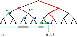
Figure 7: A balanced prefix cover. A pair $(u_{i},w_{i})$ is shown with a blue arrow from $w_{i}$ to $u_{i}$. The intervals $[a(u_{1}),b(u_{1})],\dots,[a(u_{h^{\prime}}),b(u_{h^{\prime}})]$, shown with alternating colors, disjointly cover $[z_{1},a(v)]$.

Lemma 4.6.

Let $T$ be a balanced binary tree with height $h$. For any leaf $u$, there exists a balanced prefix cover of $u$.

Proof 4.7.

Let $\pi$ be the path that connects the root of $T$ to $u$ and let $x_{1},\dots,x_{k}$ be the nodes that hang to the left of $\pi$, ordered from left to right. Observe that the depth of the nodes $x_{1},\dots,x_{k}$ is strictly increasing. To obtain the balanced prefix cover, we use the following procedure. We initialize a sequence of nodes, called the active sequence, with the list $x_{1},\dots,x_{k}$ (the red nodes in Fig 7). Then, we perform the following until the active sequence contains only one node. Consider the first two elements of the active sequence, $x_{1}$ and $x_{2}$. (i) If they have the same depth, then we create the pair $(x_{1},x_{2})$ and then remove $x_{1}$ but (ii) otherwise, we replace $x_{1}$ with $x_{\ell}$ and $x_{r}$ where $x_{\ell}$ and $x_{r}$ are its left and right children.

These operations maintain that the depth of the nodes in the active sequence is always strictly increasing, except possibly for the first two nodes in the sequence. Furthermore, if the depth of $x_{1}$ is smaller than the depth of $x_{2}$, then first we perform operation (i) and then immediately perform operation (ii). The net effect is that the depth of the first element is increased by one. This might cause for the depth of the first element to be equal to the depth of the second element but then in the next iteration, operation (i) will remove the first element. Thus, in overall, the operations create at most two pairs for every depth, thus, the number of pairs is at most $2h$.

Our main result of the section is the following. See 4.3 Let $\mathcal{Q}$ be the unit cube in $\mathbb{R}^{d}$. Assume, the queries we would like to answer are in the form of $q=[a_{1},b_{1}]\times\dots\times[a_{k},b_{k}]\times(-\infty,b_{k+1}]\dots\times(-\infty,b_{d}]$. We build a balanced binary tree for each of the first $k$ dimensions, of height $h=\log n$. Let $T_{1},\dots,T_{k}$ be these binary trees, where $T_{i}$ is built on the $i$-th dimension and on the $i$-th side of the cube $\mathcal{Q}$ (the interval $[0,1]$). The nodes at depth $j$ of tree $T_{i}$ decompose $\mathcal{Q}$ into $2^{j}$ congruent “slabs” using hyperplanes that are perpendicular to the $i$-th axis. The slab of a node $v\in T_{i}$ is denoted by $r(v)$; this slab is defined by two hyperplanes perpendicular to the $i$-th axis at points $a(v)$ and $b(v)$. Let $m(v)=\frac{a(v)+b(v)}{2}$.

Before describing the data structure, we briefly look to see what entails to answer the query $q$. Consider the $i$-th dimension of the query for $1\leq i\leq k$ and the tree $T_{i}$. Consider the highest node $v\in T_{i}$ such that $m(v)$ lies inside the interval $[a_{i},b_{i}]$. We can now partition the interval $[a_{i},b_{i}]$ into two intervals $[a_{i},m(v)]$ and $[m(v),b_{i}]$ which in turn partitions $q$ into two queries, and over all indices $i$, this partitions $q$ into $2^{k}$ queries. In the remainder of the proof, we will focus on how to answer the query that corresponds to $[m(v),b_{i}]$, for $1\leq i\leq k$, as the other queries can be handled in a similar fashion.

We now describe the data structure. We use Lemma 5 with $h=\log n$, $N=n/h^{k}$ to obtain the collection of sets $\mathscr{D}$ containing $h^{k}$ point sets indexed by the index set $\mathscr{I}=[h]^{k}$. Using, the binary trees $T_{1},\dots,T_{k}$, we turn each point in the collection of points $\mathscr{D}$ into a $(d+k)$-dimensional region which is then the data structure stores (i.e., the data structure stores the sum of the weights of the points inside the region). This is done in the following way. Consider a point $X\in D_{\mathrm{I}}$ for $D_{\mathrm{I}}\in\mathscr{D}$ and assume $I=(i_{1},\dots,i_{k})\in[h]^{k}$ and $X=(x_{1},\dots,x_{d})\in\mathbb{R}^{d}$. We turn the point $X$ into the range $B(X)=[\ell_{1},x_{1}]\times[\ell_{2},x_{2}],\dots,[\ell_{k},x_{k}]\times(-\infty,x_{k+1}]\times\dots\times(-\infty,x_{d}]$ where the coordinate $\ell_{j}$, $1\leq j\leq k$, is obtained as follows: we look at $T_{j}$ and find a node $u\in T_{j}$ at depth $i_{j}$ such that $r(u)$ contains $X$; then we consider the left neighbor $v$ of $u$ and we set $\ell_{j}$ to $a(v)$. In some exceptional cases $v$ might not exist, in particular, when $X$ is inside $r(u)$ and $u$ is the leftmost node at depth $i_{j}$; in such cases $B(X)$ is not defined. It is clear that the data structure stores $O(n)$ sums, since the total number of points contained in the point set of $\mathscr{D}$ is $O(n)$.

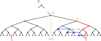
Figure 8: Answering a query.

Now, consider a query range $q=[a_{1},b_{1}]\times\dots\times[a_{k},b_{k}]\times(-\infty,b_{k+1}]\dots\times(-\infty,b_{d}]$. Consider the interval $[a_{i},b_{i}]$ for $1\leq i\leq k$ and the tree $T_{i}$. Let $v^{\prime}_{i}$ be the highest node in $T_{i}$ such that $a_{i}\leq m(v^{\prime}_{i})\leq b_{i}$. As previously alluded, we can decompose the query into two queries at node $v^{\prime}_{i}$: let $v_{i}$ be the right child of $v^{\prime}_{i}$ and $u_{i}$ be the leaf of $T_{i}$ such that $r(u_{i})$ contains the point $(b_{1},\dots,b_{d})$. We now consider the tree $T_{i}(v_{i})$, i.e., the tree that hangs off at the node $v_{i}$. By Lemma 4.6, we can find a balanced prefix cover as a sequence of pairs $(u_{i,j},w_{i,j})$, $1\leq j\leq h^{\prime}_{i}$ that cover the interval $[m(v^{\prime}_{i}),a(u_{i})]$. See Figure 8. Thus,

$$[m(v^{\prime}_{i}),b_{i}]=[a(u_{i}),b_{i}]\cup\bigcup_{j=1}^{h^{\prime}_{i}}[a(u_{i,j}),b(u_{i,j})].$$ (10)

By construction, the region $[a_{1},b_{1}]\times\dots[a_{i-1},b_{i-1}]\times[a(u_{i}),b_{i}]\times\ldots\times[a_{k},b_{k}]\times(-\infty,b_{k+1}]\dots\times(-\infty,b_{d}]$ (where the $i$-th side of $q$ is replaced by the interval $[a(u_{i}),b_{i}]$) has volume at most $1/n$ and thus contains $O(1)$ input points on average; they can be covered by singletons (or in case of a well-distributed input, $O(1)$ singletons in the worst-case). To cover the rest of the query, we observe that region we would like to cover is the Cartesian product of a series of intervals given by Eq. 10 over all indices $1\leq i\leq k$. Thus, we need to cover the regions

$$q_{j_{1},j_{2},\dots,j_{k}}=[a(u_{1,j_{1}}),b(u_{1,j_{1}})]\times\dots\times[a(u_{k,j_{k}}),b(u_{k,j_{k}})]\times(-\infty,b_{k+1}]\dots\times(-\infty,b_{d}]$$ (11)

for all choices of $1\leq j_{1}\leq h^{\prime}_{1}$, and $1\leq j_{2}\leq h^{\prime}_{2}$, and so on until $1\leq j_{k}\leq h^{\prime}_{k}$.

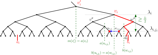
Figure 9: Answering a query.

Lemma 4.8.

Consider a fixed query $q_{j_{1},j_{2},\dots,j_{k}}$ obtained from query $q^{\prime}$ as outlined above. Consider a set $D_{\mathrm{I}}$ such that $\mathrm{I}=(z_{2},\dots,z_{k})$, $\lambda_{i}\leq z_{i}\leq\lambda_{i,j_{i}}$ for $1\leq i\leq k$. Consider a point $X\in D_{\mathrm{I}}$ such that $X\in\cap_{i=1}^{k}r(w_{i,j_{i}})$. We claim the following: (i) $i$-th dimension, $[\ell_{i},x_{i}]$, of the box $B(X)$ fits inside the $i$-th dimension of the query $q^{\prime}$, $[a(v_{i}),b_{i}]$. (ii) for any input point $p=(p_{1},\dots,p_{d})\in q_{j_{1},j_{2},\dots,j_{k}}$, the $i$-th coordinate, $p_{i}$, of $p$ for $1\leq i\leq k$ is within the $i$-th side of $B(X)$.

Proof 4.9.

Our first observation is the following: the node $u_{i,j_{i}}$ has at least $j_{i}/2$ ancestors between itself and the node $v_{i}$. That is, if $\lambda_{i}$ is the depth of $v_{i}$ and $\lambda_{i,j_{i}}$ is the depth of $u_{i,j_{i}}$, we have $\lambda_{i,j_{i}}-\lambda_{i}\geq j_{i}/2$. This observation follows because a balanced prefix cover contains at most two pairs in a given depth of a tree. Since $X\in\cap_{i=1}^{k}r(w_{i,j_{i}})$, it follows that $x_{i}\leq b(w_{i,j_{i}})\leq b_{i}$ and furthermore, since $\lambda_{i}\leq z_{i}\leq\lambda_{i,j_{i}}$, $\ell_{i}$ is set to $a(v^{\prime\prime}_{i})$ for some node $v^{\prime\prime}_{i}$ that is a descendant of $v^{\prime}_{i}$, which implies $a(v_{i})\leq a(v^{\prime\prime}_{i})=\ell_{i}$. This proves claim (i).

We now consider claim (ii). Observe that $p_{i}$ is between $a(u_{i,j_{i}})$ and $b(u_{i,j_{i}})$ and thus $p_{i}\in[a(u_{i,j_{i}}),b(u_{i,j_{i}})]$; however, $\ell_{i}$ is set to $a(v^{\prime\prime})$ for a node $v^{\prime\prime}$; also $v^{\prime\prime}$’s right neighbor, $w^{\prime\prime}$, is such that $r(w^{\prime\prime})$ contains $X$. We have two cases: in case (i), $w^{\prime\prime}$ is also the ancestor of $u_{i,j_{i}}$. In this case $\ell_{i}$ is set to the same value as $a(u_{i,j_{i}})$ and thus the $i$-th side of the box $B(X)$ is the interval $[a(u_{i,j_{i}}),x_{i}]$ but since $x_{i}>b(u_{i,j_{i}})$ this interval contains the interval $[a(u_{i,j_{i}}),b(u_{i,j_{i}})]$. In the second case, the ancestor of $u_{i,j_{i}}$ at depth $j_{i}$ is a node $v^{\prime\prime}$ that is the left neighbor of $w^{\prime\prime}$. In this case, $\ell_{i}$ is set to $a(v^{\prime\prime})$ and thus it is smaller than $a(u_{i,j_{i}})$ and thus once again the interval $[a(u_{i,j_{i}}),b(u_{i,j_{i}})]$ is contained in the $i$-th side of the box $B(X)$.

Let $\mathscr{I}^{\prime}$ be the set of indices $\mathrm{I}$ such that $\mathrm{I}=(z_{1},\dots,z_{k})$, $\lambda_{i}\leq z_{i}\leq\lambda_{i,j_{i}}$ for $1\leq i\leq k$. Note that the previous lemma (Lemma 4.8) holds for any point $X\in D_{\mathrm{I}}$ and for any $\mathrm{I}\in\mathscr{I}^{\prime}$. Observe that $|\mathscr{I}^{\prime}|\geq\frac{j_{1}j_{2}\dots j_{k}}{2^{k}}$ since $\lambda_{i,j_{i}}-\lambda_{i}\geq j_{i}/2$. Let $\mathscr{X}=\cup_{\mathrm{I}\in\mathscr{I}^{\prime}}D_{\mathrm{I}}$. As every set in $\mathscr{D}$ has asymptotically the same number of points, we have

$$|\mathscr{X}|=\Omega\left(\frac{n\prod_{i=1}^{k}j_{i}}{h^{k}}\right).$$

Consider two rectangles $R_{1}=\cap_{i=1}^{k}r(w_{i,j_{i}})$, and $R_{2}=\cap_{i=1}^{k}r(u_{i,j_{i}})$. Observe that they have the same $d$-dimensional volume since $u_{i,j_{i}}$ and $w_{i,j_{i}}$ have equal depth. Let $\alpha$ be this volume. Also observe that $q_{j_{1},j_{2},\dots,j_{k}}$ is inside $R_{2}$. Let $\mathscr{X}^{\prime}$ be the subset of $\mathscr{X}$ that lies inside $R_{1}$. By Lemma 4.8, for every point $X\in\mathscr{X}^{\prime}$ the box $B(X)$ stored by the data structure covers the $i$-th dimension of every input point $p\in q_{j_{1},j_{2},\dots,j_{k}}$ for $1\leq i\leq k$. So in essence, we only need to take care of the last $d-k$ dimensions. We do that by projection onto the last $d-k$ dimensions: Let $P^{\prime}$, $q^{\prime}$ and $\mathscr{X}^{\prime\prime}$ be the projection of the subset of input points that lie inside $R_{1}$, $q_{j_{1},j_{2},\dots,j_{k}}$, and $\mathscr{X}^{\prime}$ onto the last $d-k$ dimensions, respectively. Based on what we discussed, the problem has been reduced to answering the $(d-k)$-dimensional dominance query $q^{\prime}$ on the point set $P^{\prime}$ using sums stored in $\mathscr{X}^{\prime\prime}$; each such sum is the sum of the weights in a dominance region. Now, we use Lemma 6.

Since the set of input points $P$ is well-distributed, it follows that $P^{\prime}$ contains $O(n\alpha)$ points. Since the collection $\mathscr{D}$ is collectively well-distributed, it follows that $\mathscr{X}^{\prime\prime}$ contains $\Omega(|\mathscr{X}|\alpha)$ points. Thus, by Lemma 6, the $(d-k)$-dimensional query $q^{\prime}$ on a set of $n^{\prime}=|P^{\prime}|$ points, using storage $\Omega(|\mathscr{X}|\alpha)=\Omega\left(\frac{n\alpha\prod_{i=1}^{k}j_{i}}{h^{k}}\right)$, can be answered with asymptotic query bound of

$$\frac{h^{k}\log^{d-k}n}{\prod_{i=1}^{k}j_{i}}.$$ (12)

Note that the Eq. 12 is only for a fixed query $q_{j_{1},j_{2},\dots,j_{k}}$. Thus, the total query bound is sum of the bound offered by Eq. 12 over all possible choice of indices $j_{1},\dots,j_{k}$:

$$\sum_{j_{1}=1}^{h^{\prime}_{1}}\sum_{j_{2}=1}^{h^{\prime}_{2}}\dots\sum_{j_{k}=1}^{h^{\prime}_{k}}\frac{h^{k}\log^{d-k}n}{\prod_{i=1}^{k}j_{i}}=\log^{d}n\cdot O\left(\sum_{j_{1}=1}^{h^{\prime}_{1}}\sum_{j_{2}=1}^{h^{\prime}_{2}}\dots\sum_{j_{k-1}=1}^{h^{\prime}_{k-1}}\frac{\log\log n}{\prod_{i=1}^{k-1}j_{i}}\right)=O(\log^{d}n(\log\log n)^{k}).$$

For a randomly placed point set, Lemma 6 offers an expected query bound and thus we obtain the expected query bound of $O(\log^{d-1}n(\log\log n)^{k})$. However, if the input point set is well-distributed, we get the same bound but in the worst-case.

5 Conclusions

In this paper we considered the semigroup range searching problem from a lower bound point of view. We improved the best previous lower bound trade-off offered by Chazelle by analysing a well-distributed point set for $(2d-1)$-sided queries for an idempotent semigroup. Furthermore, we showed that our analysis is tight which leads us to suspect that we have found an (almost) optimal lower bound for idempotent semigroups as we believe it is unlikely that a more difficult point set exists. Thus, two prominent open problems emerge: (i) Can we improve the known data structures under the extra assumption that the semigroup is idempotent? (ii) Can we improve our lower bound under the extra assumption that the semigroup is not idempotent? Note that the effect of idempotence on other variants of range searching was studied at least once before [5].

References

- [1] Peyman Afshani, Lars Arge, and Kasper Green Larsen. Higher-dimensional orthogonal range reporting and rectangle stabbing in the pointer machine model. In Symposium on Computational Geometry (SoCG), pages 323–332, 2012. doi:http://doi.acm.org/10.1145/2261250.2261299.
- [2] Peyman Afshani and Anne Drimel. On the complexity of range searching among curves. In Proceedings of the Annual ACM-SIAM Symposium on Discrete Algorithms (SODA), pages 898–917, 2017.
- [3] Pankaj K. Agarwal. Range searching. In J. E. Goodman, J. O’Rourke, and C. Toth, editors, Handbook of Discrete and Computational Geometry. CRC Press, Inc., 2016.
- [4] N. Alon and B. Schieber. Optimal preprocessing for answering on-line product queries. Technical Report 71/87, Tel-Aviv University, 1987.
- [5] Sunil Arya, Theocharis Malamatos, and David M. Mount. On the importance of idempotence. In Proceedings of ACM Symposium on Theory of Computing (STOC), pages 564–573, 2006.
- [6] Jon Louis Bentley. Decomposable searching problems. Information Processing Letters (IPL), 8(5):244 – 251, 1979.
- [7] Jon Louis Bentley. Multidimensional divide-and-conquer. Communications of the ACM (CACM), 23(4):214–229, 1980.
- [8] Bernard Chazelle. Lower bounds for orthogonal range searching: part II. the arithmetic model. Journal of the ACM (JACM), 37(3):439–463, 1990.
- [9] Michael L. Fredman. The inherent complexity of dynamic data structures which accommodate range queries. In Proc. 21stProceedings of Annual IEEE Symposium on Foundations of Computer Science (FOCS), pages 191–199, October 1980.
- [10] Michael L. Fredman. A lower bound on the complexity of orthogonal range queries. Journal of the ACM (JACM), 28(4):696–705, 1981.
- [11] Michael L. Fredman. Lower bounds on the complexity of some optimal data structures. SIAM Journal of Computing, 10(1):1–10, 1981.
- [12] Robert Endre Tarjan. A class of algorithms which require nonlinear time to maintain disjoint sets. Journal of Computer and System Sciences (JCSS), 18(2):110 – 127, 1979.
- [13] Andrew C. Yao. Space-time tradeoff for answering range queries (extended abstract). In Proceedings of ACM Symposium on Theory of Computing (STOC), STOC ’82, pages 128–136. ACM, 1982.