Toward a First-Principles Calculation of Electroweak Box Diagrams

Abstract

We derive a Feynman-Hellmann theorem relating the second-order nucleon energy shift resulting from the introduction of periodic source terms of electromagnetic and isovector axial currents to the parity-odd nucleon structure function $F_{3}^{N}$. It is a crucial ingredient in the theoretical study of the $\gamma W$ and $\gamma Z$ box diagrams that are known to suffer from large hadronic uncertainties. We demonstrate that for a given $Q^{2}$, one only needs to compute a small number of energy shifts in order to obtain the required inputs for the box diagrams. Future lattice calculations based on this approach may shed new light on various topics in precision physics including the refined determination of the Cabibbo-Kobayashi-Maskawa matrix elements and the weak mixing angle.

The electroweak box diagrams involving the exchange of a photon and a heavy gauge boson ($W^{\pm}/Z$) between a lepton and a hadron (see Fig. 1) represent an important component in the standard model (SM) electroweak radiative corrections that enter various low-energy processes such as semileptonic decays of hadrons and parity-violating lepton-hadron scatterings. These are powerful tools in extractions of SM weak parameters. The precise calculations of such diagrams are, however, extremely difficult because they are sensitive to the loop momentum $q$ at all scales and include contributions from all possible virtual hadronic intermediate states which properties are governed by quantum chromodynamics (QCD) in its nonperturbative regime. Hence, they are one of the main sources of theoretical uncertainty in the extracted weak parameters such as the Cabibbo-Kobayashi-Maskawa (CKM) matrix elements Hardy and Towner (2015, 2018) and the weak mixing angle Kumar et al. (2013) at low scale.

Modern treatments of the box diagrams are based on the pioneering work by Sirlin Sirlin (1978) in the late 1970s that separates the diagrams into “model-independent” and “model-dependent” terms, of which the former can be reduced to known quantities by means of current algebra. The model-dependent terms, on the other hand, consist of the interference between the electromagnetic and the axial weak currents, and are plagued with large hadronic uncertainties at $Q^{2}\lesssim 1$ GeV². Earlier attempts to constrain these terms include varying the infrared cutoff Marciano and Sirlin (1983, 1984, 1986); Bardin et al. (2001) and the use of interpolating functions Marciano and Sirlin (2006), but all these methods suffer from nonimprovable theoretical uncertainties. The recent introduction of dispersion relations in treatments of the $\gamma Z$ Gorchtein and Horowitz (2009); Gorchtein et al. (2011); Blunden et al. (2011); Rislow and Carlson (2013) and $\gamma W$ Seng et al. (2018a, b); Gorchtein (2018) boxes provides a better starting point to the problem by expressing the loop integral in terms of parity-odd structure functions. Since the latter depend on on-shell intermediate hadronic states, one could in principle relate them to experimental data. Unfortunately, at the hadronic scale such data either do not exist or belong to a separate isospin channel which can only be related to our desired structure functions within a model.

First-principles calculations of the parity-odd structure functions from lattice QCD have not yet been thoroughly investigated, and are expected to be challenging due to the existence of multihadron final states. Moreover, most of the recent developments in the lattice calculation of parton distribution functions (see, e.g. Ref. Lin et al. (2018)) do not apply here because their applicability is restricted to large $Q^{2}$. But at the same time we also observe an encouraging development in the application of the Feynman-Hellmann theorem (FHT) Feynman:1939zza ; Hellmann , where external source terms are added to the Hamiltonian, and the required hadronic matrix elements of the source operator could be related to the energy shift of the corresponding hadron which is easier to obtain on lattice as it avoids the calculation of complicated (and potentially noisy) contraction diagrams. A nonzero momentum transfer $\vec{q}$ can also be introduced by adopting a periodic source term. Such a method shows great potential in the calculation of hadron electromagnetic form factors Chambers et al. (2017a), Compton scattering amplitude Agadjanov et al. (2017, 2019), parity-even nucleon structure functions Chambers et al. (2017b), and hadron resonances RuizdeElvira:2017aet . Furthermore, it does not involve any operator product expansion so its applicability is not restricted to large $Q^{2}$.

Based on the developments above, we propose in this Letter a new method to study the $\gamma W$/$\gamma Z$ boxes, namely to compute a generalized parity-odd forward Compton tensor on the lattice through the second-order nucleon energy shift upon introducing two periodic source terms, and solve for the moments of $F_{3}$ through a dispersion relation. We will demonstrate that for a given $Q^{2}$, the calculation of a few energy shifts already provides sufficient information about the integrand of the box diagrams, and such a calculation is completely executable with the computational power in the current lattice community. When data are accumulated for sufficiently many values of $Q^{2}$ at the hadronic scale, one will eventually be able to remove the hadronic uncertainties in the electroweak boxes and provide a satisfactory solution to this long-lasting problem in precision physics.

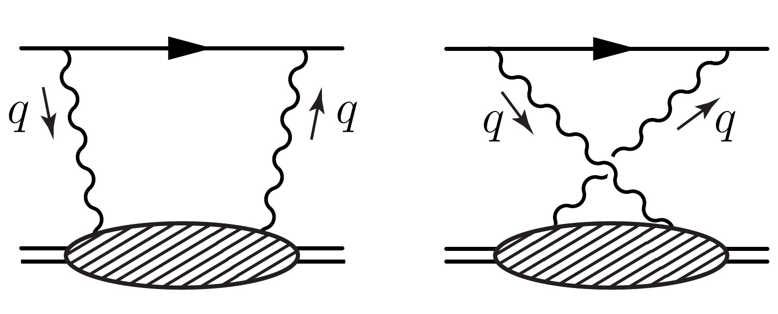
Figure 1: Direct and crossed box diagrams. Single and double lines represent a lepton and a hadron, respectively. The blob represents hadronic excitations and the wiggly lines denote the gauge bosons.

We start by defining the electromagnetic current and the isovector axial current (here we neglect the strange current just to simplify our discussions of the two examples below, but it is not a necessary approximation) :

$$J_{em}^{\mu} = (2/3)\bar{u}\gamma^{\mu}u-(1/3)\bar{d}\gamma^{\mu}d$$

$$J_{A}^{\mu} = \bar{u}\gamma^{\mu}\gamma_{5}u-\bar{d}\gamma^{\mu}\gamma_{5}d.$$ (1)

The spin-independent, parity-odd nucleon structure function $F_{3}^{N}$ ($N=p,n$) can be defined through the hadronic tensor:

$$W^{\mu\nu}_{N}(p,q) = \frac{1}{4\pi}\int d^{4}xe^{iq\cdot x}\left\langle N(\vec{p})\right|[J_{em}^{\mu}(x),J_{A}^{\nu}(0)]\left|N(\vec{p})\right\rangle$$ (2)

$$= -\frac{i\varepsilon^{\mu\nu\alpha\beta}q_{\alpha}p_{\beta}}{2p\cdot q}F_{3}^{N}(x_{B},Q^{2}),$$

where $x_{B}=Q^{2}/(2p\cdot q)$ is the Bjorken variable which lies between $-1$ and $1$, and $\varepsilon^{0123}=-1$. We stress that it is more natural to include negative values of $x_{B}$ because in a dispersion relation involving $F_{3}^{N}(x_{B},Q^{2})$, $x_{B}$ acts as the integration variable in the Cauchy integral that could lie on both the positive and the negative real axes. Notice that the spin label in the nucleon states are suppressed for simplicity. From that we may define the so-called “first Nachtmann moment” of $F_{3}^{N}$ as Nachtmann (1973, 1974)

$$M_{1}[F_{3}^{N}]=\int_{0}^{1}dx\Pi(x,Q^{2})F_{3}^{N}(x,Q^{2}),$$ (3)

where

$$\Pi(x,Q^{2})=\frac{4}{3}\frac{1+2\sqrt{1+4m_{N}^{2}x^{2}/Q^{2}}}{(1+\sqrt{1+4m_{N}^{2}x^{2}/Q^{2}})^{2}}$$ (4)

and $m_{N}$ is the nucleon mass.

To see the physical relevance of the definitions above, we shall briefly discuss some recent progress in the study of two weak processes that play central roles in low-energy precision tests of SM:

First, superallowed nuclear $\beta$ decays represent the best avenues for the measurement of the CKM matrix element $V_{ud}$ as the corresponding weak nuclear matrix element is protected at tree level by the conserved vector current. With the inclusion of higher-order corrections one obtains Hardy and Towner (2015):

$$|V_{ud}|^{2}=\frac{2984.432(3)\>\mathrm{s}}{\mathcal{F}t(1+\Delta_{R}^{V})}$$ (5)

where $\mathcal{F}t$ is the product between the half-life $t$ and the statistical function $f$, but modified by nuclear-dependent corrections. $\Delta_{R}^{V}$ represents the nucleus-independent radiative correction. The main theoretical uncertainty of $|V_{ud}|$ comes from $\Delta_{R}^{V}$, which in turn acquires its largest uncertainty from the interference between the isosinglet electromagnetic current and the axial charged weak current in the $\gamma W$ box diagram. The latter can be expressed as:

$$\left(\Delta_{R}^{V}\right)_{\gamma W}^{VA}=\int_{0}^{\infty}\frac{dQ^{2}}{Q^{2}}\frac{3\alpha}{\pi}\frac{M_{W}^{2}}{M_{W}^{2}+Q^{2}}M_{1}[F_{3}^{(0)}],$$ (6)

where $F_{3}^{(0)}=-(1/4)(F_{3}^{p}-F_{3}^{n})$ through isospin symmetry. A recent determination of $\Delta_{R}^{V}$ based on a dispersion relation and neutrino scattering data gives 0.02467(22) Seng et al. (2018a), which lies significantly above the previous sate-of-the-art result of 0.02361(38) Marciano and Sirlin (2006) and leads to an apparent violation of the first-row CKM unitarity at the level of 4$\sigma$ that calls for an immediate resolution. Besides, scrutinizing the problems in $V_{ud}$ will also lead to a better determination of $V_{us}$, because one of the main measuring channels of the latter, the $K\to\mu\nu(\gamma)$ decay, probes the ratio $|V_{us}|/|V_{ud}|$.

Second, we look at parity-odd $ep$ scattering. The measurement of the proton weak charge $Q_{W}^{p}$ in the almost-forward elastic $ep$ scattering is a powerful probe of the physics beyond SM due to the accidental suppression of its tree-level value $1-4\sin^{2}\theta_{W}$, with $\theta_{W}$ the weak mixing angle. After including one-loop electroweak radiative corrections, the quantity reads Erler et al. (2003)

$$Q_{W}^{p} = (1+\Delta\rho+\Delta_{e})[1-4\sin^{2}\theta_{W}(0)+\Delta_{e}^{\prime}]$$ (7)

$$+\Box_{WW}+\Box_{ZZ}+\Box_{\gamma Z},$$

among which $\Box_{\gamma Z}$ represents the contribution from the $\gamma Z$ box that bears the largest hadronic uncertainty. In the limit of vanishing beam energy, it takes the following form:

$$\Box_{\gamma Z}=\int_{0}^{\infty}\frac{dQ^{2}}{Q^{2}}\frac{3\alpha}{2\pi}v_{e}\frac{M_{Z}^{2}}{M_{Z}^{2}+Q^{2}}M_{1}[F_{3}^{\gamma Z}],$$ (8)

where $v_{e}$ is the electron weak charge and $F_{3}^{\gamma Z}=-F_{3}^{p}$. A recent estimation of $\Box_{\gamma Z}$ reads $0.0044(4)$ Blunden et al. (2011). In view of the upcoming P2 experiment at the Mainz Energy-Recovering Superconducting Accelerator (MESA) that aims for the measurement of $\sin^{2}\theta_{W}$ to a precision of $0.15\%$ Becker et al. (2018), it is necessary for a revisit of the $\gamma Z$ box to proceed coherently with $\gamma W$ in order to ensure there is no unaccounted systematics as recently discovered in the latter Seng et al. (2018a, b).

From the two examples above one sees that the object of interest is the first Nachtmann moment of $F_{3}^{N}$, which probes different on-shell intermediate states at different $Q^{2}$. The analysis of the data accumulated for an analogous parity-odd structure function $F_{3}^{WW}$ resulting from the interference between the vector and axial charged weak current in inclusive $\nu p/\bar{\nu}p$ scattering indicates that (1) at $Q^{2}<0.1$ GeV² the first Nachtmann moment is saturated by the contribution from the elastic intermediate state and the lowest nucleon resonances Bolognese et al. (1983) of which sufficient data are available, and (2) at $Q^{2}>2$ GeV² it is well described by a parton model with well-known perturbative QCD corrections Kataev and Sidorov (1994); Kim et al. (1998) (see also, Sec. IV of Ref. Seng et al. (2018b) for a detailed description of the dominant physics that takes place at different $Q^{2}$). On the other hand, multihadron intermediate states dominate at $Q^{2}\lesssim 1$ GeV², and a first-principles theoretical description at this region is absent so far. Although there are attempts to relate, say, $F_{3}^{(0)}$ to the measured $F_{3}^{WW}$ in this region, such a relation is only established within a model because it belongs to different isospin channels. Therefore, the goal of this Letter is to outline a method that allows for a reliable first-principles calculation of $M_{1}[F_{3}^{N}]$ at $Q^{2}\lesssim 1$ GeV².

To achieve this goal, we consider the following generalized forward Compton tensor:

$$T_{N}^{\mu\nu}(p,q) = \int d^{4}xe^{iq\cdot x}\left\langle N(\vec{p})\right|T\left\{J_{em}^{\mu}(x)J_{A}^{\nu}(0)\right\}\left|N(\vec{p})\right\rangle$$ (9)

$$= -\frac{i\varepsilon^{\mu\nu\alpha\beta}q_{\alpha}p_{\beta}}{2p\cdot q}T_{3}^{N}(\omega,Q^{2}),$$

where $\omega=1/x_{B}=2p\cdot q/Q^{2}$, and time-reversal invariance requires $T_{3}^{N}(\omega,Q^{2})$ to be an odd function of $\omega$. Unlike the structure function, here we do not require the intermediate states to stay on shell, so one could have $|\omega|<1$. A dispersion relation exists between $T_{3}^{N}$ and $F_{3}^{N}$:

$$T_{3}^{N}(\omega,Q^{2})=-4i\omega\int_{0}^{1}dx\frac{F_{3}^{N}(x,Q^{2})}{1-\omega^{2}x^{2}}.$$ (10)

Therefore, if one is able to compute $T_{3}^{N}(\omega,Q^{2})$ at several points of $\omega$ below the elastic threshold, then one could extract useful information about the structure function $F_{3}^{N}$ through Eq. (10).

Our approach is to make use of the second-order FHT that relates the second derivative of the nucleon energy upon the introduction of periodic source terms to $T_{3}^{N}$ below threshold. Let us first state our result here. We define the momentum transfer $q^{\mu}=(0,q_{x},q_{y},q_{z})$ so that $Q^{2}=\vec{q}^{2}$ and $\omega=-2\vec{p}\cdot\vec{q}/\vec{q}^{2}$, and throughout this work we impose the off-shell condition, i.e. $|\omega|=2|\vec{p}\cdot\vec{q}|/\vec{q}^{2}<1$. We consider the addition of two external source terms to the ordinary QCD Hamiltonian (we choose $\mu=2$ and $\nu=3$ to be definite):

$$H_{\lambda}(t) = H_{0}(t)+2\lambda_{1}\int d^{3}x\cos(\vec{q}\cdot\vec{x})J_{em}^{2}(\vec{x},t)$$ (11)

$$-2\lambda_{2}\int d^{3}x\sin(\vec{q}\cdot\vec{x})J_{A}^{3}(\vec{x},t).$$

The unperturbed nucleon energy with momentum $\vec{p}$ is simply $E_{N}(\vec{p})=\sqrt{m_{N}^{2}+\vec{p}^{2}}$. After the introduction of the external source terms, this energy becomes $E_{N,\lambda}(\vec{p})$. We remind the readers that, since the source terms break translational symmetry, the nucleon eigenstate with energy $E_{N,\lambda}(\vec{p})$ is no longer a momentum eigenstate. The second-order FHT states that:

$$\left(\frac{\partial^{2}E_{N,\lambda}(\vec{p})}{\partial\lambda_{1}\partial\lambda_{2}}\right)_{\lambda=0}=\frac{iq_{x}}{Q^{2}\omega}T_{3}^{N}(\omega,Q^{2}).$$ (12)

One could then express the amplitude $T_{3}^{N}$ in terms of the dispersion integral (10) to obtain

$$\left(\frac{\partial^{2}E_{N,\lambda}(\vec{p})}{\partial\lambda_{1}\partial\lambda_{2}}\right)_{\lambda=0}=\frac{4q_{x}}{Q^{2}}\int_{0}^{1}dx\frac{F_{3}^{N}(x,Q^{2})}{1-\omega^{2}x^{2}}\leavevmode\nobreak\ ,$$ (13)

which is the central result of this Letter. For later convenience, we define the function $\Lambda(x,\omega)=1/(1-\omega^{2}x^{2})$.

Below we shall outline a proof of Eq. (12) based on the Euclidean path integral, which is closely connected to standard treatments in lattice QCD Bouchard et al. (2017) (we also refer interested readers to Ref. Agadjanov et al. (2019) that contains all details of an almost identical derivation for the case of the parity-even Compton amplitude). Throughout, Euclidean quantities will be labeled by a subscript $\mathbb{E}$. Also, if a quantity is supposed to be affected by the source terms but appears without a subscript $\lambda$, that implies its limit at $\lambda_{1},\lambda_{2}\rightarrow 0$. First, the existence of extra source terms in Eq. (11) implies a shift of the Euclidean action:

$$S_{\mathbb{E},\lambda} = S^{0}_{\mathbb{E}}+2\lambda_{1}\int d^{4}x_{\mathbb{E}}\cos(\vec{q}\cdot\vec{x})J_{em}^{2}(x_{\mathbb{E}})$$ (14)

$$-2\lambda_{2}\int d^{4}x_{\mathbb{E}}\sin(\vec{q}\cdot\vec{x})J_{A}^{3}(x_{\mathbb{E}}).$$

Next, we define a two-point correlation function:

$$C_{\lambda}^{N}(\vec{p},t_{\mathbb{E}})=\int d^{3}xe^{-i\vec{p}\cdot\vec{x}}\left\langle\Omega_{\lambda}\right|T\{\chi_{N}(\vec{x},t_{\mathbb{E}})\chi_{N}^{\dagger}(0)\}\left|\Omega_{\lambda}\right\rangle,$$ (15)

with $t_{\mathbb{E}}>0$. Here, $\chi_{N}$ is an interpolating operator that possesses the same quantum numbers as the nucleon $N$. We remind the readers that a time-ordered correlation function of arbitrary operators $O_{i}$ with respect to the vacuum state $\left|\Omega_{\lambda}\right\rangle$ can be expressed in terms of a Euclidean path integral:

$$\left\langle\Omega_{\lambda}\right|T\{O_{1}(t_{1\mathbb{E}})...O_{n}(t_{n\mathbb{E}})\}\left|\Omega_{\lambda}\right\rangle$$ (16)

$$= \frac{1}{Z_{\mathbb{E},\lambda}}\int D\phi\>O_{1}(t_{1\mathbb{E}})...O_{n}(t_{n\mathbb{E}})e^{-S_{\mathbb{E},\lambda}},$$

with $Z_{\mathbb{E},\lambda}$ the Euclidean partition function. Based on the asymptotic behavior of $C_{\lambda}^{N}$, we define an “effective energy”:

$$E^{\rm eff}_{N,\lambda}(\vec{p};t_{\mathbb{E}},\tau_{\mathbb{E}})=\frac{1}{\tau_{\mathbb{E}}}\ln\left(\frac{C_{\lambda}^{N}(\vec{p},t_{\mathbb{E}})}{C_{\lambda}^{N}(\vec{p},t_{\mathbb{E}}+\tau_{\mathbb{E}})}\right),$$ (17)

that reduces to the nucleon energy in the large-time limit (which is only true when $|\omega|<1$):

$$\lim_{t_{\mathbb{E}}\rightarrow\infty}E^{\rm eff}_{N,\lambda}(\vec{p};t_{\mathbb{E}},\tau_{\mathbb{E}})=E_{N,\lambda}(\vec{p}).$$ (18)

Therefore, one may obtain the partial derivatives of $E_{N,\lambda}(\vec{p})$ with respect to $\lambda_{i}$ through the partial derivatives of $E_{N,\lambda}^{\rm eff}$. An advantage in doing so is that one could see explicitly that the “vacuum matrix elements”, i.e. terms with $\partial Z_{\mathbb{E},\lambda}/\partial\lambda_{i}$, do not contribute. We find that the first derivative vanishes:

$$\left(\frac{\partial E_{N,\lambda}(\vec{p})}{\partial\lambda_{i}}\right)_{\lambda=0}=\lim_{t_{\mathbb{E}}\rightarrow 0}\left(\frac{\partial E_{N,\lambda}^{\rm eff}(\vec{p};t_{\mathbb{E}},\tau_{\mathbb{E}})}{\partial\lambda_{i}}\right)_{\lambda=0}=0.$$ (19)

The underlying reason is simple: the external source terms induce a momentum shift of $\pm\vec{q}$ upon each insertion; therefore, according to usual perturbation theory, the linear energy shift is proportional to $\left\langle\vec{p}\right|\left.\vec{p}\pm\vec{q}\right\rangle=0$ for $\vec{q}\neq 0$.

We are interested in the second derivative of $E_{N,\lambda}(\vec{p})$ which reads

$$\left(\frac{\partial^{2}E_{N,\lambda}(\vec{p})}{\partial\lambda_{1}\partial\lambda_{2}}\right)_{\lambda=0}\!\!\!\!\!\!=\lim_{t_{\mathbb{E}}\rightarrow\infty}\frac{1}{\tau_{\mathbb{E}}}\left[\frac{R(\vec{p},\vec{q},t_{\mathbb{E}})}{C^{N}(\vec{p},t_{\mathbb{E}})}-(t_{\mathbb{E}}\rightarrow t_{\mathbb{E}}+\tau_{\mathbb{E}})\right]$$ (20)

where

$$R(\vec{p},\vec{q},t_{\mathbb{E}})=\int d^{3}xe^{-i\vec{p}\cdot\vec{x}}\times$$

$$\!\!\!\!\!\!\!\!\left\langle\Omega\right|T\left\{\chi_{N}(\vec{x},t_{\mathbb{E}})\chi_{N}^{\dagger}(0)\left(\frac{\partial S_{\mathbb{E},\lambda}}{\partial\lambda_{1}}\right)\left(\frac{\partial S_{\mathbb{E},\lambda}}{\partial\lambda_{2}}\right)\right\}\left|\Omega\right\rangle\leavevmode\nobreak\ .$$ (21)

One then splits the time-ordered product in $R(\vec{p},\vec{q},t_{\mathbb{E}})$ into different time regions, and finds that at large $t_{\mathbb{E}}$ the dominant piece is the one with the two currents sandwiched between $\chi_{N}$ and $\chi_{N}^{\dagger}$. We may then insert two complete sets of states between the interpolating operators and the current product, and since the off-shell condition ensures $E_{N}(\vec{p}\pm 2\vec{q})>E_{N}(\vec{p})$, we find that the dominant piece consists of a time-ordered nucleon matrix element with the same momentum $\vec{p}$ in the initial and final states. We therefore isolate this piece and make use of the following identity:

$$\int_{0}^{t_{\mathbb{E}}}dy^{4}_{\mathbb{E}}\int_{0}^{t_{\mathbb{E}}}dz^{4}_{\mathbb{E}}\left\langle N(\vec{p})\right|T\{J_{em}^{2}(\vec{y},y_{\mathbb{E}}^{4}-z_{\mathbb{E}}^{4})J_{A}^{3}(0)\}\left|N(\vec{p})\right\rangle\\ \rightarrow t_{\mathbb{E}}\int_{-\infty}^{\infty}dy^{4}_{\mathbb{E}}\left\langle N(\vec{p})\right|T\{J_{em}^{2}(\vec{y},y_{\mathbb{E}}^{4})J_{A}^{3}(0)\}\left|N(\vec{p})\right\rangle$$ (22)

to obtain:

$$E_{N}(\vec{p})\left(\frac{\partial^{2}E_{N,\lambda}(\vec{p})}{\partial\lambda_{1}\partial\lambda_{2}}\right)_{\lambda=0}=-\int d^{4}y_{\mathbb{E}}\sin(\vec{q}\cdot\vec{y})\times$$

$$\left\langle N(\vec{p})\right|T\{J_{em}^{2}(y_{\mathbb{E}})J_{A}^{3}(0)\}\left|N(\vec{p})\right\rangle.$$ (23)

We can now switch back to the Minkowskian space time through a Wick rotation: $\int d^{4}y_{\mathbb{E}}\to i\int d^{4}y$. Finally, we substitute the result into Eq. (9) and make use of crossing symmetry $T_{3}(-\omega,Q^{2})=-T_{3}(\omega,Q^{2})$ to arrive at Eq. (12). This completes the proof.

Now let us discuss the practical use of Eq. (13). Ideally, it allows for a reconstruction of the full structure function $F_{3}^{N}(x,Q^{2})$ by calculating the second-order energy shift at $n\gg 1$ discrete points of $\omega$: we simply discretize the dispersion integral to obtain a matrix equation:

$$\left(\frac{\partial^{2}E_{N,\lambda}(\vec{p})}{\partial\lambda_{1}\partial\lambda_{2}}\right)_{\lambda=0}(\omega_{i},Q^{2})\approx\sum_{j=1}^{n}A_{\omega_{i},x_{j}}F_{3}^{N}(x_{j},Q^{2}),$$ (24)

and notice that the matrix $A$ does not possess any singularity with $\omega$ below the elastic threshold. We may then invert $A$ to obtain $F_{3}^{N}(x,Q^{2})$ at the discrete points $\{x_{j}\}$. However, such an approach is accurate only when $n$ is large, which is difficult to achieve with the current lattice computational power when $Q^{2}\lesssim 1$ GeV². To see this, one first recalls that any momentum in a finite lattice can only take discrete values: $\vec{k}=(2\pi/L)(n_{kx},n_{ky},n_{kz})$, with $L$ is the spatial lattice size and $\{n_{kx},n_{ky},n_{kz}\}$ are integers. The requirements that $Q^{2}=\vec{q}^{2}\lesssim 1$ GeV² and $|\omega|=2|\vec{p}\cdot\vec{q}|/\vec{q}^{2}<1$ imply two conditions:

$$\frac{4\pi^{2}}{L^{2}}(n_{qx}^{2}+n_{qy}^{2}+n_{qz}^{2}) \lesssim 1\>\mathrm{GeV}^{2}$$ (25)

$$\frac{2|n_{px}n_{qx}+n_{py}n_{qy}+n_{pz}n_{qz}|}{n_{qx}^{2}+n_{qy}^{2}+n_{qz}^{2}} < 1.$$ (26)

In particular, with a fixed choice of $\vec{q}$, the second condition determines the allowed discrete values of $\omega$ at which the nucleon energy can be extracted on lattice. To understand how low in $Q^{2}$ one can probe, we consider a typical lattice setup: the configuration cA2.09.48 from the ETM Collaboration that features a spatial lattice size of $48\times 0.0931\leavevmode\nobreak\ \mathrm{fm}\approx 4.47\leavevmode\nobreak\ \mathrm{fm}$ Liu:2016cba . For such a configuration, we get $Q^{2}\approx 0.38$ GeV² with the choice $\vec{q}=(2\pi/L)(2,1,0)$, but Eq. (26) restricts the number of allowed $|\omega|$ to three: 0, 2/5, and 4/5. Such a small amount is obviously insufficient to perform the matrix inversion of Eq. (24) to any satisfactory level of accuracy.

Fortunately, in studies of the electroweak boxes we do not need the full $F_{3}^{N}(x,Q^{2})$ as a function of $x$, but rather its first Nachtmann moment. Therefore, the real question is whether one could form a linear combination of the functions $\{\Lambda(x,\omega_{i})\}$ that appear in the dispersion integral (13) with all allowed values of $\omega_{i}$ to approximate the function $\Pi(x,Q^{2})$ to a satisfactory level, especially at small $x$ (because apart from the known, isolated elastic contribution at $x=1$, $F_{3}^{N}(x,Q^{2})$ is non-zero only at $x<x_{\pi}=Q^{2}/(2m_{N}M_{\pi}+M_{\pi}^{2}+Q^{2})$, with $M_{\pi}$ the pion mass). As a proof of principle, let us still consider the example above. We define the following linear combination:

$$\Lambda_{\mathrm{tot}}(x)=a\Lambda(x,0)+b\Lambda(x,2/5)+c\Lambda(x,4/5),$$ (27)

and fit the parameters $\{a,b,c\}$ to match $\Pi(x,Q^{2})$ at $Q^{2}\approx 0.38$ GeV². We find that they come to a good agreement at $x<0.9$ with the choice $a=7.82446$, $b=-7.58605$ and $c=0.734787$, as shown in Fig. 2. That means we could obtain a very good approximation to $M_{1}[F_{3}^{N}]$ by adding the values of $(Q^{2}/4q_{x})\times(\partial_{\lambda_{1}}\partial_{\lambda_{2}}E_{N,\lambda})_{\lambda=0}$ calculated at $\omega=0,2/5,4/5$ with the weighting coefficients $\{a,b,c\}$ respectively. We shall also discuss the efficiency of this procedure for different values of $Q^{2}$: with the same $L$, at larger $Q^{2}$ one has more available values of $\omega$ and the global fitting to $\Pi(x,Q^{2})$ will be even better; this is encouraging because $Q^{2}>0.38$ GeV² already fully covers the so-called “intermediate distances” in Ref. Marciano and Sirlin (2006) that contain most of the hadronic uncertainties. On the other hand, at smaller $Q^{2}$ (such as $Q^{2}$=0.1 GeV²) the allowed values of $\omega$ are less so one is not able to reproduce $M_{1}[F_{3}^{N}]$ with the same accuracy. The readers, however, should not be discouraged because (1) $\omega=0$ is always an accessible point, which gives the first Mellin moment of $F_{3}^{N}$ according to Eq. (13). This will provide important constraints for model parameterizations of the residual multihadron contributions to $F_{3}^{N}(x,Q^{2})$ at small $Q^{2}$, and (2) future efforts in the increase of the lattice size (see, e.g. Ref. Luscher:2017cjh ) will then allow for a precise calculation of $M_{1}[F_{3}^{N}]$ at smaller $Q^{2}$ with our proposed method.

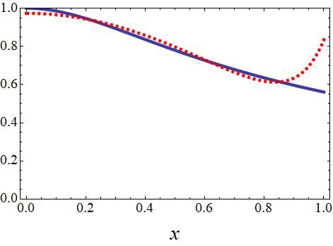
Figure 2: Comparison between the function $\Pi(x,Q^{2})$ at $Q^{2}=0.38$ GeV² (blue solid line) and $\Lambda_{\mathrm{tot}}(x)$ (red dashed line) defined in Eq. (27).

We shall end by commenting on the required level of precision for lattice calculations. We take the $\gamma W$ box as an example: in Ref. Seng et al. (2018b), the contribution from multiparticle intermediate states at $Q^{2}\sim 1$ GeV² to $\Delta_{R}^{V}$ is estimated to be $(\alpha/\pi)\times(0.48\pm 0.07)$ through a simple Regge-exchange model, with a $\sim 15\%$ error coming from the $\nu p/\bar{\nu}p$ scattering data. Possible systematic errors due to the simplicity of the model itself are not accounted for. In this sense, a successful lattice calculation of the second-order nucleon energy shift at a few points of $\omega$ with a precision level of $15\%$ will already be able to match the precision of the model and start to challenge its accuracy. This is completely executable with current lattice techniques as a similar calculation for parity-even structure functions has already been performed in Ref. Chambers et al. (2017b) with a 10% overall projected error. Also, by employing a larger $L$ one is able to probe smaller $Q^{2}$, and when sufficiently many points of $M_{1}[F_{3}^{N}]$ between $0.1$ GeV${}^{2}<Q^{2}<1$ GeV² are determined, one will be able to reduce the hadronic uncertainties in the $\gamma W$ and $\gamma Z$ boxes to a level compatible with current and future precision experiments.

Acknowledgements – The authors thank Akaki Rusetsky, Gerrit Schierholz and Mikhail Gorchtein for inspiring discussions. This work is supported in part by the DFG (Grant No. TRR110) and the NSFC (Grant No. 11621131001) through the funds provided to the Sino-German CRC 110 “Symmetries and the Emergence of Structure in QCD”, by the Alexander von Humboldt Foundation through a Humboldt Research Fellowship (CYS), by the Chinese Academy of Sciences (CAS) President’s International Fellowship Initiative (PIFI) (grant no. 2018DM0034) (UGM) and by VolkswagenStiftung (grant no. 93562) (UGM).

References

- Hardy and Towner (2015) J. C. Hardy and I. S. Towner, Phys. Rev. C91, 025501 (2015), eprint 1411.5987.
- Hardy and Towner (2018) J. C. Hardy and I. S. Towner, in 13th Conference on the Intersections of Particle and Nuclear Physics (CIPANP 2018) Palm Springs, California, USA, May 29-June 3, 2018 (2018), eprint 1807.01146.
- Kumar et al. (2013) K. S. Kumar, S. Mantry, W. J. Marciano, and P. A. Souder, Ann. Rev. Nucl. Part. Sci. 63, 237 (2013), eprint 1302.6263.
- Sirlin (1978) A. Sirlin, Rev. Mod. Phys. 50, 573 (1978), [Erratum: Rev. Mod. Phys. 50, 905 (1978)].
- Marciano and Sirlin (1983) W. J. Marciano and A. Sirlin, Phys. Rev. D27, 552 (1983).
- Marciano and Sirlin (1984) W. J. Marciano and A. Sirlin, Phys. Rev. D29, 75 (1984), [Erratum: Phys. Rev. D31, 213 (1985)].
- Marciano and Sirlin (1986) W. J. Marciano and A. Sirlin, Phys. Rev. Lett. 56, 22 (1986).
- Bardin et al. (2001) D. Yu. Bardin, P. Christova, L. Kalinovskaya, and G. Passarino, Eur. Phys. J. C22, 99 (2001), eprint hep-ph/0102233.
- Marciano and Sirlin (2006) W. J. Marciano and A. Sirlin, Phys. Rev. Lett. 96, 032002 (2006), eprint hep-ph/0510099.
- Gorchtein and Horowitz (2009) M. Gorchtein and C. J. Horowitz, Phys. Rev. Lett. 102, 091806 (2009), eprint 0811.0614.
- Gorchtein et al. (2011) M. Gorchtein, C. J. Horowitz, and M. J. Ramsey-Musolf, Phys. Rev. C84, 015502 (2011), eprint 1102.3910.
- Blunden et al. (2011) P. G. Blunden, W. Melnitchouk, and A. W. Thomas, Phys. Rev. Lett. 107, 081801 (2011), eprint 1102.5334.
- Rislow and Carlson (2013) B. C. Rislow and C. E. Carlson, Phys. Rev. D88, 013018 (2013), eprint 1304.8113.
- Seng et al. (2018a) C.-Y. Seng, M. Gorchtein, H. H. Patel, and M. J. Ramsey-Musolf, Phys. Rev. Lett. 121, 241804 (2018a), eprint 1807.10197.
- Seng et al. (2018b) C. Y. Seng, M. Gorchtein, and M. J. Ramsey-Musolf (2018b), eprint 1812.03352.
- Gorchtein (2018) M. Gorchtein (2018), eprint 1812.04229.
- Lin et al. (2018) H.-W. Lin et al., Prog. Part. Nucl. Phys. 100, 107 (2018), eprint 1711.07916.
- (18) R. P. Feynman, Phys. Rev. 56, 340 (1939).
- (19) H. Hellmann, Einführung in die Quantenchemie, Deuticke, Leipzig und Wien (1937).
- Chambers et al. (2017a) A. J. Chambers et al. (QCDSF, UKQCD, CSSM), Phys. Rev. D96, 114509 (2017a), eprint 1702.01513.
- Agadjanov et al. (2017) A. Agadjanov, U.-G. Meißner, and A. Rusetsky, Phys. Rev. D95, 031502 (2017), eprint 1610.05545.
- Agadjanov et al. (2019) A. Agadjanov, U.-G. Meißner, and A. Rusetsky, Phys. Rev. D99, 054501 (2019), eprint 1812.06013.
- Chambers et al. (2017b) A. J. Chambers, R. Horsley, Y. Nakamura, H. Perlt, P. E. L. Rakow, G. Schierholz, A. Schiller, K. Somfleth, R. D. Young, and J. M. Zanotti, Phys. Rev. Lett. 118, 242001 (2017b), eprint 1703.01153.
- (24) J. Ruiz de Elvira, U.-G. Meißner, A. Rusetsky and G. Schierholz, Eur. Phys. J. C 77, no. 10, 659 (2017).
- Nachtmann (1973) O. Nachtmann, Nucl. Phys. B63, 237 (1973).
- Nachtmann (1974) O. Nachtmann, Nucl. Phys. B78, 455 (1974).
- Erler et al. (2003) J. Erler, A. Kurylov, and M. J. Ramsey-Musolf, Phys. Rev. D68, 016006 (2003), eprint hep-ph/0302149.
- Becker et al. (2018) D. Becker et al., Eur. Phys. J. A54, 208 (2018), eprint 1802.04759.
- Bolognese et al. (1983) T. Bolognese, P. Fritze, J. Morfin, D. H. Perkins, K. Powell, and W. G. Scott (Aachen-Bonn-CERN-Democritos-London-Oxford-Saclay), Phys. Rev. Lett. 50, 224 (1983).
- Kataev and Sidorov (1994) A. L. Kataev and A. V. Sidorov, in ’94 QCD and high-energy hadronic interactions. Proceedings, Hadronic Session of the 29th Rencontres de Moriond, Moriond Particle Physics Meeting, Meribel les Allues, France, March 19-26, 1994 (1994), pp. 189–198, eprint hep-ph/9405254, URL https://inspirehep.net/record/37980/files/arXiv:hep-ph_9405254.pdf.
- Kim et al. (1998) J. H. Kim et al., Phys. Rev. Lett. 81, 3595 (1998), eprint hep-ex/9808015.
- Bouchard et al. (2017) C. Bouchard, C. C. Chang, T. Kurth, K. Orginos, and A. Walker-Loud, Phys. Rev. D96, 014504 (2017), eprint 1612.06963.
- (33) L. Liu et al., Phys. Rev. D 96 (2017) no.5, 054516.
- (34) M. Lüscher, EPJ Web Conf. 175 (2018) 01002.