Quasilinear Approach of the Whistler Heat-Flux Instability in the Solar Wind

Abstract

The hot beaming (or strahl) electrons responsible for the main electron heat-flux in the solar wind are believed to be self-regulated by the electromagnetic beaming instabilities, also known as the heat-flux instabilities. Here we report the first quasi-linear theoretical approach of the whistler unstable branch able to characterize the long-term saturation of the instability as well as the relaxation of the electron velocity distributions. The instability saturation is not solely determined by the drift velocities, which undergo only a minor relaxation, but mainly from a concurrent interaction of electrons with whistlers that induces (opposite) temperature anisotropies of the core and beam populations and reduces the effective anisotropy. These results might be able to (i) explain the low intensity of the whistler heat-flux fluctuations in the solar wind (although other explanations remain possible and need further investigation), and (ii) confirm a reduced effectiveness of these fluctuations in the relaxation and isotropization of the electron strahl and in the regulation of the electron heat-flux.

1 Introduction

Guided by the interplanetary magnetic field the electron beaming or strahl population carries the main electron heat flux in the solar wind (Feldman et al., 1975; Lin, 1998; Pierrard et al., 2001). At large distances from the Sun in-situ measurements reveal a significant inhibition of the electron heat flux (Gary et al., 1999; Scime et al., 1994; Bale et al., 2013) below the Spitzer–Härm predictions (Spitzer & Härm, 1953). Particle-particle collisions are rare and inefficient at large heliocentric distances, but the heat-flux can be regulated by the self-generated instabilities, through the wave-particle interactions. The observations support this hypothesis, showing evidences of enhanced electromagnetic fluctuations usually associated with the heat-flux instabilities (Scime et al., 1994; Gary et al., 1999; Pagel et al., 2007; Bale et al., 2013; Lacombe et al., 2014). Numerical simulations confirm a potential role of these instabilities in the regulation of electron heat-flux in the solar wind (Vocks et al., 2005; Saito & Gary, 2007; Roberg-Clark et al., 2018).

Heat-flux instabilities can manifest either as a whistler growing mode or as a firehose-like instability (Gary, 1985; Saeed et al., 2017a, b; Shaaban et al., 2018a, b), but such a distinction, although useful, is not always taken into account in specific studies of these instabilities. Here we focus on the whistler heat-flux instability, predicted by the linear theory for less energetic beams, i.e., with drifting velocity lower than thermal speed (Gary, 1985; Gary et al., 1999; Saeed et al., 2017a; Shaaban et al., 2018b; Tong et al., 2018), and often invoked to explain the enhanced fluctuations observed in the slow and moderate winds, e.g., with $v_{SW}<500$ km/s (Pagel et al., 2007; Lacombe et al., 2014; Stansby et al., 2016; Tong et al., 2019). These fluctuations may pitch-angle scatter the strahl, which becomes broader as electron energy increases and reduces in intensity with heliocentric distance (Maksimovic et al., 2005; Vocks et al., 2005; Pagel et al., 2007), explaining thus the inhibition of the electron heat flux in the solar wind (Gary, 1985; Tong et al., 2018; Tong et al., 2019).

Whistler waves (also known as electromagnetic electron cyclotron modes) are observed propagating at small angles along the interplanetary magnetic field with a right-handed circular polarization and frequency between ion and electron gyrofrequencies, i.e. $\Omega_{p}<\omega<|\Omega_{e}|$ (Wilson III et al., 2013; Lacombe et al., 2014). Local sources of whistlers are multiple, either the heat-flux instability driven by counter-beaming electrons (Feldman et al., 1973; Gary, 1993; Shaaban et al., 2018b), or the cyclotron instability driven by electrons with anisotropic temperatures, i.e., $T_{\perp}>T_{\parallel}$, where $\parallel,\perp$ denote directions with respect to the magnetic field (Gary & Wang, 1996; Lazar et al., 2018), or even the interplay of these two instabilities (Shaaban et al., 2018a). Both sources of free energy may indeed co-exist in space plasmas (Štverák et al., 2008; Viñas et al., 2010; Lazar et al., 2017), and recent studies (Saeed et al., 2017b; Shaaban et al., 2018b, a) have unveiled new regimes of whistler heat-flux instability in an attempt to provide an extended linear description in the solar wind conditions.

In the present paper we provide valuable physical insights from a quasilinear (QL) approach of the whistler heat-flux instability, which enable decoding of the main mechanisms leading to the saturation of the growing fluctuations and the relaxation of the electron counter-beaming distribution. As already mentioned, this instability involves less energetic beams and, implicitly, low-level growth-rates and fluctuations which are not easily captured in the simulations. In this context, a quasilinear approach can offer unique methods to investigate the long-term evolution of this instability and its actions back on the electron velocity distribution. Quasilinear approaches have been successfully employed in studies of both the whistler and firehose instabilities driven by the temperature anisotropy, and the results showed agreements with the linear theory predictions, particle-in-cell simulations, and the observational limits of the electron temperature anisotropy (Yoon et al., 2012; Seough et al., 2014, 2015; Yoon et al., 2017; Lazar et al., 2018; Shaaban et al., 2019).

The manuscript is structured as follows: In section 2 we introduce the particle velocity distribution functions (VDFs), with a focus on the counter-drifting (dual) core-beam model for the electrons. This model describes the counter-moving of the core and beam populations in terms of their drifting velocities, i.e. $U_{c}$ and $U_{b}$, respectively, which act as a source of free energy triggering different instabilities. Both linear and QL theoretical formalisms for dispersion and stability are are described in section 3. In section 4 we present an extended analysis of the unstable whistler heat-flux solutions for three cases with potential implications in the regulation of the electron strahl and the electron heat flux in the solar wind. The results obtained in the present work are summarized in section 5.

2 Counter-drifting solar wind electron distribution

Solar wind in-situ measurements, e.g., from various spacecraft missions, e.g., Helios 1, Cluster II, Ulysses, or Wind, reveal electron distributions with a dual structure combining two counter-drifting components in a frame fixed to protons, namely, a thermal and dense core and a strahl population streaming along the magnetic field (Gary et al., 1999; Maksimovic et al., 2005; Tong et al., 2019).

$$f_{e}\left(v_{\parallel},v_{\perp}\right)=\dfrac{n_{c}}{n_{0}}~{}f_{c}\left(v_{\parallel},v_{\perp}\right)+\dfrac{n_{b}}{n_{0}}~{}f_{b}\left(v_{\parallel},v_{\perp}\right).$$ (1)

where $n_{c}$ and $n_{b}$ are the core and beam number density, respectively, and $n_{0}$ is the total number density of electrons. Quasilinear approach is not straightforward, but for the sake of simplicity, here we assume both the core (subscript $c$) and beam (subscript $b$) components well described by drifting bi-Maxwellian models (Shaaban et al., 2018a)

$$f_{a}\left(v_{\parallel},v_{\perp}\right)= \frac{1}{\pi^{3/2}\alpha_{\perp a}^{2}~{}\alpha_{\parallel a}}\exp\left(-\frac{v_{\perp}^{2}}{\alpha_{\perp a}^{2}}-\frac{\left(v_{\parallel}-U_{a}\right)^{2}}{\alpha_{\parallel a}^{2}}\right)$$ (2)

where thermal velocities $\alpha_{\parallel,\perp,a}\equiv\alpha_{\parallel,\perp,a}(t)$ are defined in terms of the corresponding kinetic temperature components, which may evolve in time ($t$)

$$T_{\parallel,a} =\frac{m_{e}}{k_{B}}\int d\textbf{v}~{}(v_{\parallel}-U_{a})^{2}~{}f_{a}(v_{\parallel},v_{\perp})=\frac{m_{e}~{}\alpha_{\parallel,a}^{2}}{2k_{B}},$$ (3a)

$$T_{\perp,a} =\frac{m_{e}}{2k_{B}}\int d\textbf{v}~{}v_{\perp}^{2}~{}f_{a}(v_{\parallel},v_{\perp})=\frac{m_{e}~{}\alpha_{\perp,a}^{2}}{2k_{B}},$$ (3b)

$U_{a}$ is drifting velocity, either for the core (subscript "$a=c$") or beam (subscript "$a=b$"), along the background magnetic field. We perform our analysis in a quasi-neutral electron-proton plasma $n_{e}=n_{c}+n_{b}\approx n_{p}$, with zero net current, i.e. $n_{c}~{}U_{c}+n_{b}~{}U_{b}=0$.

3 Quasilinear instability approach

For a collisionless and homogeneous plasma the linear dispersion relation derived from kinetic theory for the right-handed (RH) circularized polarized electromagnetic modes propagating in directions parallel to the stationary magnetic field (${\bf k}\times{\bf B}_{0}=0$) reads (Shaaban et al., 2018a)

$$\tilde{k}^{2}= (1-\delta)~{}\mu~{}\left[\Lambda_{c}+\frac{(\Lambda_{c}+1)~{}(\tilde{\omega}-\tilde{k}~{}u_{c})-\mu~{}\Lambda_{c}}{\tilde{k}\sqrt{\mu~{}\beta_{c}}}\right.$$

$$\left.\times Z_{c}\left(\frac{\tilde{\omega}-\mu-\tilde{k}~{}u_{c}}{\tilde{k}\sqrt{\mu~{}\beta_{c}}}\right)\right]+\frac{\tilde{\omega}}{\tilde{k}~{}\sqrt{\beta_{p}}}Z_{p}\left(\frac{\tilde{\omega}+1}{\tilde{k}\sqrt{\beta_{p}}}\right)$$

$$+\delta~{}\mu\left[\Lambda_{b}+\frac{(\Lambda_{b}+1)~{}(\tilde{\omega}-\tilde{k}~{}u_{b})-\mu~{}\Lambda_{b}}{\tilde{k}\sqrt{\mu~{}\beta_{b}}}\right.$$

$$\left.\times Z_{b}\left(\frac{\tilde{\omega}-\mu-\tilde{k}~{}u_{b}}{\tilde{k}\sqrt{\mu~{}\beta_{b}}}\right)\right]$$ (4)

where $\tilde{k}=kc/\omega_{p,p}$ is the normalization used for wave-number $k$, $c$ is the speed of light, $\omega_{p,p}~{}=~{}\sqrt{4\pi n_{0}e^{2}/m_{p}}$ is the plasma frequency of protons, $\tilde{\omega}=\omega/\Omega_{p}$ is the normalization for wave frequency, $\Omega_{p}$ is the non-relativistic gyro-frequency of protons, $\mu=m_{p}/m_{e}$ is the proton–electron mass contrast, $\Lambda_{a}=~{}T_{\perp,a}/T_{\parallel,a}-~{}1\equiv A_{a}-1$ and $\beta_{\parallel,\perp,a}=8\pi n_{0}k_{B}T_{\parallel\perp,a}/B_{0}^{2}$ are, respectively, the temperature anisotropy, and plasma beta parameters for protons (subscript "$a=p$"), electron core (subscript "$a=c$"), and electron beam (subscript "$a=b$") populations, $\delta=n_{b}/n_{0}$, $1-\delta=n_{c}/n_{0}$ are the beam and core relative densities, respectively, $u_{a}=U_{a}/v_{A}$ are normalized drifting velocities, $v_{A}=\sqrt{B_{0}^{2}/4\pi n_{p}m_{p}}$ is the proton Alfvén speed, and

$$Z_{a}\left(\xi_{a}^{\pm}\right)=\frac{1}{\sqrt{\pi}}\int_{-\infty}^{\infty}\frac{\exp\left(-x^{2}\right)}{x-\xi_{a}^{\pm}}dt,\ \ \Im\left(\xi_{a}^{\pm}\right)>0,$$ (5)

are plasma dispersion functions (Fried & Conte, 1961).

In the quasilinear formalism one must solve for both particle and wave kinetic equations. For parallel propagation of electromagnetic waves, the particle kinetic equation in the diffusion approximation describes the time evolution of the velocity distributions as follows

$$\frac{\partial f_{a}}{\partial t} =\frac{ie^{2}}{4m_{a}^{2}c^{2}~{}v_{\perp}}\int_{-\infty}^{\infty}\frac{dk}{k}\left[\left(\omega^{\ast}-kv_{\parallel}\right)\frac{\partial}{\partial v_{\perp}}+kv_{\perp}\frac{\partial}{\partial v_{\parallel}}\right]$$

$$\times~{}\frac{v_{\perp}\delta B^{2}(k,\omega)}{\omega-kv_{\parallel}-\Omega_{a}}\left[\left(\omega-kv_{\parallel}\right)\frac{\partial f_{a}}{\partial v_{\perp}}+kv_{\perp}\frac{\partial f_{a}}{\partial v_{\parallel}}\right]$$ (6)

where $\delta B^{2}(k)$ is the energy density of the fluctuations. The wave equation is given by

$$\frac{\partial~{}\delta B^{2}(k)}{\partial t}=2\gamma_{k}\delta B^{2}(k),$$ (7)

with growth rate $\gamma_{k}$ of the unstable whistler solutions obtained from Eq. (3). Dynamical equations for the macroscopic moments of the veocity distribution, such that the drift velocities $U_{a}$ of core (subscript "$a=c$") and beam (subscript "$a=b$"), and their temperature components $T_{\perp,\parallel,a}$ are derived from Eq. (3) as follows

$$\frac{dU_{c}}{dt} =\frac{e^{2}m_{e}^{-2}}{2~{}c^{2}}\int_{-\infty}^{\infty}\frac{dk}{k}\langle~{}\delta B^{2}(k)~{}\rangle\text{Im}\left\{\eta_{c}~{}Z_{c}\left(\zeta_{c}\right)\right\}$$ (8a)

$$\frac{dU_{b}}{dt} =\frac{e^{2}m_{e}^{-2}}{2~{}c^{2}}\int_{-\infty}^{\infty}\frac{dk}{k}\langle~{}\delta B^{2}(k)~{}\rangle\text{Im}\left\{\eta_{h}~{}Z_{b}\left(\zeta_{b}\right)\right\}$$ (8b)

$$\frac{dT_{\perp a}}{dt} =-\frac{e^{2}}{2m_{e}c^{2}}\int_{-\infty}^{\infty}\frac{dk}{k^{2}}\langle~{}\delta B^{2}(k)~{}\rangle$$

$$\times\left\{\left(2\Lambda_{c}+1\right)\gamma_{k}+\text{Im}\left(2i\gamma-\Omega_{e}\right)~{}\eta_{a}Z_{a}\left(\zeta_{a}\right)\right\}$$ (8c)

$$\frac{dT_{\parallel a}}{dt} =\frac{e^{2}}{m_{e}c^{2}}\int_{-\infty}^{\infty}\frac{dk}{k^{2}}\langle~{}\delta B^{2}(k)~{}\rangle$$

$$\times\left\{2\left(\Lambda_{a}+1\right)\gamma_{k}+\text{Im}~{}k~{}\alpha_{\parallel a}~{}\zeta_{a}~{}\eta_{a}Z_{a}\left(\zeta_{a}\right)\right\}$$ (8d)

with

$$\eta_{c}=\left[\left(\Lambda_{c}+1\right)\left(\omega-k~{}U_{c}\right)-\Omega_{e}~{}\Lambda_{c}\right]/\left(k~{}\alpha_{\parallel c}\right),$$

$$\eta_{b}=\left[\left(\Lambda_{b}+1\right)\left(\omega-k~{}U_{b}\right)-\Omega_{e}~{}\Lambda_{b}\right]/\left(k~{}\alpha_{\parallel b}\right),$$

$$\zeta_{c}=\frac{\omega-\Omega_{e}-k~{}U_{c}}{k~{}\alpha_{\parallel c}}~{}~{}\&~{}~{}\zeta_{b}=\frac{\omega-\Omega_{e}-k~{}U_{b}}{k~{}\alpha_{\parallel b}}.$$

As above in Eq. (3), we can use normalized quantities

$$\tilde{\eta}_{c}=\left[\left(\Lambda_{c}+1\right)\left(\tilde{\omega}-\tilde{k}~{}u_{c}\right)-\mu~{}\Lambda_{c}\right]/\left(\tilde{k}~{}\sqrt{\mu~{}\beta_{\parallel c}}\right),$$

$$\tilde{\eta}_{b}=\left[\left(\Lambda_{b}+1\right)\left(\tilde{\omega}-\tilde{k}~{}u_{b}\right)-\mu~{}\Lambda_{b}\right]/\left(\tilde{k}~{}\sqrt{\mu~{}\beta_{\parallel b}}\right),$$

$$\tilde{\zeta}_{c}=\frac{\tilde{\omega}-\mu-\tilde{k}~{}u_{c}}{\tilde{k}~{}\sqrt{\mu~{}\beta_{\parallel c}}},~{}~{}\tilde{\zeta}_{b}=\frac{\tilde{\omega}-\mu-\tilde{k}~{}u_{b}}{\tilde{k}~{}\sqrt{\mu~{}\beta_{\parallel b}}}$$

$$u_{b}=U_{b}/v_{A},~{}~{}u_{c}=U_{c}/v_{A},~{}~{}\tau=\Omega_{p}~{}t$$

and $W(\tilde{k})=\delta B^{2}(\tilde{k})/B_{0}^{2}$ (for the wave energy density), to find

$$\frac{du_{c}}{d\tau} =\mu^{2}\int_{\infty}^{\infty}\frac{d\tilde{k}}{\tilde{k}}W\left(\tilde{k}\right)\text{Im}\left\{\tilde{\eta}_{c}Z_{c}\left(\tilde{\zeta}_{c}\right)\right\}$$ (9a)

$$\frac{du_{b}}{d\tau} =\mu^{2}\int_{-\infty}^{\infty}\frac{d\tilde{k}}{\tilde{k}}W\left(\tilde{k}\right)\text{Im}\left\{\tilde{\eta}_{b}Z_{h}\left(\tilde{\zeta}_{b}\right)\right\}$$ (9b)

$$\frac{d\beta_{\perp a}}{d\tau} =-2\mu\int_{-\infty}^{\infty}\frac{d\tilde{k}}{\tilde{k}^{2}}~{}W\left(\tilde{k}\right)$$

$$\times\left\{\left(2\Lambda_{c}+1\right)\tilde{\gamma}_{k}+\text{Im}\left(2i\tilde{\gamma}-\mu\right)\tilde{\eta}_{a}Z_{a}\left(\tilde{\zeta}_{a}\right)\right\}$$ (9c)

$$\frac{d\beta_{\parallel a}}{d\tau} =4\mu\int_{-\infty}^{\infty}\frac{d\tilde{k}}{\tilde{k}^{2}}~{}W\left(\tilde{k}\right)$$

$$\times\left\{2\left(\Lambda_{c}+1\right)\tilde{\gamma}_{k}+\text{Im}~{}\tilde{k}\sqrt{\mu~{}\beta_{\parallel a}}~{}\tilde{\zeta}_{a}\tilde{\eta}_{a}Z_{a}\left(\tilde{\zeta}_{a}\right)\right\}$$ (9d)

and

$$\frac{\partial~{}W(\tilde{k})}{\partial\tau}=2~{}\tilde{\gamma}~{}W(\tilde{k}).$$ (10)

If both the core and beam populations are assumed drifting bi-Maxwellian the heat flux is given by (Gary et al., 1994)

$$q_{e}=\dfrac{m_{e}}{2}\sum_{a=c,b}n_{a}U_{a}\left[\left(3+2\dfrac{T_{\perp a}}{T_{\parallel a}}\right)\alpha_{\parallel a}^{2}+U_{a}^{2}\right]$$ (11)

or normalized

$$\dfrac{q}{q_{max}}=\left(1-\delta\right)\dfrac{|u_{c}|}{\sqrt{\mu\beta_{\parallel c}}}\left[\left(\dfrac{\beta_{\parallel b}}{\beta_{\parallel c}}-1\right)+\dfrac{2}{3}\left(\dfrac{\beta_{\perp b}}{\beta_{\perp c}}-1\right)\dfrac{\beta_{\perp c}}{\beta_{\parallel c}}\right],$$ (12)

using $q_{max}=3n_{0}T_{\parallel c}\alpha_{\parallel c}/2$. For isotropic temperatures $\beta_{\perp}=\beta_{\parallel}$, and Eq.(12) reduces to

$$\dfrac{q}{q_{max}}=\dfrac{5}{3}~{}\left(1-\delta\right)~{}\dfrac{|u_{c}|}{\sqrt{\mu~{}\beta_{\parallel c}}}\left(\dfrac{\beta_{\parallel b}}{\beta_{\parallel c}}-1\right),$$ (13)

4 Numerical results

In this section we discuss the numerical results from the linear and QL analysis of the unstable whistler heat flux mode triggered by the core-beam counterstreaming electrons. Details are presented for three distinct cases corresponding to conditions typically encountered in the solar wind (Maksimovic et al., 2005; Tong et al., 2018), with the following plasma parameters:

1. Case 1.

   $$U_{b}(0)=40~{}v_{A},\text{and}~{}U_{c}(0)=-2.1~{}v_{A}$$

   $$\beta_{c}(0)=1,~{}2,~{}3,\text{and}~{}T_{b}(0)=6~{}T_{c}(0),$$

   $$A_{c,b}(0,\tau_{max})=\frac{\beta_{\perp,c,b}(0,\tau_{max})}{\beta_{\parallel,c,b}(0,\tau_{max})}=1.0,$$ (14)

2. Case 2.

   $$U_{b}(0)/v_{A}=60,~{}40,~{}20,$$

   $$U_{c}(0)/v_{A}=-3.1,~{}-2.1,~{}-1.0,$$

   $$\beta_{c}(0)=2,\text{and}~{}T_{b}(0)=6~{}T_{c}(0),$$

   $$A_{c,b}(0,\tau_{max})=\frac{\beta_{\perp,c,b}(0,\tau_{max})}{\beta_{\parallel,c,b}(0,\tau_{max})}=1.0,$$ (15)

3. Case 3.

   $$U_{b}(0)=40~{}v_{A},\text{and}~{}U_{c}(0)=-2.1~{}v_{A}$$

   $$\beta_{c}(0)=3,\text{and}~{}T_{b}(0)=6~{}T_{c}(0),$$

   $$A_{c,b}(0)=\frac{\beta_{\perp,c,b}(0)}{\beta_{\parallel,c,b}(0)}=1.0.$$ (16)

Other plasma parameters used in our numerical computations are $\delta=0.05$, $W(k)=5\times 10^{-6}$ $\omega_{p,e}/|\Omega_{e}|=100$ and $v_{A}=2\times 10^{-4}~{}c$.

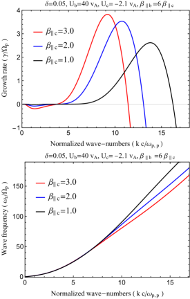
Figure 1: Wave-number dispersion of whistler heat flux growth rates (top) and wave-frequencies (bottom) and their variation with plasma beta.

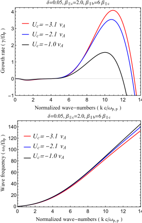
Figure 2: Wave-number dispersion of whistler heat flux growth rates (top) and wave-frequencies (bottom) and their variation with core drift velocity.

4.1 Linear Analysis

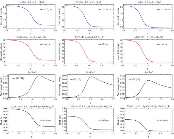
Figure 3: Case 1: QL time evolution of the drift velocities for core ($U_{c}$) and beam electrons ($U_{b}$), the wave energy density ($\delta B(t)/B_{0}^{2}$), and the heat flux ($q_{e}/q_{max}$) for different initial conditions: $\beta_{c}(0)=1$ (left), $2$ (middle), $3$ (right).

For a linear analysis we solve numerically the wavenumber dispersion relation (5). In Figure 1 we study the effect of the core plasma beta $\beta_{\parallel c}=1,2,3$ on the dispersive characteristics of the WHF instability, i.e., growth rate (top panel) and wave frequency (bottom panel), using the plasma parameters in case 1. The instability growth rate increases as the core plasma beta increases, but the range of the unstable wavenumbers decreases and the WHF instability becomes more effective at lower wavenumbers. The corresponding wave frequencies are decreasing with increasing the core plasma beta. For case 2. the unstable WHF solutions are displayed in Figure 2 enabling us to compare the instability growth rates (top panel) and wave frequencies (bottom panel) for different core drift velocities $u_{c}=-3.1,~{}-2.1,~{}-1.0$ (implying different velocities for the beam component $u_{b}=60,~{}40,~{}20$). The growth rates are increasing with increasing the core drift velocity, while the corresponding wave frequencies are slightly decreasing. However, for $\beta_{\parallel c}=2.0$ and $u_{c}=-3.1$ the WHF achieves its maximum growth rate and any further increase in the drift velocity inhibits the growth rate. Shaaban et al. (2018b, a) have described in detail this non-uniform variation of the growth rates as a function of the drift velocity, showing that growth rates of WHF branch are conditioned by the thermal velocity of the resonant beaming electrons, satisfying $v_{res}\gtrsim u_{b}$. Moreover, increasing the drift velocity and plasma beta induces a transition regime of interplay of both WHF and firehose-like branches of HF instability.

4.2 Quasilinear Analysis

Quasilinear (QL) analysis allows us to follow and understand temporal evolution of the enhanced fluctuations, i.e., the increase of the wave energy density $\delta B(t)/B_{0}^{2}$ up to the saturation, as well as the reaction of these fluctuations back on the VDFs of plasma particles, describing their relaxation and, eventually, their thermalization. To do so, we solve the the set of QL equations (9) and (10) for three distinct sets of plasma parameters, as mentioned above as cases 1, 2 and 3.

4.2.1 Case 1

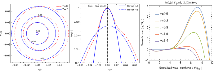
Figure 4: Case 1: Contours (left) and parallel cuts (middle) of electron velocity distribution ($\beta_{c,\parallel}=1$), initially ($\tau=0$) and after $\tau=2$; WHF growth rates for $\beta_{c,\parallel}=3$ (right) at different times relevant for the evolutions in Figure 3, right panels.

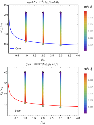
Figure 5: Case 1: dynamical decreasing paths for the core and beam electrons in ($u_{a},~{}\beta_{\parallel c}$)$-$space, whose initial states are shown with black circles. Final positions after saturation are indicated with gray circles, and the magnetic wave energy level is color-coded.

In case 1 we assume different initial conditions as given by different values of $\beta_{\parallel c}(0)$ (implying different $\beta_{\parallel b}=6~{}\beta_{\parallel c}$), and study the evolution of the fluctuating power and the main drivers of the instability, i.e., drift velocities of core and beaming electrons, by assuming that their temperature anisotropies do not change in time and remain isotropic, i.e., $A_{c,b}(\tau)=1.0$. Thus, Figure 3 displays temporal evolution of the drift velocities for the core ($U_{c}$) and beam ($U_{b}$), the wave energy density ($\delta B(t)/B_{0}^{2}$), and the heat flux ($q_{e}/q_{max}$) as functions of the normalized time $\tau=\Omega_{p}t$ and for different initial conditions: $\beta_{c}(0)=1$ (left), $2$ (middle), $3$ (right). Both components are relaxed, as their relative drifts are both reduced in time, up to the saturation of the instability, when the enhanced fluctuating power starts diminishing. An increase of the initial $\beta_{c}(0)$ accelerates these mechanisms, but reduces the effective anisotropy (Shaaban et al., 2018a) leading to lower drifts and lower levels of fluctuations after saturation. Bottom panels show the decrease of heat flux with similar time profiles.

Figure 4 displays contours (left) and parallel cuts (middle) of the electron distributions at initial and final times, i.e. $\tau=0$ (red-dotted) and $2$ (blue-solid), respectively, for $\beta_{\parallel c}(0)=1$ corresponding to the results in Figure 3, left panels. For both snapshots contour levels represent $10^{-3}$, $10^{-2}$, $0.045$, and $0.95$ of $f_{e,max}=1$. It is obvious that after the saturation of the WHF instability, e.g. at $\tau=2$, the drift velocities are both very low and the VDF is stable. This reduction of the relative drift velocities at later times ($\tau=2$) is more apparent in middle panel showing the parallel cuts of the electron distributions. Moreover, right panel displays the WHF growth rates for $\beta_{\parallel c}(0)=3$ (corresponding to the results in Figure 3, right panels), at intermediary time steps. As expected, these growth rates decrease due to a decrease of the drift velocities in time. The variation of the wave frequency is negligible (not shown here).

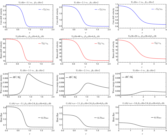
Figure 6: Case 2: QL time evolution of the drift velocities for core ($U_{c}$) and beam electrons ($U_{b}$), the wave energy density ($\delta B(t)/B_{0}^{2}$), and the heat flux ($q_{e}/q_{max}$) for different initial conditions: $U_{c}=-3.1~{}v_{A}$ (left), $U_{c}=-2.1~{}v_{A}$ (middle), $U_{c}=-1.0~{}v_{A}$ (right).

Dynamical paths of the drift velocities $U_{a}/v_{a}$ as a function of $\beta_{\parallel c}$ are displayed in Figure 5, for both the core ($"a=c"$, top panel), and beam ($"a=b"$, bottom panel). Black circles indicate initial positions, while gray circles mark final states after saturation. The variation of magnetic wave energy $\delta B^{2}/B_{0}^{2}$ is color coded. The final states of the dynamical paths end up very close to the instability thresholds, i.e., the lowest drift velocities predicted by the linear theory (unstable regimes are situated above the thresholds). These temporal profiles clearly show the relaxations of the core and beam drift velocities towards the most stable regime in agreement with the drift velocity thresholds predicted by the linear theory. These velocity thresholds are derived for a maximum growth rate $\gamma_{max}=0.27~{}\Omega_{p}\approx 1.5\times 10^{-4}|\Omega_{e}|$ , and are well fitted to (Shaaban et al., 2018a)

$$-U_{c}/v_{A}=\frac{s}{\beta_{\parallel~{}c}^{~{}\alpha}},~{}~{}~{}\&~{}~{}U_{b}/v_{A}=\frac{s}{\beta_{\parallel~{}c}^{~{}\alpha}}.$$ (17)

with ($s,~{}\alpha$) =  ($0.66,~{}0.30$) for the core ($a=c$) and ($s,~{}\alpha$) = ($12.47,~{}0.27$) for the beam ($a=b$) components.

4.2.2 Case 2

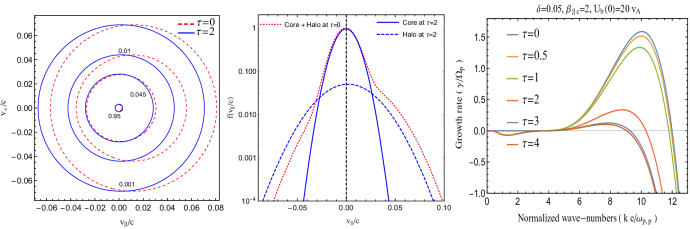
Figure 7: Case 2: Contours (left) and parallel cuts (middle) of electron velocity distribution ($U_{c}=-3.1~{}v_{A}$), initially ($\tau=0$) and at $\tau=2$; WHF growth rates for $U_{c}=-1.0~{}v_{A}$ (right) at different times relevant for the evolutions in Figure 6, right panels.

Here our QL analysis starts from different conditions, assuming initially three different core drift velocities $U_{c}/v_{A}=-3.1,~{}-2.1,~{}-1$ (implying different beaming velocity $U_{b}/v_{A}=60,~{}40,~{}20$). Figure 6 shows time evolution for the drift velocities of the core ($U_{c}$) and beam ($U_{b}$), the corresponding time variation of the wave energy density ($\delta B^{2}/B_{0}^{2}$) and the normalized heat flux ($q_{e}/q_{max}$). We assume again that temperature anisotropy is not affected by the growing fluctuations. After the saturation the core and beam drift velocities end up to almost the same velocities, regardless the value of the the initial drift velocity. However, lower drift velocities, i.e. $U_{c}=-1.0~{}v_{A}$ and $U_{b}=20~{}v_{A}$, need longer time to relax. The associated wave energy density and the normalized heat flux increase with increasing the core drift velocity, confirming the enhancement of the WHF growth rates in Figure 2.

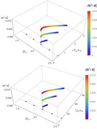
Figure 8: Case 2: 3D display dynamical paths of the drift velocities for the core (top) and beam (bottom), and the varying level of magnetic wave energy with colors . Initial states are shown with black circles, while final positions after saturation are indicated with gray circles which follow the profile of the instability thresholds at $\beta_{c,\parallel}=2$.

In Figure 7, contours (left panel) and parallel cuts (middle panel) represent the initial and final states (i.e. $\tau=0$ and $\tau=2$, respectively) of the eVDFs in the QL evolution of WHF instability for $U_{c}(0)=-3.1~{}v_{A}$, see also Figure 6. Initial drift velocities of the core and beam are regulated by the enhanced fluctuations, and distribution becomes less anisotropic and, therefore, more stable at $\tau=2$ (blue solid contours). Right panel displays the WHF growth rates for $U_{c}=-1.0~{}v_{A}$, for different times up to the saturation and after, corresponding to the results in Figure 6, left panels. These growth rates are decreasing in time coresponding to a decrease of the core and beam drift velocities, see Figure 6. The time variation of the wave frequency is negligible and is not shown here.

In case 2, comparison of the instability thresholds (predicted by the linear theory) and dynamical paths of the core and beam drift velocities from QL analysis is made for the same value of the core plasma beta, i.e. $\beta_{\parallel c}=2$, and is therefore less straightforward. Figure 8 displays 3D dynamical paths of the core and beam drift velocities in order to avoid their overlap. Threshold conditions are indicated by dotted lines in the horizontal plane $U_{a}/v_{A}-\beta_{c,\parallel}$, and final states align to the vertical line of drift velocities corresponding to maximum wave energy densities. Dynamical paths of the drift velocity for both core (top) and beam (bottom) end up very close to the instability threshold predicted by the linear theory at the same condition of saturation for the wave energy density.

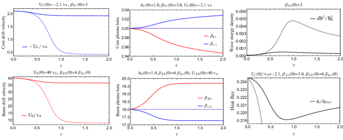
Figure 9: Case 3: QL time evolution of the drift velocities (left), plasma betas (middle), the wave energy density (top-right) and the heat flux (bottom-right) for $U_{c}=-2.1~{}v_{A}$ and $\beta_{c}=3.0$.

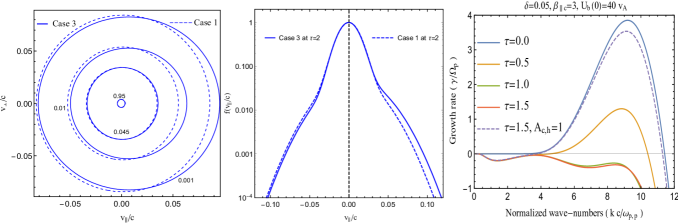
Figure 10: Case 3: Contours (left) and parallel cuts (middle) of electron velocity distribution, initially ($\tau=0$) and at $\tau=2$; WHF growth rates for $U_{c}=-1.0~{}v_{A}$ (right) at different times relevant for the evolutions in Figure 9.

4.2.3 Case 3

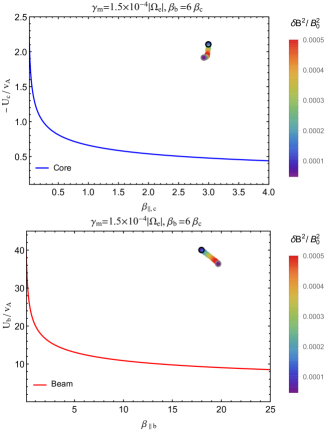
Figure 11: The same as Figure 5, but for case 3.

Suppose now, more realistically, that all plasma parameters, e.g., drift velocities ($u_{c,b}$), plasma beta parameters ($\beta_{c,b}$), may vary in time (i.e., normalized time $\tau=\Omega_{p}t$). Figure  9 presents, by comparison, time evolutions for the core and beam drift velocities (left panels), the plasma betas (middle panels), and the corresponding wave energy density (top-right) and heat flux (bottom-right) for an initial $\beta_{\parallel c}(0)=3.0$. Comparison includes cases 1 (dotted lines) and 3 (solid lines). Allowing electron temperatures and, implicitly, plasma betas to vary in time markedly reduces the relaxation of the core and beams drift velocities (solid lines) to values only slightly below the initial conditions but much higher than those obtained after relaxation in case 1 (dotted lines). However in this case temperatures do not remain isotropic, but change under the effect of enhanced WHF fluctuations leading to small deviations from isotropy. The core and beam components reach opposite temperature anisotropies after relaxation, as indicated by their parallel (red) and perpendicular (blue) plasma betas in middle panels. The core shows an excess of perpendicular temperature $A_{c}(\tau=2)=\beta_{\perp c}/\beta_{\parallel c}(\tau=2)=1.024$, while the beam shows an excess of parallel temperature $A_{b}(\tau=2)=\beta_{\perp b}/\beta_{\parallel b}=0.877$. Shaaban et al. (2018a) have indeed shown that WHF instability is markedly inhibited by such a temperature anisotropy of the beam, that may explain, comparing to case 1, the saturation at lower wave energy densities, a modest relaxation at higher drift velocities and a minor reduction of the heat-flux. The opposite anisotropies gained by the core and beam components can be explained by a series of selective mechanisms: (a) heating of the core electrons in perpendicular direction by resonant interactions with whistlers, (b) scattering and diffusion in velocity space of the beam electrons leading to a plateau formation and an effective temperature anisotropy $T_{b,\parallel}>T_{b,\perp}$.

In Figure 10, we display, for comparison, contours and parallel cuts of the eVDFs in the later stages after saturation, (i.e., $\tau=2$) for case 1 (dotted lines) with $\beta_{c\parallel}=3$ and case 3 (solid lines). These final states are markedly different, in case 3 we can still observe an anisotropic distribution drifting in parallel direction, while in case 1 it is more isotropic (and therefore more stable). Right-panel in Figure 10 shows the WHF growth rates for case 3 at different intermediary times. These growth rates decrease in time, and the WHF mode is damped at $\tau=1.5$. In order to understand the role played by the induced temperature anisotropies, e.g., in Figure 9 middle panels, with dashed line we add the WHF growth rate obtained for the same drifting velocities of the core and beam at $\tau=1.5$ but when temperatures of these populations are maintained constant and isotropic (similar to cases 1 and 2). This growth rate display a considerable peak, while for case 3 when the core exhibit $T_{c,\perp}>T_{c,\parallel}$ and the beam $T_{b,\perp}<T_{b,\parallel}$, WHF mode is damped. Allowing temperatures and implicitly plasma betas to vary in time inhibits the growth rates and leads to a faster saturation of the instability. Without artificial constraints to keep constant particle temperatures (or plasma beta parameters), the QL results seem to be more realistic than those obtained in cases 1 and 2, and suggest a new self-inhibiting effect of WHF instability. This saturation results from multiple effects combining a minor relaxation of drift velocities with a transverse heating of the (highly dense) core, and an additional (elastic) scattering of the beam (Marsch, 2006), which together contribute to a reduction of the effective anisotropy and inhibit the instability.

Opposite variations of parallel plasma beta parameters, towards lower values for the core (top) and higher values for the beam (bottom) are also shown in Figure 11 by the dynamical paths of the drift velocities for the core (top) and beam (bottom). However, in this case final states do not approach the instability thresholds predicted by the linear theory, which have no relevance in this case. This result demonstrates the importance of an extended QL approach of WHF instability, which can realistically unveil long-term evolution of the enhanced fluctuations with multiple effects on the velocity distributions of electrons (i.e., thermalization, cyclotron heating). Linear theory can predict only a reduction of the drift velocities towards lowest threshold values, but a QL approach may quantify additional transfers of energy between wave fluctuations and particles, as shown by the time evolutions of the higher order moments of the velocity distribution, e.g., temperatures and heat-flux.

5 Discussions and Conclusions

In the present paper we have characterized the quasilinear evolution of the whistler heat-flux instability driven by two counter-beaming Maxwellian electron populations, resembling the velocity distributions observed in the space plasmas. Central component is the highly dense core but the additional beaming or strahl population is mainly responsible for the electron heat-flux in the solar wind. The whistler heat-flux instability is selfgenerated when the relative beaming or drift velocity does not exceed thermal speed of beaming electrons. However, the main interest is to understand if growing fluctuations act back on the electron beams, reducing their anisotropy and regulating the heat-flux. Our present results from an extensive quasilinear study of the whistler heat-flux instability may offer valuable answers to these questions.

Section 4 presents the results of a parametric study on the influence of the initial conditions, i.e., macroscopic plasma parameters like drifting velocities and plasma beta parameters for the core and beam, on the saturation of this instability and the relaxation of the electron distribution. In the firsts two cases we have allowed only for time variations of the drift velocities (the source of free energy), while temperatures are kept constant. Higher plasma betas assumed initially for the core electrons (case 1) seem to stimulate the instability maximum growth rate in the linear phase, but restrain to range of unstable wave-numbers. Moreover, growing fluctuations become less robust saturating faster and at lower fluctuating field energy densities. The corresponding relaxations of counter-beams and the heat-flux are also faster leading to lower levels. In fact, particle thermalization is indeed expected to suppress beaming instabilities, but for the whistler heat-flux instability this effect becomes obvious only in the long term evolution. The influence of drifting velocity (case 2) is less controversial, e.g., higher values of $U_{c}$ enhance not only the growth-rates but markedly stimulate growing fluctuations to high energy densities, and implicitly, accelerates the inhibition of the drifts and the electron heat-flux. In both these two cases the saturated stage is described by more stationary distributions, which carry lower heat-flux, and approach, as expected, the drift velocity thresholds predicted by linear theory.

Case 3 is more realistic as we have enabled for time variations of all plasma parameters, i.e., temperatures and drift velocities, as may result from the interactions of electrons with growing fluctuations. The relaxation of the core and beams drift velocities is very modest in this case, to values only slightly below the initial conditions. However, temperatures also change leading to small deviations from isotropy, and opposite anisotropies of the core and beam components, which actually explains the faster inhibition of the instability (Shaaban et al., 2018a) and minor relaxation of the beam and the heat-flux. Triggered by the whistler fluctuations, these effects result from the concurrence of the core electrons heating by resonant interactions with whistlers, and elastic scattering of the beam electrons and their diffusion in velocity space leading to a plateau formation and an effective temperature anisotropy $T_{b,\parallel}>T_{b,\perp}$.

We can state that our QL approach in case 3 enables a number of clear conclusions. Linear theory cannot capture the energy transfer between the electron populations, and consequently cannot describe correctly the saturation of whistler heat flux instability and the relaxation of velocity distribution. It is QL theory that offers a more complete and realistic picture, showing that this relaxation is determined by a concurrent effect of the induced temperature anisotropies, which are small but efficient, and an additional minor relaxation of relative drift velocities. Whistler heat-flux instability is very sensitive to the initial conditions (i.e., with two lower and upper thresholds of relative drift, see Gary (1985); Shaaban et al. (2018b, a), and the resulting wave fluctuations have only modest or very weak intensities, and, implicitly, minor effects on particle distributions. In our present analysis, initial temperatures of counter-beaming electron populations are assumed isotropic, an assumption supported by recent observations, e.g., in Tong et al. (2019), which identify whistler fluctuations in association with core-beam electron distributions and only beams with isotropic temperatures. It is also claimed that a small anisotropy $A_{b}\lesssim 1$ may prevent the whistler heat-flux instability even in the presence of a considerable drift velocity of the core, which can also be explained by the quasi-stable states after relaxation (case 3). To conclude, these observations are in agreement with our results in case 3, which (i) show that the saturation of the whistler heat-flux may occur via the induced temperature anisotropies for the core and beam, and (ii) confirm a minor implication of this instability in the regulation of electron heat-fluxes, as suggested by recent studies (Horaites et al., 2018; Vasko et al., 2019) indicating instabilities of oblique modes, e.g., kinetic Alfvén and magnetosonic waves, as potentially more efficient in scattering and suppressing the heat-flux of electron strahl.

References

- Bale et al. (2013) Bale S., Pulupa M., Salem C., Chen C., Quataert E., 2013, ApJL, 769, L22
- Feldman et al. (1973) Feldman W. C., Asbridge J. R., Bame S. J., Montgomery M. D., 1973, J. Geophys. Res., 78, 3697
- Feldman et al. (1975) Feldman W. C., Asbridge J. R., Bame S. J., Montgomery M. D., Gary S. P., 1975, J. Geophys. Res., 80, 4181
- Fried & Conte (1961) Fried B., Conte S., 1961, The Plasma Dispersion Function. New York: Academic Press, doi:10.1016/B978-1-4832-2929-4.50005-8
- Gary (1985) Gary S. P., 1985, J. Geophys. Res., 90, 10815
- Gary (1993) Gary S. P., 1993, Theory of Space Plasma Microinstabilities. Cambridge University Press, doi:10.1017/CBO9780511551512
- Gary & Wang (1996) Gary S. P., Wang J., 1996, J. Geophys. Res., 101, 10749
- Gary et al. (1994) Gary S. P., Scime E. E., Phillips J. L., Feldman W. C., 1994, J. Geophys. Res., 99, 23391
- Gary et al. (1999) Gary S. P., Neagu E., Skoug R. M., Goldstein B. E., 1999, J. Geophys. Res., 104, 19843
- Horaites et al. (2018) Horaites K., Astfalk P., Boldyrev S., Jenko F., 2018, mnras, 480, 1499
- Lacombe et al. (2014) Lacombe C., Alexandrova O., Matteini L., Santolík O., Cornilleau-Wehrlin N., Mangeney A., de Conchy Y., Maksimovic M., 2014, ApJ, 796, 5
- Lazar et al. (2017) Lazar M., Pierrard V., Shaaban S. M., Fichtner H., Poedts S., 2017, Astronomy & Astrophysics, 602, A44
- Lazar et al. (2018) Lazar M., Yoon P. H., López R. A., Moya P. S., 2018, J. Geophys. Res., 123, 6
- Lin (1998) Lin R. P., 1998, Space Sci. Rev., 86, 61
- Maksimovic et al. (2005) Maksimovic M., et al., 2005, J. Geophys. Res., 110, A09104
- Marsch (2006) Marsch E., 2006, Living Rev. Sol. Phys., 3, 1
- Pagel et al. (2007) Pagel C., Gary S. P., de Koning C. A., Skoug R. M., Steinberg J. T., 2007, J. Geophys. Res., 112, A04103
- Pierrard et al. (2001) Pierrard V., Maksimovic M., Lemaire J., 2001, Ap&SS, 277, 195
- Roberg-Clark et al. (2018) Roberg-Clark G. T., Drake J. F., Swisdak M., Reynolds C. S., 2018, ApJ, 867, 154
- Saeed et al. (2017a) Saeed S., Sarfraz M., Yoon P. H., Lazar M., Qureshi M. N. S., 2017a, MNRAS, 465, 1672
- Saeed et al. (2017b) Saeed S., Sarfraz M., Yoon P. H., Qureshi M. N. S., 2017b, MNRAS, 466, 4928
- Saito & Gary (2007) Saito S., Gary S. P., 2007, J. Geophys. Res., 112, A06116
- Scime et al. (1994) Scime E. E., Bame S. J., Feldman W. C., Gary S. P., Phillips J. L., Balogh A., 1994, J. Geophys. Res., 99, 23401
- Seough et al. (2014) Seough J., Yoon P. H., Hwang J., 2014, Phys. Plasmas, 21, 062118
- Seough et al. (2015) Seough J., Yoon P. H., Hwang J., 2015, Phys. Plasmas, 22, 012303
- Shaaban et al. (2018a) Shaaban S. M., Lazar M., Yoon P. H., Poedts S., 2018a, Phys. Plasmas, 25, 082105
- Shaaban et al. (2018b) Shaaban S. M., Lazar M., Poedts S., 2018b, MNRAS, 480, 310
- Shaaban et al. (2019) Shaaban S. M., Lazar M., Yoon P. H., Poedts S., 2019, ApJ, 871, 237
- Spitzer & Härm (1953) Spitzer L., Härm R., 1953, Phys. Rev., 89, 977
- Stansby et al. (2016) Stansby D., Horbury T. S., Chen C. H. K., Matteini L., 2016, ApJL, 829, L16
- Tong et al. (2018) Tong Y., Bale S. D., Salem C., Pulupa M., 2018, arXiv, pp 1–5
- Tong et al. (2019) Tong Y., Vasko I. Y., Pulupa M., Mozer F. S., Bale S. D., Artemyev A. V., Krasnoselskikh V., 2019, ApJL, 870, L6
- Vasko et al. (2019) Vasko I. Y., Krasnoselskikh V., Tong Y., Bale S. D., Bonnell J. W., Mozer F. S., 2019, ApJL, 871, L29
- Viñas et al. (2010) Viñas A., Gurgiolo C., Nieves-Chinchilla T., Gary S. P., Goldstein M. L., 2010, AIP Conference Proceedings, 1216, 265
- Vocks et al. (2005) Vocks C., Salem C., Lin R. P., Mann G., 2005, ApJ, 627, 540
- Wilson III et al. (2013) Wilson III L. B., et al., 2013, J. Geophys. Res., 118, 5
- Yoon et al. (2012) Yoon P. H., Seough J. J., Kim K. H., Lee D. H., 2012, J. Plasma Phys., 78, 47
- Yoon et al. (2017) Yoon P. H., López R. A., Seough J., Sarfraz M., 2017, Phys. Plasmas, 24, 112104
- Štverák et al. (2008) Štverák Š., Trávníček P., Maksimovic M., Marsch E., Fazakerley A. N., Scime E. E., 2008, J. Geophys. Res., 113, A03103