Principal component analysis of nonequilibrium molecular dynamics simulations

Abstract

Principal component analysis (PCA) represents a standard approach to identify collective variables $\{x_{i}\}\!=\!{\boldsymbol{x}}$, which can be used to construct the free energy landscape $\Delta G({\boldsymbol{x}})$ of a molecular system. While PCA is routinely applied to equilibrium molecular dynamics (MD) simulations, it is less obvious how to extend the approach to nonequilibrium simulation techniques. This includes, e.g., the definition of the statistical averages employed in PCA, as well as the relation between the equilibrium free energy landscape $\Delta G({\boldsymbol{x}})$ and energy landscapes $\Delta{\cal G}({\boldsymbol{x}})$ obtained from nonequilibrium MD. As an example for a nonequilibrium method, “targeted MD” is considered which employs a moving distance constraint to enforce rare transitions along some biasing coordinate $s$. The introduced bias can be described by a weighting function $P(s)$, which provides a direct relation between equilibrium and nonequilibrium data, and thus establishes a well-defined way to perform PCA on nonequilibrium data. While the resulting distribution ${\cal P}({\boldsymbol{x}})$ and energy $\Delta{\cal G}\propto\ln{\cal P}$ will not reflect the equilibrium state of the system, the nonequilibrium energy landscape $\Delta{\cal G}({\boldsymbol{x}})$ may directly reveal the molecular reaction mechanism. Applied to targeted MD simulations of the unfolding of decaalanine, for example, a PCA performed on backbone dihedral angles is shown to discriminate several unfolding pathways. Although the formulation is in principle exact, its practical use depends critically on the choice of the biasing coordinate $s$, which should account for a naturally occurring motion between two well-defined end-states of the system.

I Introduction

The calculation of the free energy landscape of a molecular system along some reaction coordinate ${\boldsymbol{x}}$ represents a central task of in silico modeling. Employing unbiased molecular dynamics (MD) simulations, the free energy landscape $\Delta G({\boldsymbol{x}})$ can be directly calculated from the probability distribution $P({\boldsymbol{x}})$ via

$$\beta\Delta G({\boldsymbol{x}}) =-\ln\left[P({\boldsymbol{x}})/P({\boldsymbol{x}}_{0})\right],$$ (1)

where $\beta\!=\!1/k_{\rm B}T$ is the inverse temperature and ${\boldsymbol{x}}_{0}$ refers to some reference state. Given a suitable choice of ${\boldsymbol{x}}$, the free energy landscape reveals the relevant regions of low energy (corresponding to metastable states) as well as the barriers (accounting for transition states) between these regions, and may therefore visualize the pathways of a biomolecular process.Onuchic97 ; Dill97 ; Wales03 To identify optimal reaction coordinates ${\boldsymbol{x}}\!=\!(x_{1},\ldots,x_{d})$, often referred to as collective variables $x_{i}$, various dimensionality reduction methods have been developed,Rohrdanz13 ; Peters16 ; Noe17 ; Sittel18 a popular example being principal component analysis (PCA).Amadei93 ; Mu05

Standard unbiased MD simulations become impractical, if the states are separated by high energy barriers such that transitions between them occur only rarely. To this end, a number of enhanced sampling techniquesChipot07 ; Christ10 ; Fiorin13 ; Tribello14 ; Sugita99 ; Grubmueller95 ; Rico19 ; Laio02 ; Darve08 ; Torrie77 ; Isralewitz01 ; Park04 have been proposed, including, e.g., replica-exchange MD, Sugita99 conformational flooding,Grubmueller95 metadynamics,Laio02 and adaptive biasing force sampling.Darve08 To enforce rare transitions, in particular, one may employ some external force to pull the molecule along some –usually one-dimensional– coordinate $s$. Various versions of this nonequilibrium technique exist, including simulations using moving harmonic restraints Torrie77 along $s$ such as steered MDIsralewitz01 ; Park04 or constrained simulations Sprik98 ; Ciccotti05 such as targeted MD (TMD) simulations,Schlitter93A ; Schlitter94 ; Schlitter01 which employ moving distance constraints. While our study in principle applies to all these methods, to be specific we here focus on TMD.note4

From these externally driven nonequilibrium simulations, the free energy profile $\Delta G(s)$ can be calculated in various ways. In the quasi-static limit of very slow pulling, we may perform equilibrium calculations of the free energy for selected values of $s$. This is the basis of thermodynamic integration, which calculates the free energy difference $\Delta G(s)=G(s)-G(s_{0})$ via the potential of mean force, Berendsen07

$$\Delta G(s)=\upintop\ilimits@_{s_{0}}^{s}\!\!\mathrm{d}s^{\prime}\,\frac{\mathrm{d}G}{\mathrm{d}s^{\prime}}=\upintop\ilimits@_{s_{0}}^{s}\!\!\mathrm{d}s^{\prime}\left\langle{f}_{\text{c}}(s^{\prime})\right\rangle_{{\rm eq}}$$ (2)

where $\left\langle{f}_{\text{c}}(s)\right\rangle_{{\rm eq}}$ represents an equilibrium average of the pulling force ${f}_{\text{c}}$ at point $s$. While representing a straightforward and well-established approach to compute $\Delta G$, thermodynamic integration is in practice quite demanding, because it typically requires numerous and relatively long MD simulations to converge to equilibrium.

Alternatively we may calculate the free energy directly from the nonequilibrium pulling trajectories by employing Jarzynski’s equalityJarzynski97

$$e^{-\beta\Delta G(s)}=\left\langle e^{-\beta W(s)}\right\rangle_{\rm neq}.$$ (3)

Here $\langle\cdot\rangle_{\rm neq}$ denotes an ensemble average over independent realizations of the pulling process starting from an equilibrium distribution at $s=s_{0}$, and

$$W(s)=\upintop\ilimits@_{s_{0}}^{s}\!\!\mathrm{d}s^{\prime}\,f_{\rm c}(s^{\prime})$$ (4)

represents the work performed on the system by external pulling. Since the pulling coordinate $s$ represents the control parameter of a constrained simulation, for TMD Jarzynski’s identity directly yields the free energy profile.Mulders96 Note that this equivalence does not hold for restrained simulations, where the system is allowed to fluctuate around the value of $s$ and the free energy has to be recovered by other means.Kumar92 ; Hummer01a ; Hummer05a Various ways to compute the exponential average in Jarzynski’s identity have been suggested,Hendrix01 ; Park04 ; Oberhofer09 ; Dellago14 ; Wolf18 including a “fast growth” implementationHendrix01 and a cumulant expansion Hendrix01 ; Park04 ; Wolf18 of Eq. (3),

$$\!\!\Delta G(s)=\left\langle W(s)\right\rangle_{\rm neq}-\frac{\beta}{2}\left\langle(W(s)\!-\!\left\langle W(s)\right\rangle_{\rm neq})^{2}\right\rangle_{\!\rm neq},$$ (5)

which approximates the dissipated energy by the variance of the work.

Given an optimal choice of the pulling coordinate that is similar to the motion in the unbiased process, the one-dimensional free energy profile $\Delta G(s)$ may already describe the biomolecular reaction correctly and in desired detail. By constraining only a single coordinate, however, the system is free to move in the remaining degrees of freedom and may, e.g., sample important intermediate states. For example, when we pull a ligand out of a protein binding pocket, several unbinding pathways may occur, whose description requires additional coordinates. Similar as in the case of unbiased MD simulations, it is therefore desirable to employ some dimensionality reduction approach such as PCA, in order to describe the energy landscape along an appropriate reaction coordinate ${\boldsymbol{x}}$. While PCA is routinely applied to unbiased equilibrium MD simulations, the situation is less obvious for biased nonequilibrium techniques such as TMD. This includes, e.g., the definition of the statistical averages employed in the PCA, as well as the relation of the free energy landscape obtained from equilibrium simulations and energy landscapes obtained from nonequilibrium MD.

In this work we consider the calculation of multidimensional energy landscapes from TMD simulations. In particular, we demonstrate the application and interpretation of PCA of nonequilibrium data. Adopting decaalanine in vacuo as a well-established model problem to test TMD,Park03 ; Procacci06 ; Forney08 ; Oberhofer09 ; Hazel14 we compare and analyze unbiased MD and TMD data.

II Theory and methods

II.1 Free energy landscapes from constrained dynamics

In general, the probability distribution of a variable is obtained by inserting a $\delta$-function into the partition function. In the case of unbiased MD simulations in the canonical ensemble, for example, the probability distribution of reaction coordinate ${\boldsymbol{x}}$ used in Eq. (1) is given by

$$P({\boldsymbol{x}}) =Q_{\rm eq}^{-1}\upintop\ilimits@\!\!\mathrm{d}{\boldsymbol{q}}\mathrm{d}{\boldsymbol{p}}\;\mathrm{e}^{-\beta H({\boldsymbol{q}},{\boldsymbol{p}})}\,\delta({\boldsymbol{x}}\!-\!{\boldsymbol{x}}({\boldsymbol{q}}))$$

$$\equiv\left\langle\delta({\boldsymbol{x}}\!-\!{\boldsymbol{x}}({\boldsymbol{q}}))\right\rangle_{\rm eq},$$ (6)

where $({\boldsymbol{q}},{\boldsymbol{p}})$ denote the phase-space coordinates of the system’s microstate, $H$ represents its Hamiltonian, and $Q_{\rm eq}=\upintop\ilimits@\!\!\mathrm{d}{\boldsymbol{q}}\mathrm{d}{\boldsymbol{p}}\;\mathrm{e}^{-\beta H({\boldsymbol{q}},{\boldsymbol{p}})}$ its partition function.

In the case of TMD simulations, on the other hand, we commonly calculate the one-dimensional free energy profile $\Delta G(s)\!\propto\!\ln P(s)$ along the pulling coordinate $s$. To derive an expression for the reaction coordinate probability $P({\boldsymbol{x}})$ from TMD, we first consider the quasi-static limit adopted in thermodynamic integration [Eq. (2)], which conducts an equilibrium simulation for each value of $s=s({\boldsymbol{q}})$. In direct analogy to Eq. (II.1), we obtainnote1

$$P({\boldsymbol{x}},s) =Q_{\rm eq}^{-1}\upintop\ilimits@\!\!\mathrm{d}{\boldsymbol{q}}\mathrm{d}{\boldsymbol{p}}\;\mathrm{e}^{-\beta H({\boldsymbol{q}},{\boldsymbol{p}})}\,\delta({\boldsymbol{x}}\!-\!{\boldsymbol{x}}({\boldsymbol{q}}))\,\delta(s\!-\!s({\boldsymbol{q}}))$$

$$=P(s)P({\boldsymbol{x}}|s)\equiv P(s)\left\langle\delta({\boldsymbol{x}}\!-\!{\boldsymbol{x}}({\boldsymbol{q}}|s))\right\rangle_{{\rm eq}},$$ (7)

where the conditional probability $P({\boldsymbol{x}}|s)$ represents the distribution of ${\boldsymbol{x}}$ for a given $s$. Likewise, ${\boldsymbol{x}}({\boldsymbol{q}}|s)$ represents the collective variable ${\boldsymbol{x}}({\boldsymbol{q}})$ restricted to a given value of $s$. Integration over $s$ readily yields the desired probability density of coordinate ${\boldsymbol{x}}$,

$$P({\boldsymbol{x}})=\upintop\ilimits@\!\!\mathrm{d}s\,P({\boldsymbol{x}}|s)P(s)=\upintop\ilimits@\!\!\mathrm{d}s\,P({\boldsymbol{x}},s).$$ (8)

By multiplying $P({\boldsymbol{x}}|s)$ with the TMD weighting $P(s)$, the distribution $P({\boldsymbol{x}})$ and associated free energy $\Delta G({\boldsymbol{x}})\!\propto\!\ln P({\boldsymbol{x}})$ represent the correct equilibrium results.

The situation becomes more involved, if we consider an explicitly time-dependent Hamiltonian $H({\boldsymbol{q}},{\boldsymbol{p}},t)$. In TMD simulations, for example, $s(t)\!=\!s_{0}\!+\!v_{\rm c}t$ accounts for moving distance constraints, with $v_{\rm c}$ denoting the constant pulling velocity. In other words, the pulling coordinate $s\propto t$ directly corresponds to the time-dependent control parameter in constrained TMD simulations. As a consequence of the external driving, the resulting nonequilibrium phase-space density will deviate from a Boltzmann equilibrium distribution and Eq. (II.1) does not hold any more. Hence we want to resort to a nonequilibrium formulation, such as Jarzynski’s identity in Eq. (3). In fact, Hummer and SzaboHummer01a ; Hummer05a showed that Jarzynski’s formulation can be extended to calculate equilibrium averages of any phase-space function from a set of nonequilibrium trajectories.

To show this, we employ Jarzynski’s identity, $\left\langle\mathrm{e}^{-\beta W(s)}\right\rangle_{\rm neq}=\mathrm{e}^{-\beta\Delta G(s)}\stackrel{{\scriptstyle{\rm Eq}.\ \!\!(\ref{eq:pmf})}}{{=}}P(s)/P(s_{0})$, and express the nonequilibrium average as an integral over all trajectories starting from Boltzmann-weighted initial conditions $({\boldsymbol{q}}_{0},{\boldsymbol{p}}_{0},s_{0})$,

$$\frac{P(s)}{P(s_{0})} =\left\langle\mathrm{e}^{-\beta W(s)}\right\rangle_{\rm neq}$$

$$=Q_{s_{0}}^{-1}\upintop\ilimits@\!\!\mathrm{d}{\boldsymbol{q}}_{0}\mathrm{d}{\boldsymbol{p}}_{0}\,\mathrm{e}^{-\beta H({\boldsymbol{q}}_{0},{\boldsymbol{p}}_{0},s_{0})}\mathrm{e}^{-\beta W(s)},$$ (9)

where $Q_{s_{0}}=\upintop\ilimits@\!\!\mathrm{d}{\boldsymbol{q}}_{0}\mathrm{d}{\boldsymbol{p}}_{0}\;\mathrm{e}^{-\beta H({\boldsymbol{q}}_{0},{\boldsymbol{p}}_{0},s_{0})}$. By inserting $\delta$-functions in the definition of $P(s)$ (analogous to Eq. (II.1)) and the nonequilibrium average, we obtain the joint probability

$$\frac{P({\boldsymbol{x}},s)}{P(s_{0})} =\left\langle\delta({\boldsymbol{x}}\!-\!{\boldsymbol{x}}({\boldsymbol{q}}|s))\,\mathrm{e}^{-\beta W(s)}\right\rangle_{\rm neq},$$ (10)

from which the reaction coordinate probability $P({\boldsymbol{x}})$ is obtained via Eq. (8). In this way, the equilibrium free energy landscape

$$\beta\Delta G({\boldsymbol{x}})=-\ln\left[\frac{\upintop\ilimits@\!\mathrm{d}s\left\langle\delta({\boldsymbol{x}}\!-\!{\boldsymbol{x}}({\boldsymbol{q}}|s))\,\mathrm{e}^{-\beta W(s)}\right\rangle_{\rm neq}}{\upintop\ilimits@\!\mathrm{d}s^{\prime}\,\left\langle\mathrm{e}^{-\beta W(s^{\prime})}\right\rangle_{\rm neq}}\right]$$ (11)

can be directly calculated from nonequilibrium TMD simulations.

The above derivation is readily generalized to obtain equilibrium averages of some phase-space function $A$ via Hummer01a ; Hummer05a ; Crooks00

$$\left\langle A({\boldsymbol{q}}|s)\right\rangle_{\rm eq}\frac{P(s)}{P(s_{0})}=\left\langle A({\boldsymbol{q}}|s)\,\mathrm{e}^{-\beta W(s)}\right\rangle_{\rm neq},$$ (12)

which leads to

$$\left\langle A\right\rangle_{\rm eq} =\upintop\ilimits@\!\mathrm{d}s\,P(s)\left\langle A({\boldsymbol{q}}|s)\right\rangle_{\rm eq}$$

$$=\frac{\upintop\ilimits@\!\mathrm{d}s\,\left\langle A({\boldsymbol{q}}|s)\,\mathrm{e}^{-\beta W(s)}\right\rangle_{\rm neq}}{\upintop\ilimits@\!\mathrm{d}s^{\prime}\,\left\langle\mathrm{e}^{-\beta W(s^{\prime})}\right\rangle_{\rm neq}},$$ (13)

where the normalization factor $P(s_{0})$ is obtained by integrating Eq. (II.1) over $s$. While this formulation is in principle exact, its practical use depends on how well observable $A$ is sampled by nonequilibrium simulations along pulling coordinate $s$. In particular, this includes the sampling of rare events that affect the estimation of $P(s)$ and $\left\langle A({\boldsymbol{q}}|s)\right\rangle_{\rm eq}$.

Instead of reweighting the nonequilibrium data to obtain equilibrium averages, it may be advantageous to focus on the nonequilibrium distribution generated by the TMD simulations pulling in the total range $\Delta s=s_{\rm max}-s_{\rm min}$,

$${\cal P}({\boldsymbol{x}})=\frac{1}{\Delta s}\upintop\ilimits@_{s_{\rm min}}^{s_{\rm max}}\!\mathrm{d}s\,\left\langle\delta({\boldsymbol{x}}\!-\!{\boldsymbol{x}}({\boldsymbol{q}}|s))\right\rangle_{\rm neq}\,,$$ (14)

which provides equal weighting of all data points (in contrast to the equilibrium probability density). This allows us to define the corresponding “nonequilibrium energy landscape”

$$\beta\Delta{\cal G}({\boldsymbol{x}})=-\ln\left[\frac{1}{\Delta s}\upintop\ilimits@_{s_{\rm min}}^{s_{\rm max}}\!\!\!\mathrm{d}s\,\left\langle\delta({\boldsymbol{x}}\!-\!{\boldsymbol{x}}({\boldsymbol{q}}|s))\right\rangle_{\rm neq}\right]\!.$$ (15)

To avoid confusion, we refrain to refer to $\Delta{\cal G}$ as “nonequilibrium free energy,” although this term is used in information theory.Parrondo15

II.2 Principal component analysis

As explained in the Introduction, PCA is a popular method to construct low-dimensional reaction coordinates ${\boldsymbol{x}}$, which can be used to represent the free energy landscape $\Delta G({\boldsymbol{x}})$. While the procedure is straightforward to apply to equilibrium simulations, several possibilities exist in the nonequilibrium case. To introduce the basic idea, we first consider the case of an unbiased equilibrium MD simulation with coordinates ${\boldsymbol{q}}=\{q_{i}\}$ and the covariance matrix

$$\sigma_{ij}=\left<\delta q_{i}\delta q_{j}\right>_{\rm eq},$$ (16)

where $\delta q_{i}\!=\!q_{i}\!-\!\left<q_{i}\right>_{\rm eq}$. PCA represents a linear transformation that diagonalizes $\sigma$ and thus removes the instantaneous linear correlations among the variables. Ordering the eigenvalues of eigenvectors ${\boldsymbol{e}}_{k}^{\rm eq}$ decreasingly, the first principal components

$$V_{k}^{\rm eq}={\boldsymbol{e}}_{k}^{\rm eq}\cdot{\boldsymbol{\delta q}}$$ (17)

account for the directions of largest variance of the data, and are therefore often used as reaction coordinates.Noe17 ; Sittel18 ; Amadei93 ; Mu05 ; Altis08

We next consider TMD simulations in the quasi-static limit [Eq. (2)], which conduct an equilibrium simulation for each value of $s$. In obvious generalization of Eq. (16), we define an $s$-dependent covariance matrix

$$\sigma_{ij}(s)=\left<\delta q_{i}(s)\delta q_{j}(s)\right>_{\rm eq},$$ (18)

where again $\delta q_{i}(s)\!=\!q_{i}(s)\!-\!\left<q_{i}\right>_{\rm eq}$.note2 Averaging over $s$ results in

$$\sigma_{ij}=\upintop\ilimits@\!\!\mathrm{d}s\,P(s)\,\sigma_{ij}(s).$$ (19)

Assuming that the correct equilibrium weighting $P(s)$ is used (and that the constrained simulations are converged), this covariance matrix is equivalent to the equilibrium result in Eq. (16), and therefore also yields the same eigenvectors ${\boldsymbol{e}}_{k}^{\rm eq}$. In a second step, we calculate the conditional probability $P({\boldsymbol{x}}|s)$ from the constrained simulations, using $x_{k}\!=\!{\boldsymbol{e}}_{k}^{\rm eq}\!\cdot\!{\boldsymbol{\delta q}}$. By averaging $P({\boldsymbol{x}}|s)$ over $s$ with the correct weighting $P(s)$, we obtain reaction coordinate probability $P({\boldsymbol{x}})$ and thus the desired equilibrium free energy landscape $\Delta G({\boldsymbol{x}})$. We note that the above procedure uses the weighting $P(s)$ of the constrained simulations twice: First to calculate the equilibrium covariance matrix from the conditional covariance matrix [Eq. (19)], and second to calculate the equilibrium distribution $P({\boldsymbol{x}})$ from the conditional probability $P({\boldsymbol{x}}|s)$ [Eq. (8)]. The former results in adjusted principal components which represent the data, the latter corresponds to a reweighting of the data itself.

The above considerations are readily extended to the case of general time-dependent pulling by replacing Eq. (18) by the Jarzynski-type relation (12), yielding

$$\sigma_{ij}(s) =\frac{\left<\delta q_{i}(s)\delta q_{j}(s)\,\mathrm{e}^{-\beta W(s)}\right>_{\rm neq}}{\left<\mathrm{e}^{-\beta W(s)}\right>_{\rm neq}}.$$ (20)

Combined with Eq. (19), we get

$$\sigma_{ij} =\frac{\upintop\ilimits@\!\!\mathrm{d}s\left<\delta q_{i}(s)\delta q_{j}(s)\,\mathrm{e}^{-\beta W(s)}\right>_{\rm neq}}{\upintop\ilimits@\!\!\mathrm{d}s^{\prime}\left<\mathrm{e}^{-\beta W(s^{\prime})}\right>_{\rm neq}}\,.$$ (21)

Alternatively, it may be desirable to only reweight the data, but use equally weighted covariances. As discussed above [Eq. (14)], this leads to

$$\sigma^{\rm neq}_{ij}=\frac{1}{\Delta s}\upintop\ilimits@_{s_{\rm min}}^{s_{\rm max}}\!\!\mathrm{d}s\,\left<\delta q_{i}(s)\delta q_{j}(s)\right>_{{\rm neq}},$$ (22)

where fluctuations $\delta q_{i}$ are referenced with respect to the mean of the concatenated data. The covariance matrix results in principal components $V^{\rm neq}_{i}$ that map out an energy landscape associated with the nonequilibrium distribution generated by TMD.

As a last –arguably most straightforward– possibility, we may refrain from any reweighting and use nonequilibrium principal components $V^{\rm neq}_{i}$ to directly represent the nonequilibrium data via $\Delta\mathcal{G}$. In practice, this simply means to perform a PCA of the concatenated TMD trajectories. While that approach may seem somewhat ad hoc at first sight, it is in fact well defined, since we know from the above discussion how nonequilibrium principal components and nonequilibrium data are connected to their equilibrium counterparts.

II.3 Computational Methods

MD details. A 20 $\upmu$s long unbiased MD simulation of decaalanine (Ala₁₀) in vacuo was performed using the GROMACS 2016.3 software packageAbraham15 and the CHARMM36 force field.CHARMM36 Employing uncharged protonation states for terminal residues, Ala₁₀ was set in a dodecahedral box with an image distance of 11 nm. Following steepest decent minimization, the initial helical structure was equilibrated under $NVT$ at $T\!=\!293.5$ K for 10 ns using the Bussi thermostat (v-rescale option in GROMACS)Bussi07 with a coupling time constant of 0.2 ps. The integration time step was set to 1 fs, MD frames were saved every picosecond. Covalent bonds including hydrogen were constrained by the lincs algorithm,Hess08a electrostatics were described by the particle mesh Ewald (PME) method,Darden93 using a direct space cutoff of 1.2 nm. Van der Waals forces were calculated with a cutoff of 1.2 nm. Visualization of molecular data was performed with VMD Humphrey96 and pymol. PyMOL15

Targeted Molecular Dynamics. TMD simulations of Ala₁₀ in vacuo were performed employing the PULL code as implemented in GROMACS 2016.3, using the “constraint” mode based on the SHAKE algorithm.Ryckaert77 The pulling coordinate $s$ was chosen as the distance between N-terminal nitrogen atom and C-terminal carbonyl oxygen atom. Other choices, such as a linear combination of contact distances as provided from contact PCAErnst15 yielded overall quite similar results (data not shown). All simulations started from the equilibrated system structure after an initial 10 ns $NVT$ run, using the same thermostat scheme as given above. Translation and rotation of the center of mass were removed (“comm-mode angular” option), to prevent spinning of Ala₁₀ due to pulling of the asymmetric peptide backbone. Two sets of simulations with constant velocity $v_{\rm c}$ = 1 m/s were performed: $10\,000$ trajectories from $s=1.1-2.1$ nm and 100 trajectories from $s=1.5-3.5$ nm. Constraint forces were saved each time step (1 fs), Cartesian coordinates every 0.1 ps.

Dihedral angle principal component analysis. Since Cartesian coordinates unavoidably result in a mixing of overall rotation and internal motion,Sittel14 internal coordinates are used for PCA. Here we employ ($\phi_{i},\psi_{i}$) backbone dihedral angles, which have been shown to be well suited to describe the dynamics of peptides and small proteins.Mu05 ; Altis07 ; Ernst15 ; Sittel18 To take the periodicity of the dihedral angles into account, we shift the periodic boundary of the circular data to the region of the lowest point density. This “maximal gap shifting” approach was incorporated into the new version of the dihedral angle principal component analysis (dPCA+),Sittel17 which represents a significant improvement to the previously advocated sine/cosine-transformed variables used in dPCA.Mu05 ; Altis07 It avoids artificial doubling of coordinates and distortion errors due to the nonlinearity of the sine and cosine transformations. In the case of Ala₁₀, dPCA+ was performed on the ($\phi_{i},\psi_{i}$) dihedral angles of the eight inner residues. While the first six equilibrium principal components show multipeaked distributions, the first two components already cover $\approx$ 70 % of the overall variance (Fig. S1a,b). Since the maximal gap shifts may differ for unbiased and biased data (Fig. S1c), for consistency we used in all cases the shifts obtained from the reweighted nonequilibrium data (which are equivalent to shifts obtained from the equilibrium simulation).

Free energy calculations. To evaluate the free energy landscape $\Delta G({\boldsymbol{x}})$ via the Jarzynski-type expression in Eq. (11), the probability density $P({\boldsymbol{x}})$ is estimated from the TMD data by a weighted histogram. Defining $\delta_{k,s}({\boldsymbol{x}})$ as a counting function in some bin size $\Delta{\boldsymbol{x}}$,

$$\delta_{k,s}({\boldsymbol{x}})=\left\{\begin{array}[]{l}1\quad\text{if}\;\;{\boldsymbol{x}}-\tfrac{\Delta{\boldsymbol{x}}}{2}\geq\;{\boldsymbol{x}}_{k}(s)\;>{\boldsymbol{x}}+\tfrac{\Delta{\boldsymbol{x}}}{2}\\ 0\quad\text{else}\;,\end{array}\right.$$ (23)

and utilizing all concatenated trajectories with in total $N$ data points, the estimator of the free energy reads

$$\beta\Delta G({\boldsymbol{x}})=-\ln\left[\frac{\sum_{n}^{N}\mathrm{e}^{-\beta W_{n}}\,\delta_{n}({\boldsymbol{x}})}{\sum_{n}^{N}\mathrm{e}^{-\beta W_{n}}}\right]\;.$$ (24)

In a similar way, the expectation value of a general observable $A$ is estimated via

$$\left<A\right>=\frac{\sum_{n}^{N}\mathrm{e}^{-\beta W_{n}}\,A_{n}}{\sum_{n}^{N}\mathrm{e}^{-\beta W_{n}}}\;.$$ (25)

Using Gaussian smoothing, we avoid sharp edges in the histogram due to low-work trajectories contributing to almost empty bins.

Apart from direct evaluation of Jarzynski’s identity via Eq. (24), we also consider the recently proposed dissipation corrected TMD approach.Wolf18 Employing Langevin theory, the dissipated energy $W_{\rm diss}=\left<W\right>-\Delta G$ can be expressed as

$$W_{\rm diss}(s)=v_{\rm c}\upintop\ilimits@_{s_{0}}^{s}\mathrm{d}s^{\prime}\,{\it{\Gamma}}(s^{\prime}),$$ (26)

where ${\it{\Gamma}}(s)$ represents the position-dependent friction coefficient of the system. Using second-order cumulant approximation, this friction is estimated asWolf18

$${\it{\Gamma}}(s)=\frac{\beta}{v_{\rm c}}\upintop\ilimits@_{s_{0}}^{s}\mathrm{d}s^{\prime}\,\left\langle\delta f_{\rm c}(s)\delta f_{\rm c}(s^{\prime})\right\rangle_{\rm neq},$$ (27)

which may be calculated on-the-fly from constraint force fluctuations $\delta f_{\rm c}(s)=f_{\rm c}(s)-\left\langle{f}_{\text{c}}(s)\right\rangle_{\rm neq}$. In cases where the underlying assumption of a Gaussian work distribution is roughly fulfilled, Eq. (26) was shown to converge significantly faster than the direct evaluation [Eq. (3)]. As a bonus, the approach also provides the friction profile ${\it{\Gamma}}(s)$, which presents a microscopic picture of the system-bath coupling.

III Results and Discussion

To investigate the applicability of the above developed formulation, we adopt Ala₁₀ in vacuo, which has been used by several groups to study the enforced unfolding of the $\alpha$-helix.Park03 ; Procacci06 ; Forney08 ; Oberhofer09 ; Hazel14 This process, though, virtually does not occur in equilibrium simulations at room temperature. Vice versa, unbiased MD is found to sample conformational states that are difficult to come by with TMD. By comparing unbiased MD and nonequilibrium TMD simulations in several regimes of the pulling coordinate $s$, in the following we study the virtues and shortcomings of TMD and discuss PCA of nonequilibrium data.

III.1 Unbiased MD simulations

We first consider the 20 $\upmu$s long unbiased MD trajectory of Ala₁₀ in vacuo, which was analyzed using dPCA+ (see Methods). Figure 1a shows the resulting free energy landscape along the first two principal components $V_{1}^{\rm eq}$ and $V_{2}^{\rm eq}$, which represent about 70 % of the overall variance of the system. The energy landscape clearly reveals the main metastable conformational states of Ala₁₀, including a hairpin-like conformation HP (populated by 39 %), the $\alpha$-helix $A$ (23 %) and a helical state $B$ (20 %) that is broken at the C-terminus. Moreover we find several “pretzel-shaped” conformations, here termed $P$ (2 %), $C$ (3 %) and CH (2 %), while extended conformations $U$ are not sampled in unbiased MD.

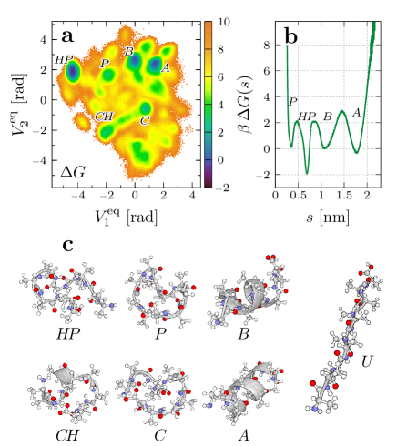
Figure 1: Unbiased MD simulation of Ala₁₀. (a) Free energy landscape $\Delta G(V_{1}^{\rm eq},V_{2}^{\rm eq})$ (in units of $k_{\mathrm{B}}T$) along the first two principal components obtained from dPCA+. (b) Free energy profile $\Delta G(s)$ with respect to the pulling coordinate. (c) Molecular structures of the main metastable conformational states.

Projecting the unbiased data onto pulling coordinate $s$ (which here represents an unconstrained stochastic variable), the free energy profile $\Delta G(s)$ only reveals the main conformational states HP, $A$, $B$ and $P$ (Fig. 1b). In particular, we note that the connectivity is not preserved in the one-dimensional representation, since state HP (instead of $P$) is now direct neighbor of state $B$. In fact, when we plot the free energy as a function of $s$ and $V_{1}^{\rm eq}$ or $V_{2}^{\rm eq}$ (Fig. S2), we find that for $s\lesssim 1$ nm several conformational states may coexist for the same value of $s$. As a consequence, the time evolution of $s(t)$ exhibits jumps between $s\approx$ 0.4 and 1.1 nm (Fig. S2), reflecting that the system directly transits from $P$ to $B$ (as suggested by Fig. 1a). Hence for $s\lesssim 1$ nm the pulling coordinate $s$ represents a poor choice of a reaction coordinate.

III.2 Comparison of unbiased and constrained simulations

The discussion above indicates that TMD simulations are difficult to interpret for $s\lesssim 1$ nm, since several free energy minima may occur for the same value of pulling coordinate $s$. On the other hand, we noticed that the sampling of the unbiased simulation is restricted to $s\!\lesssim\!2$ nm (Fig. 1b), although TMD simulations may be extended to study the unfolding of Ala₁₀ ($s\!\approx\!3$ nm, see below). To achieve a meaningful comparison of MD and TMD simulations, in the following we therefore restrict ourselves to the range of 1.1 nm$\,\leq s\leq\,$2.1 nm, which enables us to describe transitions between states $B$ and $A$. In particular, the comparison allows us to validate the theory developed above.

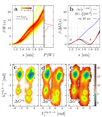
Figure 2: Comparison of unbiased MD and nonequilibrium TMD simulations for the interval 1.1 nm$\,\leq s\leq\,$2.1 nm, describing transitions between states $B$ and $A$ of Ala₁₀. (a) Distribution of work performed on the system by external pulling along coordinate $s$. On the right, the cut $P(W)$ at $s=1.77$ nm reveals non-Gaussian structure. (b) Comparison of free energy profiles $\Delta G(s)$ obtained from unbiased MD simulation (black), Jarzynski’s identity (red), and second-order cumulant approximation (blue). (c-e) Energy landscapes (in units of $k_{\mathrm{B}}T$) as a function of the first two principal components obtained from dPCA+ performed for 1.1 nm$\,\leq s\leq\,$2.1 nm. Compared are (c) results from unbiased MD, (d) TMD, and (e) reweighted TMD.

In order to characterize the nonequilibrium simulations, we recall that $\Delta G=\left<W\right>-W_{\rm diss}$, stating that the free energy difference results from the work performed on the system minus the dissipated energy. To begin with the performed work, Fig. 2a shows that the work distribution reveals a complicated structure, including two prominent maxima and several smaller contributions due to rare and wide-spread trajectories. The associated free energy profile $\Delta G(s)$ obtained from Jarzynski’s identity (Fig. 2b) shows two minima reflecting states $B$ and $A$. This result agrees well with the outcome of the unbiased simulations, while the second-order cumulant approximation [Eq. (26)] fails to reproduce $\Delta G(s)$ due to the non-Gaussian structure of the work distribution. Owing to the complicated structure of the work distribution, we needed to run $10\,000$ short nonequilibrium trajectories to achieve satisfactory agreement of TMD and unbiased simulations (see Fig. S3a,b for a study of the convergence behavior). This is a consequence of the exponential average, $\mathrm{e}^{-\beta\Delta G(s)}=\left\langle e^{-\beta W(s)}\right\rangle_{\rm neq}$, where mainly rare low-$W$ trajectories dominate the free energy estimate. Since $\Delta G(s)$ is considerably lower than the average work $\langle W(s)\rangle$, the stretching of state $B$ into helix $A$ with velocity $v_{\rm c}=1$ m/s generates considerable irreversible heat via intramolecular friction.Cellmer08 ; Schulz12 ; Soranno12 ; Erbas13 ; Echeverria14

Having verified that the TMD simulations correctly reproduce the free energy profile $\Delta G(s)$, we are in a position to consider to what extent TMD allows us to predict the free energy along a general reaction coordinate ${\boldsymbol{x}}$. As suitable coordinates we choose the first two principal components $V_{1}^{\text{eq},\scriptscriptstyle{B\shortrightarrow A}}$ and $V_{2}^{\text{eq},\scriptscriptstyle{B\shortrightarrow A}}$ obtained from dPCA+, which was performed for all unbiased trajectory points that lie in the interval 1.1 nm$\,\leq s\leq\,$2.1 nm. Figure 2c shows the resulting free energy landscape obtained from unbiased MD data. Compared to the energy landscape pertaining to the complete data set (Fig. 1a), we note that only the adjacent minima of $B$ and $A$ are included, since all other states are associated with values of $s\leq 1.1\,$nm. The two-dimensional representation $\Delta G(V_{1}^{\text{eq},\scriptscriptstyle{B\shortrightarrow A}},V_{2}^{\text{eq},\scriptscriptstyle{B\shortrightarrow A}})$ can be employed to explain the prominent features of the work distribution (Fig. 2a) in terms of pathways on the free energy surface. Roughly speaking, high-$W$ trajectories mostly transfer directly between states $B$ and $A$, while low-$W$ trajectories typically do not reach state $A$ at $s=2.1\,$nm, since several populated regions coexist for this value of $s$ (Fig. S4). We note that in general there is no direct correspondence between routes in work space and paths in real space.

Using the same coordinates, Fig. 2d shows the energy landscape associated with the nonequilibrium distribution generated by the TMD simulations [Eq. (15)]. Overall, nonequilibrium results and unbiased results (Fig. 2c) appear quite similar, because the free energy $\Delta G(s)$ (and thus the weighting $P(s)$) pertaining to states $B$ and $A$ is alike. In detail, however, the nonequilibrium energy landscape shows a population shift from state $A$ to some side minima at lower values of $V_{2}^{\text{eq},\scriptscriptstyle{B\shortrightarrow A}}$. Moreover, the TMD simulations affect a sampling of high-energy regions (shown in orange), that are not accessible to the unbiased simulation. Lastly, Fig. 2e shows the energy landscape associated with the reweighted nonequilibrium data [Eq. (11)]. As expected, this energy landscape is indeed quite similar to the unbiased equilibrium result in Fig. 2c. Considering the high amount of dissipated work, this similarity appears quite remarkable.

To compare equilibrium, nonequilibrium, and reweighted nonequilibrium data (Figs. 2c-e), we have so far employed principal components generated from unbiased equilibrium MD. Alternatively, these data may be also examined using principal components generated from nonequilibrium data, see Eq. (22). Owing to the similar weighting $P(s)$ of states $B$ and $A$, the resulting energy landscapes (Fig. S5a) are again quite similar and hardly yield new information. The difference between principal components generated from equilibrium or nonequilibrium data can also be directly studied by comparing the respective covariance matrices. Since the $B\!\rightarrow\!A$ transition mainly involves the folding of the C-terminus residues, TMD simulations that enforce this transition are found to result in enhanced correlations between the last three residues (Fig. S5b). Upon reweighting, the covariance matrix again resumes the structure of the unbiased equilibrium MD.

To summarize, we have shown that the $B\!\rightarrow\!A$ transition of Ala₁₀ can be viewed using principal components generated from equilibrium data [Eq. (19)] or nonequilibrium data [Eq. (22)]. Both representations are well defined as they are simply related via the weighting function $P(s)$. Independent of this choice of representation, we may consider equilibrium, nonequilibrium, or reweighted nonequilibrium data to represent the energy landscapes of the system, see Figs. 2c-e. Due to the similar weighting $P(s)$ of states $B$ and $A$, so far the resulting energy landscapes exhibited only minor differences (but see below).

III.3 TMD simulation of helix unfolding

As a well-established application of pulling simulations, Park03 ; Procacci06 ; Forney08 ; Oberhofer09 ; Hazel14 we consider in Fig. 3 the unfolding of the $\alpha$-helical state of Ala₁₀. Since the free energy difference between helical state $A$ and extended state $U$ is quite large ($\approx 28\,k_{\rm B}T$), this process does virtually not occur in the 20 $\upmu$s long unbiased MD trajectory which only samples up to $s\lesssim 2.2\,$nm. In our TMD simulations, all trajectories start at $s=1.5$ nm in $\alpha$-helical structure $A$, run into a local energy minimum (corresponding to a more favorable helical structure), and successively unfold until they reach the extended state $U$ at $s\approx 3.1$ nm. Unlike the case of the above studied $B\!\rightarrow\!A$ transition, the work distribution of the $A\!\rightarrow\!U$ transition is mono-modal and well approximated by a Gaussian (Fig. 3a). As a consequence, the free energy profile $\Delta G(s)$ obtained from Jarzynski’s identity and of its second-order cumulant approximation [Eq. (26)] are in perfect agreement (Fig. 3b). Moreover, we find that the free energy rapidly converges for already 100 TMD runs (Fig. S3c). This is a consequence of the fact that states $A$ and $U$ are connected by only two well-defined and well-accessible paths that require a minimum number of contact changes (see below).

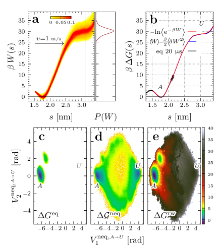
Figure 3: Unfolding of the $\alpha$-helical state $A$ of Ala₁₀. (a) Distribution of work performed on the system by external pulling along coordinate $s$, and a cut $P(W)$ at $s=3.1$ nm. (b) Comparison of free energy profiles $\Delta G(s)$ obtained from unbiased MD simulation (black), Jarzynski’s identity (red), and second-order cumulant approximation (blue). (c-e) Energy landscapes (in units of $k_{\mathrm{B}}T$) as a function of the first two principal components obtained from dPCA+ performed for 1.5 nm$\,\leq s\leq\,$3.5 nm. Compared are (c) results from unbiased equilibrium MD, (d) nonequilibrium TMD, and (e) reweighted TMD.

Due to the large free energy difference of states $A$ and $U$ (and the associated different weighting $P(s)$), we expect large differences when we perform a PCA of unbiased equilibrium and constrained nonequilibrium simulations, respectively. This can be illustrated by the associated covariance matrices which are compared in Fig. 4a. While in the equilibrium case (using all data with $s>1.5$ nm) [Eq. (16)] we find moderate correlations of mostly neighboring residues, virtually all residues are correlated in the nonequilibrium covariance matrix [Eq. (22)]. This is a consequence of the fact that upon unfolding all backbone dihedral angles change from $\alpha$-helical to extended structures. Upon reweighting the nonequilibrium covariances [Eq. (19)], we recover the equilibrium result, as expected.

Let us consider the resulting equilibrium and nonequilibrium principal components $V_{k}^{\text{eq},\scriptscriptstyle{A\shortrightarrow U}}$ and $V_{k}^{\text{neq},\scriptscriptstyle{A\shortrightarrow U}}$, respectively. To elucidate which coordinates are better suited to describe the $A\!\rightarrow\!U$ unfolding process, it is instructive to study the eigenvectors pertaining to the first two components, which account for 50 % (eq) and 90 % (neq) of the total variance, respectively. As shown in Fig. 4b, the eigenvectors of equilibrium components $V_{1}^{\text{eq},\scriptscriptstyle{A\shortrightarrow U}}$ and $V_{2}^{\text{eq},\scriptscriptstyle{A\shortrightarrow U}}$ report exclusively on local motions at the C- and N-terminus, respectively (which is mainly what happens at equilibrium). On the other hand, the eigenvectors of nonequilibrium components $V_{1}^{\text{neq},\scriptscriptstyle{A\shortrightarrow U}}$ and $V_{2}^{\text{neq},\scriptscriptstyle{A\shortrightarrow U}}$ are found to account for the global motion of all residues and thus report directly on the $A\!\rightarrow\!U$ unfolding process.note3 As a further illustration, we plot the energy landscape pertaining to the nonequilibrium data as a function of $s$ and $V_{1}^{\text{eq},\scriptscriptstyle{A\shortrightarrow U}}$ or $V_{1}^{\text{neq},\scriptscriptstyle{A\shortrightarrow U}}$ (Fig. 4c). Since the pulling coordinate evidently corresponds to the direction of maximal variance, we find a direct correlation between $s$ and $V_{1}^{\text{neq},\scriptscriptstyle{A\shortrightarrow U}}$. The second component, on the other hand, is found to split up in two pathways along $s$, thus providing important information beyond the one-dimensional free energy profile $\Delta G(s)$.

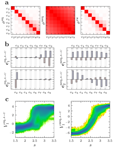
Figure 4: PCA of the $A\!\rightarrow\!U$ unfolding of Ala₁₀. (a) Correlation matrices (i.e., normalized covariances) obtained from (left) unbiased equilibrium MD, (middle) nonequilibrium TMD, and (right) reweighted TMD. (b) Eigenvectors pertaining to the first two principal components, obtained from (left) equilibrium MD and (right) nonequilibrium TMD. (c) Energy landscapes (in units of $k_{\mathrm{B}}T$) as a function of pulling coordinate $s$ and $V_{1}^{\text{eq},A\shortrightarrow U}$ or $V_{1}^{\text{neq},A\shortrightarrow U}$.

We are now in a position to illustrate the $A\!\rightarrow\!U$ unfolding of Ala₁₀ by a multidimensional energy landscape. Using the first two nonequilibrium principal components $V_{k}^{\text{neq},\scriptscriptstyle{A\shortrightarrow U}}$, Fig. 3 shows energy landscapes constructed from (c) unbiased equilibrium MD, (d) nonequilibrium simulations, and (e) reweighted nonequilibrium data. As expected, the unbiased free energy landscape (Fig. 3c) only samples initial state $A$ together with a neighboring state that reflects the breaking of the helix at the N-terminus. The results for the reweighted nonequilibrium data (Fig. 3e) are quite similar, but also show enhanced sampling of high-energy regions. Notably, the energy landscape obtained from the nonequilibrium data (Fig. 3d) is most informative, as it shows the entire conformational space sampled by the TMD simulation including initial state $A$ and final state $U$.

The nonequilibrium energy landscape $\Delta{\cal G}$ [Eq. (15)] indicates two main unfolding pathways, which are discriminated by the second principal component. The upper half circle connecting states $A$ and $U$ reflects trajectories that start unfolding at the N-terminus and continue to the C-terminus, while the lower half circle corresponds to unfolding trajectories proceeding the opposite way. Followed by 75 % of all trajectories, the C$\rightarrow$N path clearly represents the main unfolding route. This may be a consequence of the fact that the C-terminus is able to form hydrogen bonds with both of its oxygen atoms (while the N-terminus can only form a single hydrogen bond), and therefore exhibits larger fluctuations and structural destabilization. Trajectories that initially proceed the opposite N$\rightarrow$C path mostly do not complete this route, but return to the helical state $A$.

To illustrate the C$\rightarrow$N unfolding pathway, Fig. S6a shows the evolution of the peptide’s backbone dihedral angles $\psi_{n}$. As expected, the dihedral angles change sequentially from an $\alpha$-helical ($\psi\approx-40^{\circ}$) to an extended ($\psi\approx 160^{\circ}$) conformation. Using DSSPKabsch83 to characterize the secondary structure of Ala₁₀, however, we find that the helix does not unfold directly, but first changes to a 3₁₀-helix for $s\gtrsim 2$ nm (Fig. S6b). In the course of the unfolding process, the 3₁₀-helix may temporarily turn into a shortened $\alpha$-helix in combination with turn/coil structures. This can occur anywhere in the peptide sequence, thus allowing the helix to break at its weakest end.

As a further characterization of the unfolding mechanism, it is instructive to consider the friction profile ${\it{\Gamma}}(s)$ obtained from dissipation-corrected TMDWolf18 (Fig. S6c). Reflecting the fluctuations of the constraint force [Eq. (27)], ${\it{\Gamma}}(s)$ is not necessarily related to the form of the free energy profile $\Delta G(s)$. As in the previously studied NaCl/water system,Wolf18 the friction profile may therefore provide new microscopic information on the unfolding process. At the onset of unfolding at $s\gtrsim 2.0$ nm, ${\it{\Gamma}}(s)$ starts to increase and comes to a maximum at full extension at $s\approx 2.8$ nm. We attribute this rise in friction to the loose C-terminal chain, which can fluctuate more with increasing length. The sharp minimum of ${\it{\Gamma}}(s)$ at $s\approx 3.0$ nm coincides with a shallow minimum of the $\Delta G(s)$ profile, pointing to a structural relaxation of the chain in the extended conformation. For $s\gtrsim 3.0$ nm the friction increases again, which most likely results from over-stretching the peptide chain.

IV Conclusions

Aiming to describe nonequilibrium phenomena in terms of a multidimensional energy landscape, we have studied the application of dimensionality reduction techniques to nonequilibrium MD data. To be specific, we have focused on principal component analysis (PCA) of targeted MD (TMD) simulationsSchlitter93A ; Schlitter94 ; Schlitter01 that are constrained along some biasing coordinate $s$. We have found that it is generally valid to simply perform PCA on the concatenated nonequilibrium trajectories. While the resulting distribution ${\cal P}({\boldsymbol{x}})$ and energy landscape $\Delta{\cal G}({\boldsymbol{x}})\propto\ln{\cal P}({\boldsymbol{x}})$ will not reflect the equilibrium state of the system, the nonequilibrium energy landscape may directly reveal the molecular reaction mechanism. Applied to the unfolding of the $\alpha$-helical state of Ala₁₀, for example, we have identified two unfolding pathways starting from the C- and N-terminus, respectively. Notably, this information is not available from the commonly calculated free energy profile $\Delta G(s)\propto\ln P(s)$.

The nonequilibrium energy landscape $\Delta{\cal G}({\boldsymbol{x}})$ is well defined, because it is related to the equilibrium free energy landscape through weighting function $P(s)$ accounting for the bias introduced by TMD. That is, by reweighting the TMD conditional probability $P({\boldsymbol{x}}|s)$ by $P(s)$ and subsequently integrating over $s$ [Eq. (8)], we obtain the correct equilibrium distribution $P({\boldsymbol{x}})$. The same holds for PCA, where we construct principal components from nonequilibrium data which are associated to equilibrium principal components constructed from the reweighted data [Eq. (19)]. Although this formulation is in principle exact, its practical use depends on how well the conformational distribution of interest is sampled by nonequilibrium simulations along biasing coordinate $s$. Moreover, it is important that coordinate $s$ accounts for a naturally occurring motion between two well-defined end-states of the system. This is the case for the example of the $A\!\rightarrow\!U$ unfolding reaction of Ala₁₀ (Fig. 3), but less so for the $B\!\rightarrow\!A$ transition (Fig. 2), where the start and end state split up in various metastable states.

While we have focused the discussion on TMD, the above described approach is readily applied to various types of nonequilibrium simulations. In particular, this implies enhanced sampling methods that are described by a continuous and sufficiently slow development along some control parameter $s$ and provide a weighting function $P(s)$, such as umbrella samplingTorrie77 and steered MD,Isralewitz01 ; Park04 conformational flooding,Grubmueller95 metadynamics,Laio02 and adaptive biasing force sampling.Darve08 Moreover, besides PCA alternative dimensionality reduction techniques may be employed including nonlinear techniquesRohrdanz13 ; Duan13 and various kinds of machine learning approaches. Galvelis17 ; Chen18 ; Ribeiro18 ; Brandt18 In ongoing work, we use nonequilibrium PCA to study conformational changes of T4 lysozyme,Ernst17 and to analyze unbinding simulations of small organic molecules from proteins such as the N-terminal domain of Hsp90Amaral17 and the $\beta_{2}$ adrenergic receptor.Cherezov07

Supplementary Material

Details of dPCA+, energy landscapes as a function of $s$ and various principal components, evolution of pulling coordinate, dihedral angles, secondary structure content and friction content, convergence tests of free energy estimators.

Acknowledgment

We thank Simon Bray for instructive and helpful discussions. This work has been supported by the Deutsche Forschungsgemeinschaft (Sto 247/11) and the bwUniCluster computing initiatives of the State of Baden-Württemberg. We furthermore acknowledge support by the High Performance and Cloud Computing Group at the Zentrum für Datenverarbeitung of the University of Tübingen, the state of Baden-Württemberg through bwHPC, and the Deutsche Forschungsgemeinschaft through grant no. INST 37/935-1 FUGG.

The dPCA+ methodSittel17 was implemented in the open source software FastPCA. Dissipation-corrected TMDWolf18 was implemented using Python3. All programs are freely available at https://github.com/moldyn.

References

- (1) J. N. Onuchic, Z. L. Schulten, and P. G. Wolynes, Theory of protein folding: The energy landscape perspective, Annu. Rev. Phys. Chem. 48, 545 (1997).
- (2) K. A. Dill and H. S. Chan, From Levinthal to pathways to funnels: The ”new view” of protein folding kinetics, Nat. Struct. Bio. 4, 10 (1997).
- (3) D. J. Wales, Energy Landscapes, Cambridge University Press, Cambridge, 2003.
- (4) M. A. Rohrdanz, W. Zheng, and C. Clementi, Discovering mountain passes via torchlight: Methods for the definition of reaction coordinates and pathways in complex macromolecular reactions, Annu. Rev. Phys. Chem. 64, 295 (2013).
- (5) B. Peters, Reaction coordinates and mechanistic hypothesis tests, Annu. Rev. Phys. Chem. 67, 669 (2016).
- (6) F. Noe and C. Clementi, Collective variables for the study of long-time kinetics from molecular trajectories: theory and methods, Curr. Opin. Struct. Biol. 43, 141 (2017).
- (7) F. Sittel and G. Stock, Perspective: Identification of collective coordinates and metastable states of protein dynamics, J. Chem. Phys. 149, 150901 (2018).
- (8) A. Amadei, A. B. M. Linssen, and H. J. C. Berendsen, Essential dynamics of proteins, Proteins 17, 412 (1993).
- (9) Y. Mu, P. H. Nguyen, and G. Stock, Energy landscape of a small peptide revealed by dihedral angle principal component analysis, Proteins 58, 45 (2005).
- (10) C. Chipot and A. Pohorille, Free Energy Calculations, Springer, Berlin, 2007.
- (11) C. D. Christ, A. E. Mark, and W. F. van Gunsteren, Basic Ingredients of Free Energy Calculations: A Review, J. Comput. Chem. 31, 1569 (2010).
- (12) G. Fiorin, M. L. Klein, and J. Henin, Using collective variables to drive molecular dynamics simulations, Mol. Phys. 111, 3345 (2013).
- (13) G. A. Tribello, M. Bonomi, D. Branduardi, C. Camilloni, and G. Bussi, PLUMED 2: New feathers for an old bird, Comp. Phys. Comm. 185, 604 (2014).
- (14) Y. Sugita and Y. Okamoto, Replica-exchange molecular dynamics method for protein folding, Chem. Phys. Lett. 314, 141 (1999).
- (15) H. Grubmüller, Predicting slow structural transitions in macromolecular systems: Conformational flooding, Phys. Rev. E 52, 2893 (1995).
- (16) F. Rico, A. Russek, L. González, H. Grubmüller, and S. Scheuring, Heterogeneous and rate-dependent streptavidin–biotin unbinding revealed by high-speed force spectroscopy and atomistic simulations, Proc. Natl. Acad. Sci. USA 116, 6594 (2019).
- (17) A. Laio and M. Parrinello, Escaping free-energy minima, Proc. Natl. Acad. Sci. USA 99, 12562 (2002).
- (18) E. Darve, D. Rodriguez-Gomez, and A. Pohorille, Adaptive biasing force method for scalar and vector free energy calculations, J. Chem. Phys. 128, 144120 (2008).
- (19) G. M. Torrie and J. P. Valleau, Non-physical sampling distributions in Monte-Carlo free-energy estimation - umbrella sampling, J. Comput. Phys. 23, 187 (1977).
- (20) B. Isralewitz, M. Gao, and K. Schulten, Steered molecular dynamics and mechanical functions of proteins, Curr. Opin. Struct. Biol. 11, 224 (2001).
- (21) S. Park and K. Schulten, Calculating potentials of mean force from steered molecular dynamics simulations, J. Chem. Phys. 120, 5946 (2004).
- (22) M. Sprik and G. Ciccotti, Free energy from constrained molecular dynamics, J. Chem. Phys. 109, 7737 (1998).
- (23) G. Ciccotti, R. Kapral, and E. Vanden-Eijnden, Blue moon sampling, vectorial reaction coordinates, and unbiased constrained dynamics, ChemPhysChem 6, 1809 (2005).
- (24) J. Schlitter, M. Engels, P. Krüger, E. Jacoby, and A. Wollmer, Targeted Molecular Dynamics Simulation of Conformational Change-Application to the T R Transition in Insulin, Mol. Simul. 10, 291 (1993).
- (25) J. Schlitter, M. Engels, and P. Krüger, Targeted molecular dynamics - a new approach for searching pathways of conformational transitions, J. Mol. Graph. 12, 84 (1994).
- (26) J. Schlitter, W. Swegat, and T. Mülders, Distance-type reaction coordinates for modelling activated processes, J. Mol. Model. 7, 171 (2001).
- (27) In the original paper by Schlitter et al.,Schlitter93A TMD comprises both a directionality and a dynamical aspect. Regarding directionality, TMD propagates a molecular system along a pre-chosen reaction coordinate towards a target state (e.g., a specific conformational state of the system). The propagation (i.e., the dynamical aspect) is achieved by applying a holonomic constraint via Lagrange multipliers. In this sense, TMD is closely related to the constrained MD method by Cicotti et al.Sprik98 ; Ciccotti05 as well as to the essential dynamics method by Amadei et al.Amadei96 .
- (28) H. J. C. Berendsen, Simulating the Physical World, Cambridge University Press, Cambridge, 2007.
- (29) C. Jarzynski, Nonequilibrium equality for free energy differences, Phys. Rev. Lett. 78, 2690 (1997).
- (30) T. Mülders, P. Krüger, W. Swegat, and J. Schlitter, Free energy as the potential of mean constraint force, J. Chem. Phys. 104, 4869 (1996).
- (31) S. Kumar, J. Rosenberg, D. Bouzida, R. Swendsen, and P. Kollman, The weighted histogram analysis method for free-energy calculations on biomolecules. I. The method, J. Comput. Chem. 13, 1011 (1992).
- (32) G. Hummer and A. Szabo, Free energy reconstruction from nonequilibrium single-molecule pulling experiments, Proc. Natl. Acad. Sci. USA 98, 3658 (2001).
- (33) G. Hummer and A. Szabo, Free energy surfaces from single-molecule force spectroscopy, Acc. Chem. Res. 38, 504 (2005).
- (34) D. A. Hendrix and C. Jarzynski, A “fast growth” method of computing free energy differences, J. Chem. Phys. 114, 5974 (2001).
- (35) H. Oberhofer and C. Dellago, Efficient extraction of free energy profiles from nonequilibrium experiments, J. Comput. Chem. 30, 1726 (2009).
- (36) C. Dellago and G. Hummer, Computing equilibrium free energies using non-equilibrium molecular dynamics, Entropy 16, 41 (2014).
- (37) S. Wolf and G. Stock, Targeted molecular dynamics calculations of free energy profiles using a nonequilibrium friction correction, J. Chem. Theory Comput. 14, 6175 (2018).
- (38) S. Park, F. Khalili-Araghi, E. Tajkhorshid, and K. Schulten, Free energy calculation from steered molecular dynamics simulations using Jarzynski’s equality, J. Chem. Phys. 119, 3559 (2003).
- (39) P. Procacci, S. Marsili, A. Barducci, G. F. Signorini, and R. Chelli, Crooks equation for steered molecular dynamics using a Nosé-Hoover thermostat, J. Chem. Phys. 125, 164101 (2006).
- (40) M. W. Forney, L. Janosi, and I. Kosztin, Calculating free-energy profiles in biomolecular systems from fast nonequilibrium processes, Phys. Rev. E 78, 051913 (2008).
- (41) A. Hazel, C. Chipot, and J. C. Gumbart, Thermodynamics of Deca-alanine Folding in Water, J. Chem. Theory Comput. 10, 2836 (2014).
- (42) We note in passing that in general the change from free to constrained motion involves the inclusion of the so-called Fixman potential, Fixman74 associated with the integration over the conjugated momentum of constrained coordinate . Choosing to be a linear combination of interatomic distances (as is usually done in TMD), however, this determinant reduces to a constant Schlitter01 .
- (43) G. E. Crooks, Path-ensemble averages in systems driven far from equilibrium, Phys. Rev. E 61, 2361 (2000).
- (44) J. M. R. Parrondo, J. M. Horowitz, and T. Sagawa, Thermodynamics of information, Nat. Phys. 11, 131 (2015).
- (45) A. Altis, M. Otten, P. H. Nguyen, R. Hegger, and G. Stock, Construction of the free energy landscape of biomolecules via dihedral angle principal component analysis, J. Chem. Phys. 128, 245102 (2008).
- (46) Note that is the deviation of restricted by a fixed from its equilibrium mean (not the average at ), which for TMD simulations can be readily calculated via Eq. (II.1).
- (47) M. J. Abraham, T. Murtola, R. Schulz, S. Páll, J. C. Smith, B. Hess, and E. Lindahl, Gromacs: High performance molecular simulations through multi-level parallelism from laptops to supercomputers, SoftwareX 1–2, 19 (2015).
- (48) J. Huang and A. D. MacKerell, Charmm36 all-atom additive protein force field: Validation based on comparison to NMR data, J. Comput. Chem. 34, 2135 (2013).
- (49) G. Bussi, D. Donadio, and M. Parrinello, Canonical sampling through velocity rescaling, J. Chem. Phys. 126, 0141011 (2007).
- (50) B. Hess, P-lincs: A parallel linear constraint solver for molecular simulation, J. Chem. Theory Comput. 4, 116 (2008), PMID: 26619985.
- (51) T. Darden, D. York, and L. Petersen, Particle mesh Ewald: An N log(N) method for Ewald sums in large systems, J. Chem. Phys. 98, 10089 (1993).
- (52) W. Humphrey, A. Dalke, and K. Schulten, VMD – Visual Molecular Dynamics, J. Mol. Graph. 14, 33 (1996).
- (53) Schrödinger, LLC, The PyMOL molecular graphics system, version 1.8, (2015).
- (54) J. P. Ryckaert, G. Ciccotti, and H. J. C. Berendsen, Numerical-integration of cartesian equations of motions of a system with constraints-molecular dynamics of n-alkanes, J. Comput. Phys. 23, 327 (1977).
- (55) M. Ernst, F. Sittel, and G. Stock, Contact- and distance-based principal component analysis of protein dynamics, J. Chem. Phys. 143, 244114 (2015).
- (56) F. Sittel, A. Jain, and G. Stock, Principal component analysis of molecular dynamics: On the use of Cartesian vs. internal coordinates, J. Chem. Phys. 141, 014111 (2014).
- (57) A. Altis, P. H. Nguyen, R. Hegger, and G. Stock, Dihedral angle principal component analysis of molecular dynamics simulations, J. Chem. Phys. 126, 244111 (2007).
- (58) F. Sittel, T. Filk, and G. Stock, Principal component analysis on a torus: Theory and application to protein dynamics, J. Chem. Phys. 147, 244101 (2017).
- (59) T. Cellmer, E. R. Henry, J. Hofrichter, and W. A. Eaton, Measuring internal friction of an ultrafast-folding protein, Proc. Natl. Acad. Sci. USA 105, 18320 (2008).
- (60) J. C. F. Schulz, L. Schmidt, R. B. Best, J. Dzubiella, and R. R. Netz, Peptide chain dynamics in light and heavy water: Zooming in on internal friction, J. Am. Chem. Soc. 134, 6273 (2012).
- (61) A. Soranno, B. Buchli, D. Nettels, R. R. Cheng, S. Müller-Späth, S. H. Pfeil, A. Hoffmann, E. A. Lipman, D. E. Makarov, and B. Schuler, Quantifying internal friction in unfolded and intrinsically disordered proteins with single-molecule spectroscopy, Proc. Natl. Acad. Sci. USA 109, 17800 (2012).
- (62) A. Erbaş and R. R. Netz, Confinement-Dependent Friction in Peptide Bundles, Biophys. J. 104, 1285 (2013).
- (63) I. Echeverria, D. E. Makarov, and G. A. Papoian, Concerted dihedral rotations give rise to internal friction in unfolded proteins, J. Am. Chem. Soc. 136, 8708 (2014).
- (64) In fact, the overall structure of eigenvectors and corresponds to the typical shape of the first two normal modes of a harmonic chain.
- (65) W. Kabsch and C. Sander, Dictionary of protein secondary structure: Pattern recognition of hydrogen bonded and geometrical features, Biopolymers 22, 2577 (1983).
- (66) M. Duan, J. Fan, M. Li, L. Han, and S. Huo, Evaluation of dimensionality-reduction methods from peptide folding-unfolding simulations, J. Chem. Theory Comput. 9, 2490 (2013).
- (67) R. Galvelis and Y. Sugita, Neural network and nearest neighbor algorithms for enhancing sampling of molecular dynamics, J. Chem. Theory Comput. 13, 2489 (2017).
- (68) W. Chen, A. R. Tan, and A. L. Ferguson, Collective variable discovery and enhanced sampling using autoencoders: Innovations in network architecture and error function design, J. Chem. Phys. 149, 072312 (2018).
- (69) J. M. L. Ribeiro, P. Bravo, Y. Wang, and P. Tiwary, Reweighted autoencoded variational bayes for enhanced sampling (rave), J. Chem. Phys. 149, 072301 (2018).
- (70) S. Brandt, F. Sittel, M. Ernst, and G. Stock, Machine learning of biomolecular reaction coordinates, J. Phys. Chem. Lett. 9, 2144 (2018).
- (71) M. Ernst, S. Wolf, and G. Stock, Identification and validation of reaction coordinates describing protein functional motion: Hierarchical dynamics of T4 Lysozyme, J. Chem. Theory Comput. 13, 5076 (2017).
- (72) M. Amaral, D. B. Kokh, J. Bomke, A. Wegener, H. P. Buchstaller, H. M. Eggenweiler, P. Matias, C. Sirrenberg, R. C. Wade, and M. Frech, Protein conformational flexibility modulates kinetics and thermodynamics of drug binding., Nat. Commun. 8, 2276 (2017).
- (73) V. Cherezov et al., High-Resolution Crystal Structure of an Engineered Human 2-Adrenergic G Protein Coupled Receptor, Science 318, 1258 (2007).
- (74) A. Amadei, A. B. M. Linssen, B. L. de Groot, D. M. F. van Aalten, and H. J. C. Berendsen, An Efficient Method for Sampling the Essential Subspace of Proteins, J. Biomol. Struct. Dyn. 13, 615 (1996).
- (75) M. Fixman, Classical statistical mechanics of constraints: A theorem and application to polymers, Proc. Natl. Acad. Sci. USA 71, 3050 (1974).