Simple non-perturbative resummation schemes beyond mean-field II: thermodynamics of scalar $\phi^{4}$ theory in 1+1 dimensions at arbitrary coupling

Abstract

Recently, non-perturbative approximate solutions were presented that go beyond the well-known mean-field resummation. In this work, these non-perturbative approximations are used to calculate finite temperature equilibrium properties for scalar $\phi^{4}$ theory in two dimensions such as the pressure, entropy density and speed of sound. Unlike traditional approaches, it is found that results are well-behaved for arbitrary temperature/coupling strength, are independent of the choice of the renormalization scale $\bar{\mu}^{2}$, and are apparently converging as the resummation level is increased. Results also suggest the presence of a possible analytic cross-over from the high-temperature to the low-temperature regime based on the change in the thermal entropy density.

I Introduction

Recently, I presented a sequence of non-perturbative approximate solutions for scalar $\phi^{4}$ theory for arbitrary interaction strength Romatschke (2019). These approximate solutions contain, but allow to systematically improve on, the familiar mean-field approximation. In this work, I consider $\phi^{4}$ field theory in two dimensions at finite temperature as a natural extension of the zero-temperature study done in Ref. Romatschke (2019).

Finite temperature quantum field theory is a mature and well-established discipline Laine and Vuorinen (2016). At high temperature, naive perturbation theory breaks down because of infrared singularities. These difficulties are by now understood to be cured by resumming an infinite number of Feynman diagrams, generating an effective in-medium (thermal) mass. This “Hard-Thermal-Loop” (HTL) resummation Braaten and Pisarski (1990a) has led to a very successful program for calculating properties of field theories at finite temperature and/or density, cf. Refs. Taylor and Wong (1990); Braaten and Pisarski (1990b, 1992); Braaten and Yuan (1991); Kelly et al. (1994); Flechsig and Rebhan (1996); Moore et al. (1998); Carrington et al. (1999); Andersen et al. (1999); Bodeker et al. (2000); Blaizot et al. (1999); Bolz et al. (2001); Karsch et al. (2001); Peshier (2001); Blaizot et al. (2001a, b); Blaizot and Iancu (2002); Rebhan and Romatschke (2003); Romatschke and Strickland (2003); Kraemmer and Rebhan (2004); Andersen and Strickland (2005); Rebhan et al. (2005); Laine et al. (2007); Caron-Huot and Moore (2008); Rychkov and Strumia (2007); Ghiglieri et al. (2013); Haque et al. (2014); Gorda et al. (2018).

So why invest time into developing novel resummation schemes, given the apparent success of the HTL resummation program?

First, despite resumming an infinite number of Feynman diagrams, the HTL resummation scheme is not fully non-perturbative in the sense that HTL results do not exhibit a sensible strong-coupling limit. Second, the HTL resummation scheme does not easily incorporate the physics of transport which typically requires resummation of higher-order Feynman diagrams. Third, observables exhibit an unphysical dependence on the renormalization scale choice, which is a property inherited from perturbative truncations of the full theory.

This provides the motivation to consider the resummation schemes R0-R3 described in Ref. Romatschke (2019) to test if any of these issues arsing for the HTL resummation scheme can be improved on. For simplicity of presentation, I chose to ignore transport properties for the present work and only study equilibrium thermodynamics.

II Finite temperature pressure of scalar $\phi^{4}$ theory in 2d

Let me consider the path integral formulation of $\phi^{4}$ theory in two Euclidean dimensions given by

$$Z=\int{\cal D}\phi e^{-S}\,,\quad S=\int d^{2}X\left(\frac{1}{2}\partial_{\mu}\phi\partial_{\mu}\phi+\frac{m^{2}}{2}\phi^{2}+\lambda\phi^{4}\right)\,,\quad X=\left(\tau,x\right)\,,$$ (1)

where $\lambda$ has mass dimension two and $m^{2}>0$ is assumed. The Euclidean time direction $\tau$ is compactified on a circle with radius $\beta\equiv T^{-1}$, where $T$ is the equilibrium temperature of the system. Introducing an auxiliary field $\zeta$, the path integral may be re-written as

$$Z=\sqrt{\frac{\beta V}{16\lambda\pi}}\int d\zeta_{0}e^{-\frac{\zeta_{0}^{2}\beta V}{16\lambda}}\int{\cal D}\phi{\cal D}\zeta^{\prime}e^{-S_{0}-S_{I}}\,,$$ (2)

where $V$ is the “volume” of the Euclidean direction $x$ and

$$S_{0}=\frac{1}{2}\int d^{2}X\left[\partial_{\mu}\phi\partial_{\mu}\phi+m^{2}\phi^{2}+i\zeta_{0}\phi^{2}+\frac{\zeta^{\prime 2}}{2\lambda}\right]\,,\quad S_{I}=i\int d^{2}X\zeta^{\prime}\phi^{2}\,,$$ (3)

and $\zeta_{0}$ is the global zero mode of $\zeta$. The resummation schemes R0-R3 introduced in Ref. Romatschke (2019) correspond to different approximation levels (R0 the “coarsest” and R3 the “finest”) of the partition function.

II.1 R0-level

In the R0 scheme, the term $S_{I}$ is dropped completely, and the partition function may be evaluated analytically as Romatschke (2019)

$$Z_{R0}=\sqrt{\frac{\beta V}{16\lambda\pi}}\int d\zeta_{0}e^{-\beta V\left[\frac{\zeta_{0}^{2}}{16\lambda}+J\left(\sqrt{m^{2}+i\zeta_{0}}\right)\right]}\,,$$ (4)

where $J(\alpha)=J_{0}(\alpha)+J_{T}(\alpha)$ and in $d=1-2\epsilon$ Euclidean space dimensions Laine and Vuorinen (2016)

$$J_{0}(\alpha)=\frac{\alpha^{2}}{8\pi\epsilon}+\frac{\alpha^{2}}{8\pi}\ln\frac{\bar{\mu}^{2}e^{1}}{\alpha^{2}}+{\cal O}(\epsilon)\,,\quad J_{T}(\alpha)=-\frac{\alpha T}{\pi}\sum_{n=1}^{\infty}\frac{K_{1}\left(\frac{n\alpha}{T}\right)}{n}+{\cal O}(\epsilon)\,.$$ (5)

Here $\bar{\mu}^{2}=4\pi\mu^{2}e^{-\gamma_{E}}$ is the $\overline{\rm MS}$ scale parameter that in finite-temperature field theory literature is customarily varied by a factor two around the first non-vanishing Matsubara frequency, e.g. $\bar{\mu}\in\left[\pi T,4\pi T\right]$. Physical observables are not meant to depend on $\bar{\mu}$, hence varying $\bar{\mu}$ in truncations of the full theory is used to test for the sensitivity of results to higher-order terms not considered in the approximation.

In the large volume limit $V\rightarrow\infty$, the partition function in the R0 approximation may be evaluated through a saddle-point approximation, finding

$$Z_{R0}=e^{-\beta V\left[-\frac{z^{*2}_{R0}}{16\lambda}+J\left(\sqrt{m^{2}+z_{R0}^{*}}\right)\right]}\,,\quad i\zeta_{0}=z^{*}_{R0}=4\lambda I\left(\sqrt{m^{2}+z_{R0}^{*}}\right)\,,$$ (6)

where $I(\alpha)=2\frac{dJ(\alpha)}{d\alpha^{2}}$. At zero temperature, the theory is renormalized by requiring a finite pole mass of the two-point function $\langle\phi(x)\phi(0\rangle$, which in the R0 approximation leads to $m^{2}_{R}=m^{2}+\frac{\lambda}{\pi\epsilon}$ Romatschke (2019). Solving the resulting renormalization group equation hence gives the running of the renormalized mass $m_{R}^{2}$ with the renormalization scale $\bar{\mu}^{2}$ as

$$m_{R}^{2}\left(\bar{\mu}^{2}\right)=m_{F}^{2}-\frac{\lambda}{\pi}\ln\frac{\bar{\mu}^{2}}{m_{F}^{2}}\,,$$ (7)

where $m_{F}^{2}$ is the value of the renormalized mass at some fiducial scale. Given that $\lambda$ has mass dimension two, it is useful to consider units in which all other dimensionful quantities are expressed in terms of $\lambda$, e.g.

$$\hat{m}_{R}^{2}\equiv\frac{m_{R}^{2}}{\lambda}\,,\quad\hat{T}\equiv\frac{T}{\sqrt{\lambda}},\quad\hat{\mu}^{2}=\frac{\bar{\mu}^{2}}{\lambda}\,.$$ (8)

Note that in these units, the weak-coupling regime corresponds to high temperature $\hat{T}\rightarrow\infty$, whereas low temperature corresponds to strong coupling, similar to studies of dimensionally reduced gauge theories and gauge/gravity duality Aharony et al. (2004); Kawahara et al. (2007); Hanada and Romatschke (2017). For simplicity of notation, I will drop the hat notation in the following, effectively using units where $\lambda=1$.

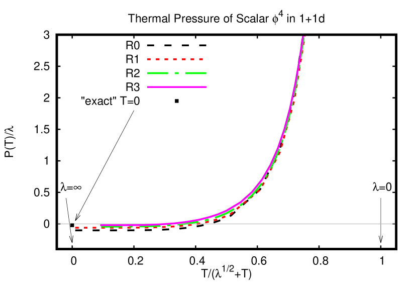
Figure 1: Thermal pressure as a function of re-scaled temperature $T/\sqrt{\lambda}$ for $m_{F}^{2}=\lambda$ in the R0-R3 approximation scheme. Results do not depend on the renormalization scale choice $\bar{\mu}$. Horizontal plot axis is expressed as $\frac{T}{T+\sqrt{\lambda}}$ to allow compactification of the whole interval $T\in[0,\infty)$. Arrows indicate location of weak and strong coupling regime $\lambda=0$, $\lambda=\infty$, respectively, as well as the location of the zero-temperature result from high precision (“exact”) calculations (34) using Refs. Serone et al. (2018); Elias-Miro et al. (2017). Full line is a guide to the eye.

The partition function can be written as

$$Z=e^{\beta V\left(P(T,\bar{\mu}^{2})+P_{\rm div}\right)}\,,$$ (9)

where $P_{\rm div}=\frac{m^{4}}{16}$ is a divergent contribution to the cosmological constant in the R0-level approximation and the finite-temperature pressure is given by

$$P_{R0}(T,\bar{\mu}^{2})=-J_{T}(M)+\frac{M^{4}}{16}-\frac{M^{2}m_{R}^{2}}{8}-\frac{M^{2}}{8\pi}\ln\frac{\bar{\mu}^{2}e^{1}}{M^{2}}\,,$$ (10)

with a self-consistent pole mass $M$ determined by the solution of the “gap” equation

$$M^{2}=m^{2}+z_{R0}^{*}=m_{R}^{2}+\frac{1}{\pi}\ln\frac{\bar{\mu}^{2}}{M^{2}}+4I_{T}(M)=m_{F}^{2}+\frac{1}{\pi}\ln\frac{m_{F}^{2}}{M^{2}}+4I_{T}(M)\,.$$ (11)

Using the running of $m_{R}^{2}$ in the R0-level approximation (7), one may verify explicitly that the finite-temperature pressure $P_{R0}(T,\bar{\mu}^{2})$ is independent from the choice of the renormalization scale $\bar{\mu}^{2}$. At very high temperature, the R0-pressure reduces to the pressure of a free scalar field in two dimensions,

$$P_{free}=\frac{\pi T^{2}}{6}\,,$$ (12)

as expected for a weakly coupled field theory. At finite temperature, the R0 level approximation results in a reduction of the pressure from the free result, which contains all orders in perturbation theory partially through the self-consistent solution of the gap equation (11). At zero temperature, the $P_{R0}(T=0)=-\frac{m_{F}^{4}}{16}-\frac{m_{F}^{2}}{8\pi}$ contains a finite contribution to the cosmological constant. A plot of the pressure for the R0 approximation is shown in Fig. 1 for $m_{F}^{2}=1$. While only part of the temperature range is visible in this figure, the pressure is well-behaved for all temperatures, and smoothly interpolates from the weak-coupling, high-temperature regime to the strong-coupling, low temperature regime.

II.2 R1-level

Without further input, it is not clear how good an approximation the R0-level resummation for the true finite-temperature pressure of scalar $\phi^{4}$ really is. A step forward can be made by considering the next best approximation level, R1, which arises from (2) by a suitable re-shuffling of terms between $S_{0},S_{I}$ (see Ref. Romatschke (2019) for details), finding

$$Z_{R1}=\sqrt{\frac{\beta V}{16\pi}}\int d\zeta_{0}e^{-\beta V\left[\frac{\zeta_{0}^{2}}{16}+J\left(\sqrt{m^{2}+3i\zeta_{0}}\right)-2I^{2}\left(\sqrt{m^{2}+3i\zeta_{0}}\right)\right]}\,.$$ (13)

In the large volume limit, the partition function can once again be evaluated through a saddle point approximation, finding $i\zeta_{0}=z_{R1}^{*}=4I\left(\sqrt{m^{2}+3z_{R1}^{*}}\right)$. The zero-temperature pole mass is rendered finite by introducing a renormalized mass squared $m_{R}^{2}=m^{2}+\frac{3}{\pi\epsilon}$ Romatschke (2019), which leads to the mass running as

$$m_{R}^{2}\left(\bar{\mu}^{2}\right)=m_{F}^{2}-\frac{3}{\pi}\ln\frac{\bar{\mu}^{2}}{m_{F}^{2}}\,,$$ (14)

cf. the corresponding equation (7) in the R0-level approximation. The partition function can once again be written in the form (9) with a divergent contribution $P_{\rm div}=\frac{m^{4}}{48}$ and a finite-temperature pressure

$$P_{R1}(T,\bar{\mu}^{2})=-J_{T}(M)+\frac{M^{4}}{48}-\frac{M^{2}m_{R}^{2}}{24}-\frac{M^{2}}{8\pi}\ln\frac{\bar{\mu}^{2}e^{1}}{M^{2}}\,.$$ (15)

Here $M^{2}$ is the self-consistent pole mass determined as the solution of the gap equation

$$M^{2}=m^{2}+3z_{R1}^{*}=m_{R}^{2}+\frac{3}{\pi}\ln\frac{\bar{\mu}^{2}}{M^{2}}+12I_{T}(M)=m_{F}^{2}+\frac{3}{\pi}\ln\frac{m_{F}^{2}}{M^{2}}+12I_{T}(M)\,.$$ (16)

Similar to what was found for the R0-level approximation, the running $m_{R}^{2}$ ensures that the R1-level pressure (15) is independent from the choice of the renormalization scale $\bar{\mu}^{2}$. (This is somewhat trivial for a super-renormalizable theory such as $\phi^{4}$ in 1+1 dimensions. However, the behavior persists for theories that are just renormalizable, as has been explicitly shown in Ref. Blaizot et al. (2001a) corresponding to the R1 scheme for $\phi^{4}$ theory in 3+1 dimensions). Results for $P_{R1}(T)$ are shown in Fig. 1 as a function of temperature. While the leading perturbative correction term to $P_{free}$ originating from $P_{R0}(T)$ is only a third of that from $P_{R1}(T)$, Fig. 1 shows that R0 and R1-level approximations give similar results for the overall pressure magnitude for all values of temperatures/couplings shown. (There are notable relative differences for low temperatures, given that $P_{R1}(T=0)=-\frac{m_{F}^{4}}{48}-\frac{m_{F}^{2}}{8\pi}$ whereas $P_{R0}(T=0)=-\frac{m_{F}^{4}}{16}-\frac{m_{F}^{2}}{8\pi}$.)

II.3 R2-level

While both the R0 and R1-level approximations are non-perturbative in character,they correspond to mean-field-type resummations in the sense that only in-medium mass terms, but no in-medium thermal widths, are generated. Therefore, since the physics of thermal widths is not included in the R0, R1 approximations, one might worry that results based on R0, R1, despite being close to each other, could be far from the true, physical result. This indeed happens for the zero-temperature case where finite mass terms generated by R0, R1 can be renormalized away Romatschke (2019), and qualitatively different results are found for the R2, R3 level approximations.

For these reasons, it is important to study the R2-level approximation that includes the physics of thermal widths non-perturbatively. Rewriting of the terms $S_{0},S_{I}$ in (2) by introducing dynamic propagators for both the $\phi$ and $\zeta^{\prime}$ fields (see Ref. Romatschke (2019) for details), one finds

$$Z_{R2} = \sqrt{\frac{\beta V}{16\pi}}\int d\zeta_{0}e^{-\beta VS^{\rm eff}_{R2}[i\zeta_{0}]}\,,$$

$$S^{\rm eff}_{R2}[i\zeta_{0}] = \frac{\zeta_{0}^{2}}{16}+\frac{1}{2}\,\hbox{$\sum$}\!\!\!\!\!\!\!\int_{K}\ln\left(K^{2}+m^{2}+i\zeta_{0}+\Pi(K)\right)-\frac{1}{2}\,\hbox{$\sum$}\!\!\!\!\!\!\!\int_{K}\Pi(K)G(K)$$ (17)

$$+\frac{1}{2}\,\hbox{$\sum$}\!\!\!\!\!\!\!\int_{K}\ln\left(1+2\Sigma(K)\right)-\frac{1}{2}\,\hbox{$\sum$}\!\!\!\!\!\!\!\int_{K}\Sigma(K)D(K)+\vbox{\!\hbox{\includegraphics[width=52.03227pt]{one-loopR2}}}\,,$$

where the $\phi$-field propagator $G(K)=\left[K^{2}+m^{2}+i\zeta_{0}+\Pi(K)\right]^{-1}$ is denoted by a straight line, and the $\zeta^{\prime}$ field propagator $D(K)=2\left[1+2\Sigma(K)\right]^{-1}$ is denoted by a wiggly line. Furthermore I use $K=\left(\omega_{n},k\right)$ to denote the Euclidean two-momentum where $\omega_{n}=2\pi nT$ are the bosonic Matsubara frequencies, and

$$\,\hbox{$\sum$}\!\!\!\!\!\!\!\int_{K}\equiv\bar{\mu}^{2\epsilon}(4\pi)^{2\epsilon}e^{\gamma\epsilon}T\sum_{\omega_{n}}\int\frac{d^{1-2\epsilon}k}{(2\pi)^{1-2\epsilon}}\,,$$ (18)

to denote the thermal sums and integrals in 1+1 dimensions (cf. Ref. Laine and Vuorinen (2016)). The self-energies $\Pi(K),\Sigma(K)$ are fixed by requiring that first non-trivial corrections arising from $\zeta^{\prime}$ in $S_{I}$ cancel when calculating the two-point functions $\langle\phi(X)\phi(0)\rangle$, $\langle\zeta^{\prime}(X)\zeta^{\prime}(0)\rangle$. This results in Romatschke (2019)

$$\Pi(P)=4\ \vbox{\!\hbox{\includegraphics[width=52.03227pt]{one-loopPi}}}=4\,\hbox{$\sum$}\!\!\!\!\!\!\!\int_{K}D(K)G(P-K)\,,\quad\Sigma=2\ \vbox{\!\hbox{\includegraphics[width=52.03227pt]{one-loopSigma}}}=2\,\hbox{$\sum$}\!\!\!\!\!\!\!\int_{K}G(K)G(P-K)\,.$$ (19)

In the large volume limit, the partition function $Z_{R2}$ can once again be evaluated through a saddle point approximation, finding

$$i\zeta_{0}=z_{R2}^{*}=4\,\hbox{$\sum$}\!\!\!\!\!\!\!\int_{K}G(K)\,.$$ (20)

The zero-temperature inverse propagator $G^{-1}(K)$ is rendered finite by the same renormalization prescription that was used for R1, e.g. $m_{R}^{2}=m^{2}+\frac{3}{\pi\epsilon}$ Romatschke (2019), which leads to the mass running as in Eq. (14). One thus finds

$$G^{-1}(K)=K^{2}+m^{2}+3z_{R2}^{*}-\delta\Pi(K)=K^{2}+m_{F}^{2}+\delta m^{2}-\delta\Pi(K)\,,$$ (21)

where $\Pi(K)=2z^{*}-\delta\Pi(K)$ and

$$\delta m^{2} = \frac{3}{\pi}\ln\frac{m_{F}^{2}}{m_{F}^{2}+\delta m^{2}}+12I_{T}\left(\sqrt{m_{F}^{2}+\delta m^{2}}\right)+12\,\hbox{$\sum$}\!\!\!\!\!\!\!\int_{K}G(K)\frac{\delta\Pi(K)}{K^{2}+m_{F}^{2}+\delta m^{2}}\,,$$

$$\delta\Pi(K) = 8\,\hbox{$\sum$}\!\!\!\!\!\!\!\int_{Q}G(K-Q)\frac{2\Sigma(Q)}{1+2\Sigma(Q)}\,.$$ (22)

Noting the cancellation

$$-\frac{1}{2}\,\hbox{$\sum$}\!\!\!\!\!\!\!\int_{K}\Sigma(K)D(K)+\vbox{\!\hbox{\includegraphics[width=52.03227pt]{one-loopR2}}}=0\,,$$ (23)

the partition function can be written in the form (9) with a divergent contribution $P_{\rm div}=\frac{m^{4}}{48}$ and a finite-temperature pressure given by

$$P_{R2}(T,\bar{\mu}^{2}) = -\frac{1}{2}\,\hbox{$\sum$}\!\!\!\!\!\!\!\int_{K}\ln\frac{K^{2}+m_{F}^{2}+\delta m^{2}-\delta\Pi(K)}{K^{2}+m_{F}^{2}+\delta m^{2}}-\frac{1}{4}\,\hbox{$\sum$}\!\!\!\!\!\!\!\int_{K}\delta\Pi(K)G(K)$$ (24)

$$-\frac{1}{2}\,\hbox{$\sum$}\!\!\!\!\!\!\!\int_{K}\ln\left[1+2\Sigma(K)\right]+\frac{1}{2}\,\hbox{$\sum$}\!\!\!\!\!\!\!\int_{K}\Sigma(K)D(K)$$

$$-J_{T}\left(\sqrt{m_{F}^{2}+\delta m^{2}}\right)+\frac{(m_{F}^{2}+\delta m^{2})^{2}}{48}$$

$$-\frac{(m_{F}^{2}+\delta m^{2})}{24}\left(m_{F}^{2}+\frac{3}{\pi}\ln\frac{m_{F}^{2}e^{1}}{m_{F}^{2}+\delta m^{2}}\right)\,.$$

Note that again, the dependence on the renormalization scale $\bar{\mu}^{2}$ has dropped out in $P_{R2}$.

Results for $P_{R2}(T)$ can be obtained numerically using the same methods as those described in the appendix of Ref. Romatschke (2019). The only difference with respect to the algorithm described in Ref. Romatschke (2019) is that I explicitly evaluate the sum over Matsubara frequencies instead of performing a continuum integral. This approach becomes numerically expensive for small temperatures, but I find that for $T\gtrsim 0.1$ acceptable numerical accuracy can be obtained using only the first one hundred Matsubara frequencies. (The numerical code is publicly available at Romatschke ).

Numerical results obtained in this manner for $P_{R2}(T)$ are compared to $P_{R0}(T),P_{R1}(T)$ in Fig. 1. As can be seen from this figure, the R2-level results for the pressure are in good quantitative agreement with the R0 and R1 results for all values of the temperature/coupling shown. Even the zero-temperature limit $P_{R2}(T=0)\simeq-0.0433$ is quantitatively similar to the results found for the R1-level approximation. This strongly suggests that the overall magnitude of the thermal pressure is dominated by physics arising from the non-perturbative mass-resummation, with contributions from thermal widths being quantitatively sub-leading.

II.4 R3-level

Increasing the resummation level further, one obtains the R3-level scheme where Romatschke (2019)

$$Z_{R3} = \sqrt{\frac{\beta V}{16\pi}}\int d\zeta_{0}e^{-\beta VS^{\rm eff}_{R3}[i\zeta_{0}]}\,,$$

$$S^{\rm eff}_{R3}[i\zeta_{0}] = \frac{\zeta_{0}^{2}}{16}+\frac{1}{2}\,\hbox{$\sum$}\!\!\!\!\!\!\!\int_{K}\ln\left(K^{2}+m^{2}+i\zeta_{0}+\Pi(K)\right)-\frac{1}{2}\,\hbox{$\sum$}\!\!\!\!\!\!\!\int_{K}\Pi(K)G(K)$$ (25)

$$+\frac{1}{2}\,\hbox{$\sum$}\!\!\!\!\!\!\!\int_{K}\ln\left(1+2\Sigma(K)\right)+2\ \vbox{\!\hbox{\includegraphics[width=52.03227pt]{one-loopR3}}}\,,$$

and where the R3-equivalent of (23) was used. For the R3-level scheme, the self-energies are given by

$$\Pi(X)=4\ \vbox{\!\hbox{\includegraphics[width=52.03227pt]{one-loopPir3}}}\,,\quad\Sigma(X)=2\ \vbox{\!\hbox{\includegraphics[width=52.03227pt]{one-loopSigmar3}}}\,,$$ (26)

where the resummed vertex $\Gamma=1+\delta\Gamma$ obeys

​ $$= 1-4\vbox{\!\hbox{\includegraphics[width=52.03227pt]{vertex2}}}\,,$$ (27)

and is graphically represented as a “blob”. As outlined in Ref. Romatschke (2019), it is possible to recast $S_{R3}^{\rm eff}$ as sum over effective one-loop integrals by writing

$$2\ \vbox{\!\hbox{\includegraphics[width=52.03227pt]{one-loopR3}}}=-\frac{1}{4}\,\hbox{$\sum$}\!\!\!\!\!\!\!\int_{K}D(K)\delta\Sigma(K)\,,\quad\delta\Sigma(K)=2\ \vbox{\!\hbox{\includegraphics[width=52.03227pt]{one-loopSigmar3prime}}}-2\ \vbox{\!\hbox{\includegraphics[width=52.03227pt]{one-loopSigmar3}}}\,.$$ (29)

In the large volume limit, the partition function $Z_{R3}$ can once again be evaluated through a saddle point approximation, finding

$$i\zeta_{0}=z_{R3}^{*}=4\,\hbox{$\sum$}\!\!\!\!\!\!\!\int_{K}G(K)\,.$$ (30)

The zero-temperature inverse propagator $G^{-1}(K)$ is rendered finite by the same renormalization prescription that was used for R1 and R2, e.g. $m_{R}^{2}=m^{2}+\frac{3}{\pi\epsilon}$, which leads to the mass running as in Eq. (14). One thus finds

$$G^{-1}(K)=K^{2}+m^{2}+3z_{R3}^{*}-\delta\Pi(K)=K^{2}+m_{F}^{2}+\delta m^{2}-\delta\Pi(K)\,,$$ (31)

where $\Pi(K)=2z^{*}-\delta\Pi(K)$ and

$$\delta m^{2} = \frac{3}{\pi}\ln\frac{m_{F}^{2}}{m_{F}^{2}+\delta m^{2}}+12I_{T}\left(\sqrt{m_{F}^{2}+\delta m^{2}}\right)+12\,\hbox{$\sum$}\!\!\!\!\!\!\!\int_{K}G(K)\frac{\delta\Pi(K)}{K^{2}+m_{F}^{2}+\delta m^{2}}\,,$$

$$\delta\Pi(K) = 8\,\hbox{$\sum$}\!\!\!\!\!\!\!\int_{Q}G(K-Q)\left[\frac{2\Sigma(Q)}{1+2\Sigma(Q)}\Gamma(K,Q-K)-\delta\Gamma(K,Q-K)\right]\,.$$ (32)

The pressure in the R3 approximation is thus given by (9) with $P_{\rm div}=\frac{m^{4}}{48}$ and

$$P_{R3}(T,\bar{\mu}^{2}) = -\frac{1}{2}\,\hbox{$\sum$}\!\!\!\!\!\!\!\int_{K}\ln\frac{K^{2}+m_{F}^{2}+\delta m^{2}-\delta\Pi(K)}{K^{2}+m_{F}^{2}+\delta m^{2}}-\frac{1}{4}\,\hbox{$\sum$}\!\!\!\!\!\!\!\int_{K}\delta\Pi(K)G(K)$$ (33)

$$-\frac{1}{2}\,\hbox{$\sum$}\!\!\!\!\!\!\!\int_{K}\ln\left[1+2\Sigma(K)\right]+\frac{1}{2}\,\hbox{$\sum$}\!\!\!\!\!\!\!\int_{K}\Sigma(K)D(K)-\frac{1}{4}\,\hbox{$\sum$}\!\!\!\!\!\!\!\int_{K}D(K)\delta\Sigma(K)$$

$$-J_{T}\left(\sqrt{m_{F}^{2}+\delta m^{2}}\right)+\frac{(m_{F}^{2}+\delta m^{2})^{2}}{48}$$

$$-\frac{(m_{F}^{2}+\delta m^{2})}{24}\left(m_{F}^{2}+\frac{3}{\pi}\ln\frac{m_{F}^{2}e^{1}}{m_{F}^{2}+\delta m^{2}}\right)\,.$$

Note that again, the dependence on the renormalization scale $\bar{\mu}^{2}$ has dropped out in $P_{R3}$.

As with R2, results for $P_{R3}(T)$ can be obtained numerically using the same methods as those described in the appendix of Ref. Romatschke (2019). $P_{R3}(T)$ is compared to $P_{R0}(T),P_{R1}(T)$, $P_{R2}(T)$ in Fig. 1, confirming the notion that thermal masses, not the physics of thermal widths, constitutes the dominant physics for the overall magnitude of the thermal pressure. In the zero temperature limit, one finds $P_{R3}(T\rightarrow 0)=-0.021(1)$, which matches the known high-precision zero-temperature result at $g=\frac{m}{\lambda}=1$ from Refs. Serone et al. (2018); Elias-Miro et al. (2017) upon converting to the present renormalization scheme:

$$P_{\rm``exact^{\prime\prime}}(T=0)=0.0392(3)-\frac{m_{F}^{4}}{48}-\frac{m_{F}^{2}}{8\pi}=-0.0214(3).$$ (34)

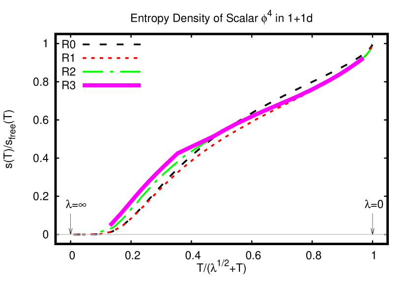
Figure 2: Entropy density as a function of re-scaled temperature $T/\sqrt{\lambda}$ for $m_{F}^{2}=\lambda$ in the R0-R3 approximation scheme. Results do not depend on the renormalization scale choice $\bar{\mu}$. Horizontal plot axis is expressed as $\frac{T}{T+\sqrt{\lambda}}$ to allow compactification of the whole interval $T\in[0,\infty)$. Arrows indicate location of weak and strong coupling regime $\lambda=0$, $\lambda=\infty$, respectively. Line thickness for R3 is representative for numerical errors arising from calculating numerical derivatives. The apparent “kink” in R3 at around $T\simeq 0.6$ is an artifact resulting from matching separately calculated values for the low and high temperature entropy, respectively. Full line is a guide to the eye. See text for details.

III Entropy density at finite temperature

The entropy density $s\equiv\frac{dP}{dT}$ is readily calculated from the expressions for the thermal pressure given in Eqns. (10), (15), respectively. One finds

$$s_{R0}(T),s_{R1}(T)=-\left.\frac{\partial J_{T}(M)}{\partial T}\right|_{M}=-\frac{M^{2}}{\pi T}\sum_{n=1}^{\infty}K_{2}\left(\frac{nM}{T}\right)\,,$$ (35)

where $M^{2}$ in the R0, R1 approximations is given in Eqns. (11), (16), respectively. While it is possible that also the R2- and R3-level approximation for the entropy density admits a simple expression, in practice one can calculate $s$ by performing a numerical temperature derivative from the existing results for the thermal pressure (24). Note that at low temperatures, taking the derivative becomes numerically more challenging, which is why results at very low temperature are not reported for R2, R3 here.

The results for the entropy density in the R0-R3 level approximations, normalized by the free entropy density result $s_{\rm free}=\frac{\pi T}{3}$ are shown in Fig. 2. As one can see from this figure, there is not only qualitative, but even overall quantitative agreement for the entropy density for all temperatures/couplings in the R0-R3 level approximations. Since R2 and R3 include the physics of thermal widths (albeit with different numerical factors), the fact that R2, R3 are close to the R0, R1 results for the entropy density may be taken as strong indication that thermal widths constitute a subleading effect to thermodynamic observables at any coupling strength.

If this result was valid in higher dimensions than 1+1d, this would be remarkable; it would suggest that when the physics of thermal widths is completely ignored, the resulting approximation schemes (R0, R1) give values for thermodynamic quantities which are good to better than 20 percent for all interaction strengths.

Leaving studies of this possibility for future work, given the approximate results for $s/s_{\rm free}$ for 1+1 dimensions shown in Fig. 2, I predict that exact calculations would give $s/s_{\rm free}>0.9$ for $T>21$ and $s/s_{\rm free}<0.2$ for $T<0.2$ for $m_{F}^{2}=1$. Based on the agreement between R0-R3, I expect these predictions to be robust.

Moreover, given that the R3 approximation was found to be quantitatively similar to high-precision results for scalar $\phi^{4}$ at zero temperature in Ref. Romatschke (2019), I predict that R3 results to be a good quantitative approximation to the exact result for $m_{F}^{2}=1$ for arbitrary temperatures/coupling values.

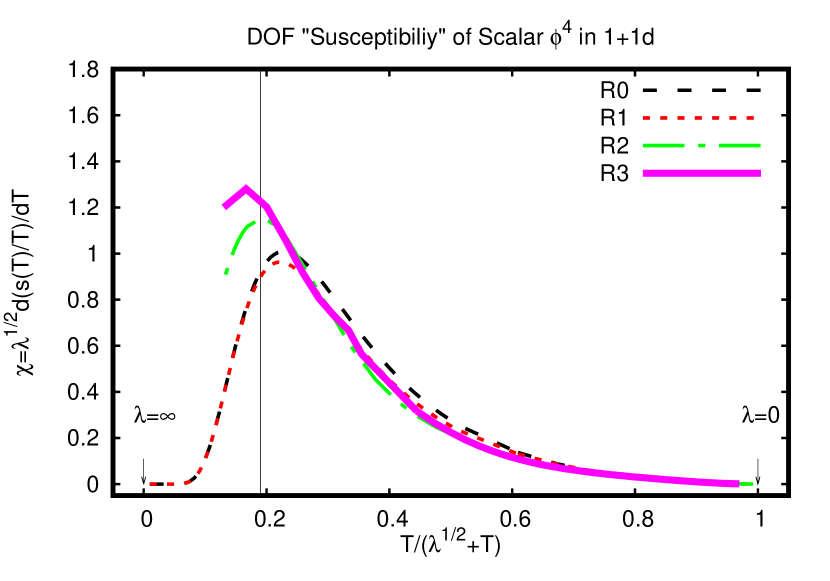
Figure 3: “Susceptibility” for the effective number of degrees of freedom (37) as a function of re-scaled temperature $T/\sqrt{\lambda}$ for $m_{F}^{2}=\lambda$ in the R0-R3 approximation scheme. Results do not depend on the renormalization scale choice $\bar{\mu}$. Horizontal plot axis is expressed as $\frac{T}{T+\sqrt{\lambda}}$ to allow compactification of the whole interval $T\in[0,\infty)$. Arrows indicate location of weak and strong coupling regime $\lambda=0$, $\lambda=\infty$, respectively. Line thickness for R3 is representative for numerical errors arising from calculating numerical derivatives. The apparent “kink” in R3 at around $T\simeq 0.6$ is an artifact resulting from matching separately calculated values for the low and high temperature entropy, respectively. Vertical line at $T\simeq 0.235$ is a guide to the eye. See text for details.

IV Cross-over transition between low and high temperature

The behavior of the entropy density as a function of temperature, normalized to the free-field result as shown in Fig. 2, bears similarities with that of full QCD in that there is a low-temperature regime where $s\simeq 0$ and a high-temperature regime where the entropy density approaches $s_{\rm free}$ from below. In QCD, the change in the normalized entropy density is associated with the change in the number of degrees of freedom from the confined low-temperature hadronic phase to the deconfined high-temperature quark-gluon plasma phase. Unlike pure Yang-Mills, the transition between confined and deconfined phase in full QCD with physical quark masses is known to be an analytic cross-over transition from lattice Monte-Carlo simulations Aoki et al. (2006).

In the absence of a true transition, there is no true order parameter characterizing the low- and high-temperature phase. However, approximate order parameters such as the effective number of degrees of freedom given by

$${\rm DOF}(T)=\frac{s(T)}{s_{\rm free}}\,,$$ (36)

in practice allow one to distinguish between the two phases. The location of the cross-over transition between low- and high- temperature “phase” may therefore be estimated from the peak of the “susceptibility”

$$\chi(T)\equiv\frac{d}{dT}{\rm DOF}(T)\,.$$ (37)

While there is no confinement mechanism operating in scalar field theory, one may nevertheless evaluate $\chi(T)$ for the R0-R3 approximations in order to distinguish between a low-temperature “phase” where $s\simeq 0$ and a high-temperature “phase” where $s\rightarrow s_{\rm free}$. The corresponding plot is shown in Fig. 3, indicating a broad cross-over transition at $T\simeq 0.235$ for $m_{F}^{2}=1$.

V Speed of Sound at finite temperature

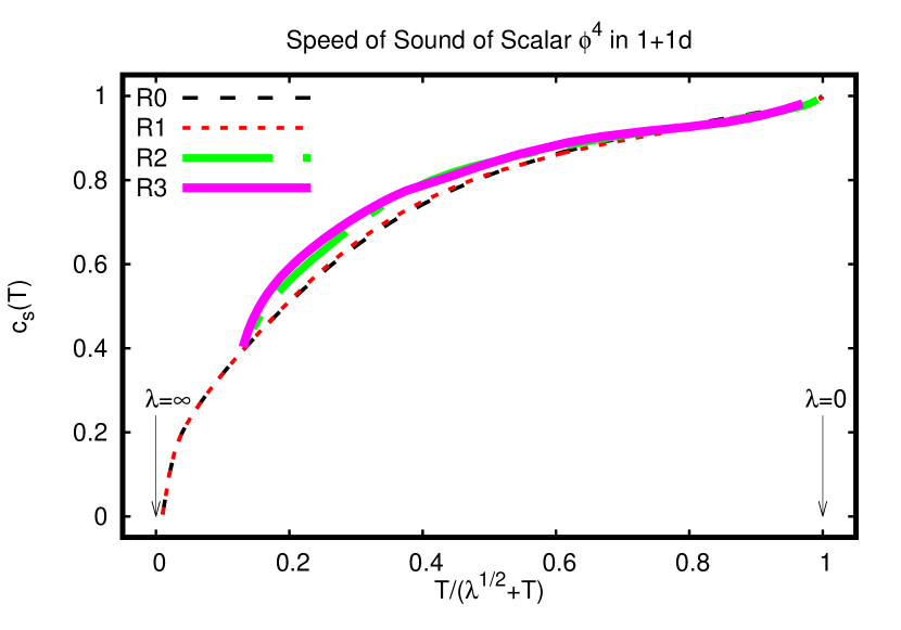
Figure 4: Speed of sound $c_{s}(T)$ as a function of re-scaled temperature $T/\sqrt{\lambda}$ for $m_{F}^{2}=\lambda$ in the R0-R3 approximation scheme. Results do not depend on the renormalization scale choice $\bar{\mu}$. Horizontal plot axis is expressed as $\frac{T}{T+\sqrt{\lambda}}$ to allow compactification of the whole interval $T\in[0,\infty)$. Arrows indicate location of weak and strong coupling regime $\lambda=0$, $\lambda=\infty$, respectively. Line thickness for R2- and R3-level results is representative for numerical errors arising from calculating numerical derivatives. The apparent “kink” in R3 at around $T\simeq 0.6$ is an artifact resulting from matching separately calculated values for the low and high temperature entropy, respectively. See text for details.

The speed of sound $c_{s}(T)$ at finite temperature is calculated from the thermodynamic relation

$$c_{s}(T)\equiv\sqrt{\frac{d\epsilon}{dP}}=\sqrt{\frac{s/T}{\frac{ds}{dT}}}\,,$$ (38)

where $\epsilon=sT-P$ is the energy density. The corresponding derivative of the entropy density is readily calculated numerically and one finds the speed of sound in the R0-R3 level approximation shown in Fig. 4. Similar to what has been found for the entropy density, the relative differences between R0-R3 for $c_{s}(T)$ are small for all temperatures/couplings shown. (Note that taking the second derivative of the pressure is numerically more difficult at low temperatures, which is why results for $c_{s}(T)$ are not reported for the lowest temperatures for R2, R3.)

VI Summary and Conclusions

In this work, I calculated thermodynamic properties for scalar $\phi^{4}$ in 1+1 dimensions at all temperatures/coupling values based on the non-perturbative resummation schemes R0-R3 developed in Ref. Romatschke (2019).

Results found for the thermal pressure, entropy density and speed of sound in the R0-R3 scheme were found to be well-behaved for arbitrary temperature and coupling strength. Furthermore, the dependence on the renormalization scale choice $\bar{\mu}\in[\pi T,4\pi T]$ dropped out explicitly for observables calculated in R0-R3. Moreover, results obtained in the R0-R3 schemes were also found to be numerically close at all temperatures/ coupling values. When contrasted with usual perturbation theory, these findings strongly suggest that the R0-R3 schemes are capable of providing quantitatively useful results for scalar $\phi^{4}$ theory even in the full non-perturbative regime.

In addition, the rapid rise of the entropy density as a function of temperature found in the R0-R3 calculations for $m_{F}^{2}=1$ hints at the possibility of an analytic cross-over between a low temperature and high temperature “phase” in scalar $\phi^{4}$ theory.

Given that scalar $\phi^{4}$ theory is amenable to direct numerical simulation using Monte Carlo lattice field theory techniques, I would encourage calculation of these thermodynamic observables on the lattice in the future.

VII Acknowledgments

This work was supported by the Department of Energy, DOE award No DE-SC0017905. I would like to thank P. Bedaque and M. Pinto for helpful discussions.

References

- Romatschke (2019) Paul Romatschke, “Simple non-perturbative resummation schemes beyond mean-field: case study for scalar theory in 1+1 dimensions,” (2019), arXiv:1901.05483 [hep-th] .
- Laine and Vuorinen (2016) Mikko Laine and Aleksi Vuorinen, “Basics of Thermal Field Theory,” Lect. Notes Phys. 925, pp.1–281 (2016), arXiv:1701.01554 [hep-ph] .
- Braaten and Pisarski (1990a) Eric Braaten and Robert D. Pisarski, “Soft Amplitudes in Hot Gauge Theories: A General Analysis,” Nucl. Phys. B337, 569–634 (1990a).
- Taylor and Wong (1990) J. C. Taylor and S. M. H. Wong, “The Effective Action of Hard Thermal Loops in QCD,” Nucl. Phys. B346, 115–128 (1990).
- Braaten and Pisarski (1990b) Eric Braaten and Robert D. Pisarski, “Deducing Hard Thermal Loops From Ward Identities,” Nucl. Phys. B339, 310–324 (1990b).
- Braaten and Pisarski (1992) Eric Braaten and Robert D. Pisarski, “Simple effective Lagrangian for hard thermal loops,” Phys. Rev. D45, R1827 (1992).
- Braaten and Yuan (1991) Eric Braaten and Tzu Chiang Yuan, “Calculation of screening in a hot plasma,” Phys. Rev. Lett. 66, 2183–2186 (1991).
- Kelly et al. (1994) P. F. Kelly, Q. Liu, C. Lucchesi, and C. Manuel, “Classical transport theory and hard thermal loops in the quark - gluon plasma,” Phys. Rev. D50, 4209–4218 (1994), arXiv:hep-ph/9406285 [hep-ph] .
- Flechsig and Rebhan (1996) Fritjof Flechsig and Anton K. Rebhan, “Improved hard thermal loop effective action for hot QED and QCD,” Nucl. Phys. B464, 279–297 (1996), arXiv:hep-ph/9509313 [hep-ph] .
- Moore et al. (1998) Guy D. Moore, Chao-ran Hu, and Berndt Muller, “Chern-Simons number diffusion with hard thermal loops,” Phys. Rev. D58, 045001 (1998), arXiv:hep-ph/9710436 [hep-ph] .
- Carrington et al. (1999) Magaret E. Carrington, De-fu Hou, and Markus H. Thoma, “Equilibrium and nonequilibrium hard thermal loop resummation in the real time formalism,” Eur. Phys. J. C7, 347–354 (1999), arXiv:hep-ph/9708363 [hep-ph] .
- Andersen et al. (1999) Jens O. Andersen, Eric Braaten, and Michael Strickland, “Hard thermal loop resummation of the free energy of a hot gluon plasma,” Phys. Rev. Lett. 83, 2139–2142 (1999), arXiv:hep-ph/9902327 [hep-ph] .
- Bodeker et al. (2000) D. Bodeker, Guy D. Moore, and K. Rummukainen, “Chern-Simons number diffusion and hard thermal loops on the lattice,” Phys. Rev. D61, 056003 (2000), arXiv:hep-ph/9907545 [hep-ph] .
- Blaizot et al. (1999) J. P. Blaizot, Edmond Iancu, and A. Rebhan, “Selfconsistent hard thermal loop thermodynamics for the quark gluon plasma,” Phys. Lett. B470, 181–188 (1999), arXiv:hep-ph/9910309 [hep-ph] .
- Bolz et al. (2001) M. Bolz, A. Brandenburg, and W. Buchmuller, “Thermal production of gravitinos,” Nucl. Phys. B606, 518–544 (2001), [Erratum: Nucl. Phys.B790,336(2008)], arXiv:hep-ph/0012052 [hep-ph] .
- Karsch et al. (2001) F. Karsch, M. G. Mustafa, and M. H. Thoma, “Finite temperature meson correlation functions in HTL approximation,” Phys. Lett. B497, 249–258 (2001), arXiv:hep-ph/0007093 [hep-ph] .
- Peshier (2001) Andre Peshier, “HTL resummation of the thermodynamic potential,” Phys. Rev. D63, 105004 (2001), arXiv:hep-ph/0011250 [hep-ph] .
- Blaizot et al. (2001a) J. P. Blaizot, Edmond Iancu, and A. Rebhan, “Approximately selfconsistent resummations for the thermodynamics of the quark gluon plasma. 1. Entropy and density,” Phys. Rev. D63, 065003 (2001a), arXiv:hep-ph/0005003 [hep-ph] .
- Blaizot et al. (2001b) J. P. Blaizot, Edmond Iancu, and A. Rebhan, “Quark number susceptibilities from HTL resummed thermodynamics,” Phys. Lett. B523, 143–150 (2001b), arXiv:hep-ph/0110369 [hep-ph] .
- Blaizot and Iancu (2002) Jean-Paul Blaizot and Edmond Iancu, “The Quark gluon plasma: Collective dynamics and hard thermal loops,” Phys. Rept. 359, 355–528 (2002), arXiv:hep-ph/0101103 [hep-ph] .
- Rebhan and Romatschke (2003) A. Rebhan and P. Romatschke, “HTL quasiparticle models of deconfined QCD at finite chemical potential,” Phys. Rev. D68, 025022 (2003), arXiv:hep-ph/0304294 [hep-ph] .
- Romatschke and Strickland (2003) Paul Romatschke and Michael Strickland, “Collective modes of an anisotropic quark gluon plasma,” Phys. Rev. D68, 036004 (2003), arXiv:hep-ph/0304092 [hep-ph] .
- Kraemmer and Rebhan (2004) Ulrike Kraemmer and Anton Rebhan, “Advances in perturbative thermal field theory,” Rept. Prog. Phys. 67, 351 (2004), arXiv:hep-ph/0310337 [hep-ph] .
- Andersen and Strickland (2005) Jens O. Andersen and Michael Strickland, “Resummation in hot field theories,” Annals Phys. 317, 281–353 (2005), arXiv:hep-ph/0404164 [hep-ph] .
- Rebhan et al. (2005) Anton Rebhan, Paul Romatschke, and Michael Strickland, “Hard-loop dynamics of non-Abelian plasma instabilities,” Phys. Rev. Lett. 94, 102303 (2005), arXiv:hep-ph/0412016 [hep-ph] .
- Laine et al. (2007) M. Laine, O. Philipsen, P. Romatschke, and M. Tassler, “Real-time static potential in hot QCD,” JHEP 03, 054 (2007), arXiv:hep-ph/0611300 [hep-ph] .
- Caron-Huot and Moore (2008) Simon Caron-Huot and Guy D. Moore, “Heavy quark diffusion in perturbative QCD at next-to-leading order,” Phys. Rev. Lett. 100, 052301 (2008), arXiv:0708.4232 [hep-ph] .
- Rychkov and Strumia (2007) Vyacheslav S. Rychkov and Alessandro Strumia, “Thermal production of gravitinos,” Phys. Rev. D75, 075011 (2007), arXiv:hep-ph/0701104 [hep-ph] .
- Ghiglieri et al. (2013) Jacopo Ghiglieri, Juhee Hong, Aleksi Kurkela, Egang Lu, Guy D. Moore, and Derek Teaney, “Next-to-leading order thermal photon production in a weakly coupled quark-gluon plasma,” JHEP 05, 010 (2013), arXiv:1302.5970 [hep-ph] .
- Haque et al. (2014) Najmul Haque, Aritra Bandyopadhyay, Jens O. Andersen, Munshi G. Mustafa, Michael Strickland, and Nan Su, “Three-loop HTLpt thermodynamics at finite temperature and chemical potential,” JHEP 05, 027 (2014), arXiv:1402.6907 [hep-ph] .
- Gorda et al. (2018) Tyler Gorda, Aleksi Kurkela, Paul Romatschke, Matias Säppi, and Aleksi Vuorinen, “Next-to-Next-to-Next-to-Leading Order Pressure of Cold Quark Matter: Leading Logarithm,” Phys. Rev. Lett. 121, 202701 (2018), arXiv:1807.04120 [hep-ph] .
- Aharony et al. (2004) Ofer Aharony, Joe Marsano, Shiraz Minwalla, and Toby Wiseman, “Black hole-black string phase transitions in thermal 1+1 dimensional supersymmetric Yang-Mills theory on a circle,” Class. Quant. Grav. 21, 5169–5192 (2004), arXiv:hep-th/0406210 [hep-th] .
- Kawahara et al. (2007) Naoyuki Kawahara, Jun Nishimura, and Shingo Takeuchi, “High temperature expansion in supersymmetric matrix quantum mechanics,” JHEP 12, 103 (2007), arXiv:0710.2188 [hep-th] .
- Hanada and Romatschke (2017) Masanori Hanada and Paul Romatschke, “Lattice Simulations of 10d Yang-Mills toroidally compactified to 1d, 2d and 4d,” Phys. Rev. D96, 094502 (2017), arXiv:1612.06395 [hep-th] .
- Serone et al. (2018) Marco Serone, Gabriele Spada, and Giovanni Villadoro, “ Theory I: The Symmetric Phase Beyond NNNNNNNNLO,” JHEP 08, 148 (2018), arXiv:1805.05882 [hep-th] .
- Elias-Miro et al. (2017) Joan Elias-Miro, Slava Rychkov, and Lorenzo G. Vitale, “High-Precision Calculations in Strongly Coupled Quantum Field Theory with Next-to-Leading-Order Renormalized Hamiltonian Truncation,” JHEP 10, 213 (2017), arXiv:1706.06121 [hep-th] .
- (37) P. Romatschke, “Numerical codes for theory in 1+1 dimensions at R2/R3 level,” https://github.com/paro8929/Resummation .
- Aoki et al. (2006) Y. Aoki, G. Endrodi, Z. Fodor, S. D. Katz, and K. K. Szabo, “The Order of the quantum chromodynamics transition predicted by the standard model of particle physics,” Nature 443, 675–678 (2006), arXiv:hep-lat/0611014 [hep-lat] .