Boundedness of a class of discretized reaction-diffusion systems

Abstract

Although the spatially continuous version of the reaction-diffusion equation has been well studied, in some instances a spatially-discretized representation provides a more realistic approximation of biological processes. Indeed, mathematically the discretized and continuous systems can lead to different predictions of biological dynamics. It is well known in the continuous case that the incorporation of diffusion can cause diffusion-driven blow-up with respect to the $L^{\infty}$ norm. However, this does not imply diffusion-driven blow-up will occur in the discretized version of the system. For example, in a continuous reaction-diffusion system with Dirichlet boundary conditions and nonnegative solutions, diffusion-driven blow up occurs even when the total species concentration is non-increasing. For systems that instead have homogeneous Neumann boundary conditions, it is currently unknown whether this deviation between the continuous and discretized system can occur. Therefore, it is worth examining the discretized system independently of the continuous system. Since no criteria exist for the boundedness of the discretized system, the focus of this paper is to determine sufficient conditions to guarantee the system with diffusion remains bounded for all time. We consider reaction-diffusion systems on a 1D domain with homogeneous Neumann boundary conditions and non-negative initial data and solutions. We define a Lyapunov-like function and show that its existence guarantees that the discretized reaction-diffusion system is bounded. These results are considered in the context of three example systems for which Lyapunov-like functions can and cannot be found.

34C11, 35K57, 37B25, 37F99, 65N40

1 Introduction

The reaction-diffusion (RD) modeling framework is used in biological and ecological literature to understand how systems with spatial dependencies evolve over time [22]. This equation is used, for example, to describe spatial population dynamics and phenomena such as pattern formation. Although the spatially-continuous RD equation is often studied, in some instances the spatially-discretized system allows for a more accurate representation of biological dynamics. For example, the discretized system is used to model patchy habitats in ecology [1, 8] and may prove useful in studying the effects of metabolic compartmentalization [28]. It is worth investigating the discretized system because the dynamics may differ significantly from the continuous system. For example in RD systems with Dirichlet boundary conditions, even when the total mass is conserved (i.e., the $L^{1}$ norm is bounded) the system may blow up in $L^{\infty}$ [23]. This implies that the discretized and continuous RD systems behave differently.

The existence of extensive literature discussing diffusion-driven blow up for the spatially-continuous system demonstrates that the question of boundedness is nontrivial (for a review see [6]). It is a known phenomenon that the addition of diffusion can affect the stability of steady-states leading to, for example, pattern formation, but the instability may also lead to unbounded solutions [6, 19, 27, 15]. Boundedness results for the continuous RD system have been obtained using duality arguments, Sobolev embedding theorems, and Lyapunov-type structures [17, 12, 16, 7]. However, to the best of our knowledge, our work is the first that derives conditions to guarantee the discretized RD system is uniformly bounded for all time.

Our approach is based on previous work that used the existence of a Lyapunov-type function to prove that the continuous RD system is uniformly bounded [17]. The Lyapunov-type function was required to be radially unbounded, additively separable, convex, and decreasing along solution trajectories. Here, we define a similar function, which we denote as a Lyapunov-like function (LLF), but replace the requirement of separability with more general conditions. Ultimately, the criteria placed on the LLF allows us to obtain boundedness results for systems with diffusion-driven instabilities.

We examine systems that have two species reacting and diffusing, homogeneous Neumann boundary conditions, and guaranteed non-negativity of solutions. Homogeneous Neumann boundary conditions are arguably more realistic for modeling compartments in biological systems then Dirichlet conditions. Additionally, since we are interested in diffusion-driven blow up, our focus will be on systems that have bounded solutions in reaction-only case. Under these conditions, diffusion-driven blow up has been shown to occur in the spatially-continuous system when the kinetics have a globally stable steady-state [26] and when there is a clear biological application [14] (i.e., modeling mutualistic populations in ecology).

In this work we present and prove sufficient conditions for the discretized version of the RD system to be uniformly bounded over time. In Section 2 we present relevant notation and define the properties of a LLF. In Section 3 we prove that the existence of this LLF guarantees the discretized RD system is uniformly bounded over time. In Section 4 we consider the results in the context of three examples that have well been well studied in the spatially-continuous case. For the first example, the continuous system has a bounded diffusion-driven instability, and, in the second two examples, the continuous systems can blow up in finite time. It is worth studying these examples in the discretized setting because it is unknown whether, generally, the continuous and discretized systems have the same boundedness properties. In Section 5 we conclude with a discussion of other applications and ideas for future directions.

2 Notation and definitions

We are interested in RD systems on the normalized spatial interval $I=[0,1]$ with two species $u$ and $v$. We will discretize this system with respect to space by creating $n$ spatial compartments, where $\mathscr{\mathcal{N}}=\{1,2,..,n\}$ represents the set of compartment indices (Figure 1).

Figure 1: Discretized system with $n$ spatial compartments. Reactions $f$ and $g$ occur within each compartment, and diffusion occurs between adjacent compartments.

Let $h$ denote the uniform width of each compartment and $x_{0},x_{1},...,x_{n}$ denote the compartment edges (i.e., $x_{i}=ih$ where $h=1/n$). Let $\mathbf{u}=(u_{1},u_{2},...,u_{n})^{T}$ and $\mathbf{v}=(v_{1},v_{2},...,v_{n})^{T}$ represent the average concentration of $u$ and $v$ in each of the $n$ spatial compartments, where these concentrations are assumed to be dimensionless. Let $\mathbf{f}(\mathbf{u},\mathbf{v})=(f(u_{1},v_{1}),f(u_{2},v_{2}),...,f(u_{n},v_{n}))^{T}$ and $\mathbf{g}(\mathbf{u},\mathbf{v})=(g(u_{1},v_{1}),g(u_{2},v_{2}),...,g(u_{n},v_{n}))^{T}$ represent the reactions taking place in each compartment. We will model diffusion as a Fickian flux between two adjacent compartments and, therefore, define

(1) $$D:=\left[\begin{array}[]{lllll}\text{-}1&1&&&0\\ 1&\text{-}2&1\\ &\ddots&\ddots&\ddots\\ &&1&\text{-}2&1\\ 0&&&1&\text{-}1\end{array}\right]$$

as the centered finite-difference matrix with homogeneous Neumann boundary conditions.

This leads to the following initial value problem

(2) $$\mathbf{u}_{t} =\gamma\mathbf{f}(\mathbf{u},\mathbf{v})+\frac{1}{h^{2}}D\mathbf{u}$$

$$\mathbf{v}_{t} =\gamma\mathbf{g}(\mathbf{u},\mathbf{v})+\frac{1}{h^{2}}dD\mathbf{v}$$

$$u_{i}(0) =u_{i,0} \text{for }i=1,2,...,n$$

$$v_{i}(0) =v_{i,0} \text{for }i=1,2,...,n$$

where $\gamma>0$ and $d>0$ are constants that are related to the size of the domain and the diffusion coefficients (see [19] for a discussion of these parameters). To guarantee non-negativity of solutions, we will require that $u_{i,0}\geq 0$, $v_{i,0}\geq 0$ for all $i\in\mathcal{N}$ and $f(0,v)\geq 0$, $g(u,0)\geq 0$ for all $u,v\in[0,\infty)$. We will further require that $f$ and $g$ be continuously differentiable. For simplicity we will assume that the parameters are constant across space. This includes both reaction parameters (i.e., constants within the functions $f$ and $g$) as well as spatial parameters (i.e., $\gamma$ and $d$). Note that the results can be easily generalized to systems with spatially varying parameters. By the Picard-Lindelöf theorem, there is a $T_{max}>0$ such that a noncontinuable classical and unique solution to (2) exists for $t\in[0,T_{max})$ where it is possible that $T_{max}=\infty$. Since the solution is classical, we know that $\mathbf{u}(t)$ and $\mathbf{v}(t)$ are continuous for $t\in[0,T_{max})$ and if $T_{max}<\infty$, then an element of $\mathbf{u}(t)$ and/or $\mathbf{v}(t)$ becomes unbounded as $t\rightarrow T_{max}$. Thus, if the solution is bounded for $t\in[0,T_{max})$, then $T_{max}=\infty$.

Throughout the paper we will be using $\|\cdot\|:\mathbb{R}^{2}\rightarrow\mathbb{R}$ to represent the $l_{1}$-norm and we define the total species concentration as $\|(u,v)\|=u+v$. Furthermore, we will use variations of $L$ (e.g., $L$, $\widetilde{L}$, $L_{i}$) to represent arbitrary nonnegative constants.

2.1 Lyapunov-like function

In this section we will define a Lyapunov-like function (LLF) for the reactions $f$ and $g$ given in (2). We will later prove that the existence of this LLF guarantees that the discretized RD system (2) is uniformly bounded for all time. The classical definition of a Lyapunov function is a continuously differentiable, locally positive-definite, scalar function that decreases along solution trajectories in the neighborhood of a steady state. The LLF defined here will instead decrease along reaction trajectories (i.e., solutions when diffusion is not included) when the total species concentration surpasses a threshold value.

Throughout the paper we will use $W$ to denote a LLF. Let $W:\mathbb{R}_{\geq 0}^{2}\rightarrow\mathbb{\mathbb{R}}_{\geq 0}$ be a twice continuously differentiable function. To denote the partial derivative of $W$ with respect to $u$ and $v$ we will use the notation $\partial_{u}W$ and $\partial_{v}W$, respectively. We will use $(W)_{i}$, $(\partial_{u}W)_{i}$, and $(\partial_{v}W)_{i}$ to denote the value of $W$ and its partial derivatives evaluated in compartment $i$ (e.g., $(W)_{i}=W(u_{i},v_{i})$). Furthermore, we define the vectors $\mathbf{W}:=((W)_{1},(W)_{2}...(W)_{n})$, $\partial_{u}\mathbf{W}:=((\partial_{u}W)_{1},(\partial_{u}W)_{2},...,(\partial_{u}W)_{n})$, and $\partial_{v}\mathbf{W}:=((\partial_{v}W)_{1},(\partial_{v}W)_{2},...,(\partial_{v}W)_{n})$.

We say that $W$ is a LLF for the reactions $f$ and $g$ if $W$ satisfies five properties, denoted below as (P1)–(P5). These properties imply secondary properties on $W$, which we will also present below. We first state three of the required properties, i.e. (P1)–(P3). Notably (P1) is the only property that depends on the reactions $f$ and $g$.

1. There exists a $\text{$\underline{K}$}>0$ such that if $\|(u,v)\|\geq\text{$\underline{K}$}$ then

   (3) $$\left(\nabla W(u,v)\right)(f(u,v),g(u,v))^{T}\leq 0.$$

2. For all $(u,v)\in\mathbb{R}_{\geq 0}^{2}$ the second derivatives of $W$ are strictly positive,

   $$\partial_{uu}W(u,v) >0,\quad\partial_{vv}W(u,v)>0,$$

   and the mixed partial derivative is non-negative

   $$\partial_{uv}W(u,v)\geq 0.$$

3. As the total species concentration goes to infinity, the LLF approaches infinity:

   $$\lim_{\|(u,v)\|\rightarrow\infty}W(u,v)=\infty.$$

The requirement that (3) holds only if the total species concentration is large enough leads to a more complicated boundedness proof but allows for LLFs to exist for systems that have diffusion-driven instabilities.

An additively-separable Lyapunov type function with properties similar to (P1)–(P3) was used to obtain a boundedness result in the continuous case [17]. Notably requiring additive separability in addition to (P1)–(P3) would be sufficient for proving the boundedness results in this paper. However, we do not require the LLF to be additively separably because it does not simplify the proofs significantly. Indeed, the final two properties (P4), (P5) are more general than requiring separability of the LLF.

Before we present these final properties, we will provide some needed notation and secondary properties that follow from (P2), (P3). Variations of the letter $M$ (e.g., $M^{(L)}$, $M_{u}^{(L)}$, $M_{v}^{(L)}$) will be used to represent a maximum value of either $W$ or a partial derivative of $W$ in regions of $\mathbb{R}_{\geq 0}^{2}$ where $\|(u,v)\|$ is constant. For $L>0$ define

(4) $$M^{(L)} :=\max_{\|(u,v)\|=L}W(u,v)$$

$$M_{u}^{(L)} :=\max_{\|(u,v)\|=L}\partial_{u}W(u,v)$$

$$M_{v}^{(L)} :=\max_{\|(u,v)\|=L}\partial_{v}W(u,v).$$

For the partial derivatives of $W$, we will also consider what happens in the limit as $u$ or $v$ approaches infinity. Thus, we define

(5) $$M_{u}^{(\infty)}(v) :=\lim_{u\rightarrow\infty}\partial_{u}W(u,v)$$

$$M_{v}^{(\infty)}(u) :=\lim_{v\rightarrow\infty}\partial_{v}W(u,v).$$

By (P2) we know these limits either converge and exist or diverge to infinity.

In the following corollary we prove the existence of three additional constants, $\underline{u},\underline{v}$, and $K$, that will be used in Section 3.

Corollary 2.1.

Suppose $W:\mathbb{R}_{\geq 0}^{2}\rightarrow\mathbb{\mathbb{R}}_{\geq 0}$ is twice continuously differentiable. If $W$ satisfies (P2), the following property holds:

1. The parameters $M_{u}^{(L)}$, $M_{v}^{(L)}$ are monotonically increasing with respect to $L$.

If, in addition, $W$ satisfies (P3), then the following properties also hold:

1. There exists constants $\underline{u}$ and $\underline{v}$ such that $\partial_{u}W(u,v)>0$ for all $u\geq\text{$\underline{u}$}$ and $\partial_{v}W(u,v)>0$ for all $v\geq\underline{v}$.

2. There exists a $K\geq\max\left\{\text{$\underline{K}$},\text{$\underline{u}$},\underline{v}\right\}$ such that if $L<K$ then $M^{(L)}<M^{(K)}$.

For the proof of this corollary see Appendix A.

For the fourth property, we will consider level-sets of $W$ and how the tangent lines to the level-sets behave (Figure 2). For every point $(u,v)\in\mathbb{R}_{\geq 0}^{2}$ there exists a level set of $W$ and corresponding tangent line that intersects $(u,v)$. The following property describes how these tangent lines behave as the total species concentration becomes large.

1. For a fixed value of $u$, the level-set tangent lines do not become parallel to the $v$-axis in the limit as $v\rightarrow\infty$, i.e.,

   $$\sup_{v\geq\text{$\underline{v}$}}\left|\frac{\partial_{u}W(u,v)}{\partial_{v}W(u,v)}\right|<\infty\text{ for all }u.$$

   Similarly, for a fixed value of $v$, the level-set tangent lines do not become parallel to the $u$-axis as $u\rightarrow\infty$, i.e.,

   $$\sup_{u\geq\underline{u}} \left|\frac{\partial_{v}W(u,v)}{\partial_{u}W(u,v)}\right|<\infty\text{ for all }v.$$

From this property we immediately see that for all $L\geq 0$ the following constants exist and are finite:

(6) $$R_{u,L} :=\sup_{u\leq L,v\geq\underline{v}}\left|\frac{\partial_{u}W(u,v)}{\partial_{v}W(u,v)}\right|$$

$$R_{v,L} :=\sup_{v\leq L,u\geq\underline{u}}\left|\frac{\partial_{v}W(u,v)}{\partial_{u}W(u,v)}\right|.$$

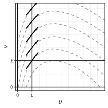
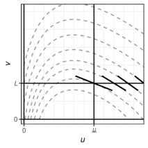
Figure 2: Graphical description of (P4). The dashed lines represent level sets of an example LLF and the black line segments represent tangent lines. Left: At $u=L$ and $v\geq\text{$\underline{v}$ }$the level-set tangent lines do not approach vertical. Right: At $v=L$ and $u\geq\text{$\underline{u}$ }$the level-set tangent lines do not approach horizontal.

For the final property, we place requirements on the limits of the partial derivatives of the LLF.

1. For all $v\in[0,\infty)$, either

   1. $M_{u}^{(\infty)}(v)$ is finite and $\lim_{u\rightarrow\infty}\partial_{uv}W(u,v)$ exists and is finite, or

   2. $M_{u}^{(\infty)}(v)$ is infinite.

   Similarly, for all $u\in[0,\infty)$, either

   1. $M_{v}^{(\infty)}(u)$ is finite and $\lim_{v\rightarrow\infty}\partial_{uv}W(u,v)$ exists and is finite, or

   2. $M_{v}^{(\infty)}(u)$ is infinite.

Now that we have stated all five properties, we will provide a formal definition of a LLF.

Definition 2.2.

Let $W:\mathbb{R}_{\geq 0}^{2}\rightarrow\mathbb{\mathbb{R}}_{\geq 0}$ be a twice continuously differentiable function. Consider the discretized system given by (2). Then $W$ is a LLF for this system if (P1)–(P5) are satisfied.

Finally, we will show that $M_{u}^{(\infty)}(v)$ and $M_{v}^{(\infty)}(u)$, given by (5), are constant functions and will therefore be referred to as $M_{u}^{(\infty)}$ and $M_{v}^{(\infty)}$, respectively.

Corollary 2.3.

The properties (P2), (P4), and (P5) imply the following secondary properties:

1. $M_{u}^{(\infty)}:=M_{u}^{(\infty)}(v)$ is independent of $v$ and $M_{u}^{(\infty)}>M_{u}^{(L)}$ for all $L\in[0,\infty)$.

2. $M_{v}^{(\infty)}:=M_{v}^{(\infty)}(u)$ is independent of $u$ and $M_{v}^{(\infty)}>M_{v}^{(L)}$ for all $L\in[0,\infty)$.

The proof of Corollary 2.3 is given in Appendix A.

In the remainder of this paper, we will reference the constants $K$, $\underline{u}$, and $\underline{v}$ given in Corollary 2.1. These constants only depend on the LLF. We will also reference the constants $M_{u}^{(L)}$, $M_{v}^{(L)}$, $M^{(L)}$, $R_{u,L}$ and $R_{v,L}$ given in (4), (5), and (6). These constants depend on both the LLF and the specified value of $L$.

2.2 Difference operator notation

Let $\mathbf{w}=(w_{1},w_{2},...,w_{n})^{T}$ be an arbitrary vector of length $n$. Define $\Delta_{i}^{+}$ and $\Delta_{i}^{-}$ as the forward and backward difference operator, respectively, where

$$\Delta_{i}^{+}\mathbf{\mathbf{\mathbf{w}}} :=w_{i+1}-w_{i}\text{ for }i=1,2,...,n-1$$

$$\Delta_{i}^{-}\mathbf{w} :=w_{i}-w_{i-1}\text{ for }i=2,3,...,n.$$

The $i$th element of the centered finite difference matrix, given by (1), acting on a vector $\mathbf{w}$ is given as

(7) $$(D\mathbf{w})_{i}=\begin{cases}\Delta_{1}^{+}\mathbf{w},&i=1\\ \Delta_{i}^{+}\mathbf{w}-\Delta_{i}^{-}\mathbf{w},&i=2,3,...,n-1\\ -\Delta_{n}^{-}\mathbf{w},&i=n.\end{cases}$$

Notice that for $i=1,n$ there is only a single term because we are assuming homogeneous Neumann boundary conditions. We will apply these difference operators to the species concentration vector, the LLF, and the partial derivatives of the LLF. For example, $\Delta_{i}^{+}\mathbf{W}=(W)_{i+1}-(W)_{i}$.

2.3 LLF $\Omega_{K}$ Region

To prove the main result, we will consider the following region of phase space (see Figure 3 for example):

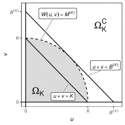
Figure 3: Illustration of example LLF $\Omega_{K}$ region and relevant constants. The dashed line represents the level set $W(u,v)=M^{(K)}$ and the shaded area is the $\Omega_{K}$ region.

$$\Omega_{K}:=\{(u,v)\in\mathbb{R}_{\geq 0}^{2}\mid W(u,v)<M^{(K)}\}.$$

Due to (C3) we know that $\Omega_{K}$ contains all points within the bounded region defined by the level set $W(u,v)=M^{(K)}$. Additionally, by (P1) we know that outside of this region, i.e. in $\Omega_{K}^{C}=\mathbb{R}_{\geq 0}^{2}\setminus\Omega_{K}$, (3) is satisfied. We will define the boundary of $\Omega_{K}$ as

$$\partial\Omega_{K}:=\{(u,v)\in\mathbb{R}_{\geq 0}^{2}\mid W(u,v)=M^{(K)}\}$$

where by definition $\Omega_{K}\cap\partial\Omega_{K}=\emptyset$. Define

(8) $$B^{(K)}:=\max_{(u,v)\in\partial\Omega_{K}}\|(u,v)\|.$$

We then know that for any compartment $i$ such that $(u_{i},v_{i})\in\Omega_{K}$, the total species concentration is bounded by $B^{(K)}$ (i.e., $\|(u_{i},v_{i})\|<B^{(K)}$).

2.4 Notation for the sum of Lyapunov-like functions

To consider the sum of LLFs across the spatial compartments, we will partition the set of compartments into those that are and are not contained in $\Omega_{K}$. Let the set $Y$ contain the indices of compartments that are in $\Omega_{K}$ and $Y^{C}$ contain the indices of compartments that are in $\Omega_{K}^{C}$ (i.e., $Y:=\{i\mid(u_{i},v_{i})\in\Omega_{K}\}$ and $Y^{C}=\mathcal{N}\setminus Y$ where recall that $\mathcal{N}=\{1,2,..,n\}$). Figure 4a,c gives an example of this notation (note that the sets $Z_{bdy}$ and $Z_{int}$ will be defined later in this section). For notational simplicity we will say that a compartment whose index is in $Y$ is a $Y$-compartment, and similarly, a compartment whose index is in $Y^{C}$ is a $Y^{C}$-compartment.

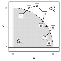
(a) Compartment location in phase space

(b) Compartment location in physical space

$$Y =\{1,5,7,8\}$$

$$Y^{C} =\{2,3,4,6\}$$

$$Z_{bdy} =\{1,4,5,6\}$$

$$Z_{int} =\{2,3\}$$

(c) Set of compartment/edge indices

Figure 4: Example notation for an 8 compartment system. In (b) $Y^{C}$-compartments are shaded in gray and the 7 edges are labeled by circles. There are four edges that separate a $Y$ from a $Y^{C}$-compartment (i.e., $|Z_{bdy}|=4$) and two edges that separate two $Y^{C}$ compartments (i.e., $|Z_{int}|=2$).

Suppose $X$ is either $Y$, $Y^{C}$, or $\mathcal{N}$ and define the sum of LLFs over indices in $X$ as the function $W_{X}:\mathbb{R}^{n}\times\mathbb{R}^{n}\rightarrow\mathbb{R}$ where

$$W_{X}(\mathbf{u},\mathbf{v}):=\sum_{i\in X}(W)_{i}.$$

When $X:=\mathcal{N}$ this equation will be referred to as the System LLF. Notice that $W_{\mathcal{N}}=W_{Y}+W_{Y^{C}}\leq nM^{(K)}+W_{Y^{C}}$. This implies that in order to bound $W_{\mathcal{N}}$, we need to find a bound on $W_{Y^{C}}$.

2.5 The LLF Evolution Equation

To bound $W_{Y^{C}}$, we will consider how its value evolves with time. Note that this evolution is piecewise continuous where the discontinuities occur when the membership of $Y^{C}$ changes. We will refer to such an event as a crossing of $\partial\Omega_{K}$. Compartment $i$ will have undergone a crossing at time $t$ if $i\in Y^{C}(t)$ and $i\in Y(t\pm\epsilon)$ for an arbitrary small $\epsilon>0$. If $i\in Y(t+\epsilon)$ then a crossing from $\Omega_{K}^{C}$ into $\Omega_{K}$ has occurred and if $i\in Y(t-\epsilon)$, a crossing from $\Omega_{K}$ into $\Omega_{K}^{C}$ has occurred.

In the notation that follows, we consider time periods when there are no crossings of $\partial\Omega_{K}$.We have that $W_{Y^{C}}$ is continuously differentiable and, therefore, we can define the LLF Evolution Equation as

$$\frac{dW_{Y^{C}}}{dt}=\left(\nabla_{\mathbf{u}}W_{Y^{C}}\right)\left(\frac{d\mathbf{u}}{dt}\right)^{T}+\left(\nabla_{\mathbf{v}}W_{Y^{C}}\right)\left(\frac{d\mathbf{v}}{dt}\right)^{T}$$

where $\nabla_{\mathbf{u}}W_{Y^{C}}=(\partial_{u_{1}}W_{Y^{C}},\partial_{u_{2}}W_{Y^{C}},...,\partial_{u_{n}}W_{Y^{C}})$ and $\nabla_{\mathbf{v}}W_{Y^{C}}$ is defined analogously. The LLF Evolution Equation tells us how the sum of LLFs over indices in $Y^{C}$ changes along solution trajectories.

We can divide the LLF evolution equation into reactive and diffusive flux contributions, i.e.,

$$\frac{dW_{Y^{C}}}{dt}=\gamma W_{Y^{C},R}+W_{Y^{C},D}$$

where

(9) $$W_{Y^{C},R} :=\left(\nabla_{\mathbf{u}}W_{Y^{C}}\right)\mathbf{f}(\mathbf{u},\mathbf{v})^{T}+\left(\nabla_{\mathbf{v}}W_{Y^{C}}\right)\mathbf{g}(\mathbf{u},\mathbf{v})^{T}$$

(10) $$W_{Y^{C},D} :=\left(\nabla_{\mathbf{u}}W_{Y^{C}}\right)D\mathbf{u}^{T}+\left(\nabla_{\mathbf{v}}W_{Y^{C}}\right)dD\mathbf{v}^{T}$$

represent the reactive and diffusive contribution, respectively.

2.6 The diffusive fluxes and compartment edges

We next examine the diffusive contribution to the LLF evolution equation, (10), by considering a more refined set of fluxes. We define an edge as the boundary between two adjacent compartments (see Figure 4b). Let $i=1,2,...,n-1$ denote an edge where the $i$th edge represents the boundary between the $i$ and $i+1$ compartment. We will call an edge that connects a $Y$ with a $Y^{C}$-compartment a boundary edge and an edge that connects two $Y^{C}$-compartments an interior edge. Note that we do not name the edges that connect two $Y$-compartments.

For each edge $i$ define the following

(11) $$n_{i}=\mathbf{1}_{Y}(i+1)-\mathbf{1}_{Y}(i)$$

where $\mathbf{1}$ is the indicator function. We then have that the sets

(12) $$Z_{bdy:} :=\left\{i\in\mathcal{N}\setminus\{n\}\mid\left|n_{i}\right|=1\right\}$$

$$Z_{int} :=\left\{i\in\mathcal{N}\setminus\{n\}\mid n_{i}=0\text{ and }i\in Y^{C}\right\}$$

contain the boundary edge indices and the interior edge indices, respectively. The maximum sizes of $Z_{bdy}$ and $Z_{int}$ are both $n-1$. Figure 4c defines $Z_{bdy}$ and $Z_{int}$ for an example system.

With this notation in mind, let’s again consider the diffusive contribution to the LLF Evolution Equation and rewrite (10) as a sum

(13) $$W_{Y^{C},D}=\sum_{i\in Y^{C}}\left(\partial_{u}W\right)_{i}\left(D\mathbf{u}\right)_{i}+d\left(\partial_{v}W\right)_{i}\left(D\mathbf{v}\right)_{i}.$$

Recall that $(D\mathbf{u})_{i}$ and $(D\mathbf{v})_{i}$ can be rewritten as shown in (7) and rewrite (13) as

(14) $$W_{Y^{C},D} =\sum_{i\in Z_{bdy}}F_{bdy,i}+\sum_{i\in Z_{int}}F_{int,i}$$

where

(15) $$F_{bdy,i} :=n_{i}\left((\partial_{u}W)_{i+\frac{1-n_{i}}{2}}\Delta_{i}^{+}\mathbf{u}+d(\partial_{v}W)_{i+\frac{1-n_{i}}{2}}\Delta_{i}^{+}\mathbf{v}\right)$$

(16) $$F_{int,i} :=-\left(\Delta_{i}^{+}\left(\partial_{u}\mathbf{W}\right)\Delta_{i}^{+}\mathbf{u}+d\Delta_{i}^{+}\left(\partial_{v}\mathbf{W}\right)\Delta_{i}^{+}\mathbf{v}\right).$$

We will refer to $F_{bdy,i}$ and $F_{int,i}$ as flux-effect terms because each represents the contribution of a single diffusive flux to the LLF Evolution Equation. In Section 3.1 we will show that, under certain conditions, the diffusive contribution to the LLF Evolution Equation is negative.

3 Boundedness theorems

We will prove the discretized RD system given by (2) is bounded if there exists a LLF for the reactions as described by Definition 2.2. The proof involves two main steps. In Section 3.1, we consider a snapshot of the system and show that if any compartment exceeds a threshold total species concentration, then the solution to the LLF Evolution Equation is decreasing. In Section 3.2, we consider the evolution of the system, and show that the System LLF is bounded. This bound on the System LLF in turn leads to a bound on the concentration of species within a single compartment.

3.1 At large species concentration the solution to the LLF Evolution Equation is nonincreasing

Recall that the LLF Evolution Equation can be broken down into the reactive (9) and diffusive (10) components. We know that the reactive component is nonpositive due to (P1). Thus, the main work of this section is to show that the diffusive component is nonpositive when a compartment exceeds a threshold species concentration.

The outline of the results in this section is given as follows. Recall that the diffusive component of the LLF Evolution Equation can be rewritten as a summation of flux-effect terms, as given by (14). Each of these flux-effect terms can be bounded from above by a constant (see Lemma 3.1). Therefore, the diffusive component is negative if there exists one negative flux-effect term with a sufficiently large magnitude. This negative flux-effect term exists if two adjacent compartments have a large enough difference between the amount of species they contain (see Lemma 3.3 and Corollary 3.5, 3.7, and 3.9). This difference in species concentration is obtained if there is at least one $Y$-compartment and one $Y^{C}$-compartment that exceeds a threshold species concentration (Lemma 3.11 and 3.13). It then immediately follows that the solution to the entire LLF Evolution Equation is nonincreasing (Corollary 3.15).

With this road-map in mind, we first show that the flux-effect terms $F_{bdy,i}$ and $F_{int,i}$ have an upper bound. By (P2) we immediately know that $F_{int,i}<0$ for all $i\in Z_{int}$. In the next lemma, we prove that $F_{bdy,i}$ has an upper bound as well.

Lemma 3.1.

Let $W$ by a LLF for the system given by (2). Suppose at an arbitrary time $t>0$, $Z_{bdy}$ is nonempty. Pick $i\in Z_{bdy}$ and let $F_{bdy,i}$ be as given in (15). Then there exists a constant $F_{max}$ such that $F_{bdy,i}\leq F_{max}$.

Proof 3.2.

Pick $i\in Z_{bdy}$ and recall $n_{i}$ is given by (11). We rewrite $F_{bdy,i}$ as follows:

$$F_{bdy,i}=n_{i}\left(F_{bdy,i}^{(u)}+F_{bdy,i}^{(v)}\right)$$

where

$$F_{bdy,i}^{(u)} :=(\partial_{u}W)_{i+\frac{1-n_{i}}{2}}\Delta_{i}^{+}\mathbf{u},\hskip 10.00002pt\hskip 10.00002pt\hskip 10.00002pt F_{bdy,i}^{(v)} :=d(\partial_{v}W)_{i+\frac{1-n_{i}}{2}}\Delta_{i}^{+}\mathbf{v}.$$

We will assume $n_{i}=1$ and note analogous logic can be applied if $n_{i}=-1$. Since $n_{i}=1$, $i+1\in Y$ and therefore

$$u_{i+1},v_{i+1},\Delta_{i}^{+}\mathbf{u},\Delta_{i}^{+}\mathbf{v}\leq B^{(K)}$$

where $B^{(K)}$ is given by (8).

For notational simplicity we define the following two constants:

$$u^{*} :=B^{(K)}\left(1+dR_{v,B^{(K)}}\right),\hskip 10.00002pt\hskip 10.00002pt v^{*} :=\frac{1}{d}B^{(K)}\left(d+R_{u,B^{(K)}}\right)$$

where $R_{v,B^{(K)}}$ and $R_{u,B^{(K)}}$ are given by (6). By (C3), $B^{(K)}>\underline{u},\underline{v}$, and thus $u^{*}\geq\underline{u}$ and $v^{*}\geq\underline{v}$.

We next consider three possible cases, one of which must occur. In the first case we bound $F_{bdy,i}$ directly and in the second two cases we bound $F_{bdy,i}^{(u)}$. First suppose $~{}\Delta_{i}^{+}\mathbf{u}\geq 0$ and $v_{i}>v^{*}$. Using (6) and (C2), we have that

$$F_{bdy,i} =(\partial_{v}W)_{i}\left(\frac{\left(\partial_{u}W\right)_{i}}{\left(\partial_{v}W\right)_{i}}\Delta_{i}^{+}\mathbf{u}+d\Delta_{i}^{+}\mathbf{v}\right)$$

$$\leq d(\partial_{v}W)_{i}\left(B^{(K)}\left(R_{u,B^{(K)}}+d\right)-dv^{*}\right)$$

$$\leq 0$$

Second, suppose $\Delta_{i}^{+}\mathbf{u}\geq 0$ and $v_{i}\leq$$v^{*}$. Using that $u_{i}<B^{(K)}$, we have that

$$F_{bdy,i}^{(u)} =(\partial_{u}W)_{i}\Delta_{i}^{+}\mathbf{u}$$

$$\leq\left(\max_{u\leq B^{(K)},v\leq v^{*}}\partial_{u}W(u,v)\right)B^{(K)}.$$

Third suppose $\Delta_{i}^{+}\mathbf{u}<0$. If $(\partial_{u}W)_{i}\leq 0$ then $u_{i}<\underline{u}$ and by (P2) we have that

$$F_{bdy,i}^{(u)} =\left|(\partial_{u}W)_{i}\right|\left|\Delta_{i}^{+}\mathbf{u}\right|$$

$$\leq\text{$\left|\partial_{u}W(0,0)\right|$}\underline{u}.$$

If instead $(\partial_{u}W)_{i}>0$, then $F_{bdy,i}^{(u)}<0$, and the given bound still holds.

These three cases imply that either

$$F_{bdy,i}\leq 0\quad\quad\text{ or $\quad\quad$}F_{bdy,i}^{(u)}\leq B^{(K)}\max_{u\leq B^{(K)},v\leq v^{*}}\left|\partial_{u}W(u,v)\right|.$$

We can analogously show that either $F_{bdy,i}\leq 0$ or $F_{bdy,i}^{(v)}$ is bounded from above by a constant. This leads to the final result that $F_{bdy,i}\leq F_{max}$ where

(17) $$F_{max}:=B^{(K)}\left(\max_{u\leq B^{(K)},v\leq v^{*}}\left|\partial_{u}W(u,v)\right|+d\max_{u\leq u^{*},v\leq B^{(K)}}\left|\partial_{v}W(u,v)\right|\right).$$

Our next goal is to show that under certain conditions one of the flux-effect terms that contributes to the LLF Evolution Equation, i.e., $F_{bdy,i}$ or $F_{int,i}$, is smaller than an arbitrary negative constant. We first pick an interior edge $\ell$ and show that the desired result is obtained when $\left|\Delta_{\ell}^{+}\mathbf{u}\right|$ or $\left|\Delta_{\ell}^{+}\mathbf{v}\right|$ is sufficiently large (Lemma 3.3 and Corollary 3.5). Furthermore, if there is a large enough difference in the total species concentration (i.e. $\left|\Delta_{\ell}^{+}(\textbf{$\mathbf{u}+\mathbf{v})$}\right|$) the desired result is obtained (Corollary 3.7) and similar results follow for an arbitrary boundary edge (Corollary 3.9). Below we will refer to compartment $\ell+1$ as compartment $\ell^{+}$.

Lemma 3.3.

Let $W$ be a LLF for the system given by (2). Pick an arbitrary time $t>0$ and suppose that $\ell\in Z_{int}$. Pick $A>0$ and $L>0$, where

$$\min\left\{\|(u_{\ell},v_{\ell})\|,\|(u_{\ell^{+}},v_{\ell^{+}})\|\right\}\leq L.$$

There exists a constant $G_{u}$ such that, if $\left|\Delta_{\ell}^{+}\mathbf{u}\right|\geq G_{u}$, then the flux-effect term for interior edge $\ell$ is bounded from above by $-A$, i.e. $F_{int,\ell}\leq-A$ where $F_{int,\ell}$ is given by (16) with $i:=\ell$.

Proof 3.4.

Pick $\widetilde{L}>L$ such that $M_{u}^{(\widetilde{L})}>0$. By (C4) this $\widetilde{L}$ exists and there is a $\widetilde{u}$ such that $\partial_{u}W(\widetilde{u},0)=M_{u}^{(\widetilde{L})}.$ Define the following two constants

$$C_{1} :=1-\frac{M_{u}^{(L)}}{M_{u}^{(\widetilde{L})}},\quad\quad C_{2}:=\left(R_{v,L}+\frac{\max_{\|(u,v)\|<L}|\partial_{v}W|}{M_{u}^{(\widetilde{L})}}\right)L$$

and let

(18) $$G_{u}:=\max\left\{\widetilde{u}+L,\frac{A+dM_{u}^{(\widetilde{L})}C_{2}}{M_{u}^{(\widetilde{L})}C_{1}}\right\}.$$

Notice that $C_{1},C_{2}>0$. The fact that $C_{1}>0$ follows from (C1).

Without loss of generality we will suppose that $\|(u_{\ell},v_{\ell})\|<\|(u_{\ell^{+}},v_{\ell^{+}})\|$ which implies $\|(u_{\ell},v_{\ell})\|<L$. Note that if $-\Delta_{\ell}^{+}\mathbf{u}\geq G_{u}$ then $u_{l}>G_{u}>L$, which is a contradiction. Therefore, $\Delta_{\ell}^{+}\mathbf{u}\geq G_{u}$ and by (C1),

(19) $$\max(0,M_{u}^{(L)})<M_{u}^{(\widetilde{L})}\leq(\partial_{u}W)_{\ell^{+}}<M_{u}^{(\infty)}.$$

The flux effect term $F_{int,\ell}$ can be rewritten as follows:

$$F_{int,\ell}=-(\partial_{u}W)_{\ell^{+}}\left(\frac{\Delta_{\ell}^{+}(\partial_{u}\mathbf{W})}{(\partial_{u}W)_{\ell^{+}}}\Delta_{\ell}^{+}\mathbf{u}+d\frac{\Delta_{\ell}^{+}(\partial_{v}\mathbf{W})}{(\partial_{u}W)_{\ell^{+}}}\Delta_{\ell}^{+}\mathbf{v}\right).$$

We will next examine the two terms in the parentheses that contribute to $F_{int,\ell}$. For the first term, using (19) gives the following bound:

$$\frac{\Delta_{l}^{+}\left(\partial_{u}\mathbf{W}\right)}{(\partial_{u}W)_{\ell^{+}}}\Delta_{\ell}^{+}\mathbf{u} =\left(1-\frac{(\partial_{u}W)_{\ell}}{(\partial_{u}W)_{\ell^{+}}}\right)\Delta_{\ell}^{+}\mathbf{u}\geq\left(1-\frac{M_{u}^{(L)}}{M_{u}^{(\widetilde{L})}}\right)G_{u}=C_{1}G_{u}$$

For the second term, first suppose that $\Delta_{\ell}^{+}\mathbf{v}\leq 0$. This implies that $v_{\ell^{+}},\left|\Delta_{\ell}^{+}\mathbf{v}\right|\leq L$ and leads to the following bound:

(20) $$d\frac{\Delta_{\ell}^{+}\left(\partial_{v}\mathbf{W}\right)}{(\partial_{u}W)_{\ell^{+}}}\Delta_{\ell}^{+}\mathbf{v} =-d\left(\frac{\left(\partial_{v}W\right)_{\ell^{+}}}{(\partial_{u}W)_{\ell^{+}}}-\frac{\left(\partial_{v}W\right)_{\ell}}{(\partial_{u}W)_{\ell^{+}}}\right)\left|\Delta_{\ell}^{+}\mathbf{v}\right|$$

$$\geq-d\left(R_{v,L}+\frac{\max_{\|(u,v)\|<L}|\partial_{v}W|}{M_{u}^{(\widetilde{L})}}\right)L=-dC_{2}.$$

If instead $\Delta_{\ell}^{+}\mathbf{v}>0$, then the left hand side of (20) is positive and, therefore, the bound still holds. The positivity of the left hand side follows from (19), which implies $(\partial_{u}W)_{\ell^{+}}>0$ and (P2), which implies $\Delta_{\ell}^{+}\left(\partial_{v}\mathbf{W}\right)\geq 0$. Finally, using (19)–(20) we have that

$$F_{int,\ell}\leq-M_{u}^{(\widetilde{L})}\left(C_{1}G_{u}-dC_{2}\right)\leq-A.$$

Corollary 3.5.

Suppose the assumptions of Lemma 3.3 hold. Given $A>0$ and $L>0$ where

$$\min\left\{\|(u_{\ell},v_{\ell})\|,\|(u_{\ell^{+}},v_{\ell^{+}})\|\right\}\leq L,$$

there exists a $G_{v}\geq L$ such that, if $\left|\Delta_{\ell}^{+}\mathbf{v}\right|\geq G_{v}$, then the flux-effect term for interior edge $\ell$ is bounded from above, i.e., $F_{int,\ell}\leq-A$ where $F_{int,\ell}$ is given by (16) with $i:=\ell$.

Proof 3.6.

The proof follows using the same logic as the proof to Lemma 3.3. First, find $\widetilde{L}>L$ such that $M_{v}^{(\widetilde{L})}>0$ and $\widetilde{v}$ such that $\partial_{v}(0,\widetilde{v})=M_{v}^{(\widetilde{L})}.$ Then define an analogous set of constants

$$C_{3}:=1-\frac{M_{v}^{(L)}}{M_{v}^{(\widetilde{L})}},\quad\quad C_{4}:=L\left(R_{u,L}+\frac{\max_{\|(u,v)\|<L}|\partial_{u}W(u,v)|}{M_{v}^{(\widetilde{L})}}\right)$$

and let

(21) $$G_{v}:=\max\left\{\widetilde{v}+L,\frac{A+M_{v}^{(\widetilde{L})}C_{4}}{dM_{v}^{(\widetilde{L})}C_{3}}\right\}.$$

We then have that $F_{int,\ell}\leq-M_{v}^{(\widetilde{L})}\left(-C_{4}+dC_{3}G_{v}\right)\leq-A.$

Corollary 3.7.

Suppose the assumptions of Lemma 3.3 hold. Given $A>0$ and $L>0$ where

$$\min\left(\|(u_{\ell},v_{\ell})\|,||(u_{\ell^{+}},v_{\ell^{+}})\|\right)\leq L,$$

there exists a $G\geq L$ such that if

(22) $$\Bigl{|}||(u_{\ell^{+}},v_{\ell^{+}})\|-\|(u_{\ell},v_{\ell})\|\Bigr{|}\geq G,$$

then $\max\left\{\|(u_{\ell},v_{\ell})\|,\|(u_{\ell^{+}},v_{\ell^{+}})\|\right\}>B^{(K)}$ and the flux-effect term for interior edge $\ell$ is bounded from above as follows

(23) $$F_{int,\ell}\leq-A$$

where $F_{int,\ell}$ is given by (16) with $i:=\ell$.

Proof 3.8.

Let

(24) $$G=\max\left\{2G_{u},2G_{v},B_{K}\right\}.$$

where $G_{u}$ is given by (18), $G_{v}$ is given by (21), and $B_{K}$ is given by (8). Notice that

$$\Bigl{|}||(u_{\ell^{+}},v_{\ell^{+}})\|-\|(u_{\ell},v_{\ell})\|\Bigr{|}=\left|\Delta_{\ell}^{+}\mathbf{u}+\Delta_{\ell}^{+}\mathbf{v}\right|$$

and, therefore, (22) and (24) imply that either $\left|\Delta_{\ell}^{+}\mathbf{u}\right|\geq G_{u}$ or $\left|\Delta_{\ell}^{+}\mathbf{v}\right|\geq G_{v}$. Thus, we apply either Lemma 3.3 or Corollary 3.5 to show that (23) holds. Finally, since $G\geq B_{K}$, using (22), we have that $\max\left\{\|(u_{\ell},v_{\ell})\|,\|(u_{\ell^{+}},v_{\ell^{+}})\|\right\}>B^{(K)}$.

Corollary 3.9.

Suppose the assumptions of Lemma 3.3 hold where instead we pick $\ell\in Z_{bdy}$. Given $A>0$ and $L>0$ where $\min\left(\|(u_{\ell},v_{\ell})\|,||(u_{\ell^{+}},v_{\ell^{+}})\|\right)\leq L$, find the $G$ from Corollary 3.7, given by (24). If (22) holds, then

$$\max\left\{\|(u_{\ell},v_{\ell})\|,\|(u_{\ell^{+}},v_{\ell^{+}})\|\right\}>B^{(K)}$$

and the flux-effect term for boundary edge $\ell$ is bounded from above as follows

(25) $$F_{bdy,\ell} \leq-A$$

where $F_{bdy,\ell}$ is given by (15) with $i:=\ell$.

Proof 3.10.

The result follows directly from Corollary 3.7. Without loss of generality again suppose $\|(u_{\ell^{+}},v_{\ell^{+}})\|>\|(u_{\ell},v_{\ell})\|.$ It immediately follows that $\|(u_{\ell^{+}},v_{\ell^{+}})\|\geq G\geq B^{(K)}$. This, in turn, implies that $\ell^{+}\in Y^{C}$ and hence $\ell\in Y$. The equation for $F_{bdy,\ell}$ then reduces to

$$F_{bdy,\ell}=-(\partial_{u}W)_{\ell^{+}}\Delta_{\ell}^{+}\mathbf{u}-d(\partial_{v}W)_{\ell^{+}}\Delta_{\ell}^{+}$$

To bound this equation, we apply the logic from Lemma 3.3, Corollary 3.5 and 3.7 where $(\partial_{u}W)_{\ell}$ and $(\partial_{v}W)_{\ell}$ are equal to zero. The result of this logic gives us that $F_{bdy,\ell}\leq-A$.

We will next assume the set $Y$ is not empty and show that when a threshold total species concentration is passed in at least one compartment, we can find a interior or boundary edge that satisfies either (23) or (25), respectively.

Lemma 3.11.

Let $W$ be a LLF for the system given by (2) and pick an arbitrary time $t>0$. Pick $A>0$ and suppose there exists a compartment $k$ such that $k\in Y$. Then there is a threshold concentration $C>0$ such that if $\max(\|(u_{i},v_{i})\|)_{i=1}^{n}\geq C$, then there exists an interior or boundary edge, $\ell$, that satisfies either (23) or (25), respectively.

Proof 3.12.

Suppose there does not exist an interior edge or boundary edge that satisfies either (23) or (25), respectively. The species concentration in compartment $k$ is bounded such that $\|(u_{k},v_{k})\|<B^{(K)}$. We will apply either Corollary 3.7 or 3.9 to iteratively bound the compartment concentration for $i=k+1,k+2,...,n$ and $i=k-1,k-2,...,1$.

Define $L_{k}:=B^{(K)}$ and, for $i=k+1,...,n$, iteratively find the $G_{i}$ given by (24) in Corollary 3.7 where $L:=L_{i-1}$. Next, set $L_{i}:=G_{i}+L_{i-1}$. If $\|(u_{i},v_{i})\|-\|(u_{i-1},v_{i-1})\|>G_{i}$ then edge $i$ is either an interior or boundary edge and, by Corollary 3.7 or 3.9 either (23) or (25) holds, resulting in a contradiction. Therefore, $\|(u_{i},v_{i})\|-\|(u_{i-1},v_{i-1})\|\leq G_{i}=L_{i}-L_{i-1}$, implying $\|(u_{i},v_{i})\|\leq L_{i}$. Thus, we have obtained an upper bound for the compartment $i$ and can continue the iteration. Similarly, for $i=k-1,...,1$, the same methodology can be used to generate compartment bounds, where we find the $G_{i}$ given by (24) where $L:=L_{i+1}$ .

This logic leads to the following bound

$$\|(u_{k+i},v_{k+i})\|<C$$

for $i=-k,...,-2,-1,1,2,..,n-k$ where the threshold species concentration $C$ is

(26) $$C:=B^{(K)}+\sum_{i=1,i\neq k}^{n}G_{i}.$$

Suppose that there exists a compartment $m$ such that $\|(u_{m},v_{m})\|\geq C$. We have a contradiction, and therefore there exists at least one interior or boundary edge such that either (23) or (25) holds.

In the next lemma we prove that if a compartment exceeds a threshold species concentration then the diffusive contribution to the LLF Evolution Equation is nonpositive (i.e., $W_{Y^{C},D}\leq 0$).

Lemma 3.13.

Let $W$ be a LLF for the system given by (2). Define $A:=nF_{max}$ where $F_{max}$ is given by (17) in Lemma 3.1. If we use this $A$ as the constant in Lemma 3.11, we can let $C$ be as defined in (26). If at an arbitrary time $t>0$, $\max_{i}\|(u_{i},v_{i})\|\geq C$, then $W_{Y^{C},D}\leq 0.$

Proof 3.14.

First suppose that $Y$ is empty. Then $Y^{C}=\mathcal{N}$ and

$$W_{Y^{C}}=\sum_{i=1}^{n}(W)_{i}.$$

The diffusion component of the LLF Evolution Equation is given as

$$W_{Y^{C},D} =\left(\nabla_{u}W_{Y^{C}}\right)D\mathbf{u}^{T}+d\left(\nabla_{v}W_{Y^{C}}\right)D\mathbf{v}^{T}$$

$$=\sum_{i=1}^{n-1}-\Delta_{i}^{+}(\partial_{u}\mathbf{W})\Delta_{i}^{+}\mathbf{u}-d\Delta_{i}^{+}(\partial_{v}\mathbf{W})\Delta_{i}^{+}\mathbf{v}$$

$$\leq 0.$$

This result follows from property (P2) of the LLF.

Next, suppose that $Y$ is not empty. By Lemma 3.11, there exists either an interior edge that satisfies (23) or a boundary edge that satisfies (25). We will let $\ell$ denote the index of this edge. We know $\max\left\{\|(u_{\ell},v_{\ell})\|,\|(u_{\ell^{+}},v_{\ell^{+}})\|\right\}>B^{(K)}$. Without loss of generality, suppose $\|(u_{\ell^{+}},v_{\ell^{+}})\|>\|(u_{\ell},v_{\ell})\|$ and thus $\ell^{+}\in Y^{C}$. We will next consider two possible cases: $\ell\in Z_{int}$ or $\ell\in Z_{bdy}$.

First let’s assume $\ell\in Z_{int}$. By Corollary 3.7, we have that

$$F_{int,\ell}\leq-nF_{max}.$$

Using that $F_{int,i}<0$ and $F_{bdy,i}\leq F_{max}$ for all $i$, and that $Z_{bdy}$ has at most $n-1$ elements, we have that

$$W_{Y^{C},D} =\sum_{i\in Z_{bdy}}F_{bdy,i}+\sum_{i\in Z_{int}}F_{int,i}$$

$$\leq\sum_{i\in Z_{bdy}}F_{bdy,i}+F_{int,\ell}$$

$$\leq(n-1)F_{max}-nF_{max}$$

$$<0.$$

Next, assume $\ell\in Z_{bdy}$. We have that by Corollary 3.9

$$F_{bdy,\ell}<-nF_{max}.$$

We then can similarly bound $W_{Z,D}$ as follows,

$$W_{Y^{C},D} =\sum_{i\in Z_{bdy}}F_{bdy,i}+\sum_{i\in Z_{int}}F_{int,i}$$

$$\leq F_{bdy,\ell}+\sum_{i\in Z_{bdy},i\neq\ell}F_{bdy,i}$$

$$\leq-nF_{max}+(n-2)F_{max}$$

$$<0.$$

Finally, we’ll prove the main result of this section. Specifically, we will next show that given a compartment exceeds a threshold species concentration, the solution to the LLF Evolution Equation is decreasing.

Corollary 3.15.

If the assumptions of Lemma 3.13 hold, then $\frac{dW_{Y^{C}}}{dt}\leq 0$.

Proof 3.16.

From Lemma 3.13 we know that $W_{Y^{C},D}\leq 0$. Furthermore, (9) can be rearranged as follows

$$W_{Y^{C},R}=\sum_{i\in Y^{C}}\left(\nabla W(u_{i},v_{i})\right)(f(u_{i},v_{i}),g(u_{i},v_{i}))^{T}.$$

This sum is clearly less than zero by (P1) of the LLF. Therefore,

$$\frac{dW_{Y^{C}}}{dt}=\gamma W_{Y^{C},R}+W_{Y^{C},D}\leq 0.$$

3.2 The System LLF is bounded

In this section we will consider how the System LLF or the sum of LLFs across all compartments evolves with time. We will first only consider times when one compartment exceeds a threshold species concentration. During these times we will consider what occurs to the System LLF when the membership of $Y$ and $Y^{C}$ changes. Below we define a time-dependent function that bounds the System LLF. We will show that this function decreases with time if any compartment exceeds a threshold total species concentration (Lemma 3.18). We conclude by considering all times during which a solution exists, i.e., $t\in[0,T_{max})$, and show that the given function will always bound the system. Hence, the total species concentration in each compartment is uniformly bounded over time (Theorem 3.20). Furthermore, since the solution does not blow up, we are guaranteed that $T_{max}=\infty$.

Consider the discretized RD system given by (2) and let $W:\mathbb{R}_{\geq 0}^{2}\rightarrow\mathbb{R}$ be a LLF for the reactions. Using this LLF and the initial data, we define the threshold species concentration $\underline{C}$ as follows.

Definition 3.17.

Find the $F_{max}$ for the LLF given by (17) in Lemma 3.1. Apply Lemma 3.11 where $A:=nF_{max}$ to find $C$. We then define the threshold species concentration as

$$\text{$\underline{C}$}=\max\left\{\left(\|(u_{i,0},v_{i,0})\|\right)_{i=1}^{n},C\right\}.$$

We will consider times during which the total species concentration in at least one compartment is greater than or equal to $\underline{C}$ and examine what occurs to the sum of LLFs when crossings of $\partial\Omega_{K}$ occur. Let $n_{t}$ be the number of compartments contained in $\Omega_{K}$ at time $t$ and define

(27) $$\mathcal{W}(t)=n_{t}M^{(K)}+W_{Y^{C}(t)}(\mathbf{u}(t),\mathbf{v}(t))$$

Note that $\mathcal{W}(t)$ provides an upper bound on the System LLF at time $t$.

We will first show that while the species concentration in at least one compartment exceeds $\underline{C}$, $\mathcal{W}(t)$ is a decreasing function of time. To do this we consider a closed interval of time, and allow for crossings of $\partial\Omega_{K}$ to occur at either end of the interval.

Lemma 3.18.

Pick $\tau_{1}$ and $\tau_{2}$ such that no crossings occur for $t\in\left(\tau_{1},\tau_{2}\right)$. Suppose for $t\in[\tau_{1},\tau_{2}]$, $\max\left\{\left(\|(u_{i},v_{i})\|\right)_{i=1}^{n}\right\}\geq\underline{C}$. Then,

(28) $$\mathcal{W}\left(\tau_{2}\right)\leq\mathcal{W}\left(\tau_{1}\right).$$

Proof 3.19.

We will first show how $W_{Y^{C}(\tau_{1})}(\mathbf{u}(\tau_{1}),\mathbf{v}(\tau_{1}))$ and $W_{Y^{C}(\tau_{2})}(\mathbf{u}(\tau_{2}),\mathbf{v}(\tau_{2}))$ are related. Notice that $Y(t)$ and $Y^{C}(t)$ do not have changes in membership for all $t\in\left(\tau_{1},\tau_{2}\right)$ since no crossings of $\partial\Omega_{K}$ occur. Pick $t\in(\tau_{1},\tau_{2})$. Corollary 3.15 along with the continuity of $\mathbf{u}$ and $\mathbf{v}$ imply that

(29) $$W_{Y^{C}(t)}(\mathbf{u}(\tau_{2}),\mathbf{v}(\tau_{2}))\leq W_{Y^{C}(t)}(\mathbf{u}(\tau_{1}),\mathbf{v}(\tau_{1})).$$

Let $n_{in}$ denote the number of compartments that cross into $\Omega_{K}$ at time $\tau_{1}$, and let $n_{out}$ denote the number of compartments that cross out of $\Omega_{K}$ at time $\tau_{2}.$ We have that

$$W_{Y^{C}\left(\tau_{1}\right)}\left(\mathbf{u}\left(\tau_{1}\right),\mathbf{v}\left(\tau_{1}\right)\right)=W_{Y^{C}(t)}\left(\mathbf{u}\left(\tau_{1}\right),\mathbf{v}\left(\tau_{1}\right)\right)+n_{in}M^{(K)}$$

and

$$W_{Y^{C}\left(\tau_{2}\right)}\left(\mathbf{u}\left(\tau_{2}\right),\mathbf{v}\left(\tau_{2}\right)\right)=W_{Y^{C}(t)}\left(\mathbf{u}\left(\tau_{2}\right),\mathbf{v}\left(\tau_{2}\right)\right)+n_{out}M^{(K)}$$

Using these relations and (29), we deduce the following inequality:

$$W_{Y^{C}\left(\tau_{2}\right)}\left(\mathbf{u}\left(\tau_{2}\right),\mathbf{v}\left(\tau_{2}\right)\right)\leq W_{Y^{C}\left(\tau_{1}\right)}\left(\mathbf{u}\left(\tau_{1}\right),\mathbf{v}\left(\tau_{1}\right)\right)+(n_{out}-n_{in})M^{(K)}.$$

Using (27) and $n_{\tau_{2}}=n_{\tau_{1}}+n_{in}-n_{out}$ gives us the final result since

$$\mathcal{W}\left(\tau_{2}\right) =\left(n_{\tau_{1}}+n_{in}-n_{out}\right)M^{(K)}+W_{Y^{C}(\tau_{2})}\left(\mathbf{u}\left(\tau_{2}\right),\mathbf{v}\left(\tau_{2}\right)\right)$$

$$\leq n_{\tau_{1}}M^{(K)}+W_{Y^{C}(\tau_{1})}\left(\mathbf{u}\left(\tau_{1}\right),\mathbf{v}\left(\tau_{1}\right)\right)$$

$$\leq\mathcal{W}\left(\tau_{1}\right).$$

Finally, we will prove our main result by considering how the system evolves for all time $t\in[0,T_{max})$.

Theorem 3.20.

Consider the ODE system given by (2), and suppose there exists a LLF $W:\mathbb{R}_{\geq 0}^{2}\rightarrow\mathbb{R}$ for this system Then, there exists an upper bound $B>0$ such that $\|(u_{i}(t),v_{i}(t))\|\leq B$ for $i=1,2,...,n$ and all $t\in[0,\infty)$.

Proof 3.21.

Pick $t\in[0,T_{max})$. Define $T^{(M)}$ as follows:

$$T^{(M)}=\left\{t\in[0,T_{max})\mid\max_{i=1,..,n}\left\{\|(u_{i}(t),v_{i}(t))\|\right\}\geq\underline{C}\right\}$$

where $\underline{C}$ is given by Definition 3.17. By the continuity of $u_{i}(t)$ and $v_{i}(t)$ we know that $T^{(M)}$ is a finite union of closed connected sets where

$$T^{(M)}=\bigcup_{i=1}^{m}T_{i}^{(M)}.$$

Pick $i=1,2,..,m$ and suppose there are $J$ crossings in $T_{i}^{(M)}$. Again, by the continuity of $u_{i}(t)$ and $v_{i}(t)$ we know that the number of crossings is finite. Let $t_{j}$, for $j=1,2,...,J$, denote the time at which crossings of $\partial\Omega_{K}$ occur and let $t_{0}$ and $t_{J+1}$ denote the start and end of the time interval, respectively (i.e., $T_{i}^{(M)}=[t_{0},t_{J+1}]$). We then have that

$$T_{i}^{(M)}=\bigcup_{j=0}^{J}[t_{j},t_{j+1}].$$

Pick $j=0,1,...,J$ and pick $\tau\in[j,j+1]$. Apply Lemma 3.18 to show

$$W_{\mathcal{\mathcal{N}}}(\mathbf{u}(\tau),\mathbf{v}(\tau)) \leq\mathcal{W}(\tau)\leq\mathcal{W}(t_{j})\leq\mathcal{W}(t_{j-1})\leq...$$

$$\leq\mathcal{W}(t_{0})=n_{t_{0}}M^{(K)}+W_{Y^{C}(t_{0})}(\mathbf{u}(t_{0}),\mathbf{v}(t_{0}))$$

From the definition of $t_{0}$, we know for all $i$, $\|(u_{i}(t_{0}),v_{i}(t_{0}))\|\leq\underline{C}$, and, therefore, $W(u_{i}(t_{0}),v_{i}(t_{0}))\leq M^{(\underline{C})}$. This follows from (P2), (C3), and the fact that $\underline{C}>K$ . The final bound we obtain is

(30) $$W_{\mathcal{N}}(\mathbf{u}(\tau),\mathbf{v}(\tau))\leq n_{t_{0}}M^{(K)}+(n-n_{t_{0}})M^{(\underline{C})}\leq nM^{(\underline{C})}.$$

Note that since $j$ and $i$ were arbitrary the same bound holds for all $\tau\in T^{(M)}$. Furthermore, for $\tau\leq t$ such that $\tau\notin T^{(M)}$ we know that $W(u_{i}(t_{0}),v_{i}(t_{0}))\leq M^{(\underline{C})}$ for $i=1,2,...,n.$ Thus, the bound given by (30) still holds. Finally, since $t$ was arbitrary this bound holds for all $t\in[0,T_{max})$.

Define $\Omega=\{(u,v)\mid W(u,v)\leq nM^{(\underline{C})}\}$. By (30) $(u_{i}(t),v_{i}(t))\in\Omega$ for all $i\in\{1,2,..,n\}$ and $t\in[0,T_{max})$. This implies that the total species concentration in each compartment is bounded by $B$ where

$$B=\max_{(u,v)\in\Omega}\|(u,v)\|$$

and $T_{max}=\infty$.

4 Applications: General results and example systems

Here, we discuss how to apply the boundedness results from Section 3. We first present some general rules that can be used to help determine whether an LLF exists for a specific reaction set. We then present three example systems that illustrate how diffusion-driven instability can lead to both bounded and unbounded solutions. These examples illustrate that, although diffusion-driven blow up can occur in the spatially-discretized system, Theorem 3.20 can be applied to find systems for which this is not the case.

4.1 General rules for determining whether a LLF exists

In some cases it is possible to quickly find a candidate LLF or to show an LLF cannot exist. If a known Lyapunov function exists for the reactions, it may also satisfy the requirements of a LLF. By definition, any global Lyapunov function satisfies (P1) and (P3). Therefore, it remains to show that a specific Lyapunov function satisfies (P2), (P4), and (P5). In the following corollary, we show that if the Lyapunov function is additively separable and satisfies (P2) then (P4) and (P5) follow.

Corollary 4.1.

Let $W:\mathbb{R}_{\geq 0}^{2}\rightarrow\mathbb{R}_{\geq 0}$ by a Lyapunov function for the reactions $f(u,v)$ and $g(u,v)$. If, in addition $W$ is additively separable (i.e., $W(u,v)=w_{1}(u)+w_{2}(v)$) and satisfies (P2), then $W$ is a LLF.

The proof of this corollary is given in A.4. As an example application of Corollary 4.1, consider a Lyapunov function consisting of a positive monomial for $u$ and $v$ with degree $\geq 2$ (i.e., $W(u,v)=\alpha u^{m}+\beta v^{p}$ where $\alpha,\beta\in\mathbb{R_{+}}$ and $m,p=2,3,...$). It follows immediately from Corollary 4.1 that $W$ is a LLF.

In some cases, it is possible to quickly determine that no LLF exists for a system. In the next corollary, we present conditions on the reactions $f$ and $g$ in (2) that guarantee a LLF for the system cannot be found.

Corollary 4.2.

Consider the system given by (2). If for any $v\geq 0$ the following conditions are satisfied,

(31) $$\liminf_{u\rightarrow\infty}f(u,v) >0,\hskip 10.00002pt\hskip 10.00002pt \lim_{u\rightarrow\infty}\left|\frac{f(u,v)}{g(u,v)}\right| =\infty,$$

then there does not exist an LLF for the system. Analogously, if for any $u\geq 0$ the following conditions are satisfied,

(32) $$\liminf_{v\rightarrow\infty}g(u,v) >0,\hskip 10.00002pt\hskip 10.00002pt \lim_{v\rightarrow\infty}\left|\frac{g(u,v)}{f(u,v)}\right| =\infty,$$

then there does not exist an LLF for the system.

The proof of this corollary is given in A.4.

4.2 Example bounded and unbounded discretized RD systems

We consider three example systems. The first is a set of chemical reactions that is biologically realistic [18], the second is a set of strongly mutualistic populations in ecology [14], and the third, although more abstract, demonstrates that diffusion-driven blow up can occur when the reaction-only system has a globally stable steady-state [26].

Consider the following set of chemical reactions involving the species $U$ and $V$, studied in [24, 18, 19]:

(33) $$\ce{A->[k_{1}]U},\quad\ce{B->[k_{2}]V},\quad\ce{2U+V->[k_{3}]3U},\quad\ce{U->[k_{4}]\emptyset}$$

Here, $A$ and $B$ are positive source terms and the $k_{i}$’s represent kinetic constants. If we make the system nondimensional the following reactions are obtained

(34) $$f(u,v) =a-u+u^{2}v$$

$$g(u,v) =b-u^{2}v$$

where $a$ and $b$ are positive constants (see [18]). Since $f$ and $g$ are continuously differentiable and $f(0,v),g(u,0)\geq 0$, these reactions satisfy the requirements stated following (2). Without diffusion, there is either a periodic solution or a stable steady state, implying the reaction-only system is bounded. The continuous RD system, however, exhibits diffusion-driven instability [18].

Let’s consider the following LLF candidate

(35) $$W(u,v)=u+2v+\frac{c}{u+1}+\frac{1}{v+1}$$

where $c>0$ is a constant that depends on the parameters $a$ and $b$. This function has the desired properties, (P1)–(P5) (see Appendix B.2 for proofs). Therefore, by Theorem 3.20, the discretized system given by (2) is bounded for all time. These results are confirmed numerically for a two-compartment system (Figure 5, left panel).

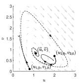
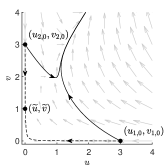
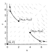
Figure 5: Example trajectories for two compartment systems where diffusion alters the steady state and leads to bounded (left panel) and unbounded (middle and right panel) solutions. The solid and dashed lines show the evolution of the species concentration in each compartment with and without diffusion, respectively. The gray arrows represent the vector field $(f,g)$ given by (34), (36), and (37) for the left, middle, and right panels, respectively. For complete details on simulations see Appendix B.1.

The second example of a strongly mutualistic population has the following reactions [14]

(36) $$f(u,v) \begin{aligned} =u(a_{1}-b_{1}u+c_{1}v)\end{aligned}$$

$$g(u,v) =v(a_{2}+b_{2}u-c_{2}v)$$

where $a_{1},a_{2}\in\mathbb{R}$ and $b_{1},b_{2},c_{1},c_{2}\in\mathbb{R_{+}}$. Here $a_{1}$ and $a_{2}$ represent growth or death rates of each species, $c_{1}$ and $b_{2}$ represent the positive mutual interaction between the two species, and the $b_{1}$ and $c_{2}$ represent growth limitations a species exerts on itself [21]. For strong mutualism we require $b_{2}c_{1}>b_{1}c_{2}.$ For some initial conditions the reaction-only system approaches a stable steady state while the spatially continuous RD system has unbounded solutions (see Proposition 1.1 and Theorem 1.2 in [14]). A LLF does not exist for this system (see Appendix B.3 for proof) which suggests the discretized RD system becomes unbounded. Numerical simulations confirm this result (Figure 5, middle panel).

The third and final example we will discuss was first introduced by [26]. The reactions are given as

(37) $$f(u,v) =uv(u-v)(u+1)-\delta u$$

$$g(u,v) =uv(v-u)(v+1)-\delta v$$

where $\delta$ is a positive constant. Again, these reactions satisfy the stated requirements in Section 2 since $f$ and $g$ are continuously differentiable and $f(0,v),g(u,0)\geq 0$. This system has a single steady state at the origin and a corresponding global Lyapunov function,

$$V(u,v)=(u+1)^{2}(v+1)^{2}.$$

This existence of this Lyapunov function proves that the steady state in the reaction-only system is globally stable.

For this system the conditions of Corollary 4.2 are satisfied and therefore an LLF does not exist (see Appendix B.3). Again however, this does not imply that the system is unbounded. Simulations of the two compartment system suggest that the system becomes unbounded as $t\rightarrow\infty$ (Figure 5, right panel), and in Appendix B.4 we prove this result for small $\delta$.

5 Discussion

We have defined a class of spatially discretized RD systems with a uniform boundedness property. We looked specifically at systems with two species reacting and diffusing on a 1D domain with homogeneous Neumann boundary conditions and guaranteed positivity of solutions. This RD system must additionally have a Lyapunov-like function (LLF) as described by Definition 2.2. Under these conditions, we are guaranteed that the total concentration of species in the system is bounded for all time. Notably, the existence of a LLF for a system only depends on the reactions, and is therefore independent of the domain size and diffusion rates of the two species in the system.

The results presented here are generalizable to systems with reaction parameters (i.e., parameters within the functions $f$ and $g$) and diffusion parameters (i.e., $d$ and $\gamma$) that vary across space. This generalization allows us to consider a broader range of systems. For example, parameter values could follow spatial gradients or the diffusion rate between two compartments could be altered to represent a physical barrier, such as a membrane. In a system with spatially varying reaction parameters, each individual compartment would have its own parameter set. For example, in (34) the reactions occurring in compartment $i$ would have parameters $a_{i}$ and $b_{i}$. If an LLF exists that satisfies (P1) in each spatial compartment, then our results can be generalized to prove that the system is bounded. To allow diffusion to vary across space, we would define a diffusion value of $u$ and $v$ across each edge in the system. The result of this change would cause the flux effect-terms given by (15) and (16) to depend on these edge-dependent diffusion values. In principle, the same logic in the proofs would hold, where the bounds obtained would now depend on the maximum and minimum values of the diffusion parameters. Rigorously proving these result is a topic of future research.

Using a LLF to prove boundedness provides a method for examining any mathematical description of a biological system. For example, biochemical dynamics can be described mathematically using mass-action kinetics [25], Hill Functions [10], and Michaelis-Menten Kinetics [13]. We specifically showed how the results can be applied to show boundedness in a system with mass-action kinetics (see first example Section 4.2). However, for many biological systems it might be challenging to find a suitable LLF. One solution to this challenge is to leverage computational work that has been done to find Lyapunov functions [11]. As shown in Corollary 4.1, a global Lyapunov function for the reactions might satisfy the requirements for a LLF. In cases where a global Lyapunov function does not lead to a suitable LLF, it might be possible to prove an LLF does not exist (see third example in Section 4.2). This suggests the system has the potential to become unbounded.

A natural future question regarding this work is whether a system that has a LLF remains bounded in the continuum limit. Here, the bound obtained depends on the number of spatial compartments and, therefore, the question of what occurs in the continuum limit is not yet answered. Additionally, the conditions for boundedness of one type of system (i.e., the discretized or continuous system) do not satisfy the conditions to guarantee boundedness of the other system (see [17] for conditions for the continuous system). Research looking at the continuous system with Dirichlet boundary conditions has found examples of systems that are bounded with respect to the $L^{1}$ norm but blow up with respect to the $L^{\infty}$ norm [23]. However, to the best of the author’s knowledge, no examples of this type have been found for systems with positive solutions and homogeneous Neumann boundary conditions. This suggests that boundedness for the class of RD systems discussed in the paper might be preserved in the continuum limit.

One motivation of this study was to find a class of RD systems that could be studied using systems biology approaches. When considering the discretized system it becomes feasible to apply existing systems biology tools, such as stoichiometric network analysis [2, 20, 9] and chemical reaction network theory [5, 3, 4], to study spatially heterogeneous systems or systems with bounded diffusion-driven instabilities. We have shown that the results presented here can be applied to this type of system (see first example in Section 4.2). In the future we hope to use systems biology tools to study how spatial features influence system properties (e.g., how does altering the diffusion ratio between two species affect the the space of possible reactive fluxes under steady-state conditions). Ultimately, the results presented here will help us study diffusion-driven instabilities in complex biochemical systems with variable diffusion and reaction rates.

Appendix A Proofs for the secondary properties of the LLF

In this section we will prove Corollary 2.1 and 2.3, which guarantee a LLF, $W:\mathbb{R}_{\geq 0}^{2}\rightarrow\mathbb{R}_{\geq 0}$, has the additional properties given by (C1)–(C5).

Proof A.1 (Proof of Corollary 2.1 (C1)).

Pick $L_{1}$ and $L_{2}$ such that $L_{2}>L_{1}>0$. Using (P2), we have that

$$M_{u}^{(L_{1})} =\max_{\|(u,v)\|=L_{1}}\partial_{u}W(u,v)$$

$$=\max_{v\in[0,L_{1}]}\partial_{u}W(L_{1}-v,v)$$

$$<\max_{u\in[0,L_{1}]}\partial_{u}W(L_{2}-v,v)$$

$$\leq\max_{u\in[0,L_{2}]}\partial_{u}W(L_{2}-v,v)=M_{u}^{(L_{2})}.$$

Here, the first inequality holds because $L_{2}>L_{1}$ and $\partial_{uu}W>0$. The second inequality holds because we are taking the maximum over a larger region. This result proves that $M_{u}^{(L)}$ is monotonically increasing. The result for $M_{v}^{(L)}$ follows analogously.

Proof A.2 (Proof of Corollary 2.1 (C2)).

By (P3) we know $W(u,0)\rightarrow\infty$ as $u\rightarrow\infty$. It follows that there exists a constant $\underline{u}$ such that $W(\underline{u},0)>W(0,0).$ Using the Mean Value Theorem and (P2), we have that $\partial_{u}W(\underline{u},0)>0.$ Therefore, by (P2), $\partial_{u}W(u,v)>0$ for all $v\geq 0$ and $u\geq\underline{u}$. The same logic can be used to prove there exists a constant $\underline{v}$ such that $\partial_{v}W(u,v)>0$ for all $v\geq\text{$\underline{v}$}$ and $u\geq 0$.

Proof A.3 (Proof of Corollary 2.1 (C3)).

Define

$$\hat{M}:=\max_{\|(u,v)\|\leq\text{$\underline{u}+\underline{v}$}}W(u,v).$$

By (P3) there exist constants $\widetilde{u},\widetilde{v}\in\mathbb{R}_{\geq 0}$ such that

(38) $$\min_{v\in[0,\underline{v}]}W(u,v) >\hat{M} \text{for }u\geq\widetilde{u}$$

$$\min_{u\in[0,\underline{u}]}W(u,v) >\hat{M} \text{for }v\geq\widetilde{v}.$$

Note that by definition $\widetilde{u}>\underline{u}+\underline{v}$ and $\widetilde{v}>\underline{u}+\underline{v}$.

Let $K:=\max\{\underline{K},\widetilde{u}+\widetilde{v}$} and recall that that $M^{(K)}=\max_{\|(u,v)\|=K}W(u,v)$. If $\|(u,v)\|=K$, then either $u\geq\widetilde{u}$ or $v\geq\widetilde{v}.$ We will show that $M^{(K)}>\hat{M}$ for $u\geq\widetilde{u}$, and the result for $v\geq\widetilde{v}$ follows analogously. If $u\geq\widetilde{u}$ and $v\leq\underline{v}$ then using (38) we have that $W(u,v)>\hat{M}$. If instead, $v>\underline{v}$, then $\partial_{v}W$ is positive and $W(u,v)>W(u,\underline{v})>\hat{M}$. Thus, if $\|(u,v)\|=K$ then $W(u,v)>\hat{M}$, and therefore $M^{(K)}>\hat{M}$.

Next pick $L<K$, and we will prove the claim in the corollary that $M^{(L)}<M^{(K)}.$ If $L\leq\underline{u}+\underline{v}$ we immediately have that $M^{(L)}\leq\hat{M}<M^{(K)}$. Alternatively, if $L>\underline{u}+\underline{v}$, we have that

$$M^{(L)} =\max_{\|(u,v)\|=L}W(u,v)=\max\left\{\max_{u\in[0,\underline{u}]}W(u,L-u),\max_{v\in[0,L-\underline{u}]}W(L-v,v)\right\}$$

$$<\max\left\{\max_{u\in[0,\underline{u}]}W(u,K-u),\max_{v\in[0,L-\underline{u}]}W(K-v,v)\right\}$$

$$\leq\max\left\{\max_{u\in[0,\underline{u}]}W(u,K-u),\max_{v\in[0,K-\underline{u}]}W(K-v,v)\right\}$$

$$=\max_{\|(u,v)\|=K}W(u,v)$$

$$=M^{(K)}.$$

In this calculation we are breaking apart the the line $\|(u,v)\|=L$ into two regions. In the region where $u\in[0,\underline{u}]$ we are guaranteed that $v>\underline{v}$ and thus, $\partial_{v}W>0$. In the other region where $v\in[0,L-\underline{u}]$ we are guaranteed that $u>\underline{u}$ and thus $\partial_{u}W>0.$ This leads to the first inequality. The second inequality follows because we are taking the maximum over a larger region. Note that by definition $K\geq\text{$\underline{K}$}$, $\underline{u}$, $\underline{v}$.

Proof A.4 (Proof of Corollary 2.3).

We will show the proof for (C4). The proof for (C5) follows analogously. Recall that

(39) $$M_{u}^{(\infty)}(v)=\lim_{u\rightarrow\infty}\partial_{u}W(u,v).$$

By (P2), $\partial_{uu}W>0$ and, therefore, $\partial_{u}W(u,v)$ is monotonically increasing with respect to $u$. This means that for a given $v$ the limit given by (39) either converges and exists or diverges to infinity. Furthermore, since $\partial_{uv}W(u,v)\geq 0$ we know that $M_{u}^{(\infty)}(v)$ must be monotonically non-decreasing with respect to $v$. Note that if for any $v\in[0,\infty)$, $M_{u}^{(\infty)}(v)=\infty$, then by (P5), $M_{u}^{(\infty)}(v)=\infty$ for all $v$, and the conclusions of the corollary follow. Therefore, in the remainder of the proof we will assume that $M_{u}^{(\infty)}(v)$ is finite for all $v\in[0,\infty).$ By (C2), we then have that $M_{u}^{(\infty)}(v)>0$.

First, we will show that $h(v):=\lim_{u\rightarrow\infty}\partial_{uv}W(u,v)=0$. By (P2) and (P5) we know $h(v)$ exists and is non-negative. This implies that there exists a constant $U>0$ such that if $u>U$ then $\partial_{uv}W(u,v)>h(v)/2$. We then have that

$$\int_{U}^{u}\partial_{uv}W(\widetilde{u},v)d\widetilde{u} \geq\int_{U}^{u}\frac{h(v)}{2}d\widetilde{u}$$

(40) $$\implies\partial_{v}W \geq\frac{h(v)}{2}u+C$$

where $C$ is a constant. Note that $\limsup_{u\rightarrow\infty}\partial_{v}W$ must be bounded for any $v\in[0,\infty)$ since

$$\sup_{u\geq\text{$\underline{u}$}}\left|\frac{\partial_{v}W(u,v)}{\partial_{u}W(u,v)}\right|\geq\limsup_{u\rightarrow\infty}\left|\frac{\partial_{v}W(u,v)}{\partial_{u}W(u,v)}\right|=\frac{\limsup_{u\rightarrow\infty}\left|\partial_{v}W(u,v)\right|}{M_{u}^{(\infty)}(v)}.$$

and by (P4) the supremum is finite. Taking the limsup of both sides of (40) as $u\rightarrow\infty$ shows that this bound would not hold if $h(v)>0$. Therefore, $h(v)=0$ for all $v\in[0,\infty).$

Our next goal is to show that $h^{\prime}(v)=\lim_{u\rightarrow\infty}\partial_{uv}W(u,v)$ for all $v\in[0,\infty)$. Notice that this relation can be rewritten as

$$\lim_{h\rightarrow 0}\lim_{u\rightarrow\infty}F(u,v,h)=\lim_{u\rightarrow\infty}\lim_{h\rightarrow 0}F(u,v,h)$$

where

$$F(u,v,h)=\frac{\partial_{u}W(u,v+h)-\partial_{u}W(u,v)}{h}.$$

Thus, we need to show that the limits are interchangeable.

Since $\partial_{u}W(u,v)$ converges pointwise to $g(v)$ as $u\rightarrow\infty$ and $\partial_{u}W(u,v)$ is monotonically increasing with respect to $u$, by Dini’s Monotone Convergence Theorem $\partial_{u}W(u,v)$ converges uniformly to $g(v)$ for $v\in[0,L]$ where $L$ is an arbitrary constant. Therefore $\lim_{u\rightarrow\infty}F(u,v,h)$ exists and converges uniformly. We furthermore know that the $\lim_{h\rightarrow 0}F(u,v,h)$ exists and converges pointwise. Thus, by the Moore-Osgood Theorem, the limits are interchangeable and the resulting values are equal.

In conclusion, we have that

$$\frac{d}{dv}M_{u}^{(\infty)}(v) =\frac{d}{dv}\lim_{u\rightarrow\infty}\partial_{u}W(u,v)=\lim_{u\rightarrow\infty}\partial_{uv}W(u,v)=0$$

Thus, for all $v\in[0,L]$, $M_{u}^{(\infty)}(v)$ is constant. Let $M_{u}^{(\infty)}:=M_{u}^{(\infty)}(v)$ and note that the upper bound $L$ was arbitrary and therefore we have that this equality holds for all $v\in[0,\infty)$.General rules for determining whether an LLF exists: Proofs

Below are the proofs for Corollary 4.1 and 4.2 in the paper.

Proof A.5 (Proof of Corollary 4.1).

We can immediately show that $W$ satisfies (P4) since

$$\sup_{v\geq\underline{v}}\left|\frac{\partial_{u}W(u,v)}{\partial_{v}W(u,v)}\right| \leq\frac{w_{1}^{\prime}(u)}{w_{2}^{\prime}(v)}\leq\frac{w_{1}^{\prime}(u)}{w_{2}^{\prime}(\underline{v})}<\infty$$

$$\sup_{u\geq\underline{u}}\left|\frac{\partial_{v}W(u,v)}{\partial_{u}W(u,v)}\right| \leq\frac{w_{2}^{\prime}(v)}{w_{1}^{\prime}(u)}\leq\frac{w_{2}^{\prime}(v)}{w_{1}^{\prime}(\underline{u})}<\infty.$$

Additionally (P5) is satisfied since

$$\lim_{u\rightarrow\infty}\partial_{u}W(u,v) =\lim_{u\rightarrow\infty}w^{\prime}_{1}(u)=C_{1}$$

$$\lim_{v\rightarrow\infty}\partial_{v}H(u,v) =\lim_{v\rightarrow\infty}w_{2}^{\prime}(v)=C_{2}$$

$$\partial_{uv}W(u,v) =0$$

where, due to (P2), $C_{1}$ and $C_{2}$ are constants or infinite.

Proof A.6 (Proof of Corollary 4.2).

We will show that if there exists a $v$ such that (31) is satisfied, then no LLF exists. The result for any $u$ and (32) follows analogously. Suppose there exists a LLF for the system. By (P1), there exists a $\underline{K}$ such that, if $\|(u,v)\|>\underline{K}$, then

(41) $$\left(\nabla W\right)(f,g)^{T} =\partial_{u}W(u,v)f(u,v)+\partial_{v}W(u,v)g(u,v)\leq 0$$

Pick $v>0$ and consider what happens in the limit as $u\rightarrow\infty$. By (P1), (C2), and (31), there exists $\widetilde{u}$ such that if $u>\widetilde{u}$ then $u>\underline{K}$, $\partial_{u}W>0$, and $f(u,v)>0$. We therefore have that for $u\geq\widetilde{u}$,

$$\frac{\partial_{v}W(u,v)}{\partial_{u}W(u,v)}\begin{cases}\leq-\frac{f(u,v)}{g(u,v)}<0&\text{if }g(u,v)>0\\ \geq-\frac{f(u,v)}{g(u,v)}>0&\text{if }g(u,v)<0.\end{cases}$$

Note that since $f>0$ and $\partial_{u}W>0$, in order for (41) to hold, $g\neq 0$. This set of inequalities implies that

$$\left|\frac{\partial_{v}W(u,v)}{\partial_{u}W(u,v)}\right|\geq\left|\frac{f(u,v)}{g(u,v)}\right|.$$

Note that, in the limit as $u\rightarrow\infty$, $\left|f(u,v)/g(u,v)\right|=\infty$ and, therefore

$$\sup_{u\geq\text{$\underline{u}$}}\left|\frac{\partial_{v}W(u,v)}{\partial_{u}W(u,v)}\right|=\infty.$$

This final equation gives us a contradiction to (P4). Therefore, no LLF exists for the reactions.

Appendix B Example Systems

Below we provide details on the simulations and LLF results discussed in Section 4.2.

B.1 Parameters for performing simulations

Here we give the parameters used to perform the simulations shown in Figure 5. For simulations with diffusion the system given by (2) was used where $n=2$. In the simulation shown in the left panel, $f$ and $g$ are given by (34) where $a=0.1$, $b=1$, $\gamma=150$, $d=30$, $(u_{1,0},v_{1,0})=(0.8,0.1)$ and $(u_{2,0},v_{2,0})=(2.0,0.7)$. For the simulation shown in the middle panel, $f$ and $g$ are given by (36) where $a_{1}=-1$, $a_{2}=1$, $b_{1}=1$, $b_{2}=2$, $c_{1}=1$, $c_{2}=1$, $\gamma=1$, $d=1$, $(u_{1,0},v_{1,0})=(3,0.001)$ and $(u_{2,0},v_{2,0})=(0.001,3)$. For the simulation shown in the right panel, $f$ and $g$ are given by (37) where $d=1$, $\gamma=1$, $\delta=10$, $u_{1,0}=v_{2,0}=2$, and $u_{2,0}=v_{1,0}=4$.

B.2 Existence of Lyapunov-like function for first example

In this section we prove that the LLF given by (35) has the properties (P1)–(P5) given in Section 2.1. We will go through each property individually:

1. We will show that for large enough $\|(u,v)\|$, $\left(\nabla W\right)(f,g)^{T}$ is negative. We have that

   $$\left(\nabla W\right)(f,g)^{T}=\left(1-\frac{c}{(u+1)^{2}}\right)(a-u+u^{2}v)+\left(2-\frac{1}{(1+v)^{2}}\right)(b-u^{2}v).$$

   Combining the terms and using $N(u,v)$ to represent the numerator we can write this equation as follows:

   $$\left(\nabla W\right)(f,g)^{T}=\frac{N(u,v)}{(1+u)^{2}(1+v)^{2}}$$

   We will show that there exists a value $\underline{K}$ such that if $\|(u,v)\|>\underline{K}$, then $N(u,v)<0$. To do this we will find threshold values for $u$ and $v$ separately.

   1. Let’s first consider $u$. After some algebraic manipulates, we rewrite $N(u,v)$ as

      $$N(u,v) =(1+u^{2})(a+b-u)+u(2a+2b+c-2u)$$

      $$+(2v+2u^{2}v+v^{2}+u^{2}v^{2})(a+2b-u)$$

      $$+(2uv+uv^{2})(2a+4b+c-2u)$$

      $$-ac-2acv-cu^{2}v-acv^{2}-(2c+2)u^{2}v^{2}$$

      $$-4u^{3}v^{2}-2u^{4}v^{2}-u^{2}v^{3}-cu^{2}v^{3}-2u^{3}v^{3}-u^{4}v^{3}.$$

      This equation is negative if $u>\widetilde{u}:=a+2b+\frac{c}{2}$.

   2. Let’s next consider $v$ and write $N(u,v)$ as follows

      $$N(u,v) =v^{2}(a+2b-\frac{ac}{2})+u^{2}v^{3}(a+2b-\frac{c}{2})+(a+b-2acv)$$

      $$+u(2a+2b+c-2v)+u^{2}(a+b-cv)+v(3a+6b+\frac{c}{2}-\frac{ac}{2}v)$$

      $$+uv(4a+8b+2c-v)+u^{2}v^{2}(a+2b-v)+2u^{2}v(a+2b-cv)$$

      $$-ac-u-2u^{2}-u^{3}-4u^{2}v-2u^{3}v-(a+2b+\frac{c}{2})v(uv-1)^{2}$$

      $$-4u^{2}v^{2}-5u^{3}v^{2}-2u^{4}v^{2}-2u^{3}v^{3}-u^{4}v^{3}.$$

      This equation is negative if $c>\max\{(2a+4b)/a,2a+4b\}$ and

      $$v >\widetilde{v}:=\max\left\{4a+8b+2c,\frac{6a+12b+c}{ac},\frac{a+2b}{c}\right\}$$

   Let $\underline{K}:=\widetilde{u}+\widetilde{v}$. If $\|(u,v)\|>\underline{K}$ then either $u>\widetilde{u}$ or $v>\widetilde{v}$ and, therefore, $\left(\nabla W\right)^{T}(f,g)<0$.

2. Taking the second derivatives of $W$ gives us:

   $$\partial_{uu}W =\frac{2c}{(u+1)^{3}}>0$$

   $$\partial_{vv}W =\frac{2}{(v+1)^{3}}>0$$

   $$\partial_{uv}W =0.$$

   Thus, the desired inequalities are satisfied.

3. We have that,

   $$W(u,v)=\|(u,v)\|+v+\frac{c}{u+1}+\frac{1}{v+1}\geq\|(u,v)\|.$$

   Thus, as $\|(u,v)\|\rightarrow\infty$, $W(u,v)\rightarrow\infty$.

4. Note, that for this system $\partial_{u}W>0$ if $u\geq c$ and $\partial_{v}W>0$ if $v\geq 0.$ Therefore, we set $\underline{u}=c$ and $\underline{v}=0$. For an arbitrary $u>0$, we have that

   $$\sup_{v\geq\underline{v}}\left|\frac{\partial_{u}W(u,v)}{\partial_{v}W(u,v)}\right|=\sup_{v\geq 0}\frac{\left|1-\frac{c}{(u+1)^{2}}\right|}{2-\frac{1}{(v+1)^{2}}}\leq\left|1-\frac{c}{(u+1)^{2}}\right|<\infty$$

   and for an arbitrary $v>0$, we have that

   $$\sup_{u\geq\underline{u}}\left|\frac{\partial_{v}W(u,v)}{\partial_{u}W(u,v)}\right|=\sup_{u\geq c}\frac{2-\frac{1}{(v+1)^{2}}}{1-\frac{c}{(u+1)^{2}}}\leq\frac{2-\frac{1}{(v+1)^{2}}}{1-\frac{c}{(c+1)^{2}}}<\infty.$$

   Thus, the specified supremums are finite.

5. Taking the limits specified in the property gives us

   $$\lim_{u\rightarrow\infty}\partial_{u}W(u,v) =\lim_{u\rightarrow\infty}\left(1-\frac{c}{(u+1)^{2}}\right)=1$$

   $$\lim_{v\rightarrow\infty}\partial_{v}W(u,v) =\lim_{v\rightarrow\infty}\left(2-\frac{1}{(v+1)^{2}}\right)=2$$

   $$\lim_{u\rightarrow\infty}\partial_{uv}W(u,v) =\lim_{v\rightarrow\infty}\partial_{uv}W(u,v)=0.$$

   Therefore, all the limits exist and are finite.

B.3 No Lyapunov-like function exists for unbounded examples

In this section we show that no LLF exists for the two unbounded example systems. We will first consider the system given by (36) and suppose an LLF does exist. By (P1) we have that there exists a $\underline{K}>0$ such that if $\|(u,v)\|\geq\underline{K}$ then

$$\partial_{u}W(u,v)(u(a_{1}-b_{1}u+c_{1}v))+\partial_{v}W(v(a_{2}+b_{2}u-c_{2}v))\leq 0.$$

Suppose $v=\frac{b_{2}}{c_{2}}u$ and $v\geq\underline{v}$, $u\geq\underline{u}$. We then have that $\partial_{u}W(u,v),\partial_{v}W(u,v)>0$ and

$$\partial_{u}W(u,v)\left(a_{1}u+\left(c_{1}\frac{b_{2}}{c_{2}}-b_{1}\right)u^{2}\right)+\partial_{v}W\left(a_{2}\frac{b_{2}}{c_{2}}u\right) \leq 0.$$

$$\implies a_{1}u+\left(c_{1}\frac{b_{2}}{c_{2}}-b_{1}\right)u^{2} \leq 0$$

Note that as $u\rightarrow\infty,$the quadratic term dominates and therefore we require that

$$c_{1}b_{2}-b_{1}c_{2}\leq 0.$$

However, recall that for the system to be strongly mutualistic we require that $b_{2}c_{1}>b_{1}c_{2}$ and therefore we have a contradiction. Therefore, no LLF exists for this system.

Next, we will use Corollary 4.2 to show that no LLF exists for the reactions given by (37). Suppose we fix a value of $v>0$ and consider what happens in the limit as $u\rightarrow\infty$. We have that at some point $u>v+1$ and $u>\delta/v-1.$ This leads to the follow inequalities

$$f(u,v) =uv(u-v)(u+1)-\delta u>0$$

$$g(u,v) =uv(v-u)(v+1)-\delta v<0$$

and we have that

$$\lim_{u\rightarrow\infty}\left|\frac{f(u,v)}{g(u,v)}\right|=\lim_{u\rightarrow\infty}\frac{uv(u-v)(u+1)-\delta u}{uv(u-v)(v+1)+\delta v}=\lim_{u\rightarrow\infty}\frac{(u+1)-\frac{\delta}{v(u-v)}}{(v+1)+\frac{\delta}{u(u-v)}}=\infty.$$

Thus, by Corollary 4.2 no LLF for the system exists.

B.4 Unboundedness of example system

In this section, we will show that the discretized RD system given by (2) with parameters $\gamma=1$, $d=1$, and $n=2$ and reactions given by (37) has the capacity to become unbounded. We will use symmetric initial conditions (i.e. $u_{1,0}=v_{2,0}$ and $u_{2,0}=v_{1,0}$). It follows that, due to the symmetry of the reactions, $u_{1}(t)=v_{2}(t)$ and $u_{2}(t)=v_{1}(t)$ for all $t>0$. Therefore, the system reduces to

$$\frac{du}{dt} =uv(u-v)(u+1)-\delta u+4(v-u)$$

(42) $$\frac{dv}{dt} =uv(v-u)(v+1)-\delta v+4(u-v)$$

$$u(0) =u_{0}$$

$$v(0) =v_{0}$$

where $u_{0}=u_{1,0}=v_{2,0}$ and $v_{0}=u_{2,0}=v_{1,0}.$ We can then calculate the concentration of species in each compartment as $u_{1}(t)=v_{2}(t)=u(t)$ and $v_{1}(t)=u_{2}(t)=v(t)$.

Let’s consider (42) and calculate how the difference between $u$ and $v$ evolves with time:

(43) $$(u-v)_{t} =uv(u-v)(u+v+2)+(8+\delta)(v-u)$$

$$=(u-v)h(u,v).$$

where

$$h(u,v):=uv(u+v+2)-(8+\delta),$$

Therefore if,

(44) $$u-v >0$$

$$h(u,v) >0$$

then $(u-v)_{t}>0$.

We will show that there exists a $\delta>0$ such that for arbitrarily small $\epsilon>0$, $dh/dt$ is positive along the curve

(45) $$h(u,v)=\epsilon.$$

Therefore, if the initial data satisfies (44) then these inequalities will be satisfied for all time.

We first solve (45) explicitly for $v$ to obtain the positive solution

(46) $$v=-1-\frac{1}{2}u+\sqrt{\frac{8+\delta+\epsilon}{u}+1+u+\frac{u^{2}}{4}}.$$

Note that this function is symmetric about the line $u=v$ and it is concave upwards (i.e., $d^{2}v/du^{2}>0$). We will show that there exists a constant $C$ such that, along the curve given by (45), $u+v\geq C>0$. Suppose it is not the case (i.e., $u+v<C$) and add $u$ to both sides of (46) to obtain

$$C>u+v=-1+\frac{1}{2}u+\sqrt{\frac{8+\delta+\epsilon}{u}+1+u+\frac{u^{2}}{4}}.$$

Using algebraic manipulations, we obtain the following inequality:

$$0 >(2+C)u^{2}-C(2+C)u+8+\delta+\epsilon.$$

The maximum value of $C$ which guarantees that no real solutions to this equation exist is given by the solution to $0=C^{3}+2C^{2}-32$. We will define $C$ as the one real root to this equation. We are then guaranteed that along the curve (45), $u+v\geq C$.

Next, we will assume $u-v>0$ and break up the curve given by (45) into two regions: $0<u-v\leq 1$ and $1<u-v$. For both these regions we will calculate $dh/dt$ along (45) and show that, under certain conditions, it is positive. We will further suppose that $\epsilon+\delta<1$.

Suppose $0<u-v\leq 1$. In order to show that $dh/dt$ is increasing along the curve, we will find a lower bound for the value of $u+v$ and translate that into an upper bound on the value of $uv$. Due to the positive second derivative and symmetry of (46), we know the maximum value of $u+v$ along the curve occurs when $v=u-1$. We will call this point $(u_{max},v_{max}).$ Note that $C\leq u_{max}+v_{max}=2u_{max}-1$, and therefore $u_{max}\geq(C+1)/2$. We will next calculate an upper bound on $u_{max}$. We have that

$$h(u_{max},v_{max}) =\epsilon$$

$$u_{max}v_{max}(u_{max}+v_{max}+2) =\epsilon+\delta+8$$

$$u_{max}(u_{max}-1)(2u_{max}+1) =\epsilon+\delta+8$$

$$u_{max}-1 =\frac{\epsilon+\delta+8}{u_{max}(2u_{max}+1)}$$

$$u_{max}-1 <\frac{9}{\frac{(C+1)}{2}(C+2)}=\frac{18}{(C+1)(C+2)}$$

$$u_{max} <\frac{18}{(C+1)(C+2)}+1$$

It then immediately follows that $v_{max}<\frac{18}{(C+1)(C+2)}.$ We then have that, along the curve given by (45)

$$uv=\frac{\epsilon+\delta+8}{u+v+2}>\frac{\epsilon+\delta+8}{u_{max}+v_{max}+2}>\frac{8}{\frac{36}{(C+1)(C+2)}+3}=:A.$$

Finally, we consider and bound the derivative of $h$ along the curve. Recall that $u+v>C$ and $\delta+\epsilon<1$. We have that along 45 when $0<u-v\leq 1$

$$\frac{dh(u,v)}{dt} =(u-v)^{2}(2+u+v)(4-uv)+2uv+\left(uv\right)^{2}(u-v)^{2}-\delta uv(4+3(u+v))$$

$$\geq(u-v)^{2}(4(2+u+v)-(8+\delta+\epsilon))+uv(2-\delta(4+3(u+v)))$$

$$\geq(u-v)^{2}(4C-1)+uv(2+2\delta-3\delta(u+v+2))$$

$$\geq uv(2+2\delta)-3\delta(8+\epsilon+\delta)$$

$$\geq A(2+2\delta)-27\delta$$

$$\geq 2A-(27-2A)\delta.$$

Thus, if $\delta<\frac{2A}{27-2A}$ then the derivative is increasing.

Suppose $u-v>1.$ The derivative of $h$ along the curve is bounded as follows:

$$\frac{dh(u,v)}{dt} =(u-v)^{2}(2+u+v)(4-uv)+2uv+\left(uv\right)^{2}(u-v)^{2}-\delta uv(4+3(u+v))$$

$$\geq(4(2+u+v)-(8+\delta+\epsilon))-\delta uv(4+3(u+v)))$$

$$\geq(4C-1)-\delta uv(-2+3(u+v+2)))$$

$$\geq(4C-1)+2\delta uv-3\delta(8+\epsilon+\delta)$$

$$\geq(4C-1)-3\delta(8+\epsilon+\delta)$$

$$\geq(4C-1)-27\delta$$

So the derivative is positive if $\delta<\frac{4C-1}{27}$.

Therefore, for small enough $\delta$, if the system satisfies (44) it will continue to do so for all time. Numerically, we determined that if $\delta\leq 0.13$ then the necessary conditions are satisfied.

Using (43) and assuming the initial data satisfies (44), we have that for small enough $\epsilon>0$.

$$(u-v)_{t} \geq\epsilon(u-v).$$

Using Grönwall’s inequality, we then have that

$$u(t)-v(t)\geq(u_{0}-v_{0})e^{\epsilon t}.$$

Therefore, since $v(t)\geq 0$, $u(t)\rightarrow\infty$ as $t\rightarrow\infty$. Note that analogously we could pick initial conditions where $v_{0}>u_{0}$ and $u_{0}v_{0}(u_{0}+v_{0}+2)>8+\delta$ and this would lead to a blow up of $v(t)$.

References

- [1] L. J. S. Allen, Persistence, extinction, and critical patch number for island populations, J. Math. Biol., 24 (1987), pp. 617–625.
- [2] B. L. Clarke, Stoichiometric network analysis, Cell Biophysics, 12 (1988), pp. 237–253.
- [3] G. Craciun and M. Feinberg, Multiple equilibria in complex chemical reaction networks: I. The injectivity property, SIAM J. Appl. Math, 65 (2005), pp. 1526–1546.
- [4] G. Craciun and M. Feinberg, Multiple equilibria in complex chemical reaction networks: II. The species-reaction graph, SIAM J. Appl. Math, 66 (2006), pp. 1321–1338.
- [5] M. Feinberg, Lectures on chemical reaction networks., Notes of lectures given at the Mathematics Research Center, University of Wisconsin, (1979), p. 49.
- [6] M. Fila and H. Ninomiya, Reaction versus diffusion: blow-up induced and inhibited by diffusivity, Russian Math. Surveys, 60 (2005), pp. 1217–1235.
- [7] W. B. Fitzgibbon, S. L. Hollis, and J. J. Morgan, Stability and Lyapunov functions for reaction-diffusion systems, SIAM J. Math. Anal., 28 (1997), pp. 595–610.
- [8] C. H. Flather and M. Bevers, Patchy reaction-diffusion and population abundance: The relative importance of habitat amount and arrangement, American Naturalist, 159 (2002), pp. 40–56.
- [9] E. P. Gianchandani, A. K. Chavali, and J. A. Papin, The application of flux balance analysis in systems biology, Wiley Interdisciplinary Reviews: Systems Biology and Medicine, 2 (2010), pp. 372–382.
- [10] S. Goutelle, M. Maurin, F. Rougier, X. Barbaut, L. Bourguignon, M. Ducher, and P. Maire, The Hill equation: a review of its capabilities in pharmacological modelling, Fundamental & Clinical Pharmacology, 22 (2008), pp. 633–648.
- [11] S. Hafstein and P. Giesl, Review on computational methods for Lyapunov functions, Discrete Contin. Dyn. Syst. Ser. B, 20 (2015), pp. 2291–2331.
- [12] S. L. Hollis, R. H. Martin, Jr., and M. Pierre, Global existence and boundedness in reaction-diffusion systems, SIAM J. Appl. Math, 18 (1987), pp. 744–761.
- [13] K. A. Johnson and R. S. Goody, The original Michaelis constant: Translation of the 1913 Michaelis-Menten paper, Biochemistry, 50 (2011), pp. 8264–8269.
- [14] Y. Lou, T. Nagylaki, and W. M. Ni, On diffusion-induced blowups in a mutualistic model, Nonlinear Anal., 45 (2001), pp. 329–342.
- [15] A. Marciniak-Czochra, G. Karch, K. Suzuki, and J. Zienkiewicz, Diffusion-driven blowup of nonnegative solutions to reaction-diffusion-ODE systems, Differential Integral Equations, 29 (2016), pp. 7–8.
- [16] L. Melkemi, A. Z. Mokrane, and A. Youkana, Boundedness and Large-Time Behavior Results for a Diffusive Epidemic Model, J. Appl. Math., (2007), p. 15.
- [17] J. Morgan, Boundedness and decay results for reaction-diffusion systems, SIAM J. Math. Anal., 21 (1990), pp. 1172–1189.
- [18] J. D. Murray, Mathematical Biology: I. An Introduction, Springer-Verlag New York, 3 ed., 2002.
- [19] J. D. Murray, Mathematical Biology: II. Spatial Models and Biomedial Applications, Springer-Verlag New York, 3 ed., 2003.
- [20] B. Palsson, Systems biology: properties of reconstructed networks, Cambridge and New York: Cambridge University Press, 2006.
- [21] C. V. Pao, Nonlinear Parabolic and Elliptic Equations, Springer US, 1993.
- [22] B. Perthame, Parabolic Equations in Biology, Springer, 2015.
- [23] M. Pierre, Global Existence in Reaction-Diffusion Systems with Control of Mass: A Survey, Milan J. Math., 78 (2010), pp. 417–455.
- [24] J. Schnakenberg, Simple chemical reaction systems with limit cycle behaviour, J. Theoret. Biol., 81 (1979), pp. 389–400.
- [25] E. O. Voit, H. A. Martens, and S. W. Omholt, 150 Years of the Mass Action Law, PLoS Computational Biology, 11 (2015), p. e1004012.
- [26] H. F. Weinberger, An example of blowup produced by equal diffusions, J. Differential Equations, 154 (1999), pp. 225–237.
- [27] J. M. Wentz, A. R. Mendenhall, and D. M. Bortz, Pattern formation in the longevity-related expression of heat shock protein-16.2 in Caenorhabditis elegans, Bull. Math. Bio., 80 (2018), pp. 2669–2697.
- [28] A. Zecchin, P. C. Stapor, J. Goveia, and P. Carmeliet, Metabolic pathway compartmentalization: An underappreciated opportunity?, aug 2015.