Drastic enhancement of the thermal Hall angle in a $d$-wave superconductor

Abstract

A drastic enhancement of the thermal Hall angle in $d$-wave superconductors was observed experimentally in a cuprate superconductor and in CeCoIn₅ at low temperatures and very weak magnetic field [Phys. Rev. Lett. 86, 890 (2001); Phys. Rev. B 72, 214515 (2005)]. However, to the best of our knowledge, its microscopic calculation has not been performed yet. To study this microscopically, we derive the thermal Hall coefficient in extreme type-II superconductors with an isolated pinned vortex based on the augmented quasiclassical equations of superconductivity with the Lorentz force. Using it, we can confirm that the quasiparticle relaxation time and the thermal Hall angle are enhanced in $d$-wave superconductors without impurities of the resonant scattering because quasiparticles around the gap nodes which become dominant near zero temperature are restricted to the momentum in a specific orientation. This enhancement of the thermal Hall angle may also be observed in other nodal superconductors with large magnetic-penetration depth.

I Introduction

It was observed experimentally that the thermal conductivity and the thermal Hall angle are greatly enhanced in the superconducting states of cuprates Cohn ; Krishana95 ; Zeini99 ; Krishana99 ; Zhang00 ; Ocana ; Zhang01 ; Zeini01 and CeCoIn₅ Kasahara . These materials are regarded as $d$-wave superconductors, and their thermal Hall conductivity is also consistent with the scaling relation for a $d$-wave pairing based on the Bogoliubov–de Gennes equation Simon . Hirschfeld et al. also calculated the longitudinal thermal conductivity in a $d$-wave superconductor, including the effect of antiferromagnetic spin fluctuations within the random phase approximation (RPA), and studied the large peak structure of the longitudinal thermal conductivity in YBa₂Cu₃O_7-δ (YBCO) Hirschfeld96 . The enhancement of the thermal Hall angle has been explained to originate from the enhancement of the quasiparticle mean free path Zhang01 ; Kasahara . However, to the best of our knowledge, its microscopic calculation has not been carried out yet. Therefore, the origin of the enhancement of the quasiparticle mean free path needs to be clarified using a fully microscopic treatment. The purpose of this present paper is to develop a theoretical formalism for investigating the thermal Hall conductivity microscopically within the quasiclassical theory and to study this drastic enhancement of the thermal Hall angle in the superconducting states of YBCO and CeCoIn₅.

Numerous theoretical studies have been carried out, such as on the longitudinal component of the thermal conductivities in both conventional ($s$-wave) Bardeen ; Graf ; Adachi and unconventional superconductors Hirschfeld96 ; Schmitt ; Hirschfeld88 ; Graf ; Kubert ; Franz ; Vekhter ; Vorontsov ; Adachi ; Hara ; Kobayashi and the spontaneous thermal Hall conductivity due to the intrinsic Read ; Nomura ; Sumiyoshi ; Imai16 ; Yoshioka and extrinsic Yip ; Yilmaz ; Ngampruetikorn ; Ngampruetikorn20 mechanisms in chiral superconductors. On the other hand, several studies have been carried out on the thermal Hall conductivity in $d$-wave superconductors, in terms of the cross section of quasiparticle scattering from a single vortex Durst , due to the Berry phase acquired by a quasiparticle in the vortex lattice state Vafek01 ; Cvetkovic ; Murray ; Vafek15 , based on the Kubo formula approach and taking into account the Doppler shift effect Shahzamanian . The thermal Hall conductivity due to the Lorentz force in type-II superconductors is not fully understood, this may be because the Lorentz force is missing from the quasiclassical Eilenberger equations Eilenberger , which is a powerful tool for investigating inhomogeneous and nonequilibrium superconductors microscopically Eschrig . More precisely, the component of the magnetic Lorentz force balanced with the Hall electric field and/or force induced by a transverse temperature gradient may be missing from the standard Eilenberger equations, since there is the component of the magnetic Lorentz force balanced with the hydrodynamic force in the Ginzburg–Landau equations Kato16 .

Here we derive the thermal Hall coefficient in extreme type-II superconductors with an isolated pinned vortex, based on the augmented quasiclassical equations of superconductivity with the Lorentz force in the Keldysh formalism Kita01 by incorporating a next-to-leading-order contribution in the expansion of the Gor’kov equations Gor'kov ; Gor'kov2 in terms of the quasiclassical parameter $\delta\equiv 1/k_{\rm F}\xi_{0}(0)$, where $k_{\rm F}$ and $\xi_{0}(0)$ denote the Fermi wave number and the coherence length at zero temperature, respectively. The calculations of linear responses based on the augmented equations obtained from this derivation Kita01 have not been performed yet, as far as we know, except for the flux-flow Hall effect Arahata . In extreme type-II superconductors with an isolated pinned vortex, the thermal conductivity is dominated by the contribution from quasiparticles outside the core. Thus, we consider the contribution of the Doppler shifted quasiparticles due to the circulating supercurrent around the core (i.e., the Volovik effect) Kubert ; Volovik ; Kopnin and neglect that of the Andreev-reflected quasiparticles in the core Dahm ; Nagai . The newly derived expression for the thermal conductivity is an extension of the expression proposed by Graf et al. Graf and can also describe the thermal Hall effect in both fully gapped and nodal superconductors. Based on this formalism, we calculate the thermal conductivity and the thermal Hall angle in $d$-wave superconductors and address the enhancement of $\lim_{H\to 0}\tan\theta_{\rm H}/H$ at low temperatures in YBCO and CeCoIn₅ measured by Zhang et al. in Ref. Zhang01, and by Kasahara et al. in Ref. Kasahara, , where $\tan\theta_{\rm H}$ and $H$ denote the thermal Hall angle and the external magnetic field, respectively. It is also imperative to consider impurity scattering close to the unitarity limit to explain the experimental results on the longitudinal thermal conductivity in heavy-fermion superconductors and Zn-doped YBCO Coffey ; Hirschfeld96 ; Schmitt ; Hirschfeld88 . Thus, we also study the impurity effect on the thermal Hall conductivity and the thermal Hall angle in a $d$-wave superconductor, using the impurity self-energy by $t$-matrix approximation Hirschfeld96 ; Schmitt ; Hirschfeld88 ; Graf ; Vorontsov ; Kato00 .

This paper is organized as follows. In Sec. II, we present the augmented quasiclassical equations of superconductivity with the Lorentz force in the Keldysh formalism. In Sec. III, we derive the thermal Hall coefficient in extreme type-II superconductors with an isolated pinned vortex based on the augmented quasiclassical equations of superconductivity with the Lorentz force and the linear response theory. In Sec. IV, we present numerical results for the thermal Hall effect in $d$-wave superconductors. In Sec. V, we provide concluding remarks.

II Augmented Quasiclassical Equations

We consider type-II superconductors with pinned vortices and neglect the pair-potential-gradient force Ohuchi ; Masaki17 ; Masaki18 and the pressure difference arising from the slope in the density of states (DOS) Ueki18 , which only contribute to the vortex-core charging in this case, since the charge in a pinned vortex does not contribute to thermal conductivity. For simplicity, we also restrict ourselves to the spin-singlet pairing without spin paramagnetism. Then the quasiclassical equations of superconductivity with the Lorentz force are given in the Keldysh formalism by Kita01

$$\left[\varepsilon\check{\tau}_{3}-\check{\Delta}-\check{\sigma},\check{g}\right]_{\circ}+{i}\hbar{\bm{v}}_{\rm F}\cdot{\bm{\partial}}\check{g}$$

$$+\frac{{i}\hbar}{2}\left[e{\bm{v}}_{\rm F}\cdot{\bm{E}}\frac{\partial}{\partial\varepsilon}+e\left({\bm{v}}_{\rm F}\times{\bm{B}}\right)\cdot\frac{\partial}{\partial{\bm{p}}_{\rm F}}\right]\left\{\check{\tau}_{3},\check{g}\right\}=\check{0},$$ (1)

where $e<0$ is the electron charge, ${\bm{E}}$ is the electric field, ${\bm{B}}$ is the magnetic field, $\varepsilon$ is the excitation energy, ${\bm{v}}_{\rm F}$ is the Fermi velocity, and ${\bm{p}}_{\rm F}$ is the Fermi momentum. The Green’s functions $\check{g}$, the pair potential $\check{\Delta}$, and the Born-type impurity self-energy $\check{\sigma}$ can be written as

$$\check{g}=\begin{bmatrix}\hat{g}^{\rm R}&\hat{g}^{\rm K}\\ \hat{0}&\hat{g}^{\rm A}\end{bmatrix},\ \ \ \check{\Delta}=\begin{bmatrix}\hat{\Delta}&\hat{0}\\ \hat{0}&\hat{\Delta}\end{bmatrix},$$

$$\check{\sigma}=-\frac{{i}\hbar}{2\tau}\langle\check{g}\rangle_{\rm F}=\begin{bmatrix}\hat{\sigma}^{\rm R}&\hat{\sigma}^{\rm K}\\ \hat{0}&\hat{\sigma}^{\rm A}\end{bmatrix},$$ (2)

where $\tau$ is the relaxation time and $\langle\cdots\rangle_{\rm F}$ denotes the Fermi surface average with $\langle 1\rangle_{\rm F}=1$. This Born-type impurity self-energy will later be rewritten to the impurity self-energy by the $t$-matrix approximation Graf ; Vorontsov ; Kato00 . The $2\times 2$ retarded and Keldysh Green’s functions and the $2\times 2$ pair potential can be written as

$$\hat{g}^{\rm R,A}=\begin{bmatrix}g^{\rm R,A}&-{i}f^{\rm R,A}\\ {i}\bar{f}^{\rm R,A}&-\bar{g}^{\rm R,A}\end{bmatrix},\ \ \ \hat{g}^{\rm K}=\begin{bmatrix}g^{\rm K}&-{i}f^{\rm K}\\ -{i}\bar{f}^{\rm K}&\bar{g}^{\rm K}\end{bmatrix},$$

$$\hat{\Delta}=\begin{bmatrix}0&-\Delta\phi\\ \Delta^{*}\phi^{*}&0\end{bmatrix},$$ (3)

where the barred function in the Keldysh formalism is defined generally by $\bar{X}(\varepsilon,{\bm{p}}_{\rm F},{\bm{r}},t)\equiv X^{*}(-\varepsilon,-{\bm{p}}_{\rm F},{\bm{r}},t),$ $\Delta=\Delta({\bm{r}},t)$ denotes the amplitude of the energy gap, and $\phi=\phi({\bm{p}}_{\rm F})$ is the basis function on the Fermi surface normalized as $\langle|\phi|^{2}\rangle_{\rm F}=1$. Matrix $\check{\tau}_{3}$ is given by

$$\check{\tau}_{3}=\begin{bmatrix}\hat{\tau}_{3}&\hat{0}\\ \hat{0}&\hat{\tau}_{3}\end{bmatrix},\ \ \ \hat{\tau}_{3}=\begin{bmatrix}1&0\\ 0&-1\end{bmatrix}.$$ (4)

The Green’s functions satisfy the following symmetry relations:

$$\hat{g}^{\rm A}=-\hat{\tau}_{3}\hat{g}^{{\rm R}\dagger}\hat{\tau}_{3},\ \ \ \hat{g}^{\rm K}=\hat{\tau}_{3}\hat{g}^{{\rm K}\dagger}\hat{\tau}_{3}.$$ (5)

We choose the gauge ${\bm{E}}=-\partial{\bm{A}}/\partial t$ and ${\bm{B}}={\bm{\nabla}}\times{\bm{A}}$ with $\Phi=0$, where ${\bm{A}}$ and $\Phi$ denote the vector and scalar potentials. Notations $[a,b]_{\circ}$ and $\{a,b\}$ are then given by $[a,b]_{\circ}\equiv a\circ b-b\circ a$ and $\{a,b\}\equiv ab+ba$ with

$$a\circ b$$

$$\equiv\exp\left[\frac{i\hbar}{2}\left(\frac{\partial}{\partial\varepsilon}\frac{\partial}{\partial t^{\prime}}-\frac{\partial}{\partial t}\frac{\partial}{\partial\varepsilon^{\prime}}\right)\right]a(\varepsilon,t)b(\varepsilon^{\prime},t^{\prime})\bigg{|}_{\varepsilon^{\prime}=\varepsilon,t^{\prime}=t}.$$ (6)

The gauge invariant derivative ${\bm{\partial}}$ is defined by

$${\bm{\partial}}\equiv\left\{\begin{array}[]{ll}{\bm{\nabla}}&{\rm on}\ g^{\rm R,A,K},\bar{g}^{\rm R,A,K}\\ \displaystyle{\bm{\nabla}}-i\frac{2e{\bm{A}}}{\hbar}&{\rm on}\ f^{\rm R,A,K},\Delta\\ \displaystyle{\bm{\nabla}}+i\frac{2e{\bm{A}}}{\hbar}&{\rm on}\ \bar{f}^{\rm R,A,K},\bar{\Delta}\end{array}\right..$$ (10)

The equation of the gap amplitude for the weak-coupling limit is given by

$$\Delta=\frac{{\rm g}_{0}}{4i}\int_{-\varepsilon_{\rm c}}^{\varepsilon_{\rm c}}\langle f^{\rm K}\phi^{*}\rangle_{\rm F}d\varepsilon,$$ (11)

where $\varepsilon_{\rm c}$ and ${\rm g}_{0}$ denote the cutoff energy and the coupling constant, respectively, defined by ${\rm g}_{0}\equiv-N(0)V_{l}^{({\rm eff})}$ with $V_{l}^{({\rm eff})}$ and $N(0)$ denoting the constant effective potential and the normal-state DOS per spin and unit volume at the Fermi level. Using the Green’s function, we can also express the heat flux density ${\bm{j}}_{\rm Q}$ as

$${\bm{j}}_{\rm Q}=-\frac{N(0)}{2}\int_{-\infty}^{\infty}\varepsilon\langle{\bm{v}}_{\rm F}g^{\rm K}\rangle_{\rm F}d\varepsilon.$$ (12)

Now, we use the following relations:

$$i\hbar{\bm{v}}_{\rm F}\cdot{\bm{\partial}}\check{g}=i\hbar{\bm{v}}_{\rm F}\cdot{\bm{\nabla}}\check{g}+\left[e{\bm{v}}_{\rm F}\cdot{\bm{A}}\check{\tau}_{3},\check{g}\right],$$ (13a)

$$\left[e{\bm{v}}_{\rm F}\cdot{\bm{A}}\check{\tau}_{3},\check{g}\right]+\frac{i\hbar}{2}e{\bm{v}}_{\rm F}\cdot{\bm{E}}\frac{\partial}{\partial\varepsilon}\left\{\check{\tau}_{3},\check{g}\right\}=\left[e{\bm{v}}_{\rm F}\cdot{\bm{A}}\check{\tau}_{3},\check{g}\right]_{\circ},$$ (13b)

to rewrite Eq. (1) as

$$\left[(\varepsilon+e{\bm{v}}_{\rm F}\cdot{\bm{A}})\check{\tau}_{3}-\check{\Delta}-\check{\sigma},\check{g}\right]_{\circ}+i\hbar{\bm{v}}_{\rm F}\cdot{\bm{\nabla}}\check{g}$$

$$\ \ \ +\frac{i\hbar}{2}e\left({\bm{v}}_{\rm F}\times{\bm{B}}\right)\cdot\frac{\partial}{\partial{\bm{p}}_{\rm F}}\left\{\check{\tau}_{3},\check{g}\right\}=\check{0}.$$ (14)

Introducing matrix $\check{h}$ as Eschrig

$$\check{h}=\check{\Delta}+\check{\sigma}-e{\bm{v}}_{\rm F}\cdot{\bm{A}}\check{\tau}_{3}=\begin{bmatrix}\hat{h}^{\rm R}&\hat{h}^{\rm K}\\ \hat{0}&\hat{h}^{\rm A}\end{bmatrix},$$ (15)

we obtain the equations for $\hat{g}^{\rm R,A,K}$ as

$$\left[\varepsilon\hat{\tau}_{3}-\hat{h}^{\rm R,A},\hat{g}^{\rm R,A}\right]_{\circ}+i\hbar{\bm{v}}_{\rm F}\cdot{\bm{\nabla}}\hat{g}^{\rm R,A}$$

$$\ \ \ +\frac{i\hbar}{2}e\left({\bm{v}}_{\rm F}\times{\bm{B}}\right)\cdot\frac{\partial}{\partial{\bm{p}}_{\rm F}}\left\{\hat{\tau}_{3},\hat{g}^{\rm R,A}\right\}=\hat{0},$$ (16a)

$$\left[\varepsilon\hat{\tau}_{3},\hat{g}^{\rm K}\right]_{\circ}-\hat{h}^{\rm R}\circ\hat{g}^{\rm K}-\hat{h}^{\rm K}\circ\hat{g}^{\rm A}+\hat{g}^{\rm R}\circ\hat{h}^{\rm K}+\hat{g}^{\rm K}\circ\hat{h}^{\rm A}$$

$$\ \ \ +i\hbar{\bm{v}}_{\rm F}\cdot{\bm{\nabla}}\hat{g}^{\rm K}+\frac{i\hbar}{2}e\left({\bm{v}}_{\rm F}\times{\bm{B}}\right)\cdot\frac{\partial}{\partial{\bm{p}}_{\rm F}}\left\{\hat{\tau}_{3},\hat{g}^{\rm K}\right\}=\hat{0}.$$ (16b)

III Thermal Hall Conductivity

We consider the linear response $\hat{X}=\hat{X}^{\rm le}+\delta\hat{X}$ to the thermal gradient ${\bm{\nabla}}T$, where $\hat{X}^{\rm le}$ is the solution in local equilibrium and $\delta\hat{X}$ is a term of the first order in ${\bm{\nabla}}T$ Vorontsov ; Graf . We also neglect the electric field ${\bm{E}}$, since the quasiparticle current and supercurrent counterflow in order to keep the charge current zero Ginzbrug ; Izawa07 , except the circulating supercurrent of a vortex, and the charge in a pinned vortex due to the Lorentz force Ueki16 does not contribute to thermal conductivity. Assuming extreme type-II superconductors as $\lambda_{0}\gg\xi_{0}(0)$ with an isolated pinned vortex, we furthermore use the Doppler shift method for the quasiclassical equations Dahm , where $\lambda_{0}$ denotes magnetic penetration depth defined by $\lambda_{0}\equiv[\mu_{0}N(0)e^{2}\langle v_{\rm F}^{2}\rangle_{\rm F}]^{-1/2}$, the coherence length $\xi_{0}(0)$ is defined by $\xi_{0}(0)\equiv\hbar\langle v_{\rm F}\rangle_{\rm F}/\Delta_{0}(0)$, $\Delta_{0}(0)$ denotes the gap amplitude in clean superconductors at zero temperature and zero magnetic field, and $\mu_{0}$ is the vacuum permeability. Then we can neglect the spatial derivatives of the phase-transformed Green’s functions, the vector potential terms. Hereafter, we remove the superscript “le” from these equations.

III.1 Local equilibrium

Equations for the retarded and advanced Green’s functions $\hat{g}^{\rm R,A}$ in local equilibrium are written as

$$\left[\varepsilon\hat{\tau}_{3}-\hat{\Delta}-\hat{\sigma}^{\rm R,A},\hat{g}^{\rm R,A}\right]+i\hbar{\bm{v}}_{\rm F}\cdot{\bm{\nabla}}\hat{g}^{\rm R,A}$$

$$\ \ \ +\frac{i\hbar}{2}e\left({\bm{v}}_{\rm F}\times{\bm{B}}\right)\cdot\frac{\partial}{\partial{\bm{p}}_{\rm F}}\left\{\hat{\tau}_{3},\hat{g}^{\rm R,A}\right\}=\hat{0},$$ (17)

where notation $[a,b]$ is defined by $[a,b]\equiv ab-ba$. We first expand formally in the quasiclassical parameter $\delta\equiv\hbar/\langle p_{\rm F}\rangle_{\rm F}\xi_{0}(0)$ as $g^{\rm R,A}=g_{0}^{\rm R,A}+g_{1}^{\rm R,A}+\cdots$, $f^{\rm R,A}=f_{0}^{\rm R,A}+f_{1}^{\rm R,A}+\cdots$, and $\Delta=\Delta_{0}+\Delta_{1}+\cdots$ Kita09 . We next take the direction of the magnetic field as ${\bm{B}}=B\hat{\bm{z}}$, and transform $f_{0}^{\rm R,A}$ and $\Delta_{0}$ as $f_{0}^{\rm R,A}=\tilde{f}_{0}^{\rm R,A}{\rm e}^{-i\varphi}$ and $\Delta_{0}=\tilde{\Delta}_{0}{\rm e}^{-i\varphi}$ with the azimuth angle $\varphi$ in the cylindrical coordinate system $(\rho\cos\varphi,\rho\sin\varphi,z)$. Neglecting the spatial dependence of $\tilde{\Delta}_{0}$ and the imaginary part in $g_{0}^{\rm R,A}$ and $\tilde{f}_{0}^{\rm R,A}$, then we obtain

$$g_{0}^{\rm R,A} =\frac{-i\varepsilon^{\rm R,A}}{\sqrt{\Delta^{\rm R,A}{}^{2}-\varepsilon^{\rm R,A}{}^{2}}}=\bar{g}_{0}^{\rm R,A},$$ (18a)

$$\tilde{f}_{0}^{\rm R,A} =\frac{\Delta^{\rm R,A}}{\sqrt{\Delta^{\rm R,A}{}^{2}-\varepsilon^{\rm R,A}{}^{2}}}=\bar{\tilde{f}}_{0}^{\rm R,A}.$$ (18b)

$\varepsilon^{\rm R,A}$ and $\Delta^{\rm R,A}$ are defined by

$$\varepsilon^{\rm R} \equiv\tilde{\varepsilon}+i\eta+\frac{i\hbar}{2\tau}\langle g_{0}^{\rm R}\rangle_{\rm F},$$ (19a)

$$\varepsilon^{\rm A} \equiv\tilde{\varepsilon}-i\eta+\frac{i\hbar}{2\tau}\langle g_{0}^{\rm A}\rangle_{\rm F},$$ (19b)

$$\Delta^{\rm R,A} \equiv|\tilde{\Delta}_{0}|\phi+\frac{\hbar}{2\tau}\langle\tilde{f}_{0}^{\rm R,A}\rangle_{\rm F},$$ (19c)

where $\eta$ denotes an infinitesimal positive constant and $\tilde{\varepsilon}$ is defined by

$$\tilde{\varepsilon}\equiv\varepsilon-m{\bm{v}}_{\rm F}\cdot{\bm{v}}_{\rm s},$$ (20)

with $m$ denoting the electron mass and ${\bm{v}}_{\rm s}$ denoting the superfluid velocity defined by

$${\bm{v}}_{\rm s}\equiv-\frac{\hbar}{2m}{\bm{\nabla}}\varphi.$$ (21)

Solving the equations for $g_{1}^{\rm R,A}$ and $f_{1}^{\rm R,A}$ in the almost same manner as Ref. Kita09, , we also obtain

$${\bm{v}}_{\rm F}\cdot{\bm{\nabla}}g_{1}^{\rm R,A} =-e({\bm{v}}_{\rm F}\times{\bm{B}})\cdot\frac{\partial g_{0}^{\rm R,A}}{\partial{\bm{p}}_{\rm F}},$$ (22a)

$$g_{1}^{\rm R,A} =-\bar{g}_{1}^{\rm R,A},$$ (22b)

$$f_{1}^{\rm R,A} =0.$$ (22c)

III.2 First-order response

Equations for the retarded and advanced Green’s functions $\delta\hat{g}^{\rm R,A}$ in the first-order response are written as

$$\left[\varepsilon\hat{\tau}_{3}-\hat{h}^{\rm R,A},\delta\hat{g}^{\rm R,A}\right]_{\circ}-\left[\delta\hat{h}^{\rm R,A},\hat{g}^{\rm R,A}\right]_{\circ}+i\hbar{\bm{v}}_{\rm F}\cdot{\bm{\nabla}}\delta\hat{g}^{\rm R,A}$$

$$\ \ \ +\frac{i\hbar}{2}e\left({\bm{v}}_{\rm F}\times{\bm{B}}\right)\cdot\frac{\partial}{\partial{\bm{p}}_{\rm F}}\left\{\hat{\tau}_{3},\delta\hat{g}^{\rm R,A}\right\}$$

$$\ \ \ +\frac{i\hbar}{2}e\left({\bm{v}}_{\rm F}\times\delta{\bm{B}}\right)\cdot\frac{\partial}{\partial{\bm{p}}_{\rm F}}\left\{\hat{\tau}_{3},\hat{g}^{\rm R,A}\right\}=\hat{0},$$ (23)

and equations for the Keldysh Green’s functions $\delta\hat{g}^{\rm K}$ in the first-order response are given by

$$\left[\varepsilon\hat{\tau}_{3},\delta\hat{g}^{\rm K}\right]_{\circ}+i\hbar{\bm{v}}_{\rm F}\cdot{\bm{\nabla}}\hat{g}^{\rm K}+i\hbar{\bm{v}}_{\rm F}\cdot{\bm{\nabla}}\delta\hat{g}^{\rm K}$$

$$\ \ \ -\hat{h}^{\rm R}\circ\delta\hat{g}^{\rm K}-\delta\hat{h}^{\rm R}\circ\hat{g}^{\rm K}-\hat{h}^{\rm K}\circ\delta\hat{g}^{\rm A}-\delta\hat{h}^{\rm K}\circ\hat{g}^{\rm A}$$

$$\ \ \ +\delta\hat{g}^{\rm R}\circ\hat{h}^{\rm K}+\hat{g}^{\rm R}\circ\delta\hat{h}^{\rm K}+\delta\hat{g}^{\rm K}\circ\hat{h}^{\rm A}+\hat{g}^{\rm K}\circ\delta\hat{h}^{\rm A}$$

$$\ \ \ +\frac{i\hbar}{2}e\left({\bm{v}}_{\rm F}\times{\bm{B}}\right)\cdot\frac{\partial}{\partial{\bm{p}}_{\rm F}}\left\{\hat{\tau}_{3},\delta\hat{g}^{\rm K}\right\}$$

$$\ \ \ +\frac{i\hbar}{2}e\left({\bm{v}}_{\rm F}\times\delta{\bm{B}}\right)\cdot\frac{\partial}{\partial{\bm{p}}_{\rm F}}\left\{\hat{\tau}_{3},\hat{g}^{\rm K}\right\}=\hat{0}.$$ (24)

Note that operator ${\bm{\nabla}}$ to $\hat{g}^{\rm K}$ and $\delta\hat{g}^{\rm K}$ only affects temperature in the distribution functions and the Green’s functions except the distribution functions, respectively Vorontsov . Let us introduce $\delta\hat{g}^{\rm a}$ as Graf ; Eschrig

$$\delta\hat{g}^{\rm K}=\delta\hat{g}^{\rm R}\circ\tanh\frac{\varepsilon}{2k_{\rm B}T}-\tanh\frac{\varepsilon}{2k_{\rm B}T}\circ\delta\hat{g}^{\rm A}+\delta\hat{g}^{\rm a},$$ (25)

with

$$\delta\hat{g}^{\rm a}=\begin{bmatrix}\delta g^{\rm a}&-i\delta f^{\rm a}\\ -i\delta\bar{f}^{\rm a}&\delta\bar{g}^{\rm a}\end{bmatrix}.$$ (26)

The Green’s functions $\delta g^{\rm R,A}$ are used to calculate the supercurrent, and $\delta g^{\rm a}$ is related to the quasiparticle current. Thus, we derive equation for $\delta g^{\rm a}$ to obtain the heat current. Substituting Eq. (25) into Eq. (24), and using $\hat{g}^{\rm K}=(\hat{g}^{\rm R}-\hat{g}^{\rm A})\tanh\varepsilon/2k_{\rm B}T$ and Eq. (23), the equation for $\delta\hat{g}^{\rm a}$ can be expressed as

$$\left[\varepsilon\hat{\tau}_{3},\delta\hat{g}^{\rm a}\right]_{\circ}+i\hbar{\bm{v}}_{\rm F}\cdot{\bm{\nabla}}\delta\hat{g}^{\rm a}$$

$$\ \ \ -\hat{h}^{\rm R}\circ\delta\hat{g}^{\rm a}+\delta\hat{g}^{\rm a}\circ\hat{h}^{\rm A}+\hat{g}^{\rm R}\circ\delta\hat{h}^{\rm a}-\delta\hat{h}^{\rm a}\circ\hat{g}^{\rm A}$$

$$\ \ \ +i\hbar(\hat{g}^{\rm R}-\hat{g}^{\rm A}){\bm{v}}_{\rm F}\cdot{\bm{\nabla}}\tanh\frac{\varepsilon}{2k_{\rm B}T}$$

$$\ \ \ +\frac{i\hbar}{2}e\left({\bm{v}}_{\rm F}\times{\bm{B}}\right)\cdot\frac{\partial}{\partial{\bm{p}}_{\rm F}}\left\{\hat{\tau}_{3},\delta\hat{g}^{\rm a}\right\}=\hat{0}.$$ (27)

We also neglect the time derivative terms and the self-energy correction terms as $\langle\delta g^{\rm a}\rangle_{\rm F}$ and $\langle\delta f^{\rm a}\rangle_{\rm F}$ Graf . Then the equations for $\delta g^{\rm a}$ and $\delta f^{\rm a}$ are obtained from the $(1,1)$ and $(1,2)$ components in Eq. (27) as

$$\hbar{\bm{v}}_{\rm F}\cdot{\bm{\nabla}}\delta g^{\rm a}+\hbar(g^{\rm R}-g^{\rm A}){\bm{v}}_{\rm F}\cdot{\bm{\nabla}}\tanh\frac{\varepsilon}{2k_{\rm B}T}$$

$$\ \ \ +\hbar e({\bm{v}}_{\rm F}\times{\bm{B}})\cdot\frac{\partial\delta g^{\rm a}}{\partial{\bm{p}}_{\rm F}}-\Delta\phi\delta\bar{f}^{\rm a}-\Delta^{*}\phi^{*}\delta f^{\rm a}$$

$$\ \ \ +\frac{\hbar}{2\tau}\langle g^{\rm R}-g^{\rm A}\rangle_{\rm F}\delta g^{\rm a}-\frac{\hbar}{2\tau}\langle f^{\rm R}\rangle_{\rm F}\delta\bar{f}^{\rm a}-\frac{\hbar}{2\tau}\langle\bar{f}^{\rm A}\rangle_{\rm F}\delta f^{\rm a}$$

$$\ \ \ =0,$$ (28a)

$$-2i\varepsilon\delta f^{\rm a}+\hbar{\bm{v}}_{\rm F}\cdot{\bm{\nabla}}\delta f^{\rm a}+\hbar(f^{\rm R}-f^{\rm A}){\bm{v}}_{\rm F}\cdot{\bm{\nabla}}\tanh\frac{\varepsilon}{2k_{\rm B}T}$$

$$\ \ \ +\Delta\phi\delta\bar{g}^{\rm a}-\Delta\phi\delta g^{\rm a}+\frac{\hbar}{2\tau}\langle g^{\rm R}+\bar{g}^{\rm A}\rangle_{\rm F}\delta f^{\rm a}$$

$$\ \ \ +\frac{\hbar}{2\tau}\langle f^{\rm R}\rangle_{\rm F}\delta\bar{g}^{\rm a}-\frac{\hbar}{2\tau}\langle f^{\rm A}\rangle_{\rm F}\delta g^{\rm a}=0.$$ (28b)

We first calculate the zeroth-order quantity $\delta g_{0}^{\rm a}+\delta\bar{g}_{0}^{\rm a}$ in $\delta$, since the heat current [Eq. (12)] can be rewritten as

$${\bm{j}}_{\rm Q}=-\frac{N(0)}{4}\int_{-\infty}^{\infty}\varepsilon\langle{\bm{v}}_{\rm F}(\delta g^{\rm a}+\delta\bar{g}^{\rm a})\rangle_{\rm F}d\varepsilon.$$ (29)

Transforming the zeroth-order quantity $\delta f_{0}^{\rm a}$ in $\delta$ as $\delta f_{0}^{\rm a}=\delta\tilde{f}_{0}^{\rm a}{\rm e}^{-i\varphi}$, and neglecting the spatial derivatives of $\delta g_{0}^{\rm a}$, the equation for the zeroth-order quantity $\delta g_{0}^{\rm a}$ in $\delta$ is obtained from Eq. (28a) as

$$\hbar(g_{0}^{\rm R}-g_{0}^{\rm A}){\bm{v}}_{\rm F}\cdot{\bm{\nabla}}\tanh\frac{\varepsilon}{2k_{\rm B}T}+\frac{\hbar}{2\tau}\langle g_{0}^{\rm R}-g_{0}^{\rm A}\rangle_{\rm F}\delta g_{0}^{\rm a}$$

$$-\left(|\tilde{\Delta}_{0}|\phi+\frac{\hbar}{2\tau}\langle\tilde{f}_{0}^{\rm R}\rangle_{\rm F}\right)\delta\bar{\tilde{f}}_{0}^{\rm a}-\left(|\tilde{\Delta}_{0}|\phi^{*}+\frac{\hbar}{2\tau}\langle\bar{\tilde{f}}_{0}^{\rm A}\rangle_{\rm F}\right)\delta\tilde{f}_{0}^{\rm a}$$

$$=0,$$ (30a)

and we obtain $$\delta\tilde{f}_{0}^{\rm a}$$ from the normalization condition Graf ; Eschrig as

$$\delta\tilde{f}_{0}^{\rm a}=-\frac{\tilde{f}_{0}^{\rm R}\delta\bar{g}_{0}^{\rm a}+\tilde{f}_{0}^{\rm A}\delta g_{0}^{\rm a}}{g_{0}^{\rm R}-\bar{g}_{0}^{\rm A}}.$$ (30b)

We can obtain the equation for $\delta\bar{g}_{0}^{\rm a}$ from the barred Eq. (30a) and $\delta\bar{\tilde{f}}_{0}^{\rm a}$ from the barred Eq. (30b). We solve the equations for $\delta g_{0}^{\rm a}$, $\delta\bar{g}_{0}^{\rm a}$, $\delta\tilde{f}_{0}^{\rm a}$, and $\delta\bar{\tilde{f}}_{0}^{\rm a}$ choosing $\phi=\phi^{*}$ and using Eqs. (5) and (18). Then we obtain $\delta g^{\rm a}+\delta\bar{g}^{\rm a}$ as

$$\delta g_{0}^{\rm a}+\delta\bar{g}_{0}^{\rm a}$$

$$=\frac{-4{\rm Re}g_{0}^{{\rm R}2}}{(\langle{\rm Re}g_{0}^{\rm R}\rangle_{\rm F}/\tau){\rm Re}g_{0}^{\rm R}+(2|\tilde{\Delta}_{0}|\phi/\hbar+\langle{\rm Re}\tilde{f}_{0}^{\rm R}\rangle_{\rm F}/\tau){\rm Re}\tilde{f}_{0}^{\rm R}}$$

$$\ \ \ \times{\bm{v}}_{\rm F}\cdot{\bm{\nabla}}\tanh\frac{\varepsilon}{2k_{\rm B}T}.$$ (31)

We next calculate the first-order quantity $\delta g_{1}^{\rm a}+\delta\bar{g}_{1}^{\rm a}$ in $\delta$. Transforming the first-order quantity $\delta f_{1}^{\rm a}$ in $\delta$ as $\delta f_{1}^{\rm a}=\delta\tilde{f}_{1}^{\rm a}{\rm e}^{-i\varphi}$, neglecting the spatial derivatives of $\delta g_{1}^{\rm a}$ and $\delta\tilde{f}_{1}^{\rm a}$, and using Eq. (22c), the equations for the first-order quantities $\delta g_{1}^{\rm a}$ and $\delta f_{1}^{\rm a}$ in $\delta$ are obtained from Eq. (28) as

$$\hbar(g_{1}^{\rm R}-g_{1}^{\rm A}){\bm{v}}_{\rm F}\cdot{\bm{\nabla}}\tanh\frac{\varepsilon}{2k_{\rm B}T}+\hbar e({\bm{v}}_{\rm F}\times{\bm{B}})\cdot\frac{\partial\delta g_{0}^{\rm a}}{\partial{\bm{p}}_{\rm F}}$$

$$-\left(|\tilde{\Delta}_{0}|\phi+\frac{\hbar}{2\tau}\langle\tilde{f}_{0}^{\rm R}\rangle_{\rm F}\right)\delta\bar{\tilde{f}}_{1}^{\rm a}-\left(|\tilde{\Delta}_{0}|\phi^{*}+\frac{\hbar}{2\tau}\langle\bar{\tilde{f}}_{0}^{\rm A}\rangle_{\rm F}\right)\delta\tilde{f}_{1}^{\rm a}$$

$$+\frac{\hbar}{2\tau}\langle g_{0}^{\rm R}-g_{0}^{\rm A}\rangle_{\rm F}\delta g_{1}^{\rm a}+\frac{\hbar}{2\tau}\langle g_{1}^{\rm R}-g_{1}^{\rm A}\rangle_{\rm F}\delta g_{0}^{\rm a}=0,$$ (32a)

$$-2i\tilde{\varepsilon}\delta\tilde{f}_{1}^{\rm a}+\frac{\hbar}{2\tau}\langle g_{1}^{\rm R}+\bar{g}_{1}^{\rm A}\rangle_{\rm F}\delta\tilde{f}_{0}^{\rm a}+\frac{\hbar}{2\tau}\langle g_{0}^{\rm R}+\bar{g}_{0}^{\rm A}\rangle_{\rm F}\delta\tilde{f}_{1}^{\rm a}$$

$$+\left(|\tilde{\Delta}_{0}|\phi+\frac{\hbar}{2\tau}\langle\tilde{f}_{0}^{\rm R}\rangle_{\rm F}\right)\delta\bar{g}_{1}^{\rm a}-\left(|\tilde{\Delta}_{0}|\phi+\frac{\hbar}{2\tau}\langle\tilde{f}_{0}^{\rm A}\rangle_{\rm F}\right)\delta g_{1}^{\rm a}$$

$$=0.$$ (32b)

We solve the equations for $\delta g_{1}^{\rm a}$, $\delta\bar{g}_{1}^{\rm a}$, $\delta\tilde{f}_{1}^{\rm a}$, and $\delta\bar{\tilde{f}}_{1}^{\rm a}$ choosing $\phi=\phi^{*}$ and using Eqs. (5), (18), and (22b). Then we also obtain $\delta g_{1}^{\rm a}+\delta\bar{g}_{1}^{\rm a}$ as

$$\delta g_{1}^{\rm a}+\delta\bar{g}_{1}^{\rm a}=\frac{-e({\bm{v}}_{\rm F}\times{\bm{B}})(-2\tilde{\varepsilon}/\hbar+\langle{\rm Im}g_{0}^{\rm R}\rangle_{\rm F}/\tau)}{(-2\tilde{\varepsilon}/\hbar+\langle{\rm Im}g_{0}^{\rm R}\rangle_{\rm F}/\tau)(\langle{\rm Re}g_{0}^{\rm R}\rangle_{\rm F}/\tau)+(2|\tilde{\Delta}_{0}|\phi/\hbar+\langle{\rm Re}\tilde{f}_{0}^{\rm R}\rangle_{\rm F}/\tau)(\langle{\rm Im}\tilde{f}_{0}^{\rm R}\rangle_{\rm F}/\tau)}\cdot\frac{\partial(\delta g_{0}^{\rm a}+\delta\bar{g}_{0}^{\rm a})}{\partial{\bm{p}}_{\rm F}}.$$ (33)

III.3 Coefficient of thermal conductivity

We finally calculate the thermal conductivity in extreme type-II superconductors with an isolated pinned vortex. The thermal conductivity $\underline{\kappa}$ is given by taking the spatial average of the local thermal conductivity $\underline{\kappa}^{\rm loc}({\bm{r}})$ defined by ${\bm{j}}_{\rm Q}=-\underline{\kappa}^{\rm loc}{\bm{\nabla}}T$. We thereby obtain the coefficient of thermal conductivity as

$$\underline{\kappa} =\frac{N(0)}{2k_{\rm B}T^{2}}\int_{-\infty}^{\infty}d\varepsilon\Bigg{[}\left\langle\frac{{\bm{v}}_{\rm F}{\rm Re}g_{0}^{{\rm R}2}{\bm{v}}_{\rm F}}{\left(\langle{\rm Re}g_{0}^{\rm R}\rangle_{\rm F}/\tau\right){\rm Re}g_{0}^{\rm R}+(2|\tilde{\Delta}_{0}|\phi/\hbar+\langle{\rm Re}\tilde{f}_{0}^{\rm R}\rangle_{\rm F}/\tau){\rm Re}\tilde{f}_{0}^{\rm R}}\right\rangle$$

$$\ \ \ -\Bigg{\langle}\frac{{\bm{v}}_{\rm F}e({\bm{v}}_{\rm F}\times{\bm{B}})(-2\tilde{\varepsilon}/\hbar+\langle{\rm Im}g_{0}^{\rm R}\rangle_{\rm F}/\tau)}{(-2\tilde{\varepsilon}/\hbar+\langle{\rm Im}g_{0}^{\rm R}\rangle_{\rm F}/\tau)(\langle{\rm Re}g_{0}^{\rm R}\rangle_{\rm F}/\tau)+(2|\tilde{\Delta}_{0}|\phi/\hbar+\langle{\rm Re}\tilde{f}_{0}^{\rm R}\rangle_{\rm F}/\tau)(\langle{\rm Im}\tilde{f}_{0}^{\rm R}\rangle_{\rm F}/\tau)}$$

$$\ \ \ \ \ \ \ \ \ \ \cdot\frac{\partial}{\partial{\bm{p}}_{\rm F}}\frac{{\rm Re}g_{0}^{{\rm R}2}{\bm{v}}_{\rm F}}{\left(\langle{\rm Re}g_{0}^{\rm R}\rangle_{\rm F}/\tau\right){\rm Re}g_{0}^{\rm R}+(2|\tilde{\Delta}_{0}|\phi/\hbar+\langle{\rm Re}\tilde{f}_{0}^{\rm R}\rangle_{\rm F}/\tau){\rm Re}\tilde{f}_{0}^{\rm R}}\Bigg{\rangle}\Bigg{]}\varepsilon^{2}{\rm sech}^{2}\frac{\varepsilon}{2k_{\rm B}T},$$ (34)

where $\langle\cdots\rangle$ denotes the Fermi surface and spatial average. The first line in Eq. (34) for $B=0$ (i.e., ${\bm{v}}_{\rm s}={\bm{0}}$) is the same as the longitudinal thermal conductivity proposed in Ref. Graf, , and the second and third lines are the newly derived thermal Hall conductivity. Neglecting the Doppler shift effect as ${\bm{v}}_{\rm s}={\bm{0}}$, the expression for the thermal conductivity in $d$-wave superconductors can be rewritten as the following simpler form:

$$\underline{\kappa}=\frac{N(0)}{2k_{\rm B}T^{2}}\int_{-\infty}^{\infty}d\varepsilon\Bigg{[}\left\langle\frac{{\bm{v}}_{\rm F}{\rm Re}g_{0}^{{\rm R}2}{\bm{v}}_{\rm F}}{\left(\langle{\rm Re}g_{0}^{\rm R}\rangle_{\rm F}/\tau\right){\rm Re}g_{0}^{\rm R}+(2\Delta_{0}\phi/\hbar){\rm Re}f_{0}^{\rm R}}\right\rangle_{\rm F}$$

$$\ \ -\left\langle\frac{{\bm{v}}_{\rm F}e({\bm{v}}_{\rm F}\times{\bm{B}})}{\langle{\rm Re}g_{0}^{\rm R}\rangle_{\rm F}/\tau}\cdot\frac{\partial}{\partial{\bm{p}}_{\rm F}}\frac{{\rm Re}g_{0}^{{\rm R}2}{\bm{v}}_{\rm F}}{\left(\langle{\rm Re}g_{0}^{\rm R}\rangle_{\rm F}/\tau\right){\rm Re}g_{0}^{\rm R}+(2\Delta_{0}\phi/\hbar){\rm Re}f_{0}^{\rm R}}\right\rangle_{\rm F}\Bigg{]}\varepsilon^{2}{\rm sech}^{2}\frac{\varepsilon}{2k_{\rm B}T}.$$ (35)

We can use the impurity self-energy by the $t$-matrix approximation, changing $\tau$ in Eqs. (19) and (34) as Graf ; Vorontsov ; Kato00

$$\frac{\langle{\rm Re}g_{0}^{\rm R}\rangle_{\rm F}}{\tau}\to\frac{{\rm Re}\tau_{0}^{\rm R}+(\langle{\rm Im}g_{0}^{\rm R}\rangle_{\rm F}/\langle{\rm Re}g_{0}^{\rm R}\rangle_{\rm F}){\rm Im}\tau_{0}^{\rm R}}{|\tau_{0}^{\rm R}|^{2}}\langle{\rm Re}g_{0}^{\rm R}\rangle_{\rm F},$$ (36a)

$$\frac{\langle{\rm Im}g_{0}^{\rm R}\rangle_{\rm F}}{\tau}\to\frac{{\rm Re}\tau_{0}^{\rm R}-(\langle{\rm Re}g_{0}^{\rm R}\rangle_{\rm F}/\langle{\rm Im}g_{0}^{\rm R}\rangle_{\rm F}){\rm Im}\tau_{0}^{\rm R}}{|\tau_{0}^{\rm R}|^{2}}\langle{\rm Im}g_{0}^{\rm R}\rangle_{\rm F},$$ (36b)

$$\frac{\langle{\rm Re}\tilde{f}_{0}^{\rm R}\rangle_{\rm F}}{\tau}\to\frac{{\rm Re}\tau_{0}^{\rm R}+(\langle{\rm Im}\tilde{f}_{0}^{\rm R}\rangle_{\rm F}/\langle{\rm Re}\tilde{f}_{0}^{\rm R}\rangle_{\rm F}){\rm Im}\tau_{0}^{\rm R}}{|\tau_{0}^{\rm R}|^{2}}\langle{\rm Re}\tilde{f}_{0}^{\rm R}\rangle_{\rm F},$$ (36c)

$$\frac{\langle{\rm Im}\tilde{f}_{0}^{\rm R}\rangle_{\rm F}}{\tau}\to\frac{{\rm Re}\tau_{0}^{\rm R}-(\langle{\rm Re}\tilde{f}_{0}^{\rm R}\rangle_{\rm F}/\langle{\rm Im}\tilde{f}_{0}^{\rm R}\rangle_{\rm F}){\rm Im}\tau_{0}^{\rm R}}{|\tau_{0}^{\rm R}|^{2}}\langle{\rm Im}\tilde{f}_{0}^{\rm R}\rangle_{\rm F}.$$ (36d)

$\tau_{0}^{\rm R}$ is defined by

$$\tau_{0}^{\rm R}\equiv\tau_{0}\left[\cos^{2}\delta_{0}+\sin^{2}\delta_{0}\left(\langle g_{0}^{\rm R}\rangle_{\rm F}^{2}+\langle\tilde{f}_{0}^{\rm R}\rangle_{\rm F}^{2}\right)\right],$$ (37)

where $\tau_{0}$ and $\delta_{0}$ are the relaxation time in the normal state and the scattering phase shift given by

$$\frac{\hbar}{\tau_{0}}=\frac{2\pi n_{a}N(0)U^{{\rm imp}2}}{1+\left[\pi N(0)U^{\rm imp}\right]^{2}},\ \ \ \tan\delta_{0}=-\pi N(0)U^{\rm imp}$$ (38)

with $n_{a}$ and $U^{\rm imp}$ denoting the density of impurities and the impurity potential. Using $g_{0}^{\rm R}\to 1$ for the normal-state limit $\Delta\to 0$, we obtain the expression for the thermal conductivity in normal metal with a spherical Fermi surface as

$$\kappa_{xx}^{(n)} =\frac{\pi^{2}}{3}\left(\frac{k_{\rm B}}{e}\right)^{2}\sigma_{xx}^{(n)}T,$$ (39a)

$$\kappa_{xy}^{(n)} =\frac{\tau_{0}eB}{m}\kappa_{xx}^{(n)},$$ (39b)

where $\sigma_{xx}^{(n)}=\tau_{0}e^{2}n/m$ denotes the dc conductivity in normal state obtained from the Drude model, $n=(2/3)mN(0)v_{\rm F}^{2}$ is the electron density.

Figure 1: Temperature dependence of the longitudinal thermal conductivity $\kappa_{xx}$ normalized by the value at the transition temperature without impurities and external fields $T_{\rm c}$ for the different vortex radii $R=7\xi_{0}(0),10\xi_{0}(0),\dots,\infty$ at the relaxation time $\tau_{0}=10\hbar/\Delta_{0}(0)$ and scattering phase shift $\sin^{2}\delta_{0}=0$.

Figure 2: Temperature dependence of the thermal Hall conductivity $\kappa_{xy}$ normalized by the value at the transition temperature without impurities and external fields $T_{\rm c}$ for the different vortex radii $R=7\xi_{0}(0),10\xi_{0}(0),\dots,\infty$ at the relaxation time $\tau_{0}=10\hbar/\Delta_{0}(0)$ and scattering phase shift $\sin^{2}\delta_{0}=0$.

Figure 3: Temperature dependence of the thermal Hall angle $\tan\theta_{\rm H}$ normalized by the value at the transition temperature without impurities and external fields $T_{\rm c}$ for the different vortex radii $R=7\xi_{0}(0),10\xi_{0}(0),\dots,\infty$ at the relaxation time $\tau_{0}=10\hbar/\Delta_{0}(0)$ and scattering phase shift $\sin^{2}\delta_{0}=0$.

IV Numerical Results

Here we present numerical results for the thermal Hall conductivity in $d$-wave superconductors with a cylindrical Fermi surface. Then $\langle\cdots\rangle$ is given by

$$\langle\cdots\rangle=\frac{1}{\pi R^{2}}\int_{0}^{R}d\rho\rho\int_{0}^{2\pi}d\varphi\int_{0}^{2\pi}\frac{d\varphi_{\bm{p}}}{2\pi}\cdots,$$ (40)

where $\varphi_{\bm{p}}$ denotes the angle of the ${\bm{p}}$ vector in the two-dimensional polar coordinate system as ${\bm{p}}=(p\cos\varphi_{\bm{p}},p\sin\varphi_{\bm{p}})$, and $R$ denotes the radius of the vortex lattice unit cell area given by $R\approx\xi_{0}(0)\sqrt{H_{\rm c2}/H}$ for $R\gg\xi_{0}(0)$ with $H_{c2}$ denoting the upper critical magnetic-field Kubert . We consider extreme type-II superconductors with an isolated vortex, and assume that the magnetic field $B$ is a very small constant within $r\leq R$.

To discuss the Volovik and impurity effects qualitatively, we first solve Eqs. (11) and (18) self-consistently to obtain $(g_{0}^{\rm R},f_{0}^{\rm R},\Delta_{0})$, and substituting the resulting solutions into Eq. (34) or (35), we can obtain the thermal conductivity and the thermal Hall angle. Hereafter, we choose the cutoff energy in the gap equation [Eq. (11)] as $\varepsilon_{\rm c}=40k_{\rm B}T_{\rm c}$, and fix the parameter to $\eta=0.00001\Delta_{0}(0)$, where $T_{\rm c}$ denotes the superconducting transition temperature without impurities and external fields. We also adopt a model $d$-wave pairing as $\phi=\sqrt{2}\cos 2\varphi_{\bm{p}}$, and the direction of applied thermal gradient is the same as the measurement in Ref. Zhang01, .

Figure 4: Temperature dependence of the longitudinal thermal conductivity $\kappa_{xx}$ normalized by the value at the transition temperature without impurities and external fields $T_{\rm c}$ for the different scattering phase shifts $\sin^{2}\delta_{0}=0,0.2,\dots,1$ at the relaxation time $\tau_{0}=10\hbar/\Delta_{0}(0)$.

Figure 5: Temperature dependence of the longitudinal thermal conductivity divided by temperature $\kappa_{xx}/T$ normalized by the value at the transition temperature without impurities and external fields $T_{\rm c}$ for the different scattering phase shifts $\sin^{2}\delta_{0}=0,0.2,\dots,1$ at the relaxation time $\tau_{0}=10\hbar/\Delta_{0}(0)$.

Figure 6: Temperature dependence of the thermal Hall conductivity $\kappa_{xy}$ normalized by the value at the transition temperature without impurities and external fields $T_{\rm c}$ for the different scattering phase shifts $\sin^{2}\delta_{0}=0,0.2,\dots,1$ at the normal relaxation time $\tau_{0}=10\hbar/\Delta_{0}(0)$.

Figure 7: Temperature dependence of the thermal Hall angle $\tan\theta_{\rm H}$ normalized by the value at the transition temperature without impurities and external fields $T_{\rm c}$ for the different scattering phase shifts $\sin^{2}\delta_{0}=0,0.2,\dots,1$ at the normal relaxation time $\tau_{0}=10\hbar/\Delta_{0}(0)$.

Figure 8: Temperature dependence of the thermal Hall angle $\tan\theta_{\rm H}$ by the value at the transition temperature without impurities and external fields $T_{\rm c}$ for the different normal relaxation times $\tau_{0}=1.5\hbar/\Delta_{0}(0)$, $2\hbar/\Delta_{0}(0)$, …, 100 $\hbar/\Delta_{0}(0)$ in the Born limit as $\sin^{2}\delta_{0}=0$.

Figure 9: Temperature dependence of the thermal Hall angle $\tan\theta_{\rm H}$ by the value at the transition temperature without impurities and external fields $T_{\rm c}$ for the different normal relaxation times $\tau_{0}=1.5\hbar/\Delta_{0}(0)$, $2\hbar/\Delta_{0}(0)$, …, 100 $\hbar/\Delta_{0}(0)$ in the unitarity limit as $\sin^{2}\delta_{0}=1$.

Figure 10: Quasiparticle DOS $N_{\rm s}(\varepsilon)$ normalized by the normal DOS at the Fermi surface $N(0)$ for the different normal relaxation times $\tau_{0}=1.5\hbar/\Delta_{0}(0)$, $2\hbar/\Delta_{0}(0)$, …, 100 $\hbar/\Delta_{0}(0)$ in the Born limit as $\sin^{2}\delta_{0}=0$ at $T=0.01T_{\rm c}$.

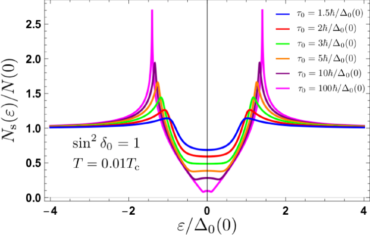
Figure 11: Quasiparticle DOS $N_{\rm s}(\varepsilon)$ normalized by the normal DOS at the Fermi surface $N(0)$ for the different normal relaxation times $\tau_{0}=1.5\hbar/\Delta_{0}(0)$, $2\hbar/\Delta_{0}(0)$, …, 100 $\hbar/\Delta_{0}(0)$ in the unitarity limit as $\sin^{2}\delta_{0}=1$ at $T=0.01T_{\rm c}$.

IV.1 Volovik effect

We first discuss the Doppler shift effect on the thermal conductivity and the thermal Hall angle in $d$-wave superconductors. It is shown that the Doppler shift effect can be neglected at very weak magnetic fields. In this subsection, we fix the parameters as $\sin^{2}\delta_{0}=0$ (the Born-type impurity) and $\tau_{0}=10\hbar/\Delta_{0}(0)$.

Figure 1 plots the longitudinal thermal conductivity $\kappa_{xx}$ normalized by the value at the transition temperature without impurities and external fields $T_{\rm c}$, for different vortex radii $R=7\xi_{0}(0),10\xi_{0}(0),\dots,\infty$ as a function of temperature. The thermal conductivity for $R\to\infty$ are the same as that for ${\bm{v}}_{\rm s}={\bm{0}}$. We observe that the normalized longitudinal thermal conductivity decreases as temperature decreases from $T=T_{\rm c}$, and $T$-linear behavior for $d$-wave superconductors at low temperatures. These behaviors at low temperatures are well-known results Coffey ; Graf .

Figure 2 plots the thermal Hall conductivity $\kappa_{xy}$ normalized by the value at the transition temperature without impurities and external fields $T_{\rm c}$, for the different vortex radii $R=7\xi_{0}(0),10\xi_{0}(0),\dots,\infty$ as a function of temperature. We observe that the normalized thermal Hall conductivity varies more as a function of the vortex radius compared with the longitudinal component. The normalized thermal Hall conductivity has a finite value even near $T=0$, and decreases significantly around $T=0.05T_{\rm c}$ as the vortex radius decreases from $R\to\infty$. We here note that the thermal Hall conductivity (without the normalization) is proportional to the magnetic field in the temperature range where the normalized thermal Hall conductivity does not change as a function of the vortex radius, since the thermal Hall conductivity at $T=T_{\rm c}$ used to normalize is also proportional to the magnetic field as seen in Eq. (39b). It means that the Doppler shift effect is very small in the temperature range where the normalized thermal Hall conductivity does not almost change.

Figure 3 plots the thermal Hall angle $\tan\theta_{\rm H}\equiv\kappa_{xy}/\kappa_{xx}$ normalized by the value at the transition temperature without impurities and external fields $T_{\rm c}$, for the different vortex radii $R=7\xi_{0}(0),10\xi_{0}(0),\dots,\infty$ as a function of temperature. We observe that the normalized thermal Hall angle greatly enhanced in $d$-wave superconductors.

We confirmed that the normalized thermal conductivity and the normalized thermal Hall angle approach that for ${\bm{v}}_{\rm s}={\bm{0}}$ as the vortex radius $R$ increases, and the normalized thermal conductivity and the normalized thermal Hall angle for ${\bm{v}}_{\rm s}={\bm{0}}$ are almost equal to that at $R=1000\xi_{0}(0)$ within $T\geq 0.01T_{\rm c}$.

IV.2 Impurity effect

We finally discuss the impurity effect on the thermal conductivity and the thermal Hall angle normalized by the value at the transition temperature without impurities and external fields $T_{\rm c}$ in $d$-wave superconductors for ${\bm{v}}_{\rm s}={\bm{0}}$, since the experimental results on the longitudinal thermal conductivity in heavy-fermion superconductors and Zn-doped YBCO were explained by taking into account impurity scattering close to the unitarity limit Coffey ; Hirschfeld96 ; Schmitt ; Hirschfeld88 , and $\tan\theta_{\rm H}/H$ and $\kappa_{xy}/H$ in the zero magnetic-field limit $H\to 0$ were estimated experimentally by the initial slope in the $H$ dependence of $\kappa_{xy}$ in Refs. Zhang01, and Kasahara, . The thermal Hall conductivity and the thermal Hall angle at $T=T_{\rm c}$ used to normalize are proportional to the “internal” magnetic field $B$ [see Eq. (39b)], and the internal magnetic field $B$ in extreme type-II superconductors also approaches zero as the external magnetic field $H$ approaches zero. Thus, the normalized thermal Hall conductivity and the normalized thermal Hall angle in extreme type-II superconductors for ${\bm{v}}_{\rm s}={\bm{0}}$ are the same as evaluating $\lim_{H\to 0}\tan\theta_{\rm H}/H$ and $\lim_{H\to 0}\kappa_{xy}/H$. Here we discuss the contribution from the scattering of quasiparticles on vortices Durst . The thermal Hall conductivity due to the vortex scattering at weak magnetic fields is given by $\kappa_{xy}^{\rm vortex}\sim T\sqrt{H}$. Since $\kappa_{xy}^{\rm vortex}/H$ diverges for $H\to 0$ regardless of temperature, and the longitudinal thermal conductivity is given by $\kappa_{xx}\sim T$, $\tan\theta_{\rm H}/H$, and $\kappa_{xy}/H$ for $H\to 0$ are dominated by the Lorentz force and the impurities. Therefore, we can study the impurity effect on thermally excited quasiparticles outside the core in extreme type-II superconductors, estimating $\lim_{H\to 0}\tan\theta_{\rm H}/H$ and $\lim_{H\to 0}\kappa_{xy}/H$ experimentally.

Figures 4, 5, 6, and 7 plot the longitudinal thermal conductivity $\kappa_{xx}$ and $\kappa_{xx}/T$, the thermal Hall conductivity $\kappa_{xy}$, and the thermal Hall angle $\tan\theta_{\rm H}$ normalized by the value at the transition temperature without impurities and external fields $T_{\rm c}$, for the different scattering phase shifts $\sin^{2}\delta_{0}=0,0.2,\dots,1$ at the normal relaxation time $\tau_{0}=10\hbar/\Delta_{0}(0)$ as a function of temperature. We reproduce the longitudinal thermal conductivity $\kappa_{xx}$ proposed by Graf et al. Graf , and show that the behavior of the normalized thermal Hall conductivity is similar to that of the normalized longitudinal thermal conductivity. We also observe that the enhancement of the normalized thermal Hall angle near zero temperature decreases as $\sin^{2}\delta_{0}$ increases from $\sin^{2}\delta_{0}=0$, and does not occur at $\sin^{2}\delta_{0}=1$. Figures 8 and 9 plot the thermal Hall angle normalized by the value at the transition temperature without impurities and external fields $T_{\rm c}$, for the different normal relaxation times $\tau_{0}=1.5\hbar/\Delta_{0}(0),2\hbar/\Delta_{0}(0),\dots,100\hbar/\Delta_{0}(0)$ in the Born and unitarity limit as $\sin^{2}\delta_{0}=0$ and $1$, respectively, as a function of temperature. It is shown that the normalized thermal Hall angle is greatly enhanced in the Born limit as $\sin^{2}\delta_{0}=0$ near zero temperature but is suppressed in the unitarity limit as $\sin^{2}\delta_{0}=1$ near zero temperature even at the large normal relaxation time $\tau_{0}=100\hbar/\Delta_{0}(0)$. We can explain the normal relaxation time and temperature dependence of the normalized thermal Hall angle in the Born and unitarity limit as follows, using the corresponding quasiparticle DOS in Figs. 10 and 11.

We first consider the Born-type impurity as $\sin^{2}\delta_{0}=0$. Then the quasiparticle relaxation time $\tau_{\rm QP}$ can be written from Eq. (35) as $\tau_{\rm QP}=\tau_{0}/\langle{\rm Re}g_{0}^{\rm R}\rangle_{\rm F}$ near zero temperature, since quasiparticles around the gap nodes at $\phi=0$ become dominant. Furthermore, in the $d$-wave pairing case, since the quasiparticle DOS has a finite small value near $\varepsilon=0$, the impurity scattering for quasiparticles near $\varepsilon=0$ is very small. We can also explain that the quasiparticle impurity scattering is very small near zero temperature, since quasiparticles around the gap nodes are restricted to the momentum in a specific orientation. In the Born limit, the normalized thermal Hall angle near zero temperature can be roughly written as

$$\frac{\tan\theta_{H}(T)}{\tan\theta_{H}(T_{\rm c})}\sim\int d\varepsilon\frac{1}{\langle{\rm Re}g_{0}^{\rm R}\rangle_{\rm F}}{\rm sech}^{2}\frac{\varepsilon}{2k_{\rm B}T},$$ (41)

where the $\varepsilon$ integration signifies an integration over $-\infty\leq\varepsilon\leq\infty$, except $\langle{\rm Re}g_{0}^{\rm R}\rangle_{\rm F}=0$. Thus, the normalized thermal Hall angle is more enhanced in the Born limit at the large normal relaxation time near zero temperature, since the quasiparticle DOS near $\varepsilon=0$ becomes small as the normal relaxation time increases, as seen in Fig. 10. On the other hand, when taking the unitarity limit as $\sin^{2}\delta_{0}=1$, the quasiparticle relaxation time $\tau_{\rm QP}$ near zero temperature can be given by $\tau_{\rm QP}=\tau_{0}\langle{\rm Re}g_{0}^{\rm R}\rangle_{\rm F}$, and the restriction on the direction of the quasiparticle momentum is relaxed due to the strong scattering effect. In the unitarity limit, the normalized thermal Hall angle near zero temperature can be also roughly written as

$$\frac{\tan\theta_{H}(T)}{\tan\theta_{H}(T_{\rm c})}\sim\int d\varepsilon\langle{\rm Re}g_{0}^{\rm R}\rangle_{\rm F}{\rm sech}^{2}\frac{\varepsilon}{2k_{\rm B}T}.$$ (42)

Thus, the normalized thermal Hall angle in the the unitarity limit is more suppressed at the large normal-relaxation-time near zero temperature inversely to the Born-type impurity, since the quasiparticle DOS near $\varepsilon=0$ is smaller as $\tau_{0}$ increases, as seen Fig. 11. However, since the thermal conductivity in $d$-wave superconductors with scattering close to the unitarity limit is also almost zero at low temperature, it may be difficult to observe the suppression of the Hall angle experimentally.

In our results, the normalized thermal Hall angle near zero temperature was up to about $100$ times larger than that at the transition temperature. From the figures in Refs. Zhang01, and Kasahara, estimating roughly the ratio of the thermal Hall angle at zero temperature to that at the transition temperature, that in Ref. Zhang01, is about 100, and that in Ref. Kasahara, is about 15. Here we note that these thermal-Hall-angle ratios were estimated in the limit of zero magnetic field. The thermal-Hall-angle ratio in Ref. Zhang01, is approximately consistent with our result for the large normal relaxation time in the Born limit, and that in Ref. Kasahara, is almost the same as the result for $\tau_{0}=100\hbar/\Delta_{0}(0)$ and $\sin^{2}\delta_{0}=0.8$, or $\tau_{0}=10\hbar/\Delta_{0}(0)$ and $\sin^{2}\delta_{0}=0.6$, or …, or $\tau_{0}=2\hbar/\Delta_{0}(0)$ and $\sin^{2}\delta_{0}=0$. Thus, we find from calculations of the thermal Hall angle that YBCO in Ref. Zhang01, is very clean, and materials in Ref. Kasahara, is relatively dirty within this our present theory.

V Concluding remarks

We derived the thermal conductivity in extreme type-II superconductors with an isolated pinned vortex based on the augmented quasiclassical equations of superconductivity with the Lorentz force. Using it, we calculated the thermal conductivity and the thermal Hall angle in $d$-wave superconductors, and addressed the enhancement of $\lim_{H\to 0}\tan\theta_{\rm H}/H$ at low temperatures in YBCO and CeCoIn₅ measured by Zhang et al. Zhang01 and by Kasahara et al. Kasahara . They estimated $\lim_{H\to 0}\tan\theta_{\rm H}/H$ using the initial slope in the $H$ dependence of $\kappa_{xy}$ measured experimentally. We also should point out that since the superfluid velocity ${\bm{v}}_{\rm s}$ is proportional to $1/\rho$, the Doppler shift effect has the potential to contribute to the spatial average of the thermal conductivity and the thermal Hall angle. Thus, we calculated the magnetic-field dependence of $\tan\theta_{\rm H}$ and $\kappa_{xy}$ due to the Doppler shift effect, and confirmed that the Doppler shift effect can be neglected in the limit $H\to 0$.

The thermal Hall conductivity due to the vortex scattering at weak magnetic fields proposed by Durst et al. in Ref. Durst, is given by $\kappa_{xy}^{\rm vortex}=C_{0}T\sqrt{H}$, where $C_{0}$ is a constant introduced in Ref. Durst, , and it has been used successfully to explain the experimental results on the magnetic field dependence of the thermal conductivity in YBa₂Cu₃O_6.99 in the weak magnetic-field region. However, they did not address the enhancement of $\lim_{H\to 0}\tan\theta_{\rm H}/H$ at low temperatures even in Refs. Ganeshan, and Kulkarni, , which are their more recent papers, and we cannot explain this enhancement using their theories. Unlike our theory, since their theory takes into account only the contribution of quasiparticles around the gap nodes, it is impossible to investigate the wide temperature dependence from the transition temperature to zero temperature. Moreover, $\kappa_{xy}^{\rm vortex}$ is proportional to $\sqrt{H}$, and $\kappa_{xy}^{\rm vortex}/H$ diverges for $H\to 0$, i.e., the quasiparticle relaxation time due to the vortex scattering diverges for $H\to 0$ regardless of temperature, since the longitudinal thermal conductivity becomes $\kappa_{xx}\sim T$ for $H\to 0$. On the other hand, the thermal Hall conductivity due to the Lorentz force $\kappa_{xy}^{\rm Lorentz}$ is proportional to $H$ [see Eq. (34)], and $\kappa_{xy}^{\rm Lorentz}/H$ has a finite value for $H\to 0$. Therefore, $\lim_{H\to 0}\tan\theta_{\rm H}/H$ and $\lim_{H\to 0}\kappa_{xy}/H$ are dominated by the Lorentz force and the impurities. We observed that the thermal Hall angle is greatly enhanced in $d$-wave superconductors without impurities of the resonant scattering at low temperatures and very weak magnetic field. This great enhancement of the thermal Hall angle has been observed experimentally in YBCO Zhang01 and CeCoIn₅ Kasahara , and may also be observed experimentally in other nodal superconductors with large magnetic-penetration-depth.

On the other hand, our absolute values of the thermal conductivity are different from the experimental values. To discuss the experimental values more quantitatively, we may need to consider inelastic scattering as considered in the calculation of the longitudinal component, such as scattering by the antiferromagnetic spin fluctuations within the RPA Hirschfeld96 or the fluctuation exchange approximation Hara in YBCO. The relaxation times for inelastic scattering in the superconducting phase of UPt₃ and CeCoIn₅ are also given in Refs. Fledderjohann, and Graf96, , and Truncik, . Here we emphasize that the great enhancement of the electrical and longitudinal thermal conductivity in the superconducting state of YBCO is dominated by the contribution from inelastic scattering Hirschfeld96 , but thermal Hall angle is greatly enhanced in nodal superconductors even without inelastic scattering.

We also discuss the contribution from quasiparticles in the vortex core. For clean superconductors in the vortex lattice state under larger magnetic field, we should consider the contribution of quasiparticles in the vortex core. The thermal Hall angle in the vortex lattice state may decrease due to the increase in quasiparticle scattering in the vortex core as the external magnetic field increases Kasahara , but we also need to calculate it microscopically and quantitatively to clarify the suppression of the thermal Hall angle due to external magnetic field. We may confirm this by solving the augmented quasiclassical equations directly in the vortex lattice system Adachi ; Ichioka99 (see Ref. Ueki18, for the pair-potential-gradient force and the pressure difference arising from the slope in the DOS). This method can include not only the contribution of quasiparticles outside the core but also that of the Andreev-reflected quasiparticles Dahm ; Nagai in the thermal conductivity. We may also calculate the thermal Hall conductivity in high magnetic fields more easily, using the Brandt–Pesch–Tewordt approximation for the augmented quasiclassical equations Houghton . Moreover, we may also need to confirm the contributions from skew scattering due to a vortex Durst ; Kulkarni and the Berry phase acquired by a quasiparticle on traversing around a vortex Vafek01 ; Cvetkovic ; Murray ; Vafek15 ; Ganeshan in the calculations under larger magnetic field.

Our approach for the study of thermal Hall conductivity in type-II superconductors can be applied to the microscopic study of quasiparticle transport in a variety of superconductors under magnetic field.

References

• (1) J. L. Cohn, M. S. Osofsky, J. L. Peng, Z. Y. Li, and R. L. Greene, Phys. Rev. B 46, 12053 (1992).
• (2) K. Krishana, J. M. Harris, and N. P. Ong, Phys. Rev. Lett. 75, 3529 (1995).
• (3) B. Zeini, A. Freimuth, B. BΓΌchner, R. Gross, A. P. Kampf, M. KlΓ€ser, and G. MΓΌller-Vogt, Phys. Rev. Lett. 82, 2175 (1999).
• (4) K. Krishana, N. P. Ong, Y. Zhang, Z. A. Xu, R. Gagnon and L. Taillefer, Phys. Rev. Lett. 82, 5108 (1999).
• (5) Y. Zhang, N. P. Ong, Z. A. Xu, K. Krishana, R. Gagnon, and L. Taillefer, Phys. Rev. Lett. 84, 2219 (2000).
• (6) R. OcaΓ±a, A. Taldenkov, P. Esquinazi, and Y. Kopelevich, J. Low. Temp. Phys. 123, 181 (2001).
• (7) Y. Zhang, N. P. Ong, P. W. Anderson, D. A. Bonn, R. Liang, and W. N. Hardy, Phys. Rev. Lett. 86, 890 (2001).
• (8) B. Zeini, A. Freimuth, B. BΓΌchner, M. Galffy, R. Gross, A. P. Kampf, M. KlΓ€ser, G. MΓΌller-Vogt, and L. Winkler, Eur. Phys. J. B 20, 189 (2001).
• (9) Y. Kasahara, Y. Nakajima, K. Izawa, Y. Matsuda, K. Behnia, H. Shishido, R. Settai, and Y. Onuki, Phys. Rev. B 72, 214515 (2005).
• (10) S. H. Simon and P. A. Lee, Phys. Rev. Lett. 78, 1548 (1997).
• (11) P. J. Hirschfeld, and W. O. Putikka, Phys. Rev. Lett. 77, 3909 (1996).
• (12) J. Bardeen, G. Rickayzen, and L. Tewordt, Phys. Rev. 113, 982 (1959).
• (13) M. J. Graf, S.-K. Yip, J. A. Sauls, and D. Rainer, Phys. Rev. B 53, 15147 (1996).
• (14) H. Adachi, P. MiranoviΔ‡, M. Ichioka, and K. Machida, J. Phys. Soc. Jpn. 76, 064708 (2007).
• (15) S. Schmitt-Rink, K. Miyake, and C. M. Varma, Phys. Rev. Lett. 57, 2575 (1986).
• (16) P. J. Hirschfeld, P. WΓΆlfle, and D. Einzel, Phys. Rev. B 37, 83 (1988).
• (17) C. KΓΌbert and P. J. Hirschfeld, Phys. Rev. Lett. 80, 4963 (1998).
• (18) M. Franz, Phys. Rev. Lett. 82, 1760 (1999).
• (19) I. Vekhter and A. Houghton, Phys. Rev. Lett. 83, 4626 (1999).
• (20) A. B. Vorontsov and I. Vekhter, Phys. Rev. B 75, 224502 (2007).
• (21) H. Hara, and H. Kontani, J. Phys. Soc. Jpn. 76, 073705 (2007).
• (22) T. Kobayashi, T. Matsushita, T. Mizushima, A. Tsuruta, and S. Fujimoto, Phys. Rev. Lett. 121, 207002 (2018).
• (23) N. Read and D. Green, Phys. Rev. B 61, 10267 (2000).
• (24) K. Nomura, S. Ryu, A. Furusaki, and N. Nagaosa, Phys. Rev. Lett. 108, 026802 (2012).
• (25) H. Sumiyoshi and S. Fujimoto, J. Phys. Soc. Jpn. 82, 023602 (2013).
• (26) Y. Imai, K. Wakabayashi, and M. Sigrist, Phys. Rev. B 93, 024510 (2016).
• (27) N. Yoshioka, Y. Imai, and M. Sigrist, J. Phys. Soc. Jpn. 87, 124602 (2018).
• (28) S. Yip, Supercond. Sci. Technol. 29, 085006 (2016).
• (29) F. YΔ±lmaz and S. Yip, arXiv:1911.00711.
• (30) V. Ngampruetikorn and J. A. Sauls, arXiv:1911.06299.
• (31) V. Ngampruetikorn and J. A. Sauls, Phys. Rev. Lett. 124, 157002 (2020).
• (32) A. C. Durst, A. Vishwanath, and P. A. Lee, Phys. Rev. Lett. 90, 187002 (2003).
• (33) O. Vafek, A. Melikyan, and Z. TeΕ‘anoviΔ‡, Phys. Rev. B 64, 224508 (2001).
• (34) V. Cvetkovic and O. Vafek, Nat. Commun. 6, 6518 (2015).
• (35) J. M. Murray and O. Vafek, Phys. Rev. B 92, 134520 (2015).
• (36) O. Vafek, Phys. Rev. B 92, 174508 (2015).
• (37) A. Shahzamanian, H. Yavary, and A. Yousefvand, Phys. Stat. Sol. (c) 3, 3148 (2006).
• (38) G. Eilenberger, Z. Phys. 214, 195 (1968).
• (39) M. Eschrig, J. A. Sauls, and D. Rainer, Phys. Rev. B 60, 10447 (1999).
• (40) Y. Kato and C.-K. Chung, J. Phys. Soc. Jpn. 85, 033703 (2016).
• (41) T. Kita, Phys. Rev. B 64, 054503 (2001).
• (42) L. P. Gor’kov, Zh. Eksp. Teor. Fiz. 36, 1918 (1959) [Sov. Phys. JETP 9, 1364 (1959)].
• (43) L. P. Gor’kov, Zh. Eksp. Teor. Fiz. 37, 1407 (1959) [Sov. Phys. JETP 10, 998 (1960)].
• (44) E. Arahata and Y. Kato, J. Low. Temp. Phys. 175, 364 (2014).
• (45) G. E. Volovik, JETP Lett. 58, 469 (1993).
• (46) N. B. Kopnin and G. E. Volovik, JETP Lett. 64, 690 (1996).
• (47) T. Dahm, S. Graser, C. Iniotakis, and N. Schopohl, Phys. Rev. B 66, 144515 (2002).
• (48) Y. Nagai and N. Hayashi, Phys. Rev. Lett. 101, 097001 (2008).
• (49) L. Coffey, T. M. Rice, and K. Ueda, J. Phys. C 18, L813 (1985).
• (50) Y. Kato, J. Phys. Soc. Jpn. 69, 3378 (2000).
• (51) M. Ohuchi, H. Ueki, and T. Kita, J. Phys. Soc. Jpn. 86, 073702 (2017).
• (52) Y. Masaki and Y. Kato, J. Phys.: Conf. Ser. 969, 012054 (2018).
• (53) Y. Masaki, Phys. Rev. B 99, 054512 (2019).
• (54) H. Ueki, M. Ohuchi, T. Kita, J. Phys. Soc. Jpn. 87, 044704 (2018).
• (55) V. L. Ginzburg, Sov. Phys. Usp. 34, 101 (1991).
• (56) K. Izawa, K. Behnia, Y. Matsuda, H. Shishido, R. Settai, Y. Onuki, and J. Flouquet, Phys. Rev. Lett. 99, 147005 (2007).
• (57) H. Ueki, W. Kohno, and T. Kita, J. Phys. Soc. Jpn. 85, 064702 (2016).
• (58) T. Kita, Phys. Rev. B 79, 024521 (2009).
• (59) S. Ganeshan, M. Kulkarni, and A. C. Durst, Phys. Rev. B 84, 064503 (2011).
• (60) M. Kulkarni, S. Ganeshan, and A. C. Durst, Phys. Rev. B 84, 064502 (2011).
• (61) A. Fledderjohann and P. J. Hirschfeld, Solid State Commun. 94, 163 (1995).
• (62) M. J. Graf, S.-K. Yip, and J. A. Sauls, J. Low. Temp. Phys. 102, 367 (1996).
• (63) C. J. S. Truncik, W. A. Huttema, P. J. Turner, S. Γ–zcan, N. C. Murphy, P. R. Carrire, E. Thewalt, K. J. Morse, A. J. Koenig, J. L. Sarrao, and D. M. Broun, Nat. Commun. 4, 2477 (2013).
• (64) M. Ichioka, A. Hasegawa, and K. Machida, Phys. Rev. B 59, 8902 (1999).
• (65) A. Houghton and I. Vekhter, Phys. Rev. B 57, 10831 (1998).