Large-scale interactive object segmentation with human annotators

Abstract

Manually annotating object segmentation masks is very time consuming. Interactive object segmentation methods offer a more efficient alternative where a human annotator and a machine segmentation model collaborate. In this paper we make several contributions to interactive segmentation: (1) we systematically explore in simulation the design space of deep interactive segmentation models and report new insights and caveats; (2) we execute a large-scale annotation campaign with real human annotators, producing masks for 2.5M instances on the OpenImages dataset. We plan to release this data publicly, forming the largest existing dataset for instance segmentation. Moreover, by re-annotating part of the COCO dataset, we show that we can produce instance masks $3\times$ faster than traditional polygon drawing tools while also providing better quality. (3) We present a technique for automatically estimating the quality of the produced masks which exploits indirect signals from the annotation process.

1 Introduction

Propelled by the increased computing power, the last years have seen a dramatic growth in the size of models for computer vision tasks. These larger models are evermore demanding of larger training sets to reach performance saturation [32]. This demand for data often becomes a bottleneck for practitioners. While computers become cheaper, faster, and able to handle larger models, the cost of humans manually annotating data remains very high. Hence, we need new strategies to scale-up human annotations.

Amongst the traditional image understanding tasks, instance segmentation is considered one of the most expensive to annotate [8, 19, 6, 37]. For each object instance in each class of interest, it requires annotating a mask indicating which pixels belong to the instance.

In this work we explore an interactive segmentation approach to annotate instance masks, where the human annotator focuses on correcting the output of a segmentation model, rather than spending time blindly creating full annotations that might be redundant or already captured by the model. Across multiple rounds the annotator provides corrections to the current segmentation, and then the model incorporates them to refine the segmentation.

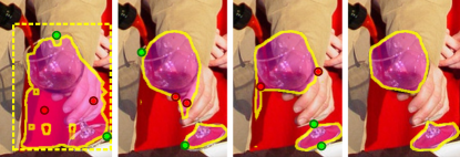
Figure 1: Example of corrective clicks and their effect on the segmentation mask. Starting from a bounding box, the annotator provides up to $4$ corrective clicks in each round. See section 2.

Albeit the idea of interactive segmentation was established already a decade ago [4, 30], we make two key contributions: (1) through extensive simulations we systematically explore the design space of deep interactive segmentations models and report new insights and caveats (Sec. 3). (2) while most previous works report only simulation experiments [36, 35, 17, 20, 10, 22], we execute a large-scale annotation campaign with real human annotators (2.5M instances, Sec. 4), we analyse the annotators behavior (Sec. 5.2) and the resulting annotations (Sec. 5.3).

Our results show that we can make instance segmentation $3\times$ faster than traditional polygon drawing tools [19] while also providing better quality (Sec. 5.3). Additionally our method can produce masks across different time budgets, and we present a new technique for automatically estimating the quality of the produced masks which exploits indirect signals from the annotation process (Sec. 5.4).

To the best of our knowledge this is the first work exploring interactive annotations at scale. We apply our approach to collect $2.5\text{M}$ new masks over $300$ categories of the OpenImages dataset [14]. We plan to release the data mid-2019, making it the largest public dataset for instance segmentation (in the number of instances).

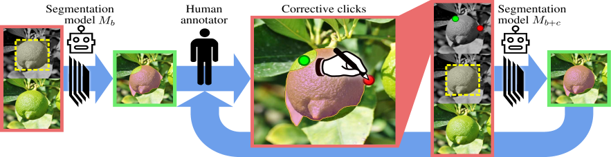
Figure 2: High level overview of our interactive annotation system ($M_{r}$ not shown). See description in section 2.

1.1 Related work

Dataset annotations

A flurry of techniques have been explored to annotate the location of objects in images: bounding box annotations [8], clicks on the object extremes [26, 22], clicks on the object centre [3, 27], bounding box followed by edits to a generated segment [4, 30], scribbles [3, 18], hierarchical super-pixel annotations [21], polygon annotations [8, 9, 19], interactive polygons [1], eye gaze [25], and touch interfaces [28], just to name a few.
Despite many explored ideas, the current most popular datasets for object instances localization were all obtained using purely manual annotations of boxes or (layered) polygons [8, 31, 9, 19, 6, 24, 11, 37].
This work aims at changing the status quo by showing the interest of interactive instance segmentation as main annotation strategy for large scale instance segmentation.

Weakly supervised segmentation

Weakly supervised segmentation methods reconstruct approximate segmentation masks starting from weaker supervision input. For semantic/instance segmentation the following sources of supervision have been explored: image level label only [38], point clicks [3, 36], boxes only [7, 12, 35], scribbles only [18, 3], boxes plus clicks [4, 30, 35, 26, 22].
Most interactive segmentation techniques build upon weakly supervised methods. Our work starts from segments generated from boxes, and then moves into an interactive mode by adding corrective clicks as additional supervision.

Interactive segmentation

The idea of interactive image segmentation is decades old [4, 30]. It has been revisited in the recent years under the deep learning umbrella [36, 20, 10, 34, 22, 16, 15, 1], focusing on how to best use clicks and scribbles corrections. Most of these work share structural similarities but diverge in their finer design choices (e.g. annotation type, input encoding, etc.). Section 3 revisits some of these choices in an unified experimental setup and draws new conclusions.

Despite the theme of human-machine interaction, most previous work in this area report purely simulation experiments [35, 17, 20, 22] or only small scale human experiments ($\leq 50$ instances [15, 16, 1]). We instead collect $2.5\text{M}$ masks over 300 categories using a team of 100 annotators, share the learned lessons, and analyse the resulting annotations when considering interactive segmentation at scale.

2 Overall system design

We propose a design that involves three types of models $M_{b}$, $M_{b+c}$, $M_{r}$. Starting from existing bounding boxes for each instance, we generate initial masks via an "image$+$box$\rightarrow$mask" model $M_{b}$. We then show these masks to human annotators, which indicate corrections. These corrections are used as supervision to generate new improved masks, via an "image$+$box$+$corrections$\rightarrow$mask" model $M_{b+c}$. The annotators iteratively correct the outputs of $M_{b+c}$ over multiple rounds (figure 2). The final instance segmentation model is thus trained using as privileged information the initial bounding boxes and the corrections provided throughout the process.

Models $M_{b}$ and $M_{b+c}$ are implemented using convnets, while $M_{r}$ is a decision forest. Compared to previous work on interactive segmentation such as [20, 16, 1] we use a different design for $M_{b}$ / $M_{b+c}$, and introduce the use of a ranking model $M_{r}$. This ranking model uses the time sequence of annotator corrections on an instance to predict the expected quality of the generated mask. This ranking can be used to prioritise further corrections on low quality instances, or as weighting signal when training an instance segmentation model. In section 3 we study the design of $M_{b}$ and $M_{b+c}$; and in section 4 we describe a concrete instantiation of our approach. The ranking model $M_{r}$ is described in section 4.2.

Since annotators spend their time solely on corrections, the data collected is directly focused on areas not yet correctly captured by the $M_{b}$/$M_{b+c}$ models. Easy instances will need zero edits from the get go, while hard instances might need multiple revisits.

3 Simulations

The generic system described in section 2 has many free design parameters, and previous related works have reported contradicting results. Section 3.1 describes an implementation blueprint of our system, and section 3.2 reports simulation results exploring its design space.

3.1 Experiments blueprint

Evaluation set

For these experiments we use COCO [19], which is considered the gold standard amongst existing instance segmentation datasets. COCO was annotated by manually drawing polygons on object instances. Albeit some previous interactive segmentation works report COCO results [36, 17, 16, 10], they only consider $\leq 20$ instances per class; here we consider a larger set of $\sim\negmedspace 88k$ instances.
COCO objects have a median size of $53\times 62$ pixels. Small objects tend to have blob-like shapes, while larger objects show more detail. We thus focus training and evaluation only on instances larger than $80\times 80\ \text{pixels}$. We evaluate results over the large instances in the COCO 2014 validation set (41k images), which we denote as $\text{COCO}_{\text{L}}^{\text{test}}$.

Training set

The training set of $M_{b}$ and $M_{b+c}$ will have a direct impact on the effectiveness of the interactive annotation system. We train our models over a subset of the ADE20k training set [37]. We picked the 255 largest classes representing objects (window, leg, lamp, etc.) and left out stuff classes (wall, sky, sidewalk, etc.). In total these have $\sim\negmedspace 400k$ instances. After filtering by size, we are left with $\sim\negmedspace 134k$ instances with ground-truth segmentations. We name this training set $\text{ADE}_{\text{L}}^{\text{train}}$. Unless otherwise specified, we train our models on it in a class-agnostic way: considering all instances as belonging to a single generic object class. We split $\text{ADE}_{\text{L}}^{\text{train}}$ in two halves to train $M_{b}$ over $\text{ADE}_{\text{L\ $\nicefrac{{1}}{{2}}$}}^{\text{train}}$ , and $M_{b+c}$ over $\text{ADE}_{\text{L\ $\nicefrac{{2}}{{2}}$}}^{\text{train}}$.
Unless otherwise specified all instances are cropped and scaled to fit inside a $193\times 193\ \text{pixels}$ box (keeping their aspect ratio) centred in a $385\times 385\ \text{pixels}$ image (capturing some of the instance context, or padding borders with black pixels if outside of source image).
The ranking model $M_{r}$ is trained over a small set of real corrective click annotations and ground-truth masks (§4.2).

We treat both training and testing on a per-instance basis, and ignore class labels (i.e. we average across instances). We use the traditional mean intersection-over-union (mIoU) as our main evaluation metric.

Annotator simulation

Training $M_{b}$ requires ground-instance segmentations, and training $M_{b+c}$ additionally requires annotator corrections. These training corrections can be collected by running annotation campaigns over data with already available ground-truth segmentations, or can be generated by simulating the expected annotator behavior. In the latter case, the details of the simulations matter. The assumptions underlying the simulated corrections should match the expected behavior of annotators. Moreover, depending on how much error we expect from the annotators (noise model), the simulation results will have higher or lower IoU. This is a confounding factor when comparing results amongst related works. Also, if we train with a certain annotator noise model, and test with the same model, results might be over-optimistic (compared to using actual human annotators).

Our simulations include noise both on the boxes and the clicks. We generate object bounding boxes by perturbing the corners of a perfect bounding box fit to the ground-truth segmentation with $\mathcal{N}\left(0,\,60\ \text{pixels}\right)$ noise. We keep bounding boxes with $\text{IoU}\geq 0.7$ with the tight ground-truth box. We use such loose boxes because: a) depending on their source, not all boxes are expected to be very tight; b) we expect to encounter cases where there is a drift between the box annotation policies and the segmentation policies (section 4.3). Furthermore, we perturb corrective clicks with $\mathcal{N}\left(0,\,3\ \text{pixels}\right)$. The initial click location is also randomly sampled following a probability distributions specific to the click type (section 3.2.2). Also, some error regions might be ignored if deemed too small (section 3.2.3).
Unless otherwise stated, each simulation runs for 3 rounds of interaction, with the simulated annotator providing up to 3 clicks per round (which we denote as $3\times 3$). Section 3.2.5 studies how to distribute corrective clicks across rounds.

Models

Both $M_{b}$ and $M_{b+c}$ use the same architecture. We train Deeplabv2 ResNet101 [5] for per-pixel binary classification (instance foreground/background). See supplementary material for training parameters. The Deeplab model is augmented to accept N-channels input instead of only an RGB image. $M_{b}$ uses 4 channels, RGB plus a binary bounding box image (inside/outside). $M_{b+c}$ uses 5 or more channels, RGB + box + corrections. Previous works have used different strategies to encode the corrections, which we explore in section 3.2.4. Our ranking model $M_{r}$ is a decision forest described in section 4.2.
By default, we train $M_{b+c}$ to handle $3\times 3$ rounds. We do this by training a single model to use as inputs the cropped RGB image, the binary bounding box, and a variable number of clicks between 1 and 9 (random, uniform discrete distribution). Clicks are encoded as small binary disks (section 3.2.4). We first train the $M_{b}$ model over $\text{ADE}_{\text{L\ $\nicefrac{{1}}{{2}}$}}^{\text{train}}$. Then we train $M_{b+c}$ using simulated corrective clicks on $\text{ADE}_{\text{L\ $\nicefrac{{2}}{{2}}$}}^{\text{train}}$ over masks generated by $M_{b}$.

3.2 Simulation results

Most experiments in this section require re-training both $M_{b}$ and $M_{b+c}$. Together they represent over 9 GPU-months of training time.

3.2.1 $M_{b}$ baselines

When training $M_{b}$ over $\text{ADE}_{\text{L\ $\nicefrac{{1}}{{2}}$}}^{\text{train}}$ we obtain a mean IoU of $65\%$ on $\text{COCO}_{\text{L}}^{\text{test}}$. This is the starting point for our annotations. For comparison using the raw (noisy) bounding boxes as masks, we obtain $50\%\ \text{mIoU}$. A well-tuned Grabcut implementation reaches $59\%\ \text{mIoU}$ [26]. Overall our class-agnostic transfer from ADE20k to COCO via $M_{b}$ seems to perform well in comparison.

3.2.2 Boundary click or region click?

When considering which corrective clicks should be done over a mask, the existing literature is split between clicks at the object border [26, 22, 15, 1] or clicks inside the error regions [36, 17, 16].

For boundary clicks we train $M_{b+c}$ with all clicks pasted into a single channel, whereas region clicks are encoded in two separate channels depending if the click was done inside or outside the current mask.

At test time, we iteratively simulate the clicks by first adding 3 corrective clicks over the mask created by $M_{b}$, then applying $M_{b+c}$, then adding 3 additional corrective clicks, then re-applying $M_{b+c}$, etc. The corrective clicks are applied simulating either clicks on the boundary of the error regions or in their centre. The likelihood of a click in a error region is proportional to its area. If multiple clicks fall in the same error region, they are spread out to roughly partition it in equal areas (or the boundary in equal lengths).

Result

Both type of clicks bring clear improvements in every round. After three rounds, region clicks reach $80\%\ \text{mIoU}$ while boundary clicks reach only $77\%\ \text{mIoU}$. This trend is consistent across different type of input encoding and number of clicks/rounds. We thus move forward with corrective clicks in the centre of error regions as our main correction strategy.

This result can be explained via: 1) centre region clicks are more robust: after a small perturbation the click is still roughly at the region centre, while noisy boundary clicks are often off, 2) region clicks provide more explicit information about what needs to be added or removed.

3.2.3 Annotation noise

We report the effect of two aspects of the annotator behavior model: (1) how precise is the click of the annotator (click noise)?, (2) which error regions will be considered too small to be clicked on (minimum region size)? If the goal is to get masks annotated as fast as possible, small error regions should be ignored by the annotator since they will have minor impact on mask quality.

Result

We consider the mIoU reached at the end of $3\times 3$ simulations. Compared to zero click noise, adding an isotropic Gaussian click noise with standard deviation $3$ or $6$ pixels causes a $3\%$ and $7\%$ drop in mIoU, respectively. Similarly, if the annotator ignores regions smaller than $x^{2}$ pixels, we observe a drop of $3\%$ or $8\%$ mIoU at $x=20$ or $x=30$, respectively (using click noise 3 pixels). Compounded, these two effects can easily explain away $\sim\negmedspace 5\%$ differences between two reported systems (if the annotation noise model is not specified).

Understanding the sensitivity of the model to annotator noise helps decide how much effort should be put into training the annotators to be precise versus fast.

3.2.4 Clicks encoding

Multiple choices are available for encoding corrective clicks as input to $M_{b+c}$. Previous works considered using a distance transform from the clicks [36, 35, 17, 10, 34, 16], a Gaussian centred on each click [15, 22, 20], or a simple binary disk [3] (see supplementary material for examples). Compared to a binary disk, the distance transform makes it easier for the convnet to reason about relative distances to the clicks. The Gaussian might make it easier for the convnet to localise the exact click centre and to handle cases where two nearby clicks overlap.

Result

The results from figure 3 indicate that using a Gaussian or distance transform, surprisingly, underperforms compared to using a simple binary disk to encode input clicks. The disk diameter seems make little difference. In our setup, simplest is best.

We also tried to add the mask generated from the previous round as an additional input channel, however this did not improve results.

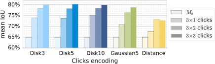
Figure 3: Effect of clicks encoding on the resulting masks. $M_{b}$ indicates the masks obtained with zero clicks (bounding box only). Simple binary disks behave better than the alternatives.

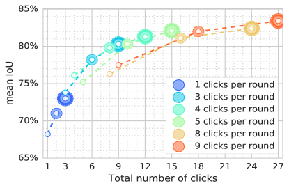
Figure 4: Effect of varying the number of clicks per round. Each curve show three simulated rounds (number of rings = rounds done). If ~9 clicks are to be collected, it is better to do $3\times 3$, $4\times 2$, or $5\times 2$; than to do $1\times 8$ or $1\times 9$. This highlights the benefit of doing clicks that respond to the model error.

3.2.5 Number of clicks and rounds

Region clicks provide direct supervision for the clicked pixels with a foreground or background label. The more clicks the better the resulting masks (with diminishing returns). However it is unclear how to distribute those clicks across rounds. As masks are updated inbetween rounds, it might be good to gather as many clicks as possible per round. However if too many are done before updating the mask presented to the annotator, we under-use the extrapolation power of $M_{b+c}$. One click typically affects the whole region around it and can have global corrective effect on the generated mask (figure 1).

We explore here this trade-off by evaluating three annotation rounds with different number of clicks per round. They all start from the masks generated by the $M_{b}$ model ($65\%\ \text{mIoU}$).

Result

Figure 4 shows a clear gain in mIoU when increasing the total number of corrective clicks, reaching diminishing returns after ~15 clicks. At that point the limits of the $M_{b+c}$ model start to cap the progress of each click. The figure also shows that if one is, for example, aiming for ~9 clicks total, it is better to do $3\times 3$, $4\times 2$, or $5\times 2$ clicks; than to do 8 or 9 clicks all in one round. This highlights the benefits of the interaction between the human annotator and the machine generating the masks; rather than having the annotator blindly clicking on all errors of the initial mask.

3.2.6 Class-agnostic or class-specific?

Up to now $M_{b}$ and $M_{b+c}$ have been trained in a class-agnostic manner. When the target class to annotate is known one might that suspect that using class-specific models might result in higher quality masks.

We experimented training car- and giraffe-specific models and evaluate them over car/giraffes or over all categories. We also trained models from $\text{ADE}_{\text{L}}^{\text{train}}$ (out-of-domain) as well as $\text{COCO}_{\text{L}}^{\text{train}}$ (in-domain).

Result

As expected class-specific $M_{b}$ models generate better initial results. Similarly in-domain models perform slightly better than out-of-domain models. However, when adding annotations the gap between models closes rapidly. After three rounds all variants are within $2$ percent points mIoU. Even training ADE or COCO models without car or giraffe seem to have negligible effect after three rounds. From these results we conclude that there is no need to have class-specific models. Instead a model trained with a large number of instances covering diverse categories performs essentially just as well.

4 Large-scale annotation campaign

Beyond the simulations of section 3, to study the benefits of corrective clicks we also executed a large-scale annotation campaign over the recently released OpenImages V4 dataset [14]. This dataset provides bounding box annotations for 600 object categories. We selected 300 categories for which we make instance masks, based on 1) whether the class exhibits one coherent appearance over which a policy could be defined (e.g. "hicking equiment" is rather ill-defined), 2) whether a clear annotation policy can be defined (e.g. which pixels belong to a nose?, see section 4.3), and 3) whether we expect current segmentation models to be able to capture the shape adequately (e.g. jellyfish contains thin structures that are hard for state-of-the-art models). In total, we annotate 2.5M instances over the 300 OpenImages categories considered. 65 of these overlap with the existing 80 COCO categories. We also re-annotate COCO images for these 65 classes, which allow us to compare with COCO’s manual polygon drawing.

In addition to the annotations generated via corrective clicks, we also make a smaller set of extremely accurate masks fully manually with a free-painting tool (~100 instances per class, for a total of 60k masks). We use these as reference for quality evaluation.

Both corrective clicks and the free-painting annotations are made by a pool of 100 human annotators. These are dedicated full-time annotators, that have a bias towards quality rather than speed.

Section 4.1 describes the exact $M_{b}$ and $M_{b+c}$ models setup for collecting corrective clicks. Section 4.2 describes the ranking model $M_{r}$. Section 4.3 discusses the annotation policies used, and section 4.4 describes the free-painting annotations. We analyse the collected data in section 5.

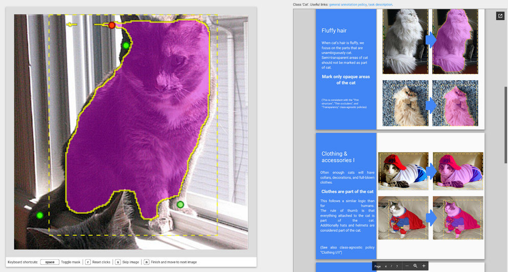
Figure 5: The annotation web interface. Left side shows the object to annotate, the original bounding box (yellow), the current mask (magenta), and the corrective clicks (green and red dots). The right side shows the class-specific policy for the class being annotated.

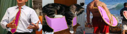
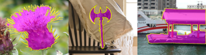
Figure 6: Example of corrective click masks results (top), and free-painting manual annotations (bottom, used as ground-truth reference for evaluations). See supp. material for more examples.

4.1 Corrective clicks setup

For each considered class, we annotate instances from the OpenImages V4 training set with size $\geq\negmedspace 80\negmedspace\times\negmedspace 40$ (or $\geq\negmedspace 40\negmedspace\times\negmedspace 80$) pixels. Based on the simulation results from section 3 we opt to do three rounds of annotations with up to $4$ clicks in each round (i.e. $4\times 3$ setup). Each round is separated by multiple days. We use section’s 3.1 blueprint with region clicks, minimal click region of $10^{2}\ \text{pixels}$, and input clicks encoded in two channels (foreground/background clicks) using binary disks of radius $5\ \text{pixels}$.
To improve the model quality we: (1) increased the resolution of the crops fed into $M_{b}$ and $M_{b+c}$ to $513\negmedspace\times\negmedspace 513$ pixels (object inside $385\negmedspace\times\negmedspace 385$ pixels box); (2) adjusted the clicks noise to mimic the observed annotators behaviour (i.e. near-uniform clicks inside the error regions); (3) added a boundary refinement stage based on [2].

Qualification test

Before starting the main corrective clicks task, each annotator must first pass an automated qualification test to verify the annotator understands the task, how to use the web interface (figure 5), and that he/she is able to perform the task in adequate time. In our experience, using only detailed documentation without an automated qualification test leads to a slow ramp-up towards producing quality annotations.

4.2 Ranking model $M_{r}$

As discussed in section 2, we would like to automatically rank the generated masks from highest quality to lowest quality via a model $M_{r}$. We train our $M_{r}$ model to regress to the IoU of the ground-truth masks. We use a random decision forest with five input features: f1) the number of clicks in the last round; f2) the round number; f3) the $\Delta\text{IoU}$ between the mask from previous round and the one from the current round; f4) the maximum distance between any of the clicks made in the current round and the mask from previous round; and f5) the average distance between the clicks and said mask. The regressor is trained using collected annotations over 1% of $\text{COCO}_{\text{L}}$ instances. We observe that $M_{r}$ training is robust to the volume of training data and the hyper-parameters of the decision forest. Once the ranker $M_{r}$ is trained, we apply it over the full set of COCO and OpenImages corrective click annotations. Examples of ranked masks can be seen in the supp. material.

Out of the five features used, $\Delta\text{IoU}$ and average click distance provide the strongest predictive power. $\Delta\text{IoU}$ encodes how much change happened in the last round. Small changes indicate the mask is already close to its best quality. The average click distance to the mask is a loose indication of the size of the regions being corrected, since annotator are instructed to click near the centre of the error regions. The smaller the error region, the higher the mask quality.

Note that our masks ranker relies solely on indirect signals from the annotation process itself. Since $M_{r}$ does not use class labels (to avoid capturing class biases) nor image features, it generalises well across categories and datasets.

4.3 Annotation policies

An important consideration when dealing with human annotators is that the task must be well specified, otherwise miscommunication could lead to inconsistent outcomes. Compared to drawing bounding boxes, labelling segmentations has many more ambiguities. Defining annotation policies is difficult because it is subject to the mismatch between our self-perceived simplicity of categorisation and the complexity of the real world.

We created three types of documents: 1) a manual explaining the task at hand; 2) a class-agnostic policy, which discusses how to handle transparency, occlusion, fragmented objects, etc.; 3) class-specific policies, which answer questions such as "are belts part of pants?", "is the collar part of a cat?", "are ice-cubes in a drink part of it?".

These policies purely specify what the desired segmentation of an object should include and exclude. They are defined independently of the annotation technique. The class-specific policies are defined aiming to: a) be feasible for the annotators, b) result in masks useful to train models, c) be coherent (so annotators can leverage knowledge built across classes). The automated qualification tests validates that documents 1&2 have been understood. The class-specific annotation policy is shown directly in the annotation interface for fast consulting (figure 5).

In practice defining annotation policies can become a bottleneck for deployment. They are not trivial to define coherently, it takes time to find and annotate illustrative examples, and to find clear concise wording. We thus re-use policies across groups of similar looking classes (e.g. cat policy for dogs and bears). In total we created $150+$ slides of policies, defining 42 class-specific policies covering 200 classes. The class-agnostic policy was considered sufficient for 100 classes such as frisbee, volleyball, etc.

We ran a small scale experiment with 30 novice annotators. After validating that the task is well understood, we presented common but non-trivial cases (e.g. bottle with handle, box truck with visible load). Without providing detailed policies, we observed a near 50/50 split between decision such as "is the handle part of the bottle?", "is the load part of the truck?" (see supplementary material). This anecdotal evidence supports the need for well-defined policies.

4.4 Free-painting masks

We also created a smaller set of purely manual annotations over COCO and OpenImages (~100 per class). We use these in order to do evaluations beyond the COCO polygons (which have known inaccuracies). These annotations are made using the same policies as for corrective clicks.

We provide the annotators with a free-painting tool, that provides a resizeable circular brush, a "straight lines" mode, a "fill closed region" mode, erase, and unlimited undo-redo. The free-drawing brush allows to conveniently delineate curved objects parts (e.g. on animals), while the "straight lines" mode allows to conveniently delineate straight parts (e.g. on man-made objects). The output of the annotation is not a polygon, but rather a binary bitmap image.

Like before, we design an automated qualification test, and the annotation interface shows the per-class policy. We request the annotators to dedicate about 180 seconds (s) per instance and aim towards near-perfect quality masks. Examples of the produced masks can be seen in figure 6.

5 Analysis of human annotations

This section investigates the results of the large scale annotation campaign described in section 4.

5.1 Free-painting annotations

In total we made free-painting manual annotations for 45k instances of 300 classes on OpenImage, and 15k instances of 65 classes on COCO (figure 6).

Time

For the large instances considered ($\geq 80\times 40$ pixels) COCO polygons have an average of $33.4$ vertices per instance (compared to $24.5$ overall). Assuming linear time in the number of vertices, we estimate the time taken to originally annotate COCO with polygons at 108s per large instance (based on the speed reported in [19]). We requested our annotators to spend at least 180s per instance with free-paining. In practice they took on average 136s per instance.

Quality

For quality control we double-annotated 5k instances. The average agreement between two annotations of the same instance is very high at $90\%\ \text{mIoU}$. This is well above the $\sim\negmedspace 80\%\ \text{mIoU}$ human agreement previously reported for COCO polygons [13]. Moreover, compared to polygons, our annotation tool allows to better annotate curved objects, our annotators focused on quality rather than speed, and the resulting masks appear extremely accurate (e.g. pointy tips of the axe, fine details of the flower’s boundaries, and thin connecting bars in the boat in Fig. 6).

We conclude from all of the above that our manual free-painting annotations are of even higher quality than the original COCO annotations, and are thus particularly suited for evaluating results of segmentation algorithms.

5.2 Corrective clicks: Annotators behaviour

Our $100$ annotators generated $20\text{M}+$ clicks, spread over $5\text{M}+$ mask corrections. Let us inspect these.

5.2.1 Annotated clicks

Clicks per round

For each instance visited in a round the annotators are allowed to provide 0 to 4 corrective clicks, as well as to click a "skip" button to indicate that a mask should not be created for that instance (according to policy, e.g. because the image is blurry, the object shape is not visible, the box covers multiple objects, etc.). Zero clicks indicate that the mask is already good enough and no further corrections are needed. Neither skips nor 0-clicks masks are sent to the next round. Overall we observe $2.7\%$ of skips, $2.1\%$ of 0-clicks, and $4.8\%$, $8.4\%$, $12.3\%$, $70.0\%$ of 1, 2, 3, 4-clicks respectively. By observing the area distribution of the regions clicked and the masks IoU (see supp. material) we conclude that annotators under-use the 0-clicks option and correct minuscule missing details instead. We also observe they become stricter as rounds progress. Besides, we attribute the high percentage of 4-clicks to the annotators’ bias towards quality, and to the fact that it is easier to click on anything wrong (albeit small) than to judge whether the mask is good enough (see discussion in section 5.2.2). Across the three rounds each instance accumulates 3.5, 7.1, and 10.7 clicks on average.

Clicks order

We expect annotators in each round to first click on large error regions, and then on smaller ones. For each annotated instance we computed the area of the error region corresponding to each click. We observe that $60\%$ of the clicks are in approximately large-to-small order (and $30\%$ are exactly so). Additionally, we observe that the average area of the 1st, 2nd, 3rd, and 4th clicked error region are in strictly decreasing order (see supplementary material). Overall, annotators click first the largest error region and then proceed to finer details.

Clicks distribution

Annotators are instructed to do one click per error region, unless it is rather big, in which case the clicks should be spread across the region. We measure the area of the error region as a function of number of received clicks. We observe that indeed only the smallest regions are left without clicks, and that the number of clicks grows almost linearly with the area of the error region (at about ~$22^{2}\ \text{pixels}$ per click). About $80\%$ of the clicked regions received 1 click, $15\%$ 2 clicks, $4\%$ 3 clicks, $1\%$ 4 clicks. Overall, annotators indeed only do multiple clicks if the region to correct is rather large.

5.2.2 Annotation time

Time per instance

The annotation interface shows both the instance to annotate as well as the class-specific policy (figure 5). The motion of the mouse is continuously logged. If we measure the time spent on the annotation interface we obtain an average of $11.4$s per instance (averaged over all classes and rounds). We observe a significant variance across classes: the fastest 0.1 quantile of the classes take $<8.7$s per round on average, while the slowest 0.9 quantile averages $>12.7$s per round.

Time vs number of clicks

Figure 8 shows the average time as a function of the number of clicks in a round. Deciding if the mask is good enough (0-clicks) takes about 4s, after which the average time continuously grows until 3 clicks. Curiously, doing 4 clicks is faster than doing 3. We hypothesize this is because masks with large obvious errors need all 4 clicks, and these can be done fast, whereas a 3 click answer requires extra time to decide to withhold the 4th click. Furthermore, the delay between the moment the instance is shown and the first action is taken suggests that annotation time can be split between "scene parsing" and "click actions". After the first click is done (8s), it takes about 3s per additional click.

Time vs area

For first clicks done under 10s, we see a direct relation between speed and the area of the clicked error region. Faster first clicks are done on larger areas ($41^{2}$ pixels for a ~3s first click), and slower first clicks are done on smaller areas ($33^{2}$ for a ~8s first click). For first clicks done above 10s there is no clear relation. These are cases where annotators wonder what should be clicked.

Time per round

The average time increases over rounds, with $10.8$, $11.7$, and $11.9$ seconds for rounds 1, 2, 3, respectively. This is consistent with the mask errors becoming smaller and thus taking more time to find.

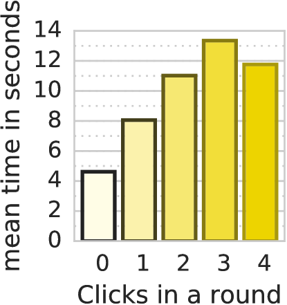
Figure 7: Mean time in seconds per answer type. See section 5.2.2 for discussion.

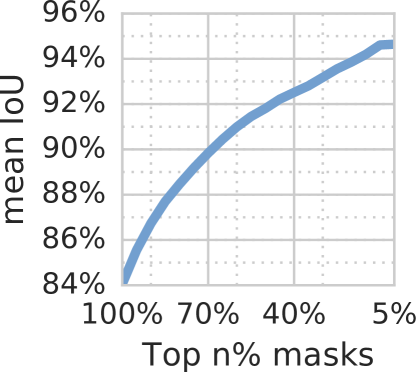
Figure 8: mIoU over $\text{COCO}_{\text{L}}$ for fraction of top ranked samples. $M_{r}$ allows to select high quality subsets of the data.

5.3 Corrective clicks: Time versus quality

Each annotation method presents a different trade-off between speed and quality. Fig. 9 summarizes this for our corrective clicks, COCO polygon annotations, and our free-painted masks. In all cases mIoU is measured w.r.t. the free-painted annotations on the COCO dataset (§4.4 and 5.1).

After three rounds of corrective clicks, we obtain masks with $84\%\ \text{mIoU}$ in an average human annotation time of $34\text{s}$ per instance. In comparison, COCO polygons reach $82\%\ \text{mIoU}$, while taking an estimated $108\text{s}$ per instance (section 5.1). For reference, our free-painted masks take $138\text{s}$ and have a self-agreement of $90\%\ \text{mIoU}$. We observe a similar trend when comparing boundary quality (F-measure at 5 pixels [23, 29]): 75% for our corrective click masks versus 65% for COCO polygons, and 79% for the reference free-painted masks. We thus conclude that our corrective click masks are of higher quality than the COCO polygon annotations, while being $3\times$ faster to make.

Coincidentally, COCO annotations average $33.4$ vertices per instance on the instances considered, and our annotator do an average of $10.7$ clicks per instance over all three rounds of interactive segmentation. Thus the $3\times$ factor also holds in number of clicks. Some examples of our corrective click masks can be seen in figure 6.

Semantic segmentation training

To further validate the utility of the generated corrective click masks, we train from them a DeeplabV3 Xception65 model for semantic segmentation over $\text{COCO}^{train}_{L}$. For comparison, we also train a second model from the original COCO polygon annotations. Since we only annotated large objects ($>80\times 40$ pixels), we ignore small instances during both training and testing. We then evaluate over $\text{COCO}_{\text{L}}^{\text{test}}$ and observe that both models perform comparably ($52\%\ \text{mIoU}$ COCO masks, versus $53\%$ ours).

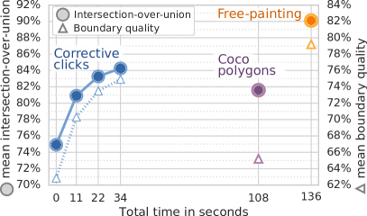
Figure 9: Masks quality versus time for different annotation schemes (section 5.3). Our corrective click masks reach better quality than COCO polygons, while being $3\times$ faster to make.

5.4 Corrective clicks: Masks ranking

Once all our annotations are produced, the $M_{r}$ model can be used to rank them. We train this model on $1\%$ of COCO ground-truth (section 4.2) and then use it to rank all corrective click masks.

Fig. 8 shows mIoU over $\text{COCO}_{\text{L}}$ when selecting the top N% ranked masks (bottom N% plot in supp. material). The slanted shape indicates that $M_{r}$ is effective at sorting the masks. A random ranker would result in a horizontal line. Thanks to $M_{r}$ we can select a higher quality subset of the data (the top 70% masks have $90\%\ \text{mIoU}$), target annotation efforts on the lowest ranking instances (the bottom 30% have $70\%\ \text{mIoU}$), or weight training samples based on their rank. This self-diagnosing capability is a side-effect of using corrective clicks rather than directly drawing the masks.

6 Conclusion

We have shown that interactive segmentation can be a compelling approach for instance segmentation at scale. We have systematically explored the design space of deep interactive segmentation models. Based on the gained insights, we executed a large-scale annotation campaign, producing 2.5M instance masks on OpenImages. These masks are of high quality (84% mIoU, 75% boundary quality). Additionally, we proposed a technique for automatically estimating the quality of individual masks. We plan to publicly release these new annotations hoping they will help further develop the field of instance segmentation.

References

- [1] D. Acuna, H. Ling, A. Kar, and S. Fidler. Efficient interactive annotation of segmentation datasets with polygon-rnn++. In CVPR, 2018.
- [2] J. T. Barron and B. Poole. The fast bilateral solver. In ECCV. Springer, 2016.
- [3] A. Bearman, O. Russakovsky, V. Ferrari, and L. Fei-Fei. What’s the Point: Semantic Segmentation with Point Supervision. In ECCV, 2016.
- [4] Y. Y. Boykov and M.-P. Jolly. Interactive graph cuts for optimal boundary & region segmentation of objects in nd images. In ICCV, 2001.
- [5] L.-C. Chen, G. Papandreou, I. Kokkinos, K. Murphy, and A. L. Yuille. Deeplab: Semantic image segmentation with deep convolutional nets, atrous convolution, and fully connected crfs. PAMI, 2018.
- [6] M. Cordts, M. Omran, S. Ramos, T. Rehfeld, M. Enzweiler, R. Benenson, U. Franke, S. Roth, and B. Schiele. The cityscapes dataset for semantic urban scene understanding. In CVPR, 2016.
- [7] J. Dai, K. He, and J. Sun. Boxsup: Exploiting bounding boxes to supervise convolutional networks for semantic segmentation. In ICCV, 2015.
- [8] M. Everingham, S. M. A. Eslami, L. Van Gool, C. K. I. Williams, J. Winn, and A. Zisserman. The pascal visual object classes challenge: A retrospective. IJCV, 2015.
- [9] B. Hariharan, P. Arbelaez, L. Bourdev, S. Maji, and J. Malik. Semantic contours from inverse detectors. In ICCV, 2011.
- [10] Y. Hu, A. Soltoggio, R. Lock, and S. Carter. A fully convolutional two-stream fusion network for interactive image segmentation. Neural Networks, 2018.
- [11] X. Huang, X. Cheng, Q. Geng, B. Cao, D. Zhou, P. Wang, Y. Lin, and R. Yang. The apolloscape dataset for autonomous driving. arXiv preprint arXiv:1803.06184, 2018.
- [12] A. Khoreva, R. Benenson, J. H. Hosang, M. Hein, and B. Schiele. Simple does it: Weakly supervised instance and semantic segmentation. In CVPR, 2017.
- [13] A. Kirillov. 2018 panoptic segmentation dataset overview.
- [14] A. Kuznetsova, H. Rom, N. Alldrin, J. Uijlings, I. Krasin, J. Pont-Tuset, S. Kamali, S. Popov, M. Malloci, T. Duerig, and V. Ferrari. The open images dataset v4: Unified image classification, object detection, and visual relationship detection at scale. arXiv:1811.00982, 2018.
- [15] H. Le, L. Mai, B. Price, S. Cohen, H. Jin, and F. Liu. Interactive boundary prediction for object selection. In ECCV, pages 18–33, 2018.
- [16] Z. Li, Q. Chen, and V. Koltun. Interactive image segmentation with latent diversity. In CVPR, 2018.
- [17] J. Liew, Y. Wei, W. Xiong, S.-H. Ong, and J. Feng. Regional interactive image segmentation networks. In ICCV, 2017.
- [18] D. Lin, J. Dai, J. Jia, K. He, and J. Sun. Scribblesup: Scribble-supervised convolutional networks for semantic segmentation. In CVPR, 2016.
- [19] T.-Y. Lin, M. Maire, S. Belongie, J. Hays, P. Perona, D. Ramanan, P. Dollár, and C. L. Zitnick. Microsoft coco: Common objects in context. In ECCV, 2014.
- [20] S. Mahadevan, P. Voigtlaender, and B. Leibe. Iteratively trained interactive segmentation. In BMVC, 2018.
- [21] M. Maire, S. X. Yu, and P. Perona. Hierarchical scene annotation. In BMVC, 2013.
- [22] K.-K. Maninis, S. Caelles, J. Pont-Tuset, and L. Van Gool. Deep extreme cut: From extreme points to object segmentation. In CVPR, 2018.
- [23] D. R. Martin, C. C. Fowlkes, and J. Malik. Learning to detect natural image boundaries using local brightness, color, and texture cues. PAMI, 2004.
- [24] G. Neuhold, T. Ollmann, S. Rota Bulò, and P. Kontschieder. The mapillary vistas dataset for semantic understanding of street scenes. In ICCV, 2017.
- [25] D. P. Papadopoulos, A. D. Clarke, F. Keller, and V. Ferrari. Training object class detectors from eye tracking data. In ECCV. Springer, 2014.
- [26] D. P. Papadopoulos, J. R. Uijlings, F. Keller, and V. Ferrari. Extreme clicking for efficient object annotation. In ICCV, 2017.
- [27] D. P. Papadopoulos, J. R. R. Uijlings, F. Keller, and V. Ferrari. Training object class detectors with click supervision. CVPR, 2017.
- [28] M. Pizenberg, A. Carlier, E. Faure, and V. Charvillat. Outlining objects for interactive segmentation on touch devices. In ACM on Multimedia Conference, 2017.
- [29] J. Pont-Tuset and F. Marques. Supervised evaluation of image segmentation and object proposal techniques. PAMI, 2016.
- [30] C. Rother, V. Kolmogorov, and A. Blake. "grabcut": interactive foreground extraction using iterated graph cuts. ACM Trans. Graph., 2004.
- [31] O. Russakovsky, J. Deng, H. Su, J. Krause, S. Satheesh, S. Ma, Z. Huang, A. Karpathy, A. Khosla, M. Bernstein, A. C. Berg, and L. Fei-Fei. ImageNet Large Scale Visual Recognition Challenge. IJCV, 2015.
- [32] C. Sun, A. Shrivastava, S. Singh, and A. Gupta. Revisiting unreasonable effectiveness of data in deep learning era. In ICCV, 2017.
- [33] The Atlantic. ’what are clothes?’ asks most delightful supreme court argument in history.
- [34] G. Wang, M. A. Zuluaga, W. Li, R. Pratt, P. A. Patel, M. Aertsen, T. Doel, A. L. Divid, J. Deprest, S. Ourselin, et al. Deepigeos: a deep interactive geodesic framework for medical image segmentation. PAMI, 2018.
- [35] N. Xu, B. Price, S. Cohen, J. Yang, and T. Huang. Deep grabcut for object selection. In BMVC, 2017.
- [36] N. Xu, B. Price, S. Cohen, J. Yang, and T. S. Huang. Deep interactive object selection. In CVPR, 2016.
- [37] B. Zhou, H. Zhao, X. Puig, S. Fidler, A. Barriuso, and A. Torralba. Scene parsing through ade20k dataset. In CVPR, 2017.
- [38] Y. Zhou, Y. Zhu, Q. Ye, Q. Qiu, and J. Jiao. Weakly supervised instance segmentation using class peak response. In CVPR, 2018.